the Creative Commons Attribution 4.0 License.
the Creative Commons Attribution 4.0 License.
 | 21 Sep 2023
The Teddy tool v1.1: temporal disaggregation of daily climate model data for climate impact analysis
Benjamin Poschlod
Climate models provide the required input data for global or regional climate impact analysis in temporally aggregated form, often in daily resolution to save space on data servers. Today, many impact models work with daily data; however, sub-daily climate information is becoming increasingly important for more and more models from different sectors, such as the agricultural, water, and energy sectors. Therefore, the open-source Teddy tool (temporal disaggregation of daily climate model data) has been developed to disaggregate (temporally downscale) daily climate data to sub-daily hourly values. Here, we describe and validate the temporal disaggregation, which is based on the choice of daily climate analogues. In this study, we apply the Teddy tool to disaggregate bias-corrected climate model data from the Coupled Model Intercomparison Project Phase 6 (CMIP6). We choose to disaggregate temperature, precipitation, humidity, longwave radiation, shortwave radiation, surface pressure, and wind speed. As a reference, globally available bias-corrected hourly reanalysis WFDE5 (WATCH Forcing Data methodology applied to ERA5) data from 1980–2019 are used to take specific local and seasonal features of the empirical diurnal profiles into account. For a given location and day within the climate model data, the Teddy tool screens the reference data set to find the most similar meteorological day based on rank statistics. The diurnal profile of the reference data is then applied on the climate model. The physical dependency between variables is preserved, since the diurnal profile of all variables is taken from the same, most similar meteorological day of the historical reanalysis dataset. Mass and energy are strictly preserved by the Teddy tool to exactly reproduce the daily values from the climate models.
For evaluation, we aggregate the hourly WFDE5 data to daily values and apply the Teddy tool for disaggregation. Thereby, we compare the original hourly data with the data disaggregated by Teddy. We perform a sensitivity analysis of different time window sizes used for finding the most similar meteorological day in the past. In addition, we perform a cross-validation and autocorrelation analysis for 30 globally distributed samples around the world that represent different climate zones. The validation shows that Teddy is able to reproduce historical diurnal courses with high correlations >0.9 for all variables, except for wind speed (>0.75) and precipitation (>0.5). We discuss the limitations of the method regarding the reproduction of precipitation extremes, interday connectivity, and disaggregation of end-of-century projections with strong warming. Depending on the use case, sub-daily data provided by the Teddy tool could make climate impact assessments more robust and reliable.
- Article
(5424 KB) - Full-text XML
-
Supplement
(1978 KB) - BibTeX
- EndNote


Table 1Variables and units of used hourly (h) and daily (d) climate data and the Teddy output. For WFDE5, the specific variable name is provided in parentheses. WFDE5 variables have instantaneous values, while SWdown, LWdown, Rainf, and Snowf have average values over the next hour at each time step.
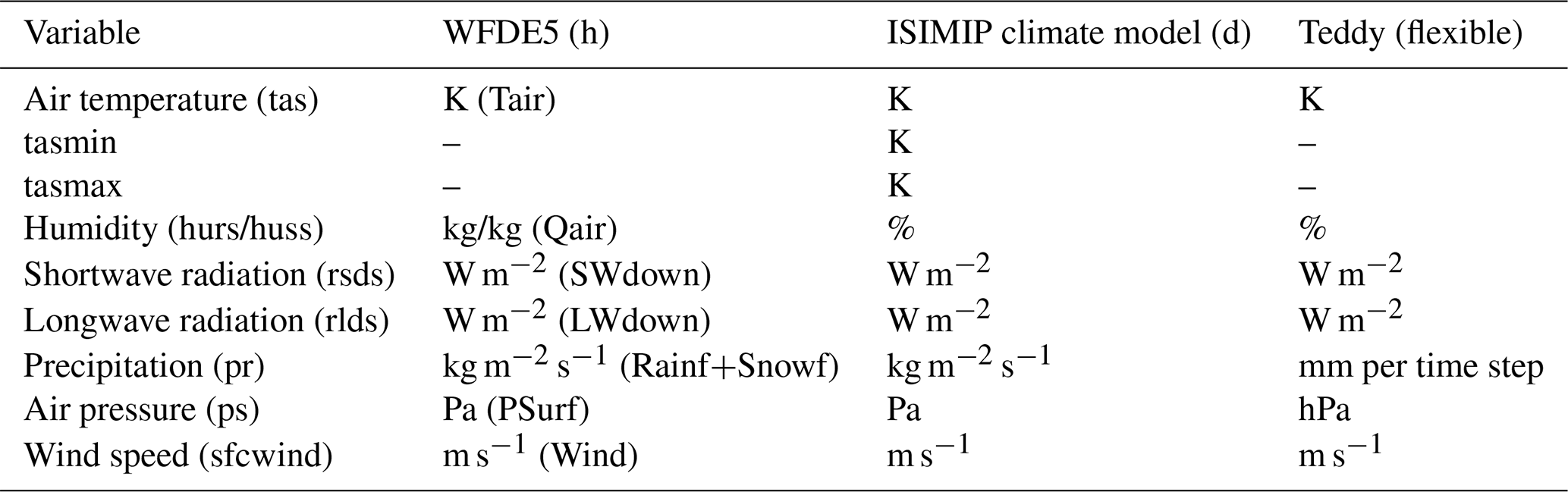
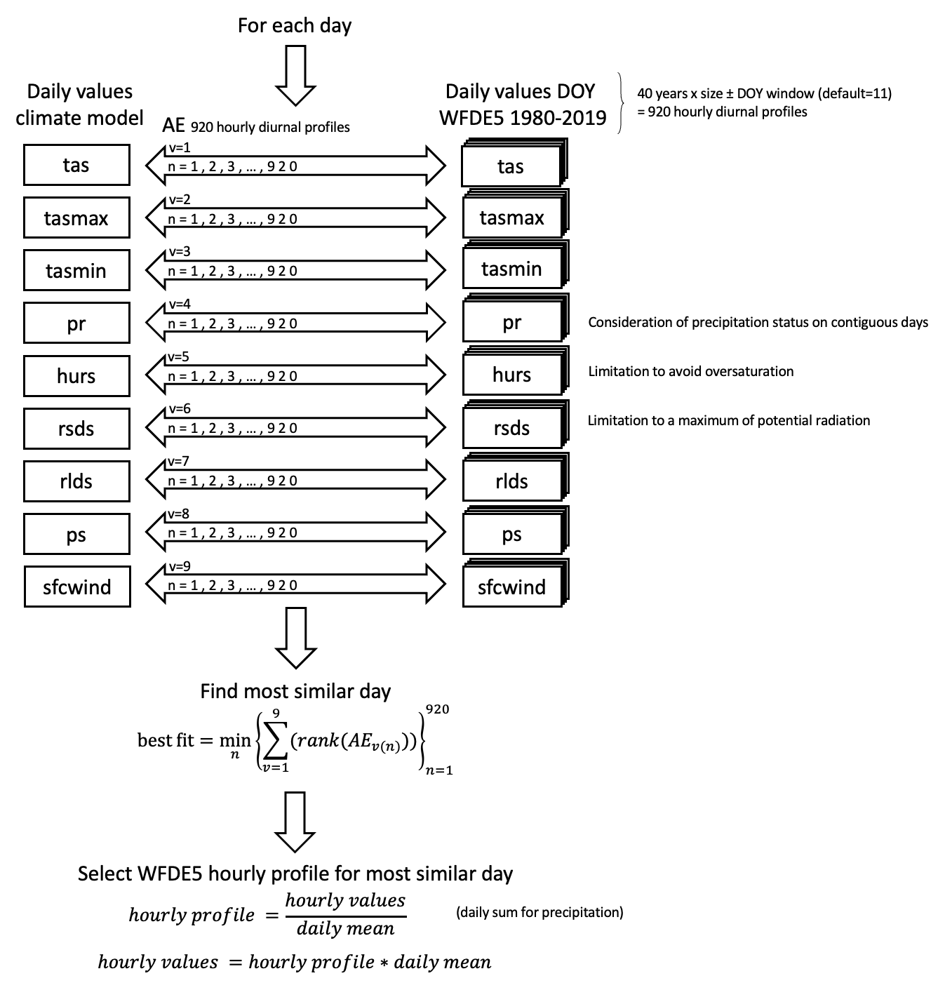
Figure 1Procedure to identify the most similar meteorological day in the population of WFDE5 reference data for the default day of year (DOY) window of ±11 d around the actual DOY. Daily values refer to the daily sum for precipitation and daily mean values for all other variables.
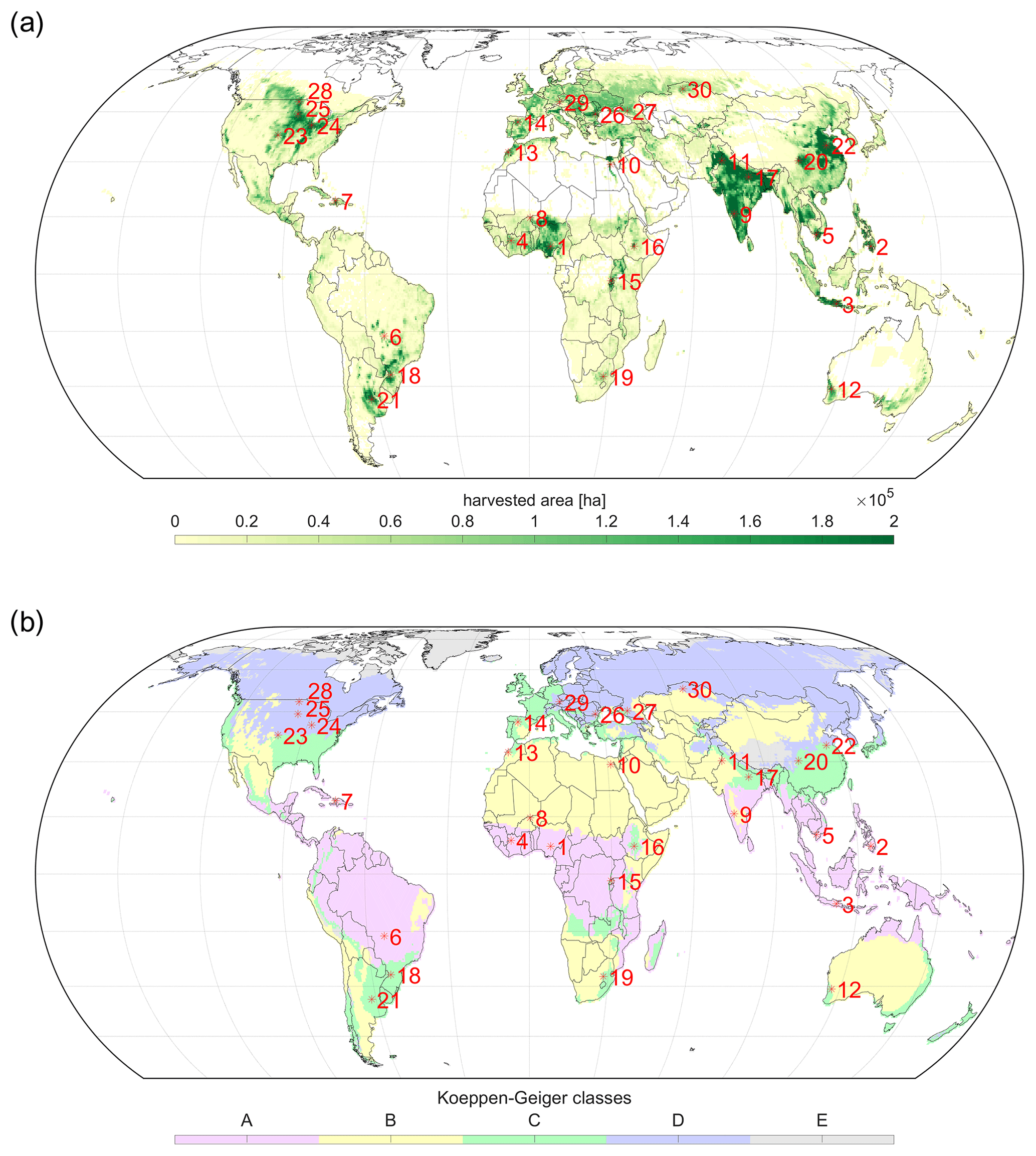
Figure 2Distribution of 30 global samples used for the cross-validation on (a) annual total harvested area of rainfed and irrigated crops in hectare per pixel on a 30 arcmin grid (Portmann et al., 2010) and (b) for Köppen–Geiger climate zones calculated for 1980–2019 WFDE5 temperature and precipitation values (Beck et al., 2018). Samples are ordered by climate zone affiliation and their distance to the Equator.
Sub-daily climate data are becoming increasingly important in climate impact analysis. This type of data, which captures variations in temperature, precipitation, and other weather variables at intervals of less than a day, can provide a more detailed representation of local and regional climate conditions and temporal variations. This information can be crucial for evaluating the impacts of climate change on various sectors, such as agriculture, water resources, energy production, and human health (Golub et al., 2022; Trinanes and Martinez-Urtaza, 2021; Colón-González et al., 2021; Tittensor et al., 2021; Byers et al., 2018; Jägermeyr et al., 2021; Poschlod and Ludwig, 2021; Degife et al., 2021). A better representation of the diurnal course of temperature, extreme precipitation events, and other weather variables is also important for adaptation assessments which depend on behavior or processes with high temporal dynamics, such as the energy demand, labor activity, the heat stress of crops, or flood events (Minoli et al., 2022; Zabel et al., 2021; Reed et al., 2022; Orlov et al., 2021; Franke et al., 2022; Poschlod, 2022). Research has shown that using sub-daily climate data can result in more robust and reliable impact assessments when compared to using daily data (Orlov et al., 2023).
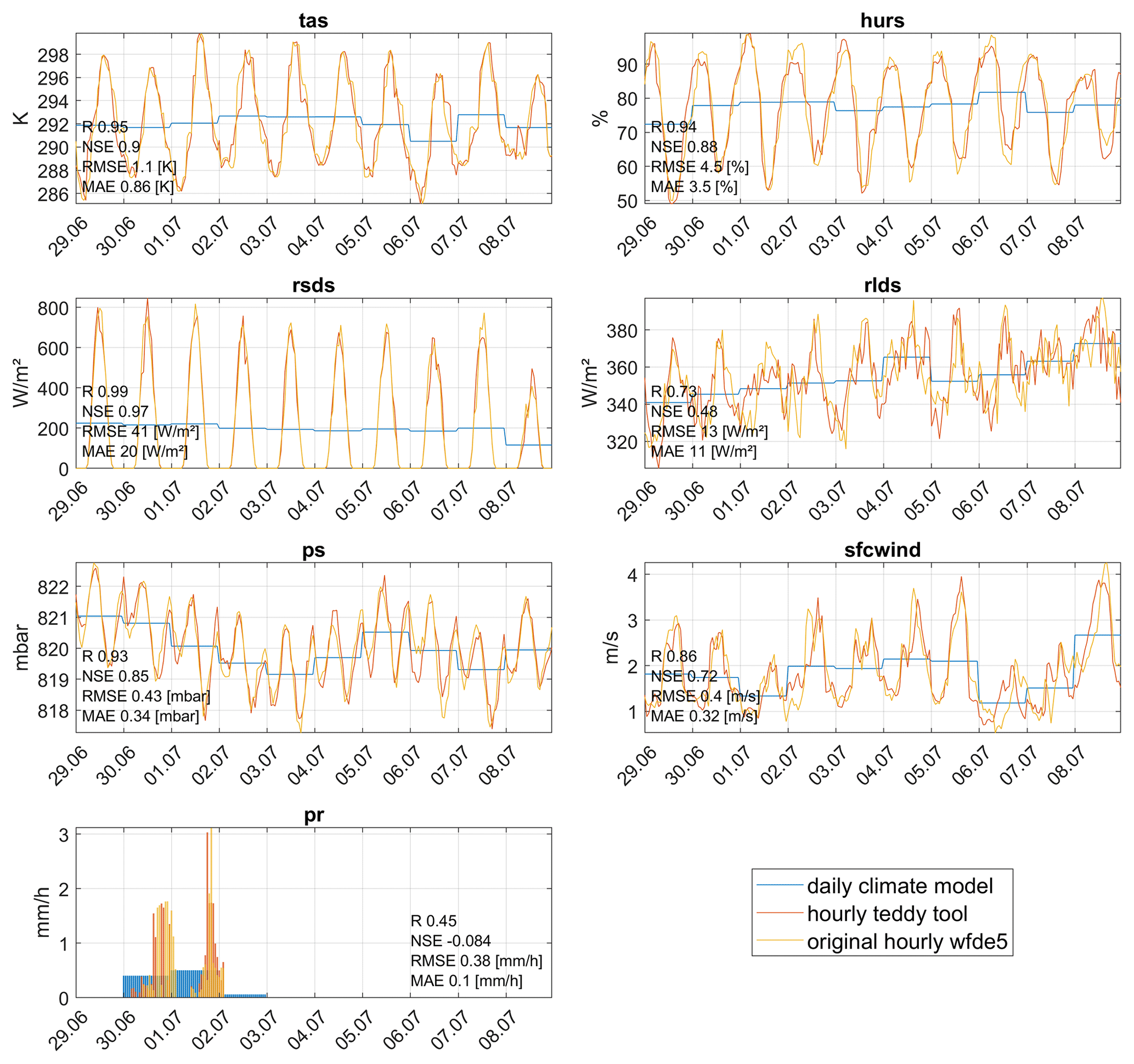
Figure 3Time series for all variables comparing daily climate model data, using disaggregated hourly results of Teddy from the performed cross-validation and the original hourly WFDE5 data, shown for sample location 16 in Ethiopia with a DOY window size of seven for the 10 d period of 29 June–8 July 2010. The Pearson correlation coefficient (R), the Nash–Sutcliffe model efficiency coefficient (NSE), the root mean squared error (RMSE), and the mean absolute error (MAE) are displayed for the shown time period for each variable.
Today, most climate model data are available for download at a daily resolution because of the high storage requirements for sub-daily climate data (Juckes et al., 2020). However, the demand for sub-daily data is increasing, with future developments in data management expected to handle this demand with decreasing costs for storage and computing resources (Lüttgau and Kunkel, 2018). Different methods exist to disaggregate available daily climate data to sub-daily, most often hourly, values. These can be roughly divided into statistical methods, weather generators, and mechanistic approaches, although mixed forms also exist (Förster et al., 2016).
Mechanistic methods use regional climate models to dynamically downscale atmospheric conditions in time and space, usually for a limited area (Vormoor and Skaugen, 2013; Liu et al., 2011; Kunstmann and Stadler, 2005). Weather generators generate synthetic sequences of hourly weather variables by using random number generators that match statistics (Ailliot et al., 2015; Mezghani and Hingray, 2009). Various statistical methods exist for temporal disaggregation of daily climate data, ranging from simple interpolations or deterministic approaches to non-parametric approaches and methods that derive statistical relationships from historical data or look for climate analogues (Bennett et al., 2020; Breinl and Di Baldassarre, 2019; Chen, 2016; Debele et al., 2007; Förster et al., 2016; Görner et al., 2021; Liston and Elder, 2006; Park and Chung, 2020; Verfaillie et al., 2017; Poschlod et al., 2018; Zhao et al., 2021). Each of these methods has its own advantages and limitations, and the choice of method depends on factors such as the specific needs of the impact assessment, the quality of the available data, and the computational resources.
Here, we introduce the Teddy tool (temporal disaggregation of daily climate model data), which uses statistical methods for temporal disaggregation of daily climate model data. Existing statistical approaches are often only valid for a specific location and cannot be applied globally. In addition, available disaggregation tools often focus on only one variable (e.g., Pui et al., 2012) and therefore do not consider physical interdependencies between different variables, such as precipitation, humidity, temperature, and radiation. Teddy has been specifically developed as a globally applicable tool for climate impact studies. For this purpose, Teddy strictly preserves the mass and energy of daily climate model data for each variable throughout the disaggregation procedure. Teddy additionally aims at taking regional and seasonal climate characteristics into account and considers the physical consistency between variables.
Teddy represents an easy-to-use tool that can be applied for climate impact assessments in different sectors that allow a physically consistent temporal disaggregation of daily climate model data. The Teddy tool has been written in MATLAB and is available as open-source code via Zenodo (see the Code availability section at the end of the paper ).
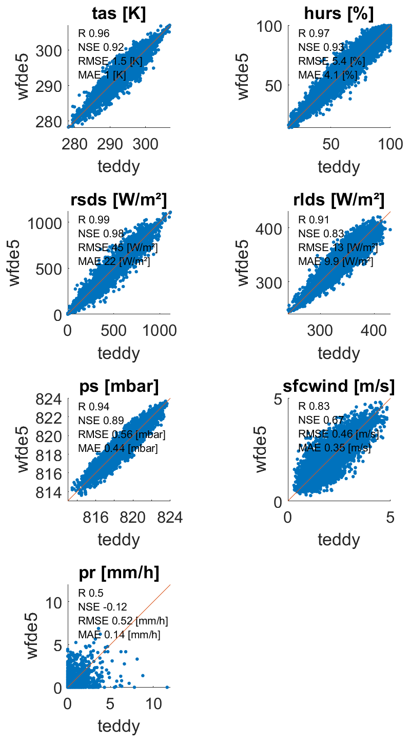
Figure 4Hourly values for the year 2010 between disaggregated values generated by the Teddy tool and the original WFDE5 data used for the cross-validation, exemplarily for sample location 16 in Ethiopia with a DOY window size of seven. The Pearson correlation coefficient (R), the Nash–Sutcliffe model efficiency coefficient (NSE), the root mean squared error (RMSE), and the mean absolute error (MAE) are displayed for each variable.
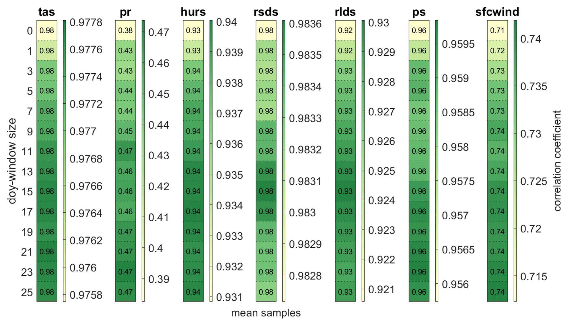
Figure 5Pearson correlation coefficient between disaggregated hourly values generated by the Teddy tool and the original WFDE5 data used for the cross-validation for different DOY window sizes averaged over all 30 samples for the year 2010 for all variables. The scaling of the color bar differs between variables.
In principle, the Teddy tool can be used with any climate input but has specifically been developed to be used with daily climate data for historical time periods and future scenarios from the Inter-Sectoral Impact Model Intercomparison Project (ISIMIP). ISIMIP offers a framework for consistently projecting the impacts of climate change across affected sectors and spatial scales (Warszawski et al., 2014). To guarantee cross-sectoral consistency in ISIMIP, all sectors are provided with the same climate data for historical (1850–2014) and future time periods (2015–2100) for different scenarios (SSP126, SSP370, and SSP585). ISIMIP provides bias-corrected climate model data from the Coupled Model Intercomparison Project Phase 6 (CMIP6; Eyring et al., 2016) and trend-preserving reanalysis climate data (Lange, 2019). Within ISIMIP, some modeling communities from different sectors have expressed their need for sub-daily climate data, including the agricultural and the energy sectors.
Daily bias-corrected climate model data are provided by ISIMIP at 0.5∘ spatial resolution for air temperature (tas), humidity (hurs), shortwave radiation (rsds), longwave radiation (rlds), air pressure (ps), wind speed (sfcwind), and precipitation (pr; Lange, 2019; Lange and Büchner, 2021). For air temperature, the daily maximum (tasmax) and minimum (tasmin) values are additionally provided. ISIMIP provides CMIP6 data for the climate models GFDL-ESM4, IPSL-CM6A-LR, MPI-ESM1-2-HR, MRI-ESM2-0, and UKESM1-0-LL.
Teddy requires hourly climate data as a reference for temporal disaggregation. Therefore, we use the WFDE5 dataset, which has been generated using the WATCH Forcing Data (WFD) methodology applied to ERA5 reanalysis data (Cucchi et al., 2020). The bias-adjusted hourly WFDE5 data are globally available for the time period between 1979 and 2019 at 0.5∘ spatial resolution (Cucchi et al., 2022). It is consistent with the bias-adjustment procedure within ISIMIP (Lange, 2019) and thus provides a consistent hourly reference data for Teddy. Table 1 gives an overview of the available variables and the required datasets at their temporal resolution. The temporal resolution of the Teddy output is adjustable by the user and can be set to 1, 2, 3, 4, 6, 8, or 12 h values.
Teddy uses an empirical approach, which (1) selects the “most similar meteorological day” for the daily climate model data (here ISIMIP CMIP6 data) within the reference climate data (here WFDE5) at the same location. (2) Teddy applies the location-specific diurnal course to each variable of the daily climate model data for a day of interest. In the following, the procedure is explained in detail, where the example case of ISIMIP climate data and WFDE5 reference data is used for further illustration.
In a first precalculation step, in order to minimize computational resources, hourly WFDE5 data are aggregated to daily values and stored as NetCDF files. The daily aggregation uses mean values for all variables and daily sums for precipitation. In addition, rainfall and snowfall fluxes must be summed up for WFDE5. Daily maximum and minimum temperature are calculated from the hourly data. Units of climate inputs are converted to match the Teddy output (see Table 1). For the conversion of specific humidity to relative humidity, the Buck equation is applied (Buck, 1981). After reading the daily climate model data for the selected location (latitude and longitude) that determines a specific grid cell at 0.5∘ resolution, the daily mean values of all ISIMIP variables (see Table 1) are compared to the aggregated daily values of WFDE5 for a specific time step in order to identify the most similar meteorological day. For the comparison, a day-of-year (DOY) window can be selected by the user that allows for a selection of days around the DOY of the actual time step. By default, the DOY window size is set to 11, which means a sequence of ±11 d around the actual DOY. As a result, 23 d are selected from each of the 40 WFDE5 reference years (1980–2019). These 920 d now serve as the statistical population for further calculations (Fig. 1). In a next step, the climate model day of interest and the statistical population of 920 WFDE5 days are classified according to their precipitation state (wet or dry). As climate models tend to produce too many days with low-intensity precipitation called “drizzle bias” (Chen et al., 2021), days with aggregated daily precipitation values below 1 mm per day are considered to be dry days (Sun et al., 2006). Depending on the precipitation state of the previous day, the day of interest, and the following day, there are eight classes, namely dry–dry–dry, dry–dry–wet, wet–dry–dry, wet–dry–wet, dry–wet–dry, dry–wet–wet, wet–wet–dry, and wet–wet–wet. This step is included to better reproduce the interday connectivity of precipitation (Li et al., 2018). Only days with the same precipitation class as the climate model day of interest are selected for the further course. Next, the absolute error (AE) between the daily climate model and aggregated daily WFDE5 data for each variable is calculated for the remaining statistical population and ranked in ascending order. The ranking approach is chosen, since the absolute or relative errors of the different meteorological variables cannot be compared to each other. The ranks are cumulated with equal weight over all variables for each day of the statistical population. In this context, we define the most similar meteorological day as the day with the minimum sum of ranks (Fig. 1). Thus, the most similar meteorological day refers to the statistically derived similarity of all available daily near-surface meteorological variables at a given location and time. The approach works under the assumption that similar daily values would have a similar sub-daily profile (Li et al., 2018; Pui et al., 2012; Sharma and Srikanthan, 2006). Finally, the hourly values are taken from the most similar meteorological day of the WFDE5 reference dataset for each variable and are divided by the WFDE5 daily mean (sum for precipitation) value of the selected day, in order to refer to relative diurnal profiles without absolute variations (Fig. 1). The hourly profile is then applied for each variable to the daily mean (sum for precipitation) value from the climate model. Thus, the daily mean value (sum for precipitation) of the climate model is conserved and reproduced by the disaggregated values.
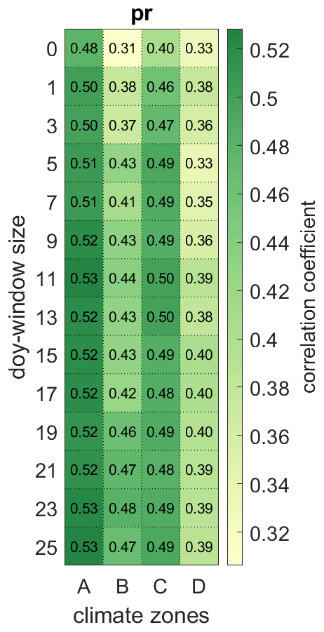
Figure 6Pearson correlation coefficient between disaggregated hourly values generated by the Teddy tool and the original WFDE5 data used for the cross-validation for different DOY window sizes averaged over the samples for each Köppen–Geiger climate zone (A is tropical, B is arid, C is temperate, and D is continental).
For temperature, the resulting hourly temperature is further scaled between the provided minimum and maximum. The scaling is performed in a way that the daily mean value is preserved with an accuracy of four decimals. Relative humidity is limited to 100 %, thus considering the preservation of the daily mean value.
On the one hand, large selected DOY windows increase the statistical population, but on the other hand, they might distort climatic characteristics with a strong seasonal course such as shortwave radiation values for the actual DOY. Therefore, we preprocessed hourly potential (cloud-free) solar radiation for each DOY globally at 0.5∘ spatial resolution. These data are used as an upper bound to limit the resulting hourly values for the corresponding DOY, while the daily mean value is preserved.
In a final step, the hourly values are aggregated to the temporal resolution, as set by the user.
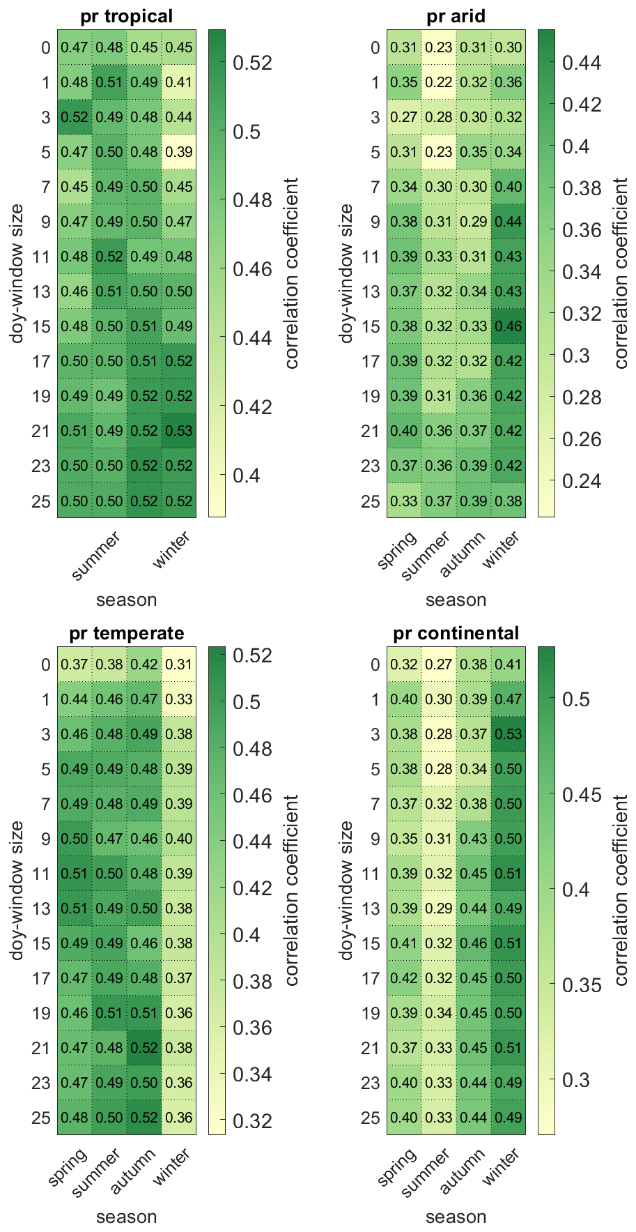
Figure 7Pearson correlation coefficient between disaggregated hourly values generated by the Teddy tool and the original WFDE5 data used for the cross-validation for different DOY window sizes averaged over the samples for the four seasons. The Northern Hemisphere spring is March, April, and May (MAM); summer is June, July, and August (JJA); autumn is September, October, and November (SON); and winter is December, January and February (DJF). The Southern Hemisphere spring is SON, summer is DJF, autumn is MAM, and winter is JJA. The heatmap is averaged over the samples for each Köppen–Geiger climate zone (A is tropical, B is arid, C is temperate, and D is continental).

Figure 8Extended validation statistics for the sensitivity analysis of the DOY window size for the year 2010. The difference in autocorrelation refers to the average over all 30 samples and lag durations between one and 24 h. Wet hours are defined as precipitation intensities above 0.1 mm h−1, and low wind speeds refer to hours with sfcwind <2.5 m s−1.
In rare cases, precipitation cannot be distributed, due to no precipitation being present in the reference data. This can happen in dry deserts, where 40 years of WFDE5 data show no precipitation record within the range of the moving DOY window (Fig. S1 in the Supplement shows a map indicating where this is the case). To handle this exception, several options are implemented. First, the DOY window is automatically expanded to ±50 d around the actual DOY in order to increase the statistical population and thus the probability of including a precipitation event. If still no precipitation event is found in the reference, then a linear regression between the precipitation amount and the precipitation duration is performed for the specific location across the entire available data spectrum. The linear regression determines the usual duration of the selected precipitation event. Subsequently, an hour is randomly selected for the start of the precipitation event. A goal of Teddy was to consider the physical consistency of intervariable relationships. Precipitation generally affects other climate variables (e.g., humidity, radiation, and temperature; Meredith et al., 2021). During the night, physical interdependencies between precipitation and other variables are generally lower because radiation is not affected and less energy is available to affect other variables. This might have an effect for impact models because, as an example, evapotranspiration might be unrealistically high if precipitation occurs at the same time as when there is full solar irradiation during noon. In order to reduce possible inconsistencies with other variables that could lead to implications in impact models, the precipitation is only distributed to hours at nighttime. Alternatively, we implemented the option for the user to write not a number (NaN) values instead.
Drizzle precipitation (values below 1 mm d−1) is also disaggregated to sub-daily values in order to ensure mass and energy conservation. If no historical precipitation event is found for this case, then precipitation noise is again randomly distributed to an hour at nighttime. If no hour without radiation occurs (e.g., high latitudes in northern summer), then the precipitation is distributed to local midnight.
The calculation procedure can be performed either for universal time (UT) or for local solar time (LST). The latter divides the world into equal time zones of 15∘, with the central time zone (±7.5∘) at Greenwich.
In a first step, Teddy is applied for 30 globally distributed samples (Fig. 2) for the year 2010. To be able to validate the results, we perform a cross-validation. Therefore, WFDE5 data for 2010 aggregated to daily values serve as an input for Teddy. The same year is excluded from the statistical population during the cross-validation. As a result, it can be tested to see how well WFDE5 hourly values for the year 2010 are reproduced with the statistical population of the other 39 years. The 30 samples are chosen to represent globally relevant agricultural production regions in different climate zones (Fig. 2). To evaluate the sensitivity of the different DOY window sizes, we run the cross-validation with different DOY window sizes, ranging from 1 to 25, in steps of two, including the option to disable the DOY window (DOY window size =0). In order to additionally validate the performance for extreme events, we perform a second cross-validation for all available 40 years (1980–2019), with DOY window sizes of 11 for sample location 29, which is located in southern Germany.
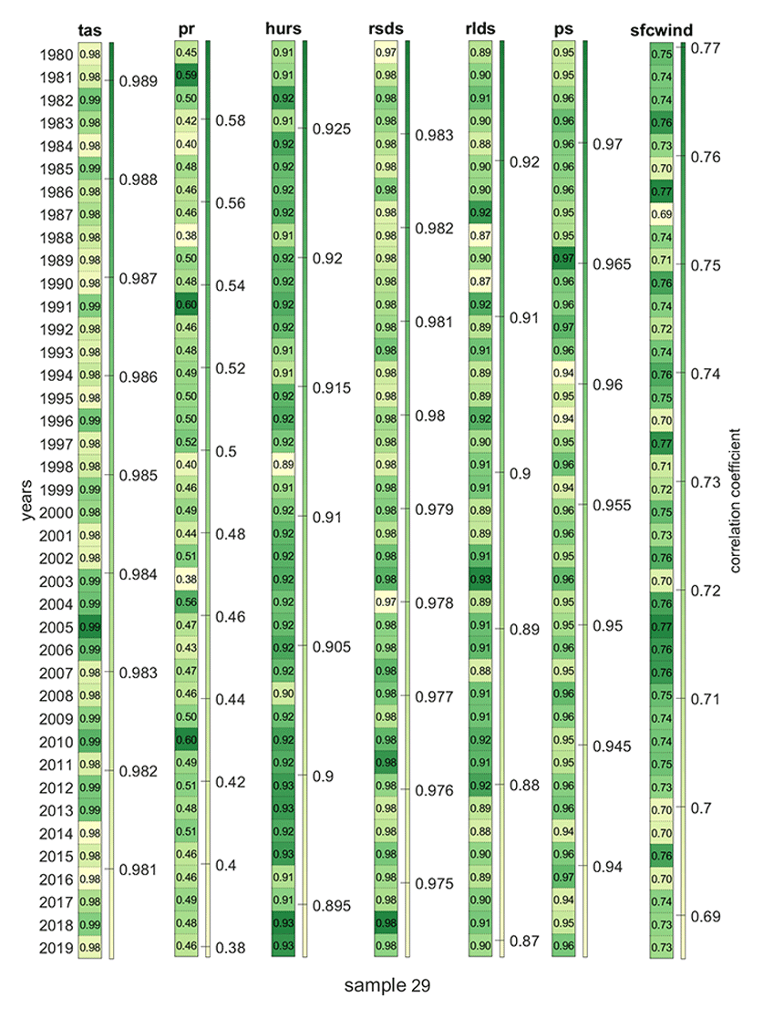
Figure 9Pearson correlation coefficient between disaggregated hourly values generated by the Teddy tool and the original WFDE5 data used for the cross-validation for each year from 1980 to 2019 for sample location 29 and a DOY window size of 11 d. The scaling of the color bar differs between variables.
4.1 Validation
As an example, for sample location 16 in Ethiopia, Fig. 3 shows the results of the temporal disaggregation series for the cross-validation for a 10 d time series in 2010 in comparison with the daily climate input and the original hourly WFDE5 data. The hourly courses show high correlations for the randomly selected time series for all variables, except for precipitation (Fig. 3 and scatterplots in Fig. 4 for the entire year; Figs. S2 and S3 alternatively show sample location 22 in China).
4.2 Sensitivity analysis DOY window size
The sensitivity analysis averaged over all 30 samples shows that the Pearson correlation coefficient of hourly values for the year 2010 shows high correlations for all variables (r>0.9), except wind speed (r>0.7) and precipitation (r>0.4), which are generally more difficult to disaggregate (Fig. 5; in the Supplement, Fig. S4 additionally shows the Nash–Sutcliffe model efficiency coefficient). The selected DOY window size has an effect on the quality of the results. While no DOY window (size =0) results in the lowest correlation coefficient across all variables, the DOY window size does significantly affect the correlation for precipitation and wind speed (Fig. 5).
For precipitation, the impact of the DOY window size on the correlation varies between regions. Larger DOY windows are mainly beneficial for precipitation in arid regions, while showing lower increases in correlation in regions with pronounced seasons (Fig. 6). The results also show that the correlation for precipitation is generally larger in tropical regions than in continental regions.
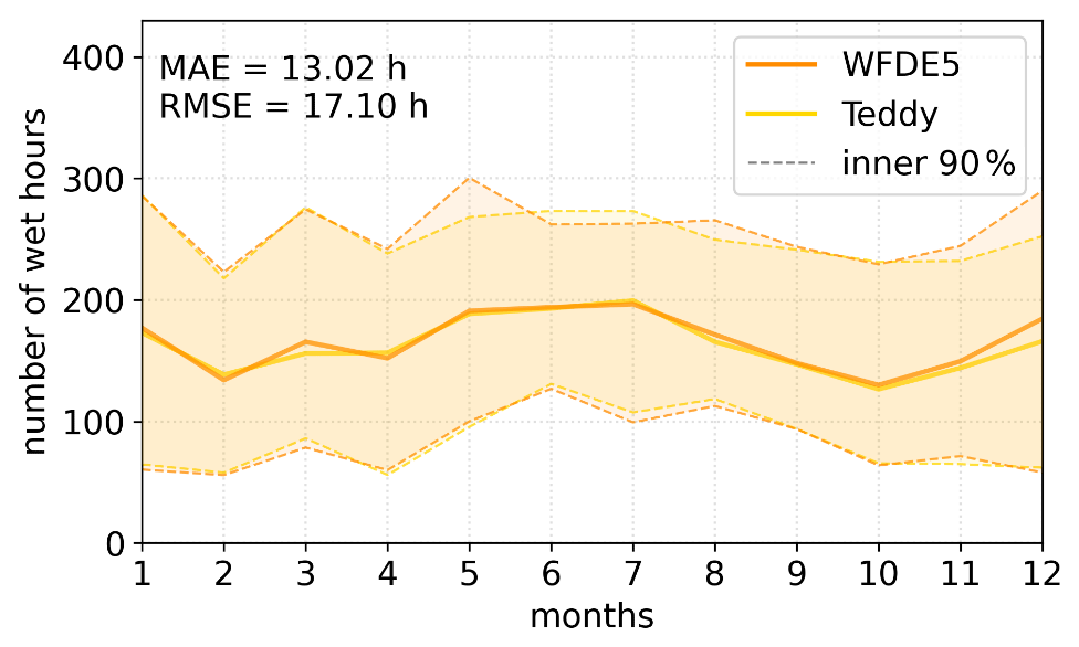
Figure 10Number of wet hours per month for sample location 29 in Germany. Solid lines show the median over 40 years, whereas the dashed lines denote the inner 90 % of the 40-year period. MAE and RMSE are calculated separately for every year and averaged over 40 years.
While hourly precipitation can be best reproduced for winter seasons in continental and arid regions, winter seasons show the lowest correlation for temperate regions. Tropical regions only show relatively low variations over the year, and these are independent of the selected DOY window size (Fig. 7). Especially in arid regions, the length of the DOY window size affects the results differently in different seasons. Here, larger DOY windows decrease the correlation during the rainy season (winter and spring), while correlation is increased during the dry season (summer and autumn).
Furthermore, we evaluate the sensitivity of the DOY window size to the reproduction of temporal autocorrelation (Fig. 8). Therefore, the autocorrelation over lag times between 1 and 24 h is calculated for precipitation and wind speed. Autocorrelation refers to the similarity of a time series to a lag-duration-shifted version of the same time series. This allows sub-daily patterns and interhour connectivity to be statistically captured and validated in time series of precipitation and wind speed. In addition, we also check the reproduction of wet hours (precipitation above 0.1 mm h−1) in 2010 and the number of hours with low wind speeds (sfcwind <2.5 m s−1) referring to the typical cut-in wind speed of wind turbines.
Here, we find that short DOY window sizes below 5 d are not beneficial to all statistics. The autocorrelation of precipitation (wind speed) is reproduced more accurately with window sizes of 9 d or longer. The number of wet hours is better recreated with window sizes above 15 d. For hours with low wind speed, a minor improvement is found above 9 d.
4.3 Multiyear evaluation
The previous validation has assessed the disaggregation performance for all sample locations for the year 2010 and different DOY window sizes. For the analysis of the whole time period of 1980–2019, we evaluate each year of the 40-year time series for sample location 29 and a window size of 11 d. Figures 9 and S5 show the correlation coefficient and mean absolute error, respectively, for each year to assess the interannual variability in the disaggregation performance. For tas, hurs, rsds, rlds, and ps, the performance shows only very minor differences, whereas sfcwind and pr show a higher degree of interannual fluctuations.
4.4 Evaluation of precipitation: wet proportions and intensities
For a further evaluation of precipitation characteristics, we additionally assess the disaggregated time series over the whole period 1980–2019 for sample location 29. In order to evaluate the reproduction of wet : dry proportions, the monthly cycle of wet hours is provided (Fig. 10). Wet hours above 0.1 mm h−1 are recreated by the Teddy tool, with minor differences for the median over 40 years (Fig. 10). The error measures are calculated for every year separately, amounting to a mean absolute error of 13.02 h equaling 7.8 %.
For the evaluation of the range of precipitation intensities, Fig. 11 shows intensities above 1 mm h−1 plotted against its percentage of exceedance for sub-daily durations. We find that the disaggregated precipitation intensities match the original data, except for extreme precipitation.
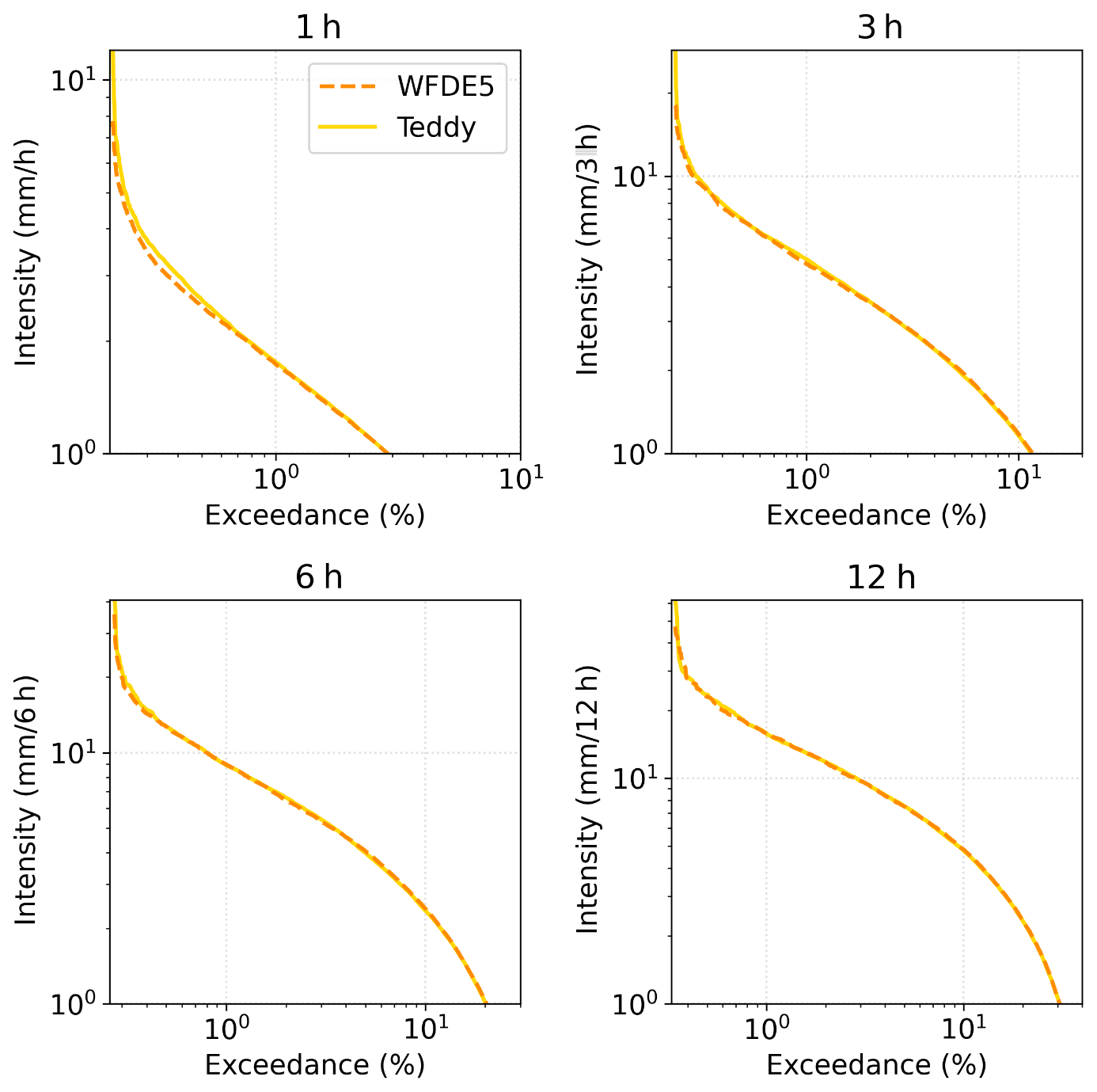
Figure 11Exceedance probability of precipitation intensities for sub-daily durations for sample location 29 in Germany.
4.5 Evaluation of precipitation extremes
As the ISIMIP database is used for future impact modeling and historical attribution science (Mengel et al., 2021), the extremes are of major interest to the community. The ability of global climate models to simulate sub-daily extremes is limited and depends on the variable of interest and the spatiotemporal conditions of the extreme and the respective model setup (Wehner et al., 2021; Kumar et al., 2015; Wang and Clow, 2020). However, in this validation, we evaluate how the Teddy tool is able to preserve the statistics of sub-daily extreme values. Therefore, we select precipitation as variable of interest. Figure 12 shows the reproduction of sub-daily precipitation extremes for 1980–2019 for sample location 29 in southern Germany, where Teddy is run with a DOY window size of 11 d. The 40 annual maxima are extracted from the original and the disaggregated data. Additionally, the generalized extreme value (GEV) distribution is fitted to these empirical data. GEV parameters are estimated via maximum likelihood estimation (MLE; Coles, 2001), where the goodness of fit is assessed with the Anderson–Darling test at 95 % significance level (Stephens, 1986). Thereby, 95 % confidence intervals are generated when applying a bootstrap procedure with 1000 iterations to account for extreme value statistical uncertainties. We find that the Teddy tool leads to an overestimation of annual maximum precipitation. For the hourly duration, the differences are large, with the confidence intervals of the GEV hardly overlapping. For longer durations, Teddy values approach the original data, with noticeable differences only for the rare events with return periods longer than 5 years.
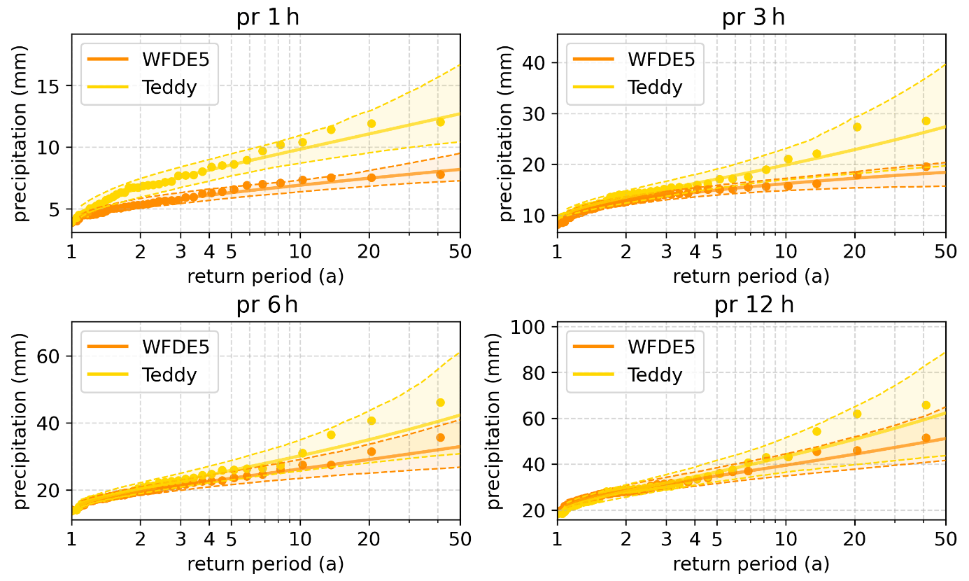
Figure 12Extreme value statistical evaluation of sub-daily precipitation for sample location 29 in Germany. The annual maxima of the WFDE5 and Teddy are shown as dots. Additionally, GEV fits (lines) with 95 % confidence intervals (transparent areas and dashed lines) account for uncertainties. The Teddy tool is run with a DOY window size of 11 d.
The Teddy tool allows for temporal disaggregation of daily climate model data. The disaggregation is based on the location and time-specific empirical relationships between variables. The approach is well suited to all tested variables and results in very high correlations (>0.9), except for precipitation (>0.5) and wind speed (>0.75). We attribute the worse performance for precipitation and wind speed to the high intraday variability for these variables (Watters et al., 2021). Other variables are governed by a stronger diurnal cycle (Dai and Trenberth, 2004), which is easier to disaggregate, based on empirical diurnal profiles.
Compared to other approaches, the advantage of the Teddy tool is that no input data other than the daily climate model data are required. The Teddy tool is relatively simple to apply, considers specific local and seasonal features of the diurnal course of different climate variables, and preserves the physical consistency of intervariable relationships. Mass and energy are conserved, and mean daily values of the climate model are reproduced any time.
The spatial and temporal resolution of the results is determined by the provided temporal and spatial resolution of the chosen reference data (WFDE5 is used here). Longer available reanalysis time periods extend the statistical population for identifying the most similar weather conditions in the past and thus could improve the results. Generally, other reference data could also be used that provide a higher temporal or spatial resolution for a specific region.
The DOY window to find the most similar historical weather situations can be chosen in different sizes. For most of the variables, we found small effects of time window adjustments, except for precipitation and wind speed. The evaluation of different DOY window sizes reveals that a DOY window size of 11 can generally be recommended across all variables. Larger DOY windows should be avoided mainly in arid regions, while shorter DOY windows generally lead to poorer representations of autocorrelation and extreme events.
One limitation of the Teddy tool is the representation of extreme events, mainly for precipitation, which is generally the most difficult variable for temporal disaggregation. We found that hourly precipitation extremes are overestimated. For heavy daily precipitation events, Teddy distributes the 24 h sums either correctly, too evenly, or across too few hours. When distributing across too few hours, extreme hourly intensities evolve, which may have never occurred or may even be physically implausible. For temporal disaggregation of extreme precipitation, we recommend dynamical downscaling via high-resolution climate models (Poschlod, 2021; Poschlod et al., 2021; Zabel et al., 2012; Zabel and Mauser, 2013).
Another limitation of the approach is the reproduction of the interday connectivity within the disaggregated time series. When two diurnal profiles are chosen for the disaggregation of adjacent days which show dissimilar courses in the time steps at the change in the day, abrupt value jumps might occur in the disaggregation. This can be seen in Fig. 3 for rlds from 4 to 5 July. To illustrate this issue, a disaggregation time series from another location is provided in Fig. S2. This limitation also applies for the method of fragments applied on precipitation (Li et al., 2018). Similar to Li et al. (2018), we also consider the precipitation state of the previous and following day to improve interday connectivity. Without this additional consideration, overnight precipitation events would often be “cut off” in the disaggregation. For the remaining abrupt jumps in the disaggregated time series, we refrain from post-processing with subsequent smoothing, as we want to preserve both mass and energy and the empirical diurnal profiles.
For the disaggregation of future climate projections using the Teddy tool, we have the following remarks. As the Teddy tool derives the relationships between sub-daily and daily values empirically based on reanalysis data, future diurnal profiles, which are outside the historical range of diurnal profiles, might possibly be not fully reproduced. However, this limitation is common for statistical approaches which are calibrated on historical data (Papalexiou et al., 2018). Nevertheless, due to energy and mass conservation, climate trends in the daily climate signal are fully preserved. Hence, applying Teddy for temporal disaggregation under climate change holds under the assumption that we select the most similar meteorological day of the historical data and that this diurnal profile is representative of future climatic conditions. However, this assumption might apply to a different degree for different variables. We expect non-stationarity for the diurnal profiles due to changing weather patterns, shifts in rainfall-generating processes, and shifts in the seasonality, mainly for precipitation and wind. The daily course of other variables, such as solar radiation and temperature might generally be less affected by a warmer climate. Furthermore, global climate models at coarse resolutions generally do not represent all processes to fully reproduce intraday variability. Teddy applies the diurnal profiles and intraday variability from the WFDE5 data, which are bias-adjusted ERA5 reanalysis data that implicitly consider finer-scale effects compared to coarse-resolution global climate models (Cucchi et al., 2020). Thus, the disaggregation process in Teddy is consistent with the bias adjustment in ISIMIP3.
Another limitation of the methodology could occur in the case of strong climate change signals. In case of high warming in end-of-century projections, the number of sampled historical days might decrease if the same historical day is sampled repeatedly. This could lead to reductions in diversity of the diurnal profile. Hence, Teddy allows the monitoring of the number of unique analogue days per year. An additional analysis for SSP370 using the GFDL-ESM4 climate model shows that the number of unique analogue climate days is declining, as expected, but still the diversity of chosen days is above 300 unique days at the end of the century for a chosen moving window size of ±11 d (Fig. S6). A smaller size of the moving window prevents a situation in which the same analogue day is chosen over a longer time period. This will increase the diversity of the diurnal profiles at the expense of similarity. Even if diurnal profiles are derived from the same analogue day repeatedly, the disaggregated diurnal courses, e.g., for temperature, will show variations (different offset and different amplitude) due to the conservation of daily mean energy and mass. From a broader perspective, it is also not clear whether the uncertainties resulting from this limitation are larger than the uncertainties within the climate model projections until the end of the century. Furthermore, in the long term, the basic population for finding analogue climates will continuously increase, since WFDE5 data, which are based on ERA5, are continuously updated. We note that Teddy could be also employed to disaggregate future daily climate projections based on hourly future climate projections as reference.
Further possible developments could include improvements in the reproduction of the interday connectivity. Despite the consideration of precipitation classes, abrupt value jumps over day changes are still possible. A future introduction of temperature classes and surface pressure classes in addition to the precipitation classes could help to reduce this effect. Depending on the location of interest, also including climate modes or weather patterns for the choice of the most similar meteorological day could positively affect the performance. Furthermore, depending on the application, it could be reasonable not to screen for the most similar meteorological day but for the most similar succession of multiple days. This would consequently improve the interday connectivity as fewer different profiles are selected.
Other optional future developments could include the separation of direct and diffuse radiation, which is also a required information for some impact models and which is currently not provided by ISIMIP. However, we would make further development, with more options being dependent on the community's adoption of the current executable tool.
The source code of the Teddy tool (v1.1) and a parallelized version of the Teddy tool (v1.1p), including a precompiled executable file for Windows, preprocessed data, results of the cross-validation, and exemplary results for SSP585 (2015–2100) and the UKESM1-0-L climate model for 30 samples are provided via Zenodo (https://doi.org/10.5281/zenodo.8124111, Zabel and Poschlod, 2023).
The supplement related to this article is available online at: https://doi.org/10.5194/gmd-16-5383-2023-supplement.
FZ: conceptualization, software, methodology, validation, formal analysis, resources, data curation, writing the original draft, and visualization. BP: methodology, validation, formal analysis, writing the original draft, and visualization.
The contact author has declared that none of the authors has any competing interests.
Publisher’s note: Copernicus Publications remains neutral with regard to jurisdictional claims in published maps and institutional affiliations.
We acknowledge the methodological discussion with Stefan Lange from the Potsdam Institute of Climate Impact Research (PIK).
This open-access publication was funded by Ludwig-Maximilians-Universität München.
This paper was edited by Di Tian and reviewed by three anonymous referees.
Ailliot, P., Allard, D., Monbet, V., and Naveau, P.: Stochastic weather generators: an overview of weather type models, Journal de la Société Française de Statistique, 156, 101–113, 2015.
Beck, H. E., Zimmermann, N. E., McVicar, T. R., Vergopolan, N., Berg, A., and Wood, E. F.: Present and future Köppen-Geiger climate classification maps at 1-km resolution, Sci. Data, 5, 180214, https://doi.org/10.1038/sdata.2018.214, 2018.
Bennett, A., Hamman, J., and Nijssen, B.: MetSim: A python package for estimation and disaggregation of meteorological data, J. Open Source Softw., 5, 2042, https://doi.org/10.21105/joss.02042, 2020.
Breinl, K. and Di Baldassarre, G.: Space-time disaggregation of precipitation and temperature across different climates and spatial scales, Journal of Hydrology: Regional Studies, 21, 126–146, https://doi.org/10.1016/j.ejrh.2018.12.002, 2019.
Buck, A. L.: New Equations for Computing Vapor Pressure and Enhancement Factor, J. Appl. Meteorol. Clim., 20, 1527–1532, https://doi.org/10.1175/1520-0450(1981)020<1527:Nefcvp>2.0.Co;2, 1981.
Byers, E., Gidden, M., Leclère, D., Balkovic, J., Burek, P., Ebi, K., Greve, P., Grey, D., Havlik, P., Hillers, A., Johnson, N., Kahil, T., Krey, V., Langan, S., Nakicenovic, N., Novak, R., Obersteiner, M., Pachauri, S., Palazzo, A., Parkinson, S., Rao, N. D., Rogelj, J., Satoh, Y., Wada, Y., Willaarts, B., and Riahi, K.: Global exposure and vulnerability to multi-sector development and climate change hotspots, Environ. Res. Lett., 13, 055012, https://doi.org/10.1088/1748-9326/aabf45, 2018.
Chen, C. J.: Temporal disaggregation of seasonal forecasting for streamflow simulation, World Environmental and Water Resources Congress, 2016, West Palm Beach, Florida, 22–26 May 2016, https://doi.org/10.1061/9780784479858.008, 63–72, 2016.
Chen, D., Dai, A., and Hall, A.: The Convective-To-Total Precipitation Ratio and the “Drizzling” Bias in Climate Models, J. Geophys. Res.-Atmos., 126, e2020JD034198, https://doi.org/10.1029/2020JD034198, 2021.
Coles, S.: An Introduction to Statistical Modeling of Extreme Values, Springer, London, UK, https://doi.org/10.1007/978-1-4471-3675-0, 2001.
Colón-González, F. J., Sewe, M. O., Tompkins, A. M., Sjödin, H., Casallas, A., Rocklöv, J., Caminade, C., and Lowe, R.: Projecting the risk of mosquito-borne diseases in a warmer and more populated world: a multi-model, multi-scenario intercomparison modelling study, Lancet Planetary Health, 5, e404-e414, https://doi.org/10.1016/S2542-5196(21)00132-7, 2021.
Cucchi, M., Weedon, G. P., Amici, A., Bellouin, N., Lange, S., Müller Schmied, H., Hersbach, H., and Buontempo, C.: WFDE5: bias-adjusted ERA5 reanalysis data for impact studies, Earth Syst. Sci. Data, 12, 2097–2120, https://doi.org/10.5194/essd-12-2097-2020, 2020.
Cucchi, M., Weedon, G. P., Amici, A., Bellouin, N., Lange, S., Müller Schmied, H., Hersbach, H., Cagnazzo, C., and Buontempo, C.: Near surface meteorological variables from 1979 to 2019 derived from bias-corrected reanalysis, version 2.1, Copernicus Climate Change Service (C3S) Climate Data Store (CDS) [data set], https://doi.org/10.24381/cds.20d54e34, 2022.
Dai, A. and Trenberth, K. E.: The Diurnal Cycle and Its Depiction in the Community Climate System Model, J. Climate, 17, 930–951, https://doi.org/10.1175/1520-0442(2004)017<0930:TDCAID>2.0.CO;2, 2004.
Debele, B., Srinivasan, R., and Yves Parlange, J.: Accuracy evaluation of weather data generation and disaggregation methods at finer timescales, Adv. Water Resour., 30, 1286–1300, https://doi.org/10.1016/j.advwatres.2006.11.009, 2007.
Degife, A. W., Zabel, F., and Mauser, W.: Climate change impacts on potential maize yields in Gambella region, Ethiopia, Reg. Environ. Change, 21, 12, https://doi.org/10.1007/s10113-021-01773-3, 2021.
Eyring, V., Bony, S., Meehl, G. A., Senior, C. A., Stevens, B., Stouffer, R. J., and Taylor, K. E.: Overview of the Coupled Model Intercomparison Project Phase 6 (CMIP6) experimental design and organization, Geosci. Model Dev., 9, 1937–1958, https://doi.org/10.5194/gmd-9-1937-2016, 2016.
Förster, K., Hanzer, F., Winter, B., Marke, T., and Strasser, U.: An open-source MEteoroLOgical observation time series DISaggregation Tool (MELODIST v0.1.1), Geosci. Model Dev., 9, 2315–2333, https://doi.org/10.5194/gmd-9-2315-2016, 2016.
Franke, J. A., Müller, C., Minoli, S., Elliott, J., Folberth, C., Gardner, C., Hank, T., Izaurralde, R. C., Jägermeyr, J., Jones, C. D., Liu, W., Olin, S., Pugh, T. A. M., Ruane, A. C., Stephens, H., Zabel, F., and Moyer, E. J.: Agricultural breadbaskets shift poleward given adaptive farmer behavior under climate change, Glob. Change Biol., 28, 167–181, https://doi.org/10.1111/gcb.15868, 2022.
Golub, M., Thiery, W., Marcé, R., Pierson, D., Vanderkelen, I., Mercado-Bettin, D., Woolway, R. I., Grant, L., Jennings, E., Kraemer, B. M., Schewe, J., Zhao, F., Frieler, K., Mengel, M., Bogomolov, V. Y., Bouffard, D., Côté, M., Couture, R.-M., Debolskiy, A. V., Droppers, B., Gal, G., Guo, M., Janssen, A. B. G., Kirillin, G., Ladwig, R., Magee, M., Moore, T., Perroud, M., Piccolroaz, S., Raaman Vinnaa, L., Schmid, M., Shatwell, T., Stepanenko, V. M., Tan, Z., Woodward, B., Yao, H., Adrian, R., Allan, M., Anneville, O., Arvola, L., Atkins, K., Boegman, L., Carey, C., Christianson, K., de Eyto, E., DeGasperi, C., Grechushnikova, M., Hejzlar, J., Joehnk, K., Jones, I. D., Laas, A., Mackay, E. B., Mammarella, I., Markensten, H., McBride, C., Özkundakci, D., Potes, M., Rinke, K., Robertson, D., Rusak, J. A., Salgado, R., van der Linden, L., Verburg, P., Wain, D., Ward, N. K., Wollrab, S., and Zdorovennova, G.: A framework for ensemble modelling of climate change impacts on lakes worldwide: the ISIMIP Lake Sector, Geosci. Model Dev., 15, 4597–4623, https://doi.org/10.5194/gmd-15-4597-2022, 2022.
Görner, C., Franke, J., Kronenberg, R., Hellmuth, O., and Bernhofer, C.: Multivariate non-parametric Euclidean distance model for hourly disaggregation of daily climate data, Theor. Appl. Climatol., 143, 241–265, https://doi.org/10.1007/s00704-020-03426-7, 2021.
Jägermeyr, J., Müller, C., Ruane, A. C., Elliott, J., Balkovic, J., Castillo, O., Faye, B., Foster, I., Folberth, C., Franke, J. A., Fuchs, K., Guarin, J. R., Heinke, J., Hoogenboom, G., Iizumi, T., Jain, A. K., Kelly, D., Khabarov, N., Lange, S., Lin, T.-S., Liu, W., Mialyk, O., Minoli, S., Moyer, E. J., Okada, M., Phillips, M., Porter, C., Rabin, S. S., Scheer, C., Schneider, J. M., Schyns, J. F., Skalsky, R., Smerald, A., Stella, T., Stephens, H., Webber, H., Zabel, F., and Rosenzweig, C.: Climate impacts on global agriculture emerge earlier in new generation of climate and crop models, Nature Food, 2, 873–885, https://doi.org/10.1038/s43016-021-00400-y, 2021.
Juckes, M., Taylor, K. E., Durack, P. J., Lawrence, B., Mizielinski, M. S., Pamment, A., Peterschmitt, J.-Y., Rixen, M., and Sénési, S.: The CMIP6 Data Request (DREQ, version 01.00.31), Geosci. Model Dev., 13, 201–224, https://doi.org/10.5194/gmd-13-201-2020, 2020.
Kumar, D., Mishra, V., and Ganguly, A. R.: Evaluating wind extremes in CMIP5 climate models, Clim. Dynam., 45, 441–453, https://doi.org/10.1007/s00382-014-2306-2, 2015.
Kunstmann, H. and Stadler, C.: High resolution distributed atmospheric-hydrological modelling for Alpine catchments, J. Hydrol., 314, 105–124, https://doi.org/10.1016/j.jhydrol.2005.03.033, 2005.
Lange, S.: Trend-preserving bias adjustment and statistical downscaling with ISIMIP3BASD (v1.0), Geosci. Model Dev., 12, 3055–3070, https://doi.org/10.5194/gmd-12-3055-2019, 2019.
Lange, S. and Büchner, M.: ISIMIP3b bias-adjusted atmospheric climate input data (v1.1), ISIMIP Repository [data set], https://doi.org/10.48364/ISIMIP.842396.1, 2021.
Li, X., Meshgi, A., Wang, X., Zhang, J., Tay, S. H. X., Pijcke, G., Manocha, N., Ong, M., Nguyen, M. T., and Babovic, V.: Three resampling approaches based on method of fragments for daily-to-subdaily precipitation disaggregation, Int. J. Climatol., 38, e1119–e1138, https://doi.org/10.1002/joc.5438, 2018.
Liston, G. E. and Elder, K.: A Meteorological Distribution System for High-Resolution Terrestrial Modeling (MicroMet), J. Hydrometeorol., 7, 217–234, https://doi.org/10.1175/jhm486.1, 2006.
Liu, C., Ikeda, K., Thompson, G., Rasmussen, R., and Dudhia, J.: High-Resolution Simulations of Wintertime Precipitation in the Colorado Headwaters Region: Sensitivity to Physics Parameterizations, Mon. Weather Rev., 139, 3533–3553, https://doi.org/10.1175/MWR-D-11-00009.1, 2011.
Lüttgau, J. and Kunkel, J.: Cost and Performance Modeling for Earth System Data Management and Beyond, in: High Performance Computing, edited by: Yokota, R., Weiland, M., Shalf, J., and Alam, S., ISC High Performance 2018, Lecture Notes in Computer Science, Springer, Cham, 11203, https://doi.org/10.1007/978-3-030-02465-9_2, 2018.
Mengel, M., Treu, S., Lange, S., and Frieler, K.: ATTRICI v1.1 – counterfactual climate for impact attribution, Geosci. Model Dev., 14, 5269–5284, https://doi.org/10.5194/gmd-14-5269-2021, 2021.
Meredith, E., Ulbrich, U., Rust, H. W., and Truhetz, H.: Present and future diurnal hourly precipitation in 0.11∘ EURO-CORDEX models and at convection-permitting resolution, Environ. Res. Commun., 3, 055002, https://doi.org/10.1088/2515-7620/abf15e, 2021.
Mezghani, A. and Hingray, B.: A combined downscaling-disaggregation weather generator for stochastic generation of multisite hourly weather variables over complex terrain: Development and multi-scale validation for the Upper Rhone River basin, J. Hydrol., 377, 245–260, https://doi.org/10.1016/j.jhydrol.2009.08.033, 2009.
Minoli, S., Jägermeyr, J., Asseng, S., Urfels, A., and Müller, C.: Global crop yields can be lifted by timely adaptation of growing periods to climate change, Nat. Commun., 13, 7079, https://doi.org/10.1038/s41467-022-34411-5, 2022.
Orlov, A., Daloz, A. S., Sillmann, J., Thiery, W., Douzal, C., Lejeune, Q., and Schleussner, C.: Global Economic Responses to Heat Stress Impacts on Worker Productivity in Crop Production, Economics of Disasters and Climate Change, 5, 367–390, https://doi.org/10.1007/s41885-021-00091-6, 2021.
Orlov, A., et al.: Human heat stress could offset economic benefits of the CO2 fertilisation effect in crop production, Nat. Commun., under review, 2023.
Papalexiou, S. M., Markonis, Y., Lombardo, F., AghaKouchak, A., and Foufoula-Georgiou, E.: Precise Temporal Disaggregation Preserving Marginals and Correlations (DiPMaC) for Stationary and Nonstationary Processes, Water Resour. Res., 54, 7435–7458, https://doi.org/10.1029/2018WR022726, 2018.
Park, H. and Chung, G.: A Nonparametric Stochastic Approach for Disaggregation of Daily to Hourly Rainfall Using 3-Day Rainfall Patterns, Water, 12, 2306, https://doi.org/10.3390/w12082306, 2020.
Portmann, F. T., Siebert, S., and Döll, P.: MIRCA2000–Global monthly irrigated and rainfed crop areas around the year 2000: A new high-resolution data set for agricultural and hydrological modeling, Global Biogeochem. Cy., 24, GB1011, https://doi.org/10.1029/2008GB003435, 2010.
Poschlod, B.: Using high-resolution regional climate models to estimate return levels of daily extreme precipitation over Bavaria, Nat. Hazards Earth Syst. Sci., 21, 3573–3598, https://doi.org/10.5194/nhess-21-3573-2021, 2021.
Poschlod, B.: Attributing heavy rainfall event in Berchtesgadener Land to recent climate change – Further rainfall intensification projected for the future, Weather and Climate Extremes, 38, 100492, https://doi.org/10.1016/j.wace.2022.100492, 2022.
Poschlod, B. and Ludwig, R.: Internal variability and temperature scaling of future sub-daily rainfall return levels over Europe, Environ. Res. Lett., 16, 064097, https://doi.org/10.1088/1748-9326/ac0849, 2021.
Poschlod, B., Hodnebrog, Ø., Wood, R. R., Alterskjær, K., Ludwig, R., Myhre, G., and Sillmann, J.: Comparison and Evaluation of Statistical Rainfall Disaggregation and High-Resolution Dynamical Downscaling over Complex Terrain, J. Hydrometeorol., 19, 1973–1982, https://doi.org/10.1175/jhm-d-18-0132.1, 2018.
Poschlod, B., Ludwig, R., and Sillmann, J.: Ten-year return levels of sub-daily extreme precipitation over Europe, Earth Syst. Sci. Data, 13, 983–1003, https://doi.org/10.5194/essd-13-983-2021, 2021.
Pui, A., Sharma, A., Mehrotra, R., Sivakumar, B., and Jeremiah, E.: A comparison of alternatives for daily to sub-daily rainfall disaggregation, J. Hydrol., 470, 138–157, https://doi.org/10.1016/j.jhydrol.2012.08.041, 2012.
Reed, C., Anderson, W., Kruczkiewicz, A., Nakamura, J., Gallo, D., Seager, R., and McDermid, S. S.: The impact of flooding on food security across Africa, P. Natl. Acad. Sci. USA, 119, e2119399119, https://doi.org/10.1073/pnas.2119399119, 2022.
Sharma, A. and Srikanthan, S.: Continuous Rainfall Simulation: A Nonparametric Alternative, in: 30th Hydrology & Water Resources Symposium: Past, Present & Future, 4–7 December 2006, Launceston, Tasmania, p. 86, 2006.
Stephens, A. M.: Tests based on EDF statistics, in: Goodness-of-fit techniques, edited by: D'Agostino, R. B. and Stephens, M. A., Marcel Dekker, New York, 1986.
Sun, Y., Solomon, S., Dai, A., and Portmann, R. W.: How Often Does It Rain?, J. Climate, 19, 916–934, https://doi.org/10.1175/jcli3672.1, 2006.
Tittensor, D. P., Novaglio, C., Harrison, C. S., Heneghan, R. F., Barrier, N., Bianchi, D., Bopp, L., Bryndum-Buchholz, A., Britten, G. L., Büchner, M., Cheung, W. W. L., Christensen, V., Coll, M., Dunne, J. P., Eddy, T. D., Everett, J. D., Fernandes-Salvador, J. A., Fulton, E. A., Galbraith, E. D., Gascuel, D., Guiet, J., John, J. G., Link, J. S., Lotze, H. K., Maury, O., Ortega-Cisneros, K., Palacios-Abrantes, J., Petrik, C. M., du Pontavice, H., Rault, J., Richardson, A. J., Shannon, L., Shin, Y.-J., Steenbeek, J., Stock, C. A., and Blanchard, J. L.: Next-generation ensemble projections reveal higher climate risks for marine ecosystems, Nat. Clim. Change, 11, 973–981, https://doi.org/10.1038/s41558-021-01173-9, 2021.
Trinanes, J. and Martinez-Urtaza, J.: Future scenarios of risk of Vibrio infections in a warming planet: a global mapping study, Lancet Planetary Health, 5, e426–e435, https://doi.org/10.1016/S2542-5196(21)00169-8, 2021.
Verfaillie, D., Déqué, M., Morin, S., and Lafaysse, M.: The method ADAMONT v1.0 for statistical adjustment of climate projections applicable to energy balance land surface models, Geosci. Model Dev., 10, 4257–4283, https://doi.org/10.5194/gmd-10-4257-2017, 2017.
Vormoor, K. and Skaugen, T.: Temporal Disaggregation of Daily Temperature and Precipitation Grid Data for Norway, J. Hydrometeorol., 14, 989–999, https://doi.org/10.1175/jhm-d-12-0139.1, 2013.
Wang, K. and Clow, G. D.: The Diurnal Temperature Range in CMIP6 Models: Climatology, Variability, and Evolution, J. Climate, 33, 8261–8279, https://doi.org/10.1175/jcli-d-19-0897.1, 2020.
Warszawski, L., Frieler, K., Huber, V., Piontek, F., Serdeczny, O., and Schewe, J.: The Inter-Sectoral Impact Model Intercomparison Project (ISI–MIP): Project framework, P. Natl. Acad. Sci. USA, 111, 3228–3232, https://doi.org/10.1073/pnas.1312330110, 2014.
Watters, D., Battaglia, A., and Allan, R.: The Diurnal Cycle of Precipitation according to Multiple Decades of Global Satellite Observations, Three CMIP6 Models, and the ECMWF Reanalysis, J. Climate, 34, 5063–5080, https://doi.org/10.1175/JCLI-D-20-0966.1, 2021.
Wehner, M., Lee, J., Risser, M., Ullrich, P., Gleckler, P., and Collins, W. D.: Evaluation of extreme sub-daily precipitation in high-resolution global climate model simulations, Philos. T. Roy. Soc. A, 379, 20190545, https://doi.org/10.1098/rsta.2019.0545, 2021.
Zabel, F. and Mauser, W.: 2-way coupling the hydrological land surface model PROMET with the regional climate model MM5, Hydrol. Earth Syst. Sci., 17, 1705–1714, https://doi.org/10.5194/hess-17-1705-2013, 2013.
Zabel, F. and Poschlod, B.: Teddy tool v1.1: Temporal Disaggregation of Daily Climate Model Data (1.1), Zenodo [code], https://doi.org/10.5281/zenodo.8124111, 2023.
Zabel, F., Mauser, W., Marke, T., Pfeiffer, A., Zängl, G., and Wastl, C.: Inter-comparison of two land-surface models applied at different scales and their feedbacks while coupled with a regional climate model, Hydrol. Earth Syst. Sci., 16, 1017–1031, https://doi.org/10.5194/hess-16-1017-2012, 2012.
Zabel, F., Müller, C., Elliott, J., Minoli, S., Jägermeyr, J., Schneider, J. M., Franke, J. A., Moyer, E., Dury, M., Francois, L., Folberth, C., Liu, W., Pugh, T. A. M., Olin, S., Rabin, S. S., Mauser, W., Hank, T., Ruane, A. C., and Asseng, S.: Large potential for crop production adaptation depends on available future varieties, Glob. Change Biol., 27, 3870–3882 https://doi.org/10.1111/gcb.15649, 2021.
Zhao, W., Kinouchi, T., and Nguyen, H. Q.: A framework for projecting future intensity-duration-frequency (IDF) curves based on CORDEX Southeast Asia multi-model simulations: An application for two cities in Southern Vietnam, J. Hydrol., 598, 126461, https://doi.org/10.1016/j.jhydrol.2021.126461, 2021.