A comparison of Eulerian and Lagrangian methods for vertical particle transport in the water column

A common task in oceanography is to model the vertical movement of particles such as microplastics, nanoparticles, mineral particles, gas bubbles, oil droplets, fish eggs, plankton, or algae. In some cases, the distribution of the vertical rise or settling velocities of the particles in question can span a wide range, covering several orders of magnitude, often due to a broad particle size distribution or differences in density. This requires numerical methods that are able to adequately resolve a wide and possibly multi-modal velocity distribution.

Lagrangian particle methods are commonly used for these applications. A strength of such methods is that each particle can have its own rise or settling speed, which makes it easy to achieve a good representation of a continuous distribution of speeds. An alternative approach is to use Eulerian methods, where the partial differential equations describing the transport problem are solved directly with numerical methods. In Eulerian methods, different rise or settling speeds must be represented as discrete classes, and in practice, only a limited number of classes can be included.

Here, we consider three different examples of applications for a water column model: positively buoyant fish eggs, a mixture of positively and negatively buoyant microplastics, and positively buoyant oil droplets being entrained by waves. For each of the three cases, we formulate a model for the vertical transport based on the advection–diffusion equation with suitable boundary conditions and, in one case, a reaction term. We give a detailed description of an Eulerian and a Lagrangian implementation of these models, and we demonstrate that they give equivalent results for selected example cases. We also pay special attention to the convergence of the model results with an increasing number of classes in the Eulerian scheme and with the number of particles in the Lagrangian scheme. For the Lagrangian scheme, we see the $\mathrm{1}/\sqrt{N_p}$ convergence, as expected for a Monte Carlo method, while for the Eulerian implementation, we see a second-order ($\mathrm{1}/N_k^{\mathrm{2}}$) convergence with the number of classes.

1 Introduction

Studying the vertical transport of positively, negatively, or neutrally buoyant particles is a common task in oceanography. Examples include both anthropogenic and naturally occurring particles, such as microplastics, mineral particles, nanoparticles, aggregates, gas bubbles, oil droplets, fish eggs, or even particles with active swimming behaviour such as zooplankton. These particles may show a range of different behaviours, including rising, sinking, and interacting with the ocean surface and seafloor in different ways.

Vertical transport modelling may be applied at different scales. In a simple one-dimensional water column model, the goal may be to investigate the timescale of settling or surfacing for a specific type of particle. However, accurate modelling of vertical transport is also key to predicting horizontal transport at large scales, due for example to the vertical variability of horizontal ocean currents (Röhrs et al., 2018; Wichmann et al., 2019). Hence, a good description of vertical behaviour is an essential part of any three-dimensional model.

Commonly used transport models may be divided into two classes: Eulerian and Lagrangian. Eulerian methods consist of solving the advection–diffusion–reaction equation directly with numerical methods for partial differential equations. Ocean circulation models, such as ROMS (Shchepetkin and McWilliams, 2005) or NEMO (Madec et al., 2022), are typical examples of Eulerian models. Related are computational fluid dynamics (CFD) models, which can be used, for example, to model waves and turbulence on smaller scales (Cui et al., 2020). Eulerian models are also used to compute the transport of suspended particles in water, for example natural sediments (Warner et al., 2008), nanoparticles in rivers (Saharia et al., 2019), or microplastics in the oceans (Mountford and Morales Maqueda, 2019).

A challenge of the Eulerian approach, when it comes to particles with a distribution of rise or settling speeds, is that one must use discrete speed classes and solve the advection–diffusion equation for each class, forming a large system of equations to solve simultaneously. Hence, it is of interest to know how many classes are needed to achieve the desired accuracy.

Lagrangian particle methods are quite a popular choice for modelling particle transport in the ocean (van Sebille et al., 2018). In these methods, numerical particles, also called Lagrangian elements, are used to represent physical particles. The numerical particles will move with the current, may exhibit some form of random displacement to model turbulent diffusion, and may have a vertical rise or settling speed (or even active swimming behaviour). Lagrangian particle methods have been applied to transport modelling of a wide range of particle types and processes, including plastics (Delandmeter and Van Sebille, 2019; de La Fuente et al., 2021; Fischer et al., 2022), the residence time of water masses (Dugstad et al., 2019), the transport and sedimentation of mineral particles in the ocean (Dissanayake et al., 2014; Nepstad et al., 2020), the surfacing and entrainment of oil (Cui et al., 2018; Nordam et al., 2019b), the transport of dissolved gases (Dissanayake et al., 2012; Wimalaratne et al., 2015), produced water (Nepstad et al., 2022), harmful algae (Rowe et al., 2016), dinocysts and foraminifera (Van Sebille et al., 2015; Nooteboom et al., 2019), fish eggs (Sundby, 1983; Röhrs et al., 2014), and even fish (Scutt Phillips et al., 2018). Stochastic particle transport methods are also used in many other fields of science, including the study of cosmic rays and high-energy particles from the sun (Strauss and Effenberger, 2017), the deposition of inhaled nanoparticles in the airways (Longest and Xi, 2007), and transport modelling of airborne virus transmission (Abuhegazy et al., 2020).

One of the advantages of a Lagrangian approach to particle transport modelling is the ability to represent a wide range of properties or behaviours. By letting each numerical particle with its own properties move independently of the others, one can model physical particle distributions where the sizes, and hence the terminal velocities, can vary by several orders of magnitude.

In practice, Eulerian and Lagrangian models may offer complementary benefits, and they are often used together. This can be as simple as forcing a Lagrangian model with pre-calculated fields from an Eulerian model (offline Lagrangian modelling; see e.g. Young et al., 2015), or it can involve running a Lagrangian model as part of an Eulerian model (online Lagrangian modelling). In the latter case, it is also possible for the Lagrangian particles to impact the Eulerian model. As examples, Marsh et al. (2015) and Matsumura and Ohshima (2015) model, respectively, icebergs and frazil ice as Lagrangian particles with feedback to the Eulerian model.

The purpose of this paper is to compare and discuss Eulerian and Lagrangian methods, with a focus on the numerical implementation of the models including different boundary conditions and a reaction term. We demonstrate that the two implementations give the same results, and we also address questions of efficiency and convergence. The methods are illustrated using three different one-dimensional cases as a basis for the discussion: fish eggs, microplastics, and oil droplets. The cases have been chosen because they represent simplified (but realistic) cases, and they highlight how particles can interact with the boundaries in different ways.

We consider the water column without background flow and investigate the vertical transport of different types of particles. In Sect. 2, we describe the advection–diffusion equation, which is a partial differential equation (PDE) that will form the basis of our transport problems. Additionally, we present a stochastic differential equation (SDE), which yields a Lagrangian particle method that is equivalent to the advection–diffusion equation. In Sect. 3, we briefly outline how we implement an Eulerian model based on numerically solving the advection–diffusion equation with PDE methods, and similarly, we show how we implement a Lagrangian model based on numerically solving the equivalent SDE for a large ensemble of particles.

In Sect. 4, we apply our Eulerian and Lagrangian water column models to three different cases: fish eggs, microplastics, and oil droplets. All three cases are modelled both with the Eulerian approach and the Lagrangian approach. In each case, the particles considered have a distribution of rising and/or sinking speeds. Additionally, the cases serve to highlight the effects of different boundary conditions and a source term. In Sect. 5, we discuss and summarise our comparison of the Eulerian and Lagrangian approaches. Finally, in Sect. 6, we present some concluding remarks.

Some additional details are given in the Appendices: Appendix A contains detailed descriptions of our Eulerian and Lagrangian model implementations, Appendix B has details on how we obtained a distribution of terminal velocities for microplastics, and Appendix C shows additional numerical convergence results.

2 Components of the advection–diffusion reaction model

2.1 The advection–diffusion equation

As our starting point, we assume that the movement of a collection of particles with different rise or settling velocities in the water column may be described by the advection–diffusion equation (see e.g. Hundsdorfer and Verwer, 2003). If C_k(z,t) is the concentration of particles with (constant) vertical rise or settling speed w_k, then we have

$$\begin{array}{}\text{(1)}& {\displaystyle \frac{\partial C_k}{\partial t}}={\displaystyle \frac{\partial }{\partial z}}\left(K\left(z\right){\displaystyle \frac{\partial C_k}{\partial z}}\right)-{\displaystyle \frac{\partial }{\partial z}}\left(w_k{C}_k\right),\end{array}$$

where K(z) is the diffusivity. To represent a distribution of particle sizes, densities, and/or shapes and thus a distribution of rise speeds, one must, in principle, solve a set of advection–diffusion equations, with one equation for each particle speed w_k.

2.2 Equation of motion of Lagrangian particles

A mathematically equivalent formulation of the advection–diffusion problem is to consider an ensemble of numerical particles, whose positions develop in time according to the stochastic differential equation (SDE):

$$\begin{array}{}\text{(2)}& \mathrm{d}z=(w+K^{\prime }(z\left)\right)\mathrm{d}t+\sqrt{\mathrm{2}K\left(z\right)}\mathrm{d}{W}_t.\end{array}$$

Here, W_t is a standard Wiener process (Kloeden and Platen, 1992, p. 40); K(z) is again the diffusivity as a function of depth; K^′(z) is its derivative with respect to z; and w is the terminal velocity due to buoyancy, which is constant for a given particle.

The connection between Eqs. (1) and (2) is that the probability distribution for the position of particles moving according to Eq. (2) will develop according to Eq. (1). A solution, z(t), to Eq. (2) is called an Itô diffusion, and Eq. (1) is the corresponding Fokker–Planck equation (Kloeden and Platen, 1992, p. 37; see also Appendix A of Nordam et al., 2019b). Each numerical particle position, determined from the SDE, represents a sample from the probability distribution of particle positions, which develops according to the PDE. Solving Eq. (2) for a sufficient number of particles allows us to approximate the probability distribution, which is proportional to the concentration in the Eulerian scheme.

2.3 Velocity distribution

In many practical applications, one will have a size distribution of particles obtained from measurements, a model, or other estimates. For the model we consider here, however, the relevant property is not the size itself but the terminal rise or settling speed of the particle, which is a function of size (and other particle parameters such as shape and density, as well as the viscosity of the ambient fluid). Note that we assume here that a particle will immediately attain its terminal velocity and that particle motion can be described as the combination of a constant terminal velocity and a series of random displacements. This is a commonly used approximation, which holds well if the timescale needed to reach terminal velocity is short compared to other relevant timescales. As an example, consider a particle with some initial speed v₀, moving in water under the influence of Stokes' drag (see Appendix B). Then we have that the initial speed will decay exponentially, as given by

$$\begin{array}{}\text{(3)}& v\left(t\right)=v_{\mathrm{0}}{e}^{-t/\mathit{\tau }},\end{array}$$

where $\mathit{\tau }=\frac{m}{\mathrm{6}\mathit{\pi }\mathit{\mu }r}$, with μ being the dynamic viscosity of water, r being the radius of the particle, and m being the mass of the particle. For typical values for small particles in water, the timescale τ is less than a second (e.g. μ=0.0017 Pa s, r=1 mm, and $m=\mathrm{4}\times {\mathrm{10}}^{-\mathrm{6}}$ kg give τ=0.14 s).

In the example cases we consider in Sect. 4, we will assume that we have access to the distribution of terminal velocities, either by directly specifying a functional form of the velocity distribution or by numerical means through mapping the particle size distribution and other properties to velocities.

2.4 Boundary conditions

Depending on the application, different boundary conditions may be used to control the fluxes across the domain boundaries in a water column model. We will deal separately with the diffusive flux,

$$\begin{array}{}\text{(4)}& j_{\mathrm{D}}\left(z\right)=-K\left(z\right){\left.{\displaystyle \frac{\partial C_k}{\partial z}}\right|}_z,\end{array}$$

and the advective flux

$$\begin{array}{}\text{(5)}& j_{\mathrm{A}}\left(z\right)=w_k{C}_k\left(z\right).\end{array}$$

For the boundary conditions for the diffusive flux, we first observe that diffusion in our model represents the mixing that occurs due to the combination of random turbulent fluctuations and molecular diffusion (Thorpe, 2005, p. 20). Being caused by the motion of the water, the diffusive flux should not allow suspended particles to leave the water column. Hence, we wish to enforce zero diffusive flux, j_D=0, across the boundaries at both the surface and the seafloor. This applies in all the cases we consider in this paper.

Next, we consider the advective flux. In our model, the advection velocity w_k represents the terminal rising or sinking velocity of a particle due to buoyancy. Depending on the application, this velocity may or may not allow particles to leave the water column. As an example, consider positively buoyant fish eggs. When fish eggs rise to the surface, they can of course rise no further. However, they remain submerged, having a hydrophilic surface and a density only slightly less than that of the surrounding seawater. Hence, we have chosen to model fish eggs with a zero-flux boundary condition at the surface. With the surface being at z=0 (and z being negative downwards), the total flux j_tot(z) at the surface is then given by

$$\begin{array}{}\text{(6)}& j_{\mathrm{tot}}\left(\mathrm{0}\right)=j_{\mathrm{A}}\left(\mathrm{0}\right)+j_{\mathrm{D}}\left(\mathrm{0}\right)=\mathrm{0}.\end{array}$$

As another example, consider positively buoyant oil droplets. When oil droplets rise to the surface, they go from being individual droplets surrounded by water to forming small patches of floating oil at the surface or possibly to merging with a larger surface slick. When this happens, the oil droplets are no longer subject to random motion due to turbulent diffusion, and the oil will remain at the surface until some high-energy event like a breaking wave causes the surface slick to break up and form droplets.

To express the mechanism of oil droplets surfacing and leaving the water column, we have two options: we can use a loss term, which removes oil droplets close to the surface at some rate (Tkalich and Chan, 2002), or we can use a partially absorbing boundary condition. Here, we have chosen to allow the advective flux to carry oil droplets across the boundary at the air–sea interface while still enforcing zero diffusive flux across the surface:

$$\begin{array}{}\text{(7)}& j_{\mathrm{tot}}\left(\mathrm{0}\right)=j_{\mathrm{A}}\left(\mathrm{0}\right)+j_{\mathrm{D}}\left(\mathrm{0}\right)=w_k{C}_k\left(\mathrm{0}\right).\end{array}$$

The reasons we describe the surfacing of oil droplets through the boundary condition instead of a loss term are that it is straightforward to express the boundary condition in both the Eulerian and the Lagrangian implementations and that we do not have to define what it means to be close to the surface for the loss term. The idea behind allowing an advective flux while forcing the diffusive flux to be zero is that buoyancy is the mechanism that leads to surfacing. Additionally, if the diffusive flux out of the system is nonzero, then increased diffusivity would lead to faster surfacing, which is contrary to observations. For an additional discussion of this point, see Nordam et al. (2019a).

We note that similar reasoning to the above also applies to the boundary at the seafloor. For example, the settling out of negatively buoyant particles (microplastics, sediments, etc.) can be modelled as an advective flux leaving the model domain through the bottom boundary (i.e. settling on the seafloor or being incorporated into sediments). Note also that, here, advective flux means the flux due to the rise or settling speed of the particle and not that due to vertical currents.

2.5 Reaction terms

An additional reaction term $S_k(z,C_{\mathrm{1}},C_{\mathrm{2}},\mathrm{\dots },C_{N_k})$ may be included in Eq. (1), in which case it becomes the advection–diffusion–reaction equation. It can describe the addition of mass (a source); the removal of mass (a sink); or the transformation of mass between classes, for example from C₁ to C₂, which means that, in general, the reaction term for class k can depend on the concentration of all classes. In an Eulerian implementation, a reaction term can simply add or remove mass in different locations. In a Lagrangian stochastic particle implementation, Eq. (2) only describes the transport of numerical particles, and reaction terms have to be implemented as a separate step, with details depending on the nature of the reaction.

In this study, we will only consider reaction terms that add mass. The reaction term S has units equal to the time derivative of concentration, and it enters our Eulerian scheme in a straightforward manner as a rate of change in the average concentration inside a cell.

For the Lagrangian implementation, adding particles is done in a stochastic manner, designed to be consistent with the source term in the Eulerian description. For a source term that adds mass at some rate, in some region of the domain, we add a random number of particles at each time step, such that the expected value of mass added at each time step is equal to the integrated source term. The position of each added particle is drawn from a distribution that corresponds to the spatial distribution of the source term. As this applies to only one of the three cases considered (entrainment of oil droplets), the details are given in the description of that case in Sect. 4.3.

2.6 Sampling error in stochastic particle methods

When we solve an advection–diffusion–reaction problem by means of a stochastic Lagrangian particle model; the position (and possibly other properties) of each numerical particle represents a sample from an underlying distribution. When we draw random samples from a distribution and calculate, for example, the mean of the samples, there will be a random error in the sample mean relative to the true (but usually unknown) mean of the distribution. In particular, if we draw N_p independent samples from a distribution with finite variance and take the mean of those samples, this is called the sample mean ${\mathit{\mu }}_{N_p}$, which is an approximation of the true mean μ. By the strong law of large numbers, we have that ${\mathit{\mu }}_{N_p}\to \mathit{\mu }$ as N_p→∞, almost surely (Billingsley, 1979, p. 85). Furthermore, according to the Lindeberg–Lévy theorem (Billingsley, 1979, p. 308), we have

$$\begin{array}{}\text{(8)}& \sqrt{{\displaystyle \frac{N_p}{{\mathit{\sigma }}^{\mathrm{2}}}}}\left({\mathit{\mu }}_{N_p}-\mathit{\mu }\right)\sim \mathcal{N}(\mathrm{0},\mathrm{1}),\end{array}$$

where σ² is the (assumed finite) variance of the distribution from which the samples are drawn, and 𝒩(0,1) is a standard normal distribution with zero mean and unit variance. In other words, in an ensemble of simulations, the error in the sample mean $\left({\mathit{\mu }}_{N_p}-\mathit{\mu }\right)$ will be a Gaussian random number, with a standard deviation of $\sqrt{{\mathit{\sigma }}^{\mathrm{2}}/N_p}$.

3 Implementation

3.1 Eulerian model

There is a wide range of numerical methods for PDEs to choose from for solving the advection–diffusion–reaction equation (see for example Hundsdorfer and Verwer, 2003). Here, we have chosen to use a finite-volume method (FVM) for discretisation in space and the Crank–Nicolson (implicit trapezoidal) scheme for discretisation in time. An FVM was selected due to the ease of applying prescribed-flux boundary conditions and due to the inherent conservation of mass. Our chosen approach leads to second-order convergence in both space and time, and the Crank–Nicolson scheme is also known to be unconditionally stable for the diffusion equation (Versteeg and Malalasekera, 2007, p. 247).

A detailed description of the discretisation, as well as of the boundary conditions and the numerical solver, is given in Appendix A. Below, we focus on the three most relevant implementation details for the later discussion: a brief review of the boundary conditions, the discretisation of the velocity distribution into classes, and a measure of the numerical error.

3.1.1 Boundary conditions

As mentioned in Sect. 2.4, we use two different types of boundary conditions: zero flux and zero diffusive flux. Using a finite-volume method, our Eulerian implementation represents space as a grid of cells, with the changing concentration in a cell expressed in terms of the sum of the fluxes across the cell faces. The fluxes are approximated numerically from the concentrations in the neighbouring cells, as well as from the diffusivity and the advection velocity for the diffusive and advective fluxes respectively. Details are given in Appendix A1.2.

With a finite-volume method, it is trivial to implement prescribed-flux boundary conditions by simply setting one or both of the advective and diffusive fluxes across the cell face at the end of the domain to the prescribed value. In our case, we implement no-flux boundary conditions by setting both fluxes to zero across the boundary and no-diffusive-flux boundary conditions by setting only the diffusive flux to zero, leaving the advective flux unchanged.

3.1.2 Discrete representation of velocity distribution

In this study, we are interested in the scenario where our particles have a distribution of rising and/or settling velocities. To investigate the convergence of our Eulerian method with an increasing number of velocity classes, we need an automated way to represent the velocity distribution as a given number of discrete classes. Depending on the application, different ways of dividing the velocity distribution into intervals may be preferable.

In our selected approach, we first choose lower and upper limits: w_min and w_max. We then divide the interval between the limits into N_k classes, with equal spacing on either a linear or logarithmic scale, depending on the case. The representative velocity for each class is chosen to be the midpoint of the class on a linear or logarithmic scale. For cases where the relevant velocities span several orders of magnitude, a logarithmic spacing may be preferable. Where both negative (sinking) and positive (rising) velocities are represented, they are handled separately if a logarithmic spacing is chosen. In Sect. 4, we will describe in detail how the velocity distribution is represented for each of the considered cases.

To set up the initial condition, the total mass must be divided among the different velocity classes. The velocity distribution might be specified directly (see e.g. Sundby, 1983), or it could be inferred from another distribution, most commonly the size distribution combined with particle density and, in some cases, other particle properties such as shape.

To set up a case with N_k velocity classes and constant linear spacing, we use a constant class width Δw such that $w_k=w_{\mathrm{1}}+(k-\mathrm{1})\mathrm{\Delta }w$. All particles with velocities in the interval $[w_k-\mathrm{\Delta }w/\mathrm{2},w_k+\mathrm{\Delta }w/\mathrm{2})$ belong to class k and are represented by the velocity w_k in the Eulerian implementation. The fraction of the total mass belonging to this class is given by

$$\begin{array}{}\text{(9)}& \underset{w_k-\mathrm{\Delta }w/\mathrm{2}}{\overset{w_k+\mathrm{\Delta }w/\mathrm{2}}{\int }}p\left(w\right)\mathrm{d}w,\end{array}$$

where p(w) is the velocity distribution, normalised such that

$$\begin{array}{}\text{(10)}& \underset{w_{min}}{\overset{w_{max}}{\int }}p\left(w\right)\mathrm{d}w=\mathrm{1}.\end{array}$$

Note that $w_{min}=w_{\mathrm{1}}-\mathrm{\Delta }w/\mathrm{2}$, and $w_{max}=w_{N_k}+\mathrm{\Delta }w/\mathrm{2}$.

With equal spacing on a logarithmic scale, the calculation of mass fractions is similar, but the limits on the integral are different. For constant logarithmic spacing δw, we have it that $\frac{w_{k+\mathrm{1}}}{w_k}=\mathit{\delta }w$ for $k=\mathrm{1},\mathrm{\dots },N_k-\mathrm{1}$, and the particles belonging to class k are those with velocities in the interval $[w_k/\sqrt{\mathit{\delta }w},w_k\cdot \sqrt{\mathit{\delta }w})$. For completeness, we note that, in this case, $w_{min}=w_{\mathrm{1}}/\sqrt{\mathit{\delta }w}$, and $w_{max}=w_{N_k}\cdot \sqrt{\mathit{\delta }w}$; also, here, δw is a dimensionless scale factor.

3.1.3 Measures of the numerical error

To compare our Eulerian and Lagrangian implementations, we will present direct comparisons of the predicted concentration, while an investigation of the convergence of our solutions as functions of the different numerical parameters requires a quantitative measure of the error. We have chosen to use the first moment (i.e. the centre of mass) of the distribution. The reason for this choice is primarily due to numerical methods for SDEs usually having a well-defined weak convergence in terms of the moments of the distribution (Kloeden and Platen, 1992, p. 327), making this a natural parameter to consider for the Lagrangian method. We chose to use the same metric for the Eulerian method to facilitate a direct comparison. When used to consider timescales for the surfacing or settling of particles, one could also argue that the depth of the centre of mass of a distribution is a relevant output from a water column model.

The first moment of a distribution p(z) on the interval $z\in [H,\mathrm{0}]$ (where the depth H is a negative number) is given by

$$\begin{array}{}\text{(11)}& M_{\mathrm{1}}=\underset{H}{\overset{\mathrm{0}}{\int }}zp\left(z\right)\mathrm{d}z,\end{array}$$

where the distribution is normalised such that ${\int }_H^{\mathrm{0}}p\left(z\right)\mathrm{d}z=\mathrm{1}$.

Numerically, we approximate the first moment for the Eulerian results by calculating the integral in Eq. (11) with the standard midpoint Riemann sum quadrature method (Wendroff, 1969, p. 23) and by taking the sum over all velocity classes:

$$\begin{array}{}\text{(12)}& M_{\mathrm{1}}\left(N_k\right)={\displaystyle \frac{{\sum }_{k=\mathrm{1}}^{N_k}\left(\mathrm{\Delta }z{\sum }_{j=\mathrm{1}}^{N_z}{z}_n{C}_{k,j}\right)}{{\sum }_{k=\mathrm{1}}^{N_k}\left(\mathrm{\Delta }z{\sum }_{j=\mathrm{1}}^{N_z}{C}_{k,j}\right)}},\end{array}$$

where Δz is the cell size in the spatial discretisation, C_k,j is the concentration of particles with velocity w_k in cell j, and z_j is the midpoint of cell j (see Sect. A1.1 in the Appendix for a description of the spatial discretisation).

As we do not have analytical solutions for the case studies we consider in Sect. 4, the convergence analysis is conducted purely with numerical results. To consider the convergence with the number of classes N_k for the Eulerian implementation, we approximate the error in the numerically calculated first moment M₁(N_k) as follows:

$$\begin{array}{}\text{(13)}& E\left(N_k\right)=M_{\mathrm{1}}\left(N_k\right)-M_{\mathrm{1}}\approx M_{\mathrm{1}}\left(N_k\right)-M_{\mathrm{1}}\left(N_k^{\text{ref}}\right),\end{array}$$

where M₁ is the true (but unknown) first moment of the distribution, and $M_{\mathrm{1}}\left(N_k^{\text{ref}}\right)$ is a reference solution calculated with a large number of classes. The other numerical parameters (time step and spatial discretisation) are kept constant, while N_k is varied. As long as $N_k\ll N_k^{\text{ref}}$, we assume that the approximation in Eq. (13) is a good one. See also Appendix C for additional details on this point, including convergence tests used to select suitable values of the time step and spatial discretisation.

3.2 Lagrangian model

The starting point for our Lagrangian implementation for solving the advection–diffusion equation is the SDE given by Eq. (2). We solve this equation a large number of times, where each solution describes the trajectory of a numerical particle, and the concentration can be found from the distribution of the numerical particles.

For the numerical solution, we use the Euler–Maruyama method (Kloeden and Platen, 1992, p. 305), which gives

$$\begin{array}{}\text{(14)}& z_{i+\mathrm{1}}=z_i+(w+K^{\prime }(z_i\left)\right)\mathrm{\Delta }t+\sqrt{\mathrm{2}K\left(z_i\right)}\mathrm{\Delta }{W}_i.\end{array}$$

Here, ΔW_i refers to independent Gaussian distributed random numbers with zero mean, 〈ΔW_i〉=0, and variance $\langle \mathrm{\Delta }{W}_i^{\mathrm{2}}\rangle =\mathrm{\Delta }t$. The Euler–Maruyama method has an order of convergence of 1 in the weak sense, which means that, for sufficiently small Δt, we have that

$$\begin{array}{}\text{(15)}& \left|\langle f\left(z_n\right)\rangle -\langle f\left(z\right(t_n\left)\right)\rangle \right|\le \mathit{\gamma }\mathrm{\Delta }t,\end{array}$$

where z(t_n) is the true (but usually unknown) solution at time t_n; z_n is the numerical solution at time t_n; 〈  〉 means the ensemble average (expectation value); f(z) is a 4-times differentiable function of, at most, polynomial growth; and γ is some constant (Kloeden and Platen, 1992, p. 327).

If a method convergences in the weak sense, this implies that the moments of the modelled distribution converge to the moments of the true distribution as Δt→0. Hence, a weakly convergent method means that the distribution of numerical solutions will converge to the true distribution, which means that we can use the method to predict concentrations. There exist methods which have higher orders of weak convergence, but we have chosen to consider the Euler–Maruyama method as it is commonly seen in the literature. See e.g. Gräwe (2011) and Gräwe et al. (2012) for reviews of higher-order methods in the context of water column models.

3.2.1 Boundary conditions

As described in Sect. 2.4, different boundary conditions are relevant for different applications. Here, we wish to employ zero-flux boundary conditions and zero-diffusive-flux boundary conditions. We also need to implement the same boundary conditions in both the Eulerian and the Lagrangian schemes. While the implementation of boundary conditions in numerical PDE methods is well known, the issue of boundary conditions in Lagrangian models is less well established and not as well described in the literature, except in simpler cases such as those with no advection and constant diffusivity (see e.g. Gillespie and Seitaridou, 2012). Hence, we describe our approach in some detail.

We split our numerical scheme (Eq. 14) into two parts and treat the advection and diffusion separately. To implement no-flux boundary conditions at the sea surface (z=0) for positively buoyant particles, we use the following sequence of steps in the particle model:

• random displacement ($z\to z+K^{\prime }\left(z\right)\mathrm{\Delta }t+\sqrt{\mathrm{2}K\left(z\right)}\mathrm{\Delta }W$)

• reflection at the surface ($z\to -\left|z\right|$)

• rise due to buoyancy ($z\to z+w\mathrm{\Delta }t$)

• stop particles at the surface ($z\to max(z,\mathrm{0})$).

For no-flux boundary conditions at the seafloor for negatively buoyant particles, the steps are analogous but with reflection and stopping at the bottom boundary instead.

To implement a no-diffusive-flux boundary condition while allowing an advective flux across the boundary at z=0, as discussed in Sect. 2.4, we instead use the following sequence of steps in the particle model:

• random displacement ($z\to z+K^{\prime }\left(z\right)\mathrm{\Delta }t+\sqrt{\mathrm{2}K\left(z\right)}\mathrm{\Delta }W$)

• reflection at the surface ($z\to -\left|z\right|$)

• rise due to buoyancy ($z\to z+w\mathrm{\Delta }t$)

• remove particles above the surface (z→Surfaced).

When particles are set to surfaced in the last step, they are removed from the simulation. To get the same boundary conditions for e.g. sinking plastics or mineral particles that settle on the seafloor, we again have to reflect at the seafloor in the second step and remove those particles that settle out when they cross the seafloor boundary due to sinking in the last step shown above. In Nordam et al. (2019a), this approach to implementing boundary conditions in a Lagrangian implementation was found to give identical results to an Eulerian implementation using prescribed fluxes in an FVM.

Depending on the application, particles that have been removed from the simulation may be re-introduced with some probability to represent, for example, breaking waves entraining material from the water surface or strong currents resuspending material from the seafloor.

3.2.2 Velocity distribution

In a Lagrangian model, a distribution of terminal rising or sinking velocities can be represented very naturally simply by allowing each particle to have its own vertical velocity drawn from the desired distribution. Hence, any distribution can be represented, and the quality of the representation will depend on the number of particles. The requirement for assigning a random velocity to each numerical particle is that we can draw samples from the velocity probability distribution. Depending on the available information, different approaches might be suitable (see e.g. Press et al., 2007, Chap. 7). For the three case studies considered in Sect. 4, we use three different approaches. A justification for the selection and details are given in the description for each case.

3.2.3 Obtaining a concentration profile from a distribution of particles

Mathematically, the link between the Lagrangian and the Eulerian methods is that each solution of the SDE in the Lagrangian method represents a sample from the distribution that evolves under the advection–diffusion equation in the Eulerian method. However, in practical applications, we are often interested in the distribution itself and not just samples. Numerous methods exist for reconstructing the distribution from samples as this is a common problem not just in applied geoscience but in statistics in general. For a review of a few different approaches in the context of applied oceanography, see e.g. Lynch et al. (2014, Chap. 8).

Here, we have chosen to use the simple approach of constructing a histogram of particle positions. This works well when the number of particles is large relative to the number of cells, as is the case for our one-dimensional examples below. An additional benefit is that the only free parameter is the bin size of the histogram, and a very direct comparison between Lagrangian and Eulerian results is obtained by setting the bin size to be equal to the cell size of the Eulerian approach.

3.2.4 Measures of the numerical error

As described in Sect. 3.1.3, we will use a direct comparison of particle concentration, as well as of the first moment of the concentration profile, to assess our results. Calculating the first moment (centre of mass) of the spatial distribution of particles is trivial as this is simply the average position over all particles:

$$\begin{array}{}\text{(16)}& M_{\mathrm{1}}\left(N_p\right)={\displaystyle \frac{\mathrm{1}}{N_p}}\sum _{j=\mathrm{1}}^{N_p}{z}_j,\end{array}$$

where N_p is the number of particles, and z_j is the position of particle j. Here we have assumed that all particles represent an equal mass, but if this is not the case, the average is simply weighted by the mass m_j of each particle.

For the Lagrangian implementation, convergence with the number of particles N_p is of a stochastic rather than a deterministic nature. Running a simulation once will give an approximate result for e.g. the first moment but with some random error. Running the simulation again will give another result. To investigate the convergence with the number of particles, we ran 100 repeated simulations for each value of N_p. For each of those 100 simulations, we calculate the first moment M₁(N_p). As described in Sect. 2.6, M₁(N_p) will be a Gaussian random variable whose mean is the true (but unknown) mean of the distribution M₁, with a standard deviation of $\mathit{\sigma }\left(N_p\right)\sim \mathrm{1}/\sqrt{N_p}$. Hence, we consider σ(N_p) as a measure of the error when considering convergence with the number of particles in the Lagrangian implementation.

4 Case studies

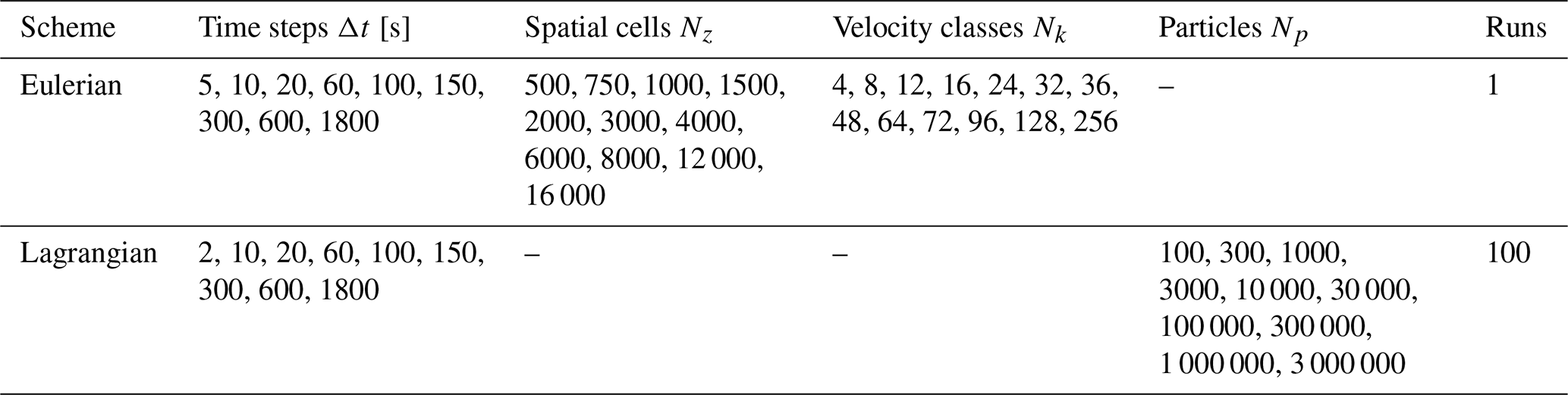
We present three different cases and simulate all three with both an Eulerian and a Lagrangian implementation of our model. Then, we compare the results and discuss convergence in terms of numerical parameters for both implementations. The cases are described below, and an overview of some aspects of the cases is presented in Table 1. Table 2 lists the numerical parameters we have used to investigate convergence.

Table 1 A brief summary of the boundary conditions (BCs) and reaction terms used in the three different cases.

Table 2 Numerical parameters used for convergence analysis. The same parameters are used in all three cases.

For case 1, we consider positively buoyant fish eggs with a distribution of rise speeds. Fish eggs will float to the surface but do not leave the water column; hence, we model these with a no-flux boundary condition at the surface (i.e. the particles cannot leave the water column).

For case 2, we consider microplastic particles with a velocity distribution that includes both rising and sinking particles, representing the diversity of densities associated with different polymer types. In this case, we again use a no-flux boundary at the surface, while the boundary at the seabed is zero flux in diffusion, though an advective flux is allowed to leave the domain. This represents negatively buoyant microplastic particles that are removed from the water column by settling onto the seabed.

For case 3, we consider oil which is entrained as droplets when a surface slick is broken up by waves. The droplets are all positively buoyant with the same density but have a size distribution which varies in time and which leads to a distribution of rising speeds. In this case, the boundary condition at the surface is zero diffusive flux, though an advective flux that represents droplets that merge with the surface slick is allowed. Additionally, we include the effect of entrainment of oil from the surface slick by breaking waves in our model.

A spatially variable diffusivity profile is used in all three cases. To calculate eddy diffusivity as a function of depth, we have used the GOTM turbulence model (Umlauf et al., 2005). The model was forced with a surface stress corresponding to a wind speed of 9 m s⁻¹ (Gill, 1982, p. 29), and it was run with a k-ω turbulence closure with a flux condition for turbulent kinetic energy (TKE) at the surface. The TKE flux at the surface accounts for wave breaking (Craig and Banner, 1994).

To support re-gridding and differentiation, an analytical expression has been fitted to the discrete diffusivity output from GOTM. In Fig. 1, the fitted analytical profile is shown together with the output from GOTM. The analytical expression is given by

$$\begin{array}{}\text{(17)}& K\left(z\right)=\mathit{\beta }(z_{\mathrm{0}}-z)\cdot e^{-\left(\mathit{\gamma }\right(z_{\mathrm{0}}-z){)}^{\mathit{\delta }}},\end{array}$$

where β=0.00636 m s⁻¹, γ=0.088 m⁻¹, δ=1.54, z₀=1.3 m, and z is negative downwards. The choice of using an analytical profile was mainly pragmatic: for the Lagrangian model, the diffusivity and its derivative must be evaluated at arbitrary positions; hence, some form of interpolation with continuous derivatives is needed in any case. Additionally, we made the profile non-zero at the surface, which seems physically reasonable for conditions with some wave breaking. Also, if the diffusivity is zero at the surface, positively buoyant particles would eventually get stuck at the surface, and this is not observed in surveys of e.g. fish eggs (Sundby, 1983).

Note that both implementations make use of the analytical diffusivity profile: in the Eulerian implementation, the diffusivity is given by the value of Eq. (17) evaluated at the cell boundaries, while for the Lagrangian implementation, Eq. (17) is evaluated at the position of each particle at each time step, and the derivative is evaluated by second-order central finite difference.

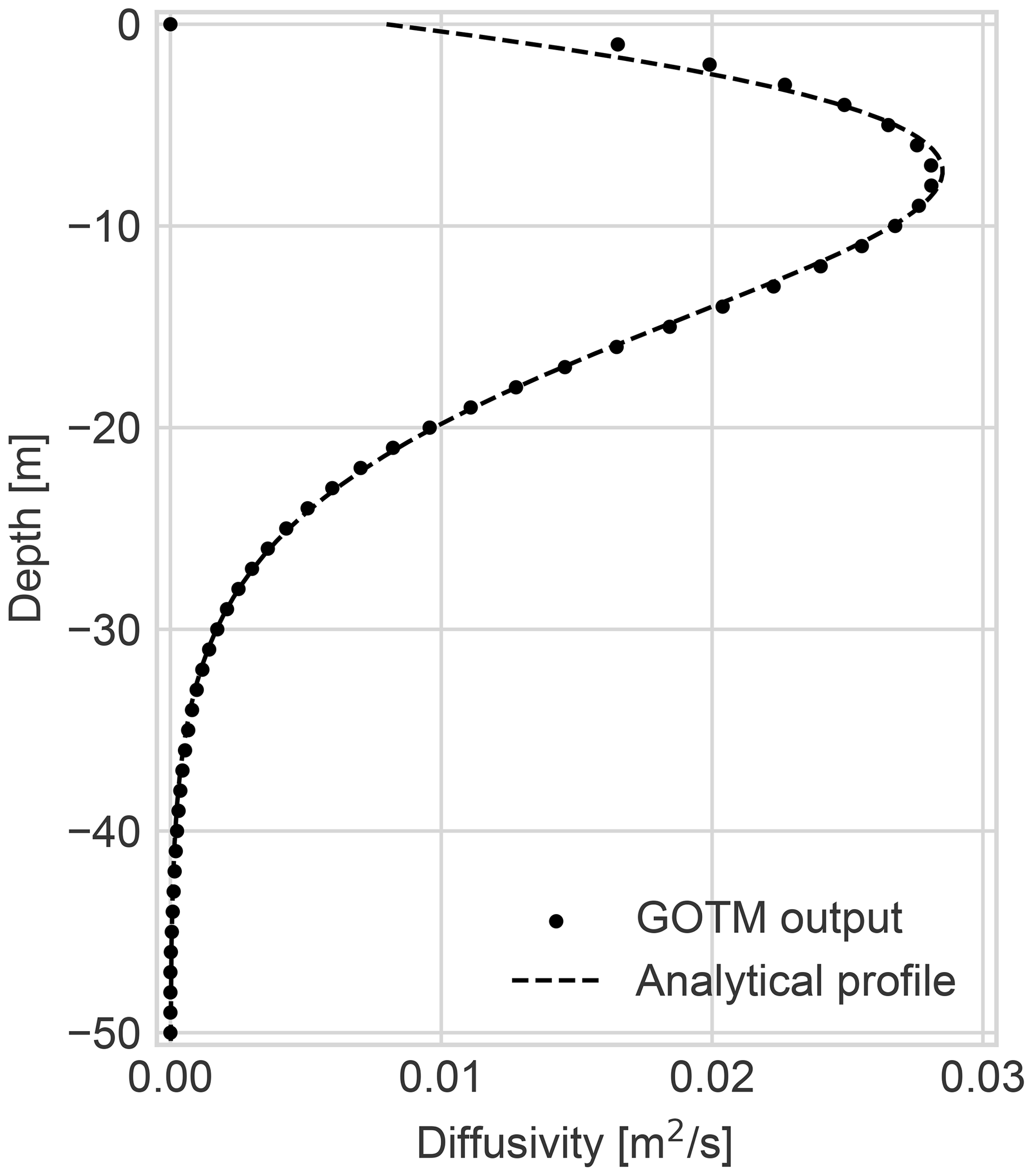
Figure 1 Eddy diffusivity output from a GOTM simulation, shown with the fitted analytical diffusivity profile used for the case studies.

For each of the three cases, our initial condition will be a submerged particle distribution. The spatial distribution will be a Gaussian distribution centred at −20 m depth, with a standard deviation of 4 m. The distribution of rise and settling speeds will be different for each case and will be explained in the description of each case below.

In all cases, we will present a direct comparison of the predicted total water column concentrations at different times from the Eulerian and the Lagrangian implementations. Total concentration in this case means that it is integrated over the velocity distribution, showing the total suspended concentration regardless of rising or settling velocity. Additionally, we show a numerical convergence analysis separately for the two schemes. For the Eulerian implementation, we consider the error to be a function of the number of velocity classes. For the Lagrangian implementation, we present the error as a function of the number of particles. As a measure of the error, we consider the first moment (the centre of mass) of the spatial concentration distribution (see Sect. 3.1.3 and 3.2.4). Additional numerical convergence tests are also presented in Appendix C.

4.1 Case 1: pelagic fish eggs

In case 1, we consider pelagic fish eggs with a distribution of rise velocities. These positively buoyant particles will rise towards the surface but do not form a surface slick. Rather, they rise to the surface in stagnant water but stay submerged and can be mixed back down by the eddy diffusivity (Sundby, 1983; Röhrs et al., 2014; Sundby and Kristiansen, 2015).

Taking an example from Sundby (1983, Table 3), we consider the eggs of the Arcto-Norwegian cod (Gadhus morhua L.), which is typically found to have a Gaussian distribution of terminal rise velocities with average $\overline{w}=\mathrm{0.96}$ mm s⁻¹ and a standard deviation of σ=0.38 mm s⁻¹. We furthermore assume that the distribution is truncated symmetrically about the mean such that $w\in [\overline{w}\pm \mathrm{2}\mathit{\sigma }]$. To divide this distribution into N_k velocity classes for use in the Eulerian implementation, we divide the interval $[\overline{w}\pm \mathrm{2}\mathit{\sigma }]$ into N_k sub-intervals with equal spacing Δw on a linear scale, and we calculate the mass fraction in each class, as described in Sect. 3.1.2. For the Lagrangian implementation, we sample the particle velocities at random from the truncated Gaussian distribution. Hence, a numerical particle may have any rise speed $w\in [\overline{w}\pm \mathrm{2}\mathit{\sigma }]$.

The results of our simulations for fish eggs are shown in Fig. 2. In panel (a), concentration profiles are shown for four different times (including t=0), with the Lagrangian results shown as continuous lines and the Eulerian results for the same times shown as dashed black lines. The concentration profiles from the Eulerian implementation were produced with time step Δt_E=10 s, N_k=128 classes, and N_z=8000 spatial cells, while the Lagrangian results used time step Δt_L=10 s and $N_p=\mathrm{3}\times {\mathrm{10}}^{\mathrm{6}}$ particles converted to a concentration by bin count for 8000 bins. We observe that the two implementations produce essentially identical predicted concentrations.

In panel (b) of Fig. 2, we show the convergence of the Eulerian results with the number of velocity classes, with the other numerical parameters kept constant at time step Δt_E=10 s and N_z=8000 spatial grid cells. The plot shows the error in the first moment, where the error is calculated relative to a reference solution from a simulation with N_k=256 classes. We observe that the convergence with the number of classes appears to be of order 2, with the error going down as $\mathrm{1}/N_k^{\mathrm{2}}$.

Finally, in panel (c), we show the convergence of the Lagrangian results as a function of the number of particles N_p, keeping a fixed time step of Δt_L=10 s. The figure shows the standard deviation of the modelled first moment, calculated over an ensemble of 100 simulations for each value of N_p. As noted above, the first moment is just the average particle position, and as expected from the Lindeberg–Lévy theorem, the standard deviation of the first moment goes down as $\mathrm{1}/\sqrt{N_p}$ (see Sect. 2.6).

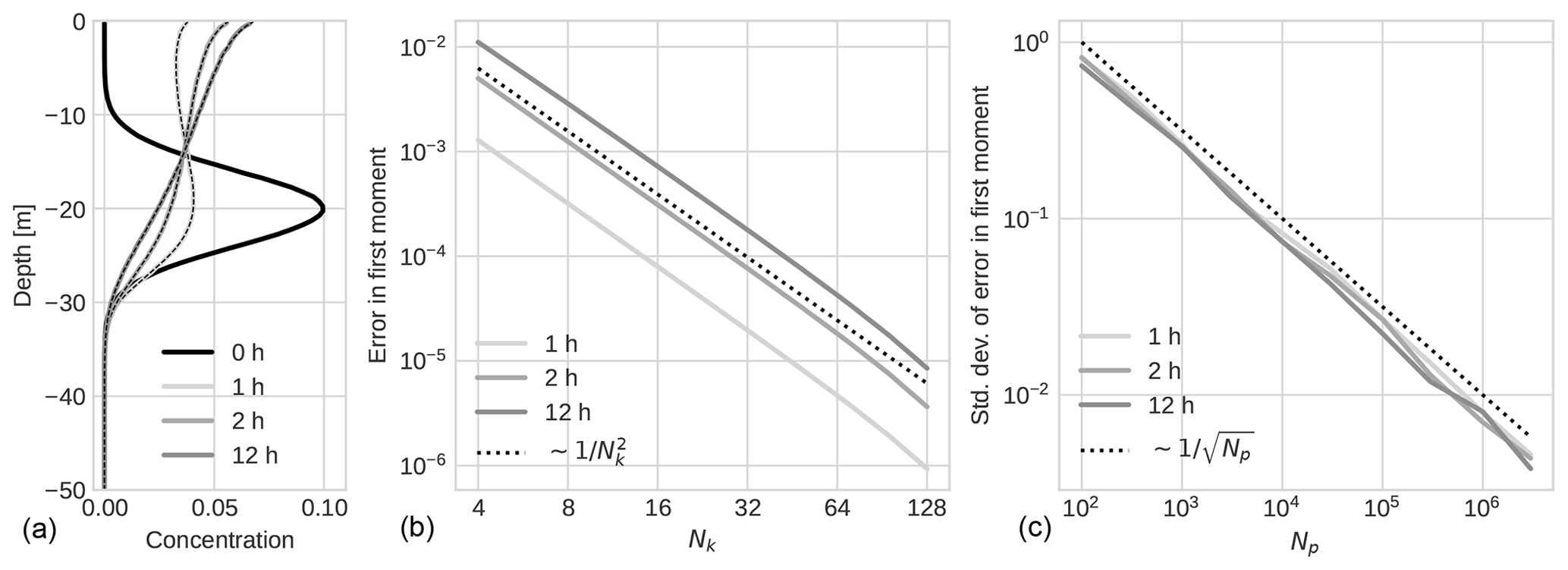
Figure 2 Results for case 1: fish eggs. Panel (a) shows concentration profiles at different times, with Lagrangian results shown as continuous lines and Eulerian results for the same times shown as dashed black lines. (b) Convergence of the error in the first moment for the Eulerian results as a function of the number of velocity classes. (c) Convergence of the standard deviation of the first moment for the Lagrangian results as a function of the number of particles.

4.2 Case 2: microplastics

In this case, we consider a distribution of microplastic particles. As the only parameter describing the numerical particles in our model is the terminal rise and settling velocities, we have obtained a velocity distribution based on published descriptions of microplastics.

As our starting point, we consider particles with a distribution of densities from 0.8 to 1.5 kg L⁻¹, a distribution of sizes from 20 µm to 5 mm, and a distribution of shapes described by the Corey shape factor. We assume the density of seawater to be 1.025 kg L⁻¹. The distributions of density, size, and shape are taken from Kooi and Koelmans (2019). The terminal rise and settling velocities of these particles are calculated from empirical relations obtained by Waldschläger and Schüttrumpf (2019), which give terminal velocities as a function of density, size, and shape. To obtain a distribution of velocities, we used a Monte Carlo method that consists of generating a large number of random combinations of density, size, and shape, drawn from the distributions given in Kooi and Koelmans (2019), and mapping those to velocities via the relationships given by Waldschläger and Schüttrumpf (2019).

For the Eulerian simulations, discretisations of the velocity distribution into different numbers of classes were obtained as histograms with different numbers of bins of 10⁹ randomly generated terminal velocities. For the Lagrangian simulations, the terminal velocities of the particles were obtained by directly generating random velocities as described above. A detailed description of the steps involved in obtaining the terminal velocities for microplastics is given in Appendix B. See also Isachenko (2020) for another example of a similar approach.

In this case, particles are allowed to leave the water column via the seafloor at 50 m depth, where we enforce zero diffusive flux while allowing the advective flux to carry particles across the boundary. This represents particles that leave the water column (and thus the simulation) by settling onto the seafloor, where they are no longer able to be resuspended by the eddy diffusivity. Different resuspension mechanisms can of course be included in the model, but we have chosen to ignore that here.

The results of our simulations for microplastics are shown in Fig. 3. In panel (a), concentration profiles are shown for four different times, with the Lagrangian results shown as continuous lines and the Eulerian results for the same times shown as dashed black lines. As in case 1, the concentration profiles from the Eulerian implementation were produced with time step Δt_E=10 s, N_k=128 classes, and N_z=8000 spatial cells, while the Lagrangian results used time step Δt_L=10 s and $N_p=\mathrm{3}\times {\mathrm{10}}^{\mathrm{6}}$ particles converted to concentration by bin count for 8000 bins. Again, we observe that the two implementations give very similar predictions as the curves are visually indistinguishable.

In panel (b), we show the convergence of the first moment in the Eulerian results as a function of the number of classes. The $\mathrm{1}/N_k^{\mathrm{2}}$ trend is less clear than in case 1, and the size of the error appears to be somewhat sensitive to the number of classes – for example, 32 classes give a smaller error than 36 classes for two of the times considered.

In panel (c), we show the convergence with the number of particles of the standard deviation of the first moment for the Lagrangian implementation. Again, as expected from the discussion in Sect. 2.6, this follows a $\mathrm{1}/\sqrt{N_p}$ trend.

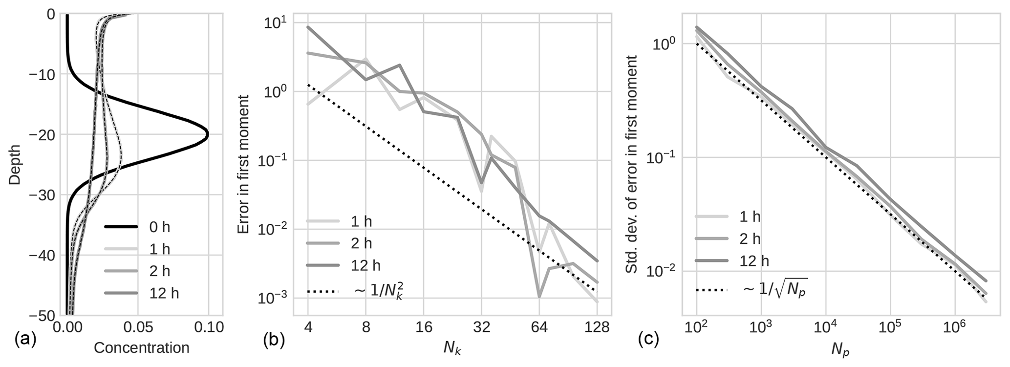
Figure 3 Results for case 2: microplastics. Panel (a) shows concentration profiles at different times, with Lagrangian results shown as continuous lines and Eulerian results for the same times shown as dashed black lines. (b) Convergence of the error in the first moment for the Eulerian results as a function of the number of velocity classes. (c) Convergence of the standard deviation of the error in the first moment for the Lagrangian results as a function of the number of particles.

In contrast to case 1, here we have particles with both positive and negative terminal velocities. As the particles are allowed to leave the water column, the total mass in suspension (i.e. the integral of the concentration profile) decreases with time. Hence, we also present the remaining suspended mass as a function of time. Panel (a) of Fig. 4 shows the remaining mass fraction suspended in the water column for both implementations, while panel (b) shows the difference between the two implementations for 10 different Lagrangian runs. The oscillatory nature of the difference is due to the randomness of the stochastic Lagrangian particle model. The results were produced with the same numerical parameters as stated in the previous paragraph.

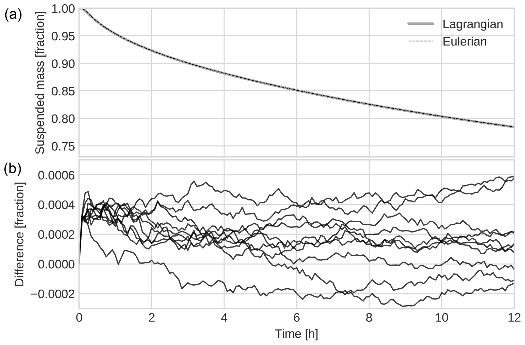
Figure 4 (a) Remaining suspended mass as a function of time for the microplastic case for both the Eulerian and the Lagrangian implementation. (b) The difference between the suspended mass fractions of the two models for 10 different runs of the Lagrangian implementation.

4.3 Case 3: oil droplets with breaking-wave entrainment

In this case, we consider a simplified one-dimensional oil spill model, which includes entrainment of surface oil by breaking waves; rising of oil droplets due to buoyancy; turbulent diffusive mixing; and oil droplets rising to the surface, creating a surface slick. As the entrainment mechanism is unique to this case, it is described in some detail below.

To model the entrainment of surface oil by breaking waves, we need the entrainment rate, the entrainment depth, and the size distribution of the entrained droplets. We model entrainment as a first-order decay process (Johansen et al., 2015):

$$\begin{array}{}\text{(18)}& {\displaystyle \frac{\mathrm{d}{Q}_{\mathrm{s}}}{\mathrm{d}t}}=-\mathit{\alpha }{Q}_{\mathrm{s}},\end{array}$$

where Q_s is the amount of oil at the surface, and α is the entrainment rate coefficient. The coefficient α is calculated according to Li et al. (2017). For the entrainment depth, we use the classic result by Delvigne and Sweeney (1988), where the entrained oil is evenly distributed across the interval

$$\begin{array}{}\text{(19)}& \mathrm{1.15}{H}_{\mathrm{s}}<z<\mathrm{1.85}{H}_{\mathrm{s}}.\end{array}$$

H_s is the significant wave height, here assumed to be 1.74 m. The size distribution of the entrained droplets is also taken from Johansen et al. (2015) using modified Weber number scaling. The size distribution is log-normal, with a fixed-width parameter and a median size d₅₀, which depends on the wave height and the properties of the oil. For a detailed description of this scheme, as well as of the values of the relevant oil properties used here, see Nordam et al. (2019b).

From Eq. (18), we see that the entrainment rate depends on the amount of oil at the surface. Since all the oil in this model is either submerged or at the surface, the amount of oil in the surface slick at time t, Q_s(t), can be found as follows:

$$\begin{array}{}\text{(20)}& Q_{\mathrm{s}}\left(t\right)=Q_{\mathrm{tot}}-\underset{\mathrm{0}}{\overset{H}{\int }}C(z,t)\mathrm{d}z,\end{array}$$

where Q_tot is the total amount of oil present.

Using uniform entrainment throughout the interval $z\in [\mathrm{1.15}{H}_{\mathrm{s}},\mathrm{1.85}{H}_{\mathrm{s}}]$ (Delvigne and Sweeney, 1988), we find the source term in the Eulerian advection–diffusion–reaction equation from the entrainment rate and the length of the entrainment interval:

$$\begin{array}{}\text{(21)}& \begin{array}{rl}& S(z,C(z,t_n\left)\right)=\\ & \left\{\begin{array}{ccc}\mathit{\alpha }\frac{Q_{\mathrm{s}}\left(t_n\right)}{\mathrm{0.7}{H}_{\mathrm{s}}}& \mathrm{if}& \mathrm{1.15}{H}_{\mathrm{s}}<z<\mathrm{1.85}{H}_{\mathrm{s}},\\ \mathrm{0}& \mathrm{otherwise}.& \end{array}\right.\end{array}\end{array}$$

In the Lagrangian implementation, we use the approximation that the analytical solution of Eq. (18) for constant α is an exponential decay with lifetime $\mathit{\tau }=\mathrm{1}/\mathit{\alpha }$. This means we submerge a fraction of the surface slick at every time step, with that fraction being given by

$$\begin{array}{}\text{(22)}& p=\mathrm{1}-{\mathrm{e}}^{-\mathrm{\Delta }t/\mathit{\tau }}.\end{array}$$

Thus, entrainment is implemented as a stochastic process where particles that have surfaced are re-entrained with probability p at every time step. If entrained, a particle is assigned a depth drawn from a uniform random distribution at the interval $z\in [\mathrm{1.15}{H}_{\mathrm{s}},\mathrm{1.85}{H}_{\mathrm{s}}]$ and a random size drawn from the log-normal size distribution described above.

Surfacing of oil droplets is described as a boundary condition where an advective flux is allowed to pass through the boundary at the surface while enforcing zero diffusive flux, as described in Sect. 2.4. For additional details on the implementation of surfacing and entrainment of oil in a Lagrangian model, see also Nordam et al. (2019a, b).

The results of our simulations for oil droplets are shown in Fig. 5. In panel (a), concentration profiles are shown for four different times, with the Lagrangian results shown as continuous lines and the Eulerian results for the same times shown as dashed black lines. As in cases 1 and 2, the concentration profiles from the Eulerian implementation were produced with time step Δt_E=10 s, N_k=128 classes, and N_z=8000 spatial cells, while the Lagrangian results used time step Δt_L=2 s and $N_p=\mathrm{3}\times {\mathrm{10}}^{\mathrm{6}}$ particles converted to concentration by bin count for 8000 bins.

In panel (b), we show the convergence of the Eulerian results as a function of the number of classes. As in case 1, the error scales with $\mathrm{1}/N_k^{\mathrm{2}}$, though here, the absolute value of the error is about 2 orders of magnitude larger. Panel (c) shows the convergence of the Lagrangian results with the number of particles, which, as before, follows the $\mathrm{1}/\sqrt{N_p}$ trend closely.

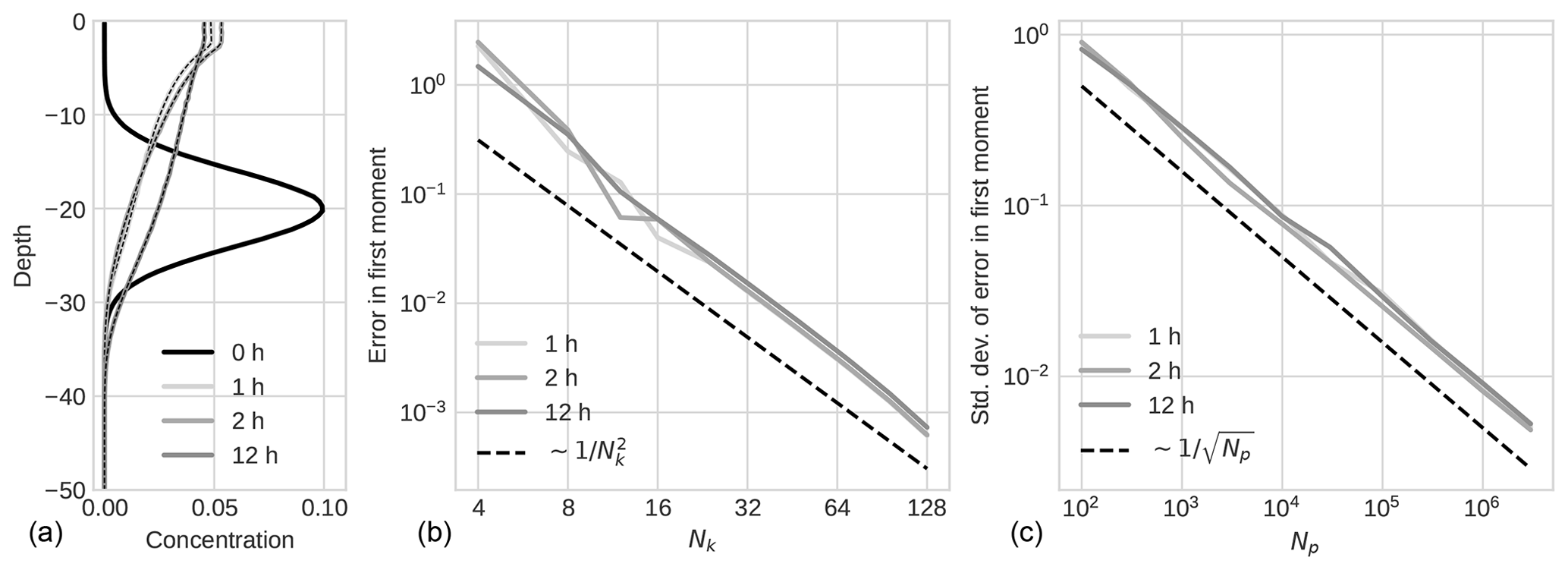
Figure 5 Results for case 3: oil droplets with entrainment. Panel (a) shows concentration profiles at different times, with Lagrangian results shown as continuous lines and Eulerian results for the same times shown as dashed black lines. (b) Convergence of the error in the first moment for the Eulerian results as a function of the number of velocity classes. (c) Convergence of the standard deviation of the first moment for the Lagrangian results as a function of the number of particles.

The total amount of submerged oil changes in time as oil droplets surface and are re-entrained. Over time, the submerged size distribution shifts towards smaller droplets as these take longer to reach the surface, causing the centre of mass to shift downwards over time. As before, the two schemes give very similar results. As for case 2, we also present here the remaining suspended mass as a function of time. Panel (a) of Fig. 6 shows the remaining mass fraction suspended in the water column for both implementations, while panel (b) shows the difference between the implementations for 10 different runs of the Lagrangian implementation. The oscillatory nature of the difference is due to the randomness of the stochastic Lagrangian particle model. The results were produced with the same numerical parameters as stated in the previous paragraph.

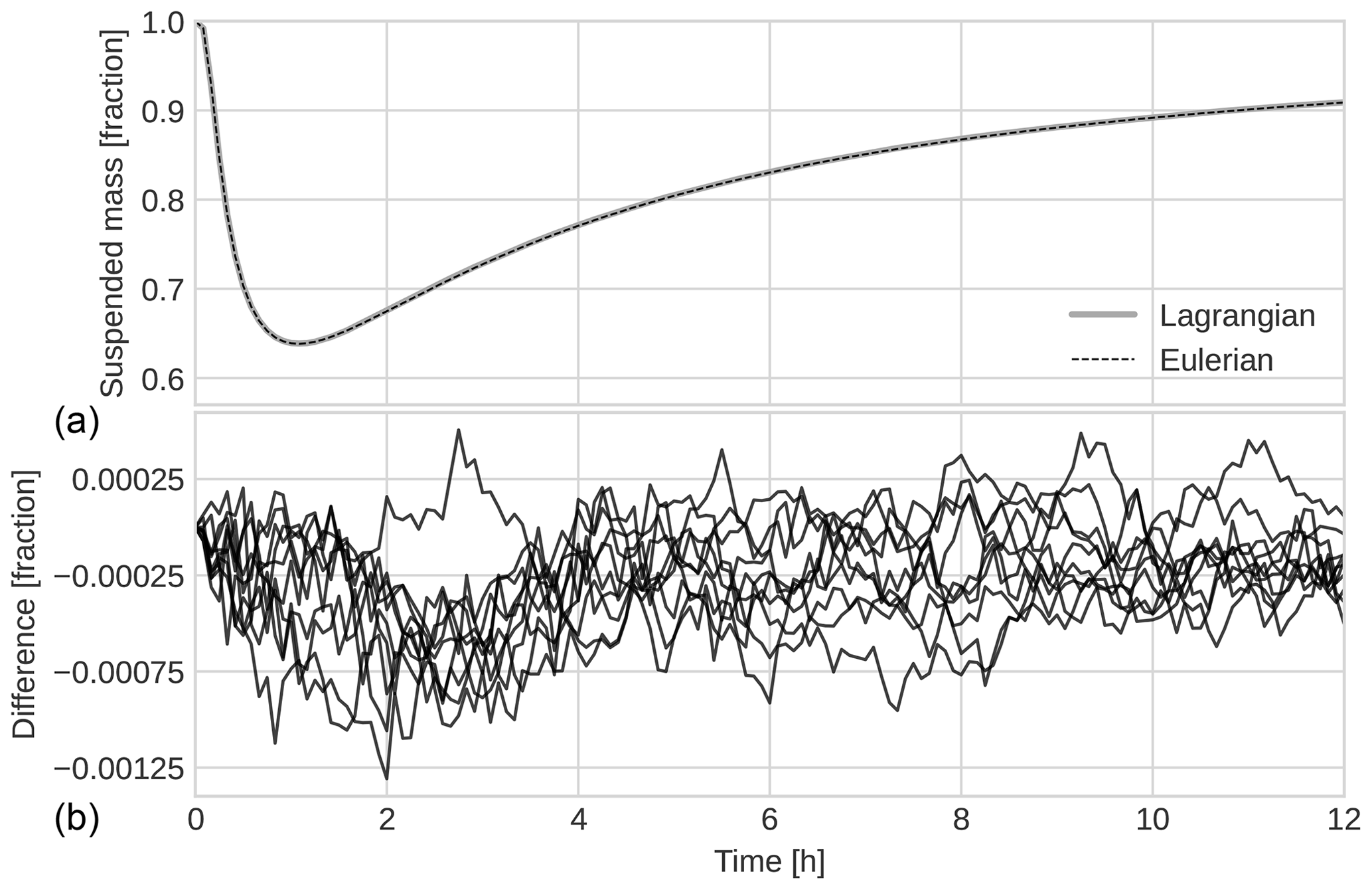
Figure 6 (a) Remaining suspended mass as a function of time for the oil case for both the Eulerian and the Lagrangian implementation. (b) The difference between the suspended mass fractions of the two models.

5 Discussion

In this paper, we have conducted a comparison of an Eulerian and a Lagrangian implementation of a water column model for particles with different distributions of rising and sinking speeds. To highlight different choices of boundary conditions and a reaction term, we have chosen to use fish eggs, microplastics, and oil droplets as our example cases. The model can also easily be applied to other cases, such as mineral particles, nanoparticles, algae, and chemicals. More complex reaction terms, such as agglomeration, can also be added to the same modelling framework.

5.1 Boundary conditions

Boundary conditions are always an essential part of the problem for any model based on PDEs, and indeed, the boundary conditions must be specified before the problem can be said to be well posed (Gustafsson, 2008, Chap. 2). The implementation of different boundary conditions in Eulerian models is amply addressed in the applied numerical literature (see e.g. Hundsdorfer and Verwer, 2003; Versteeg and Malalasekera, 2007). Hence, any Eulerian models for environmental transport problems may draw on a wide body of standard reference works describing the implementation of different boundary conditions.

Transport modelling with stochastic particle methods, on the other hand, is perhaps more of a niche endeavour, and there exists less general applied literature on the topic of numerical methods for SDEs compared to PDEs. The standard reference on numerical solution of SDEs, Kloeden and Platen (1992)¹, does not directly address the question of boundary conditions but mentions a few references in the section on bibliographical notes (Kloeden and Platen, 1992, pp. 593–594). These are all of a rather technical nature.

In the mathematical literature, an Itô diffusion (of which Eq. 2 is an example) on a domain with a reflecting boundary is known as a Skorokhod problem, after the Ukrainian mathematician Anatoliy V. Skorokhod, who wrote two early papers on the topic (Skorokhod, 1961, 1962). In particular, Skorokhod (1961) describes how an SDE with a reflecting boundary can be formally described by adding a term which is zero everywhere except on the boundary and which causes any trajectory that touches the boundary to be immediately reflected. However, the focus of that paper was on proving the existence and uniqueness of solutions to this modified system and not on numerical solutions.

In the applied literature on atmospheric transport modelling with random flight models, the issue of boundary conditions has received some attention (see e.g. Wilson and Flesch, 1993, and Rodean, 1996, Chap. 11). Less has been written about boundary conditions in the applied literature on random walk models, which are more commonly used in applied oceanography. For reflecting boundary conditions, a pragmatic and common choice is to simply take any particles that have been randomly displaced to a point outside the boundary and to reflect them to an equal distance inside the boundary (see e.g. Israelsson et al., 2006). This approach has also been shown to be exact in the special case of no advection and constant diffusivity (Gillespie and Seitaridou, 2012, pp. 58–60 and 75–76). In the more general case of variable diffusivity, some details are discussed in Ross and Sharples (2004), including a numerical artifact that appears when the diffusivity has a non-zero derivative at the boundary. Nordam et al. (2019a) discuss the separate treatment of boundary conditions for advection and diffusion and conduct a numerical comparison with Neumann and Robin boundary conditions in an Eulerian scheme. In this paper, we have used the same approach as in Nordam et al. (2019a).

We have provided a detailed description of our implementation of two different types of boundary conditions in the Lagrangian scheme. While our implementation may not have a rigorous foundation in the theory of SDEs, we do present a comparison between our Lagrangian and Eulerian implementations, where the Eulerian method uses a standard approach for FVMs. In cases 2 and 3 (microplastics and oil droplets), we show that the two implementations give very similar predictions of the amount of mass which remains suspended in the water column as a function of time, which of course indicates that the net effect of the boundary conditions is the same in the two implementations. For an additional discussion of this topic, see also Nordam et al. (2019a).

5.2 Convergence of numerical results

We have paid special attention to the representation of particles with a distribution of terminal rising and settling velocities. In a Lagrangian particle model, a distribution of terminal velocities may be straightforwardly represented since each numerical particle can have its own velocity. In an Eulerian model, we have to introduce discrete classes with different velocities to represent the true distribution. We have investigated how the error is reduced with an increasing number of particles and classes respectively.

As a measure of the error in the Lagrangian implementation, we have used the standard deviation of the first moment of the position distribution, M₁ (i.e. the centre of mass). As is usual for a Monte Carlo method, the standard deviation of M₁(N_p) goes down proportionally to $\mathrm{1}/\sqrt{N_p}$, where N_p is the number of particles. If the particles can be considered as independent samples, this behaviour follows from the Lindeberg–Lévy theorem, as discussed in Sect. 2.6. We note, however, that the usual $\mathrm{1}/\sqrt{N_p}$ scaling also seems to be followed very closely in case 3, where the particles cannot strictly be said to represent independent samples due to the inclusion of a distribution-dependent reaction term.

For the Eulerian implementation, we have considered the error in the modelled first moment M₁(N_k) as a function of the number of classes N_k used to discretise the velocity distribution representing the particles. We found that the error scales as $\mathrm{1}/N_k^{\mathrm{2}}$, where the velocity of each class is represented by the midpoint of the interval spanned by the class. To the best of our knowledge, this result has not previously been published in this context. Models where a distribution of velocities (e.g. due to a distribution of sizes) is represented by a finite number of discrete classes are often used in both marine and atmospheric transport modelling (see e.g. Tegen and Lacis, 1996; Zender et al., 2003; Wichmann et al., 2019; Cui et al., 2020). Hence, additional understanding of how the number of velocity classes affects the accuracy of predictions should be of some interest within these fields.

We note, however, that the result showing $\mathrm{1}/N_k^{\mathrm{2}}$ scaling of the error is perhaps not so surprising. Consider as an example the mean of a velocity distribution p(v), which is given by

$$\begin{array}{}\text{(23)}& \overline{v}=\underset{-\mathrm{\infty }}{\overset{\mathrm{\infty }}{\int }}vp\left(v\right)\mathrm{d}v.\end{array}$$

If the integral is evaluated numerically, there will be a numerical error, which will depend on the chosen approach. Our approach has been to divide the underlying velocity distribution into equal-sized bins and to let each bin be represented by its midpoint (on either linear or logarithmic scales, depending on the case). This is equivalent to the midpoint quadrature method, which is known to have an error proportional to Δx², where Δx is the bin size (Wendroff, 1969, p. 23). This, in turn, is of course proportional to $\mathrm{1}/N_k^{\mathrm{2}}$, where N_k is the number of bins.

5.3 Relative merits of Eulerian and Lagrangian methods

Numerous studies have discussed different aspects and applications of Lagrangian and Eulerian methods and have compared the two approaches (see e.g. Fay et al., 1995; Benson et al., 2017; Nordam et al., 2019a; Nepstad et al., 2022). Here, we consider the question of which implementation should be preferred when modelling particles with a distribution of rising or settling speeds.

First we consider case 1, in which we modelled positively buoyant fish eggs with a Gaussian distribution of terminal rise velocities. For the Eulerian implementation, the numerical error in the first moment due to a finite number of velocity bins starts out between 0.01 and 0.001 m for N_k=4 size classes and reduces very consistently as $\mathrm{1}/N_k^{\mathrm{2}}$ from there (see Fig. 2). A numerical error of less than 0.01 m in the position of the centre of mass is clearly far smaller than the error due to other uncertainties and model approximations. Hence, with such a well-behaved velocity distribution in this particular case, an Eulerian model with a small number of velocity classes will give more than adequate numerical accuracy.

For the Lagrangian implementation, on the other hand, we need to use 10⁶ particles to reach an error of about 0.01 m, a result of the slower $\mathrm{1}/\sqrt{N_p}$ convergence. For modelling fish eggs in a water column model, an Eulerian approach seems to be the most efficient choice in terms of the balance between error and computational effort. This is not necessarily the case in a full three-dimensional model due to the computational effort involved in tracking the concentration fields for the individual velocity classes across the entire computational domain.

In case 2 with the microplastics, we have a more complicated velocity distribution. The positive and negative parts of the distribution are shown separately on log scales in Fig. B1, where we see that the positively buoyant part of the distribution is bimodal. Due to the very wide range of velocities present, we chose to use log-spaced velocity bins (separate for positive and negative velocities) in the Eulerian implementation. Nevertheless, we see from Fig. 3 that the error in the first moment shows some oscillation with the changing number of classes. We also note that the absolute value of the error is far higher than in case 1, and we need around 64 velocity classes to reach an error of 0.01 m in the modelled first moment M₁(N_k). Compare this to case 1, where the same accuracy was achieved with only four classes.

For the Lagrangian implementation, the results of case 2 look far more similar to those of case 1, and we find that 10⁶ to 3×10⁶ particles will yield a sampling error of 0.01 m. In the one-dimensional case, the Eulerian implementation is still more efficient than the Lagrangian implementation, but in three dimensions, this is probably no longer the case. The results will, of course, depend on parameters such as time step, grid resolution, and the choice of numerical solver. However, it is clear that the computational effort of solving the advection–diffusion equation for 64 individual velocity classes is considerable.

In case 3 with the oil droplets, we consider a simplified one-dimensional oil spill model. Lagrangian approaches have a long history in oil spill modelling, both for horizontal transport (Tayfun and Wang, 1973) and vertical transport (Elliott et al., 1986). A critical issue in oil spill modelling is that the droplet size distribution is both broad and changing over time. This is easily modelled with a Lagrangian approach, while an Eulerian approach might require either some form of dynamic size class scheme or a very large number of size classes. From panel (b) of Fig. 5, we see that the error in the first moment starts at a little above 1 m for N_k=4 classes and goes down fairly consistently as $\mathrm{1}/N_k^{\mathrm{2}}$. As such, the scaling is very similar to case 1, while the prefactor is again 2–3 orders of magnitude larger, and an error of 0.01 m is achieved with N_k=32 classes. The Lagrangian approach, on the other hand, behaves quite similarly to cases 1 and 2 and reaches an error of 0.01 m with 10⁶ particles.

It is important to point out that the errors discussed above are of different natures for the Eulerian and the Lagrangian implementations. In the Eulerian approach, solving with a finite number of speed classes, N_k, leads to a systematic error that goes to zero as N_k→∞. In contrast, a finite number of particles, N_p, leads to a stochastic sampling error in the Lagrangian approach. If the particles are independent, the sampling error is not systematic, and when N_p→∞, the standard deviation of the sample error goes to zero as $\mathrm{1}/\sqrt{N_p}$. See also a further discussion on this point in Sect. 2.6 and Appendix C.

6 Conclusions

In this paper, we have implemented and compared two different versions of a water column model for particles that undergo diffusion and that rise or sink with different distributions of terminal velocities. Our Eulerian implementation used discrete velocity classes to represent the velocity distribution, while the Lagrangian implementation allowed each particle to have its own velocity.

We have studied the rate of convergence of the two different implementations considering the centre of mass (i.e. the first moment of the concentration profile) as a measure of the error. Our main interest has been to show that we can implement different boundary conditions in an equivalent manner in the two schemes and to demonstrate how the numerical error is reduced with an increasing number of velocity classes and particles for the Eulerian and Lagrangian implementations respectively. Convergence results for varying time steps and (in the Eulerian case) spatial resolutions are also shown in Appendix C.

Three different example cases were considered: positively buoyant fish eggs with a Gaussian velocity distribution, microplastics with a distribution of positive and negative velocities obtained by means of a Monte Carlo approach (see Appendix B), and positively buoyant oil droplets with a time-varying velocity distribution. In all three cases, we find that the stochastic sampling error in the Lagrangian method scales as $\mathrm{1}/\sqrt{N_p}$ (where N_p is the number of particles) with about the same prefactor for all cases. Interestingly, this also appears to hold in the case of oil droplets, where the particles cannot strictly be said to be independent samples.

For the Eulerian implementation, we find that the error appears to scale as $\mathrm{1}/N_k^{\mathrm{2}}$ (where N_k is the number of velocity classes), though the prefactor varies by several orders of magnitude between the cases. We also see that, in the case of microplastics, the exact choice of the velocity classes has a significant impact on the error, possibly due to the multi-modal nature of the velocity distribution.

Owing to current shear and density gradients, vertical behaviour is very important for correctly modelling horizontal transport in the ocean. While it might be hard to draw strict conclusions about three-dimensional simulations from one-dimensional examples, we would still argue that a one-dimensional model captures a large part of the complexity of modelling particle distributions: horizontal advection and diffusion affect all particles equally, and the differences in vertical behaviour are well represented in a water column model. Hence, it is clear from our results that the number of classes needed to get accurate results in an Eulerian simulation will depend strongly on the velocity distribution of the relevant particles. We observed that far fewer classes were needed for the fish egg case with a Gaussian velocity distribution than for the microplastic case, which used a wider, multi-modal distribution. Similarly, the time-dependent size distribution (and thus velocity distribution) seen in the oil case needed more classes to give accurate results than the fish egg case. Hence, our results would suggest that Lagrangian particle models have a particular advantage when wider, less normal velocity distributions are considered or when the size distribution changes with time.

Appendix A: Additional implementation details

A1 Eulerian implementation

A1.1 Discretisation

The advection–diffusion–reaction (ADR) equation describes how the concentration C_k of a substance affected by diffusive, advective, and reactive processes develops in time. In this study, we consider the one-dimensional version of the ADR equation and consider vertical motion only. The diffusivity is assumed to be a function of position. Similarly, the advection velocity, which here represents particles rising or sinking due to buoyancy, may also be spatially dependent such that particles stop at the surface and/or bottom boundaries. Finally, the reaction term is assumed to depend on both concentration and position. Consequently, Eq. (1) with all dependencies explicitly shown becomes

$$\begin{array}{}\text{(A1)}& \begin{array}{rl}{\displaystyle \frac{\partial C_k(z,t)}{\partial t}}& ={\displaystyle \frac{\partial }{\partial z}}\left(K\left(z\right){\displaystyle \frac{\partial C_k(z,t)}{\partial z}}\right)\\ & -{\displaystyle \frac{\partial }{\partial z}}\left(w_k\right(z\left)C_k\right(z,t\left)\right)\\ & +S(z,C_{\mathrm{1}}(z,t),\mathrm{\dots },C_{N_k}(z,t\left)\right),\end{array}\end{array}$$

where C_k(z,t) is the concentration of the material of class k, K(z) is the spatially dependent diffusivity, w_k(z) is the spatially dependent velocity of the material in class k, $S(z,C_{\mathrm{1}}(z,t),\mathrm{\dots },C_{N_k}(z,t\left)\right)$ is the source term (which may depend on the concentration of all classes), and N_k is the number of classes.

In finite-volume methods (FVMs), the PDE is converted to an integral form by integration over control volumes or cells. As illustrated in Fig. A1, cell centres are given integer indices, and cell faces are given half-integer indices such that cell j extends from $z_{j-\mathrm{1}/\mathrm{2}}$ to $z_{j+\mathrm{1}/\mathrm{2}}$, with the cell width being equal to Δz_j. Considering a spatially discretised version of Eq. (A1), we use the divergence theorem to write the volume integrals of the terms on the right-hand side as surface integrals over the cell faces. By applying the Leibniz integral rule to change the order of the spatial integral and the differentiation with respect to time on the left-hand side, the average concentration of class k in cell j, ${\stackrel{\mathrm{‾}}{C}}_{k,j}$, may be defined. Similarly the average reaction term for class k in cell j, ${\stackrel{\mathrm{‾}}{S}}_{k,j}$, is found by integration.

The integral form of Eq. (A1) for the average concentration of the material of class k in cell j thus reads as

$$\begin{array}{}\text{(A2)}& \begin{array}{rl}\mathrm{\Delta }{z}_j{\displaystyle \frac{\mathrm{d}{\stackrel{\mathrm{‾}}{C}}_{k,j}}{\mathrm{d}t}}& =(K{\displaystyle \frac{\partial C_k}{\partial z}}{)}_{j+\frac{\mathrm{1}}{\mathrm{2}}}-(K{\displaystyle \frac{\partial C_k}{\partial z}}{)}_{j-\frac{\mathrm{1}}{\mathrm{2}}}\\ & -(w_k{C}_k{)}_{j+\frac{\mathrm{1}}{\mathrm{2}}}+(w_k{C}_k{)}_{j-\frac{\mathrm{1}}{\mathrm{2}}}+\mathrm{\Delta }{z}_j{\stackrel{\mathrm{‾}}{S}}_{k,j},\end{array}\end{array}$$

where the subscripts on the brackets indicate where the variables are evaluated, e.g. $(w_k{C}_k{)}_{j+\mathrm{1}/\mathrm{2}}=w_k(z_{j+\mathrm{1}/\mathrm{2}}\left)C_k\right(z_{j+\mathrm{1}/\mathrm{2}})$. This is noted to be an exact equation for the rate of change of the cell-averaged concentrations, ${\overline{C}}_{k,j}$, given in terms of the advective and diffusive fluxes through the cell faces, and of the cell-average source term. The fact that the concentration within a cell is explicitly expressed as the sum of the fluxes into and out of the cell gives the FVM its mass-conserving properties (in the case when S=0).

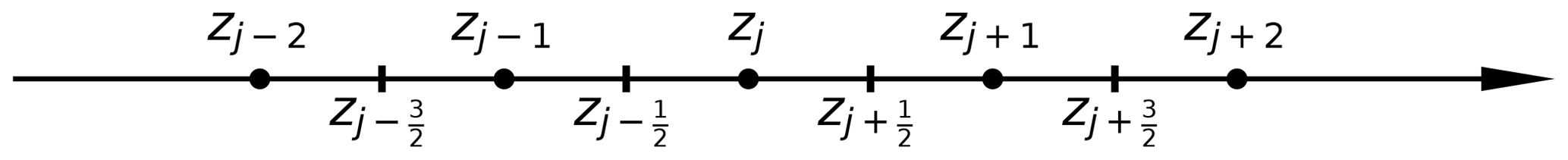
Figure A1 Illustration of the discretisation of the z axis in the Eulerian implementation. Concentrations are calculated at cell centres (marked with round dots) with integer indices, while fluxes are calculated through cell faces (marked with vertical ticks) at half-integer indices.

Next, we make an approximation by assuming the concentration to be constant within each control volume such that the cell averages ${\stackrel{\mathrm{‾}}{C}}_{k,j}$ and ${\stackrel{\mathrm{‾}}{S}}_{k,j}$ may be approximated by the values located at the cell centres. The concentration and source term at z_j are denoted by C_k,j and S_k,j respectively. Choosing a constant grid spacing Δz, the z axis is discretised into $N_z=H/\mathrm{\Delta }z$ equally sized cells, where H is the length of the domain. For another example of a similar derivation, see Versteeg and Malalasekera (2007, pp. 243–246).

A1.2 Numerical approximation of fluxes

In Eq. (A2), the first two terms on the right represent the diffusive fluxes through the faces of cell j, and the next two terms represent the advective fluxes. The diffusive fluxes at the cell faces are approximated by a second-order central difference of the two adjacent cells (see e.g. Versteeg and Malalasekera, 2007, p. 117) – that is, in the form

$$\begin{array}{}\text{(A3)}& \begin{array}{rl}(K{\displaystyle \frac{\partial C_k}{\partial z}}{)}_{j+\frac{\mathrm{1}}{\mathrm{2}}}& \approx K_{j+\frac{\mathrm{1}}{\mathrm{2}}}{\displaystyle \frac{C_{k,j+\mathrm{1}}-C_{k,j}}{z_{j+\mathrm{1}}-z_j}}\\ & =K_{j+\frac{\mathrm{1}}{\mathrm{2}}}{\displaystyle \frac{C_{k,j+\mathrm{1}}-C_{k,j}}{\mathrm{\Delta }z}},\end{array}\end{array}$$

where the diffusivity K_j+½ is determined on the cell faces either explicitly by an analytic expression, if available, or by interpolation in the case of a discrete diffusivity.

For the advective fluxes, however, linear numerical schemes of second-order accuracy and higher are known to yield numerical oscillations for advection-dominated problems (i.e. $Pe=\frac{\left|v\right|\mathrm{\Delta }z}{K}\gg \mathrm{1}$) for non-smooth solutions (Hundsdorfer and Verwer, 2003, pp. 66–67, 118–119). To be able to handle advection-dominated cases, we implemented a more flexible second-order numerical scheme for advection. A flux limiter approach was used, where we approximate the advective fluxes with the first-order upwind scheme with a second-order correction that depends on a limiter function (Hundsdorfer and Verwer, 2003, pp. 216–217; Versteeg and Malalasekera, 2007, pp. 165–171). The advective fluxes are thus approximated as

$$\begin{array}{}\text{(A4)}& \begin{array}{rl}(w_k{C}_k{)}_{j+\frac{\mathrm{1}}{\mathrm{2}}}& \approx w_{k,j+\frac{\mathrm{1}}{\mathrm{2}}}^{+}(C_{k,j}+{\displaystyle \frac{\mathrm{1}}{\mathrm{2}}}\mathit{\psi }({\mathit{\rho }}_{j+\frac{\mathrm{1}}{\mathrm{2}}}^{+}\left)\right(C_{k,j+\mathrm{1}}-C_{k,j}\left)\right)\\ & +w_{k,j+\frac{\mathrm{1}}{\mathrm{2}}}^{-}(C_{k,j+\mathrm{1}}-{\displaystyle \frac{\mathrm{1}}{\mathrm{2}}}\mathit{\psi }({\mathit{\rho }}_{j+\frac{\mathrm{1}}{\mathrm{2}}}^{-}\left)\right(C_{k,j+\mathrm{1}}-C_{k,j}\left)\right).\end{array}\end{array}$$

Here, positive and negative velocities are handled separately by letting $w_{k,j+\mathrm{1}/\mathrm{2}}^{+}=max(\mathrm{0},w_k(z_{j+\mathrm{1}/\mathrm{2}}\left)\right)$ and $w_{k,j+\mathrm{1}/\mathrm{2}}^{-}=min(\mathrm{0},w_k(z_{j+\mathrm{1}/\mathrm{2}}\left)\right)$. The limiter function ψ(ρ^±) determines the correction, with ρ⁺ and ρ⁻ given by

$$\begin{array}{}\text{(A5a)}& {\displaystyle }{\mathit{\rho }}_{j+\frac{\mathrm{1}}{\mathrm{2}}}^{+}={\displaystyle \frac{C_{k,j}-C_{k,j-\mathrm{1}}}{C_{k,j+\mathrm{1}}-C_{k,j}}},\text{(A5b)}& {\displaystyle }{\mathit{\rho }}_{j+\frac{\mathrm{1}}{\mathrm{2}}}^{-}={\displaystyle \frac{C_{k,j+\mathrm{2}}-C_{k,j+\mathrm{1}}}{C_{k,j+\mathrm{1}}-C_{k,j}}}.\end{array}$$

The flux limiting was done with the UMIST limiter function (Lien and Leschziner, 1994; Versteeg and Malalasekera, 2007, pp. 170–178), given by

$$\begin{array}{}\text{(A6)}& \mathit{\psi }\left(\mathit{\rho }\right)=\max [\mathrm{0},\min (\mathrm{2}\mathit{\rho },{\displaystyle \frac{\mathrm{1}+\mathrm{3}\mathit{\rho }}{\mathrm{4}}},{\displaystyle \frac{\mathrm{3}+\mathit{\rho }}{\mathrm{4}}},\mathrm{2}\left)\right].\end{array}$$

We see that ${\mathit{\rho }}_{j+\mathrm{1}/\mathrm{2}}^{\pm }$ is the ratio between the concentration gradients at the upstream or downstream sides and the gradient across the cell face at $z_{j+\mathrm{1}/\mathrm{2}}$ (Versteeg and Malalasekera, 2007, pp. 167, 171–172; Hundsdorfer and Verwer, 2003, p. 216). If ρ is close to 1, which will be the case for reasonably smooth concentration profiles, then ψ(ρ) is also close to 1, in which case Eq. (A4) is approximately equal to a regular second-order central finite difference. On the other hand, if there are large differences in concentration gradients between neighbouring pairs of cells, then ψ(ρ) will be close to either 0 or 2, in which case Eq. (A4) will be approximately equal to a first-order upwind or downwind scheme to avoid numerical oscillations. It is also reduced to upwind near the boundaries. This approach was found to result in second-order accuracy in space for the cases considered here (see Appendix C for examples of grid refinement tests).

A1.3 Boundary conditions

As described in Sect. 2.4, we consider two different types of boundary conditions, namely zero flux (Eq. 6) and zero diffusive flux (Eq. 7). In our Eulerian implementation, which uses a finite-volume discretisation scheme, it is straightforward to use different boundary conditions by simply setting the required fluxes to zero.

First, we consider the cell adjacent to the surface boundary. Note that the uppermost cell is indexed j=0 and that the cell centre is at $z_{\mathrm{0}}=\mathrm{\Delta }z/\mathrm{2}$, while the surface boundary is found at $z_{-\mathrm{1}/\mathrm{2}}=\mathrm{0}$ (see also Fig. A1). The insertion of the zero-diffusive-flux surface boundary condition of Eq. (7) into Eq. (A2) yields

$$\begin{array}{}\text{(A7)}& \begin{array}{rl}\mathrm{\Delta }z{\displaystyle \frac{\mathrm{d}{C}_{k,\mathrm{0}}}{\mathrm{d}t}}& =(K{\displaystyle \frac{\partial C_k}{\partial z}}{)}_{\frac{\mathrm{1}}{\mathrm{2}}}-(w_k{C}_k{)}_{\frac{\mathrm{1}}{\mathrm{2}}}\\ & +(w_k{C}_k{)}_{-\frac{\mathrm{1}}{\mathrm{2}}}+\mathrm{\Delta }z{S}_{k,\mathrm{0}}.\end{array}\end{array}$$

We note that setting $(K\frac{\partial C_k}{\partial z}{)}_{-\frac{\mathrm{1}}{\mathrm{2}}}=\mathrm{0}$ implicitly means that we are assuming zero concentration gradient across the surface since K(z)>0 everywhere.

To implement a zero-flux boundary condition, we force both the diffusive and advective fluxes to be zero. This we can do by setting the diffusive flux to zero as above and additionally setting $w_k\left(z_{-\mathrm{1}/\mathrm{2}}\right)=\mathrm{0}$. We note that, in our model, the advection velocity represents the rise or settling velocity of the suspended matter; hence, this is equivalent to introducing a spatially variable velocity, saying that a positively buoyant particle has a rise velocity of zero if it is at the surface:

$$\begin{array}{}\text{(A8)}& w_k\left(z\right)=\left\{\begin{array}{ccc}\mathrm{0}& \mathrm{if}& z=\mathrm{0},\\ w_k& \mathrm{otherwise}.& \end{array}\right.\end{array}$$

The same reasoning applies to the boundary conditions at the seafloor.

A1.4 Numerically solving the discretised equation

The scheme was discretised in time with a fixed time step, such that

$$\begin{array}{}\text{(A9)}& t_i=t_{\mathrm{0}}+i\mathrm{\Delta }t,\end{array}$$

and it was integrated by the Crank–Nicolson method (Gustafsson, 2008, p. 39), given by

$$\begin{array}{}\text{(A10)}& {\displaystyle \frac{C_{k,j}^{i+\mathrm{1}}-C_{k,j}^i}{\mathrm{\Delta }t}}={\displaystyle \frac{\mathrm{1}}{\mathrm{2}}}{F}_{k,j}^i+{\displaystyle \frac{\mathrm{1}}{\mathrm{2}}}{F}_{k,j}^{i+\mathrm{1}},\end{array}$$

where $C_{k,j}^i$ is the concentration of class k in cell j at time t_i, and $F_{k,j}^i$ is the right-hand side of Eq. (A2) evaluated at time t_i. The Crank–Nicolson scheme was chosen for its second-order accuracy in time and its favourable stability (Versteeg and Malalasekera, 2007, pp. 247–248).

With the chosen discretisation schemes in space and time, our numerical solver can be rewritten into a matrix equation in the form

$$\begin{array}{}\text{(A11)}& \mathbf{L}{\mathit{C}}^{i+\mathrm{1}}=\mathbf{R}{\mathit{C}}^i+{\displaystyle \frac{{\mathit{S}}^i+{\mathit{S}}^{i+\mathrm{1}}}{\mathrm{2}}},\end{array}$$

where L and R are matrices to be described below. The vectors Cⁱ and Sⁱ contain, respectively, the concentration in each cell for each class and the source term for each cell and each class at time t_i (see schematic illustration in Fig. A2).

The matrices L and R can each be written as sums of two terms:

$$\begin{array}{}\text{(A12)}& \mathbf{L}={\mathbf{L}}_{\mathrm{AD}}+{\mathbf{L}}_{\mathrm{FL}},\mathbf{R}={\mathbf{R}}_{\mathrm{AD}}+{\mathbf{R}}_{\mathrm{FL}}.\end{array}$$

Here, L_AD and R_AD contain the coefficients that implement the finite-difference approximations of the spatial derivatives of the concentration, specifically the central finite difference for diffusion and the upwind for advection. L_FL and R_FL contain the coefficients for the flux limiter correction to the advection scheme.

In all the cases we consider below, the matrices describing the advection and diffusion terms remain constant in time. The flux limiter correction and the reaction terms, on the other hand, are themselves functions of the concentration C. Since this leads to a non-linear system of equations, the equation system given by Eq. (A11) cannot be solved directly, as in the linear case, and thus we have adopted an iterative scheme.

Writing out Eq. (A11) with the dependence on concentration shown explicitly, we get

$$\begin{array}{}\text{(A13)}& \begin{array}{rl}\left({\mathbf{L}}_{\mathrm{AD}}+{\mathbf{L}}_{\mathrm{FL}}\left({\mathit{C}}^{i+\mathrm{1}}\right)\right){\mathit{C}}^{i+\mathrm{1}}& =\left({\mathbf{R}}_{\mathrm{AD}}+{\mathbf{R}}_{\mathrm{FL}}\left({\mathit{C}}^i\right)\right)\\ & {\mathit{C}}^i+{\displaystyle \frac{\mathit{S}\left({\mathit{C}}^i\right)+\mathit{S}\left({\mathit{C}}^{i+\mathrm{1}}\right)}{\mathrm{2}}}.\end{array}\end{array}$$

This equation must be solved at every time step to find the concentration Cⁱ⁺¹ at time t_i+1 from the current concentration Cⁱ at time t_i, taking the reaction terms Sⁱ and Sⁱ⁺¹ into account. Since Cⁱ⁺¹ is of course not yet known at time t_i, we start by using the current concentration as an initial guess at the next concentration, ${\stackrel{\mathrm{̃}}{\mathit{C}}}^{i+\mathrm{1}}={\mathit{C}}^i$, and then we solve the following system:

$$\begin{array}{}\text{(A14)}& \begin{array}{rl}\left({\mathbf{L}}_{\mathrm{AD}}+{\mathbf{L}}_{\mathrm{FL}}\left({\stackrel{\mathrm{̃}}{\mathit{C}}}^{i+\mathrm{1}}\right)\right){\stackrel{\mathrm{̃}}{\stackrel{\mathrm{̃}}{\mathit{C}}}}^{i+\mathrm{1}}& =\left({\mathbf{R}}_{\mathrm{AD}}+{\mathbf{R}}_{\mathrm{FL}}\left({\mathit{C}}^i\right)\right){\mathit{C}}^i\\ & +{\displaystyle \frac{\mathit{S}\left({\mathit{C}}^i\right)+\mathit{S}\left({\stackrel{\mathrm{̃}}{\mathit{C}}}^{i+\mathrm{1}}\right)}{\mathrm{2}}}.\end{array}\end{array}$$

We then refine our guess by letting ${\stackrel{\mathrm{̃}}{\mathit{C}}}^{i+\mathrm{1}}\to {\stackrel{\mathrm{̃}}{\stackrel{\mathrm{̃}}{\mathit{C}}}}^{i+\mathrm{1}}$, we solve again, and then we repeat. At each iteration, we calculate a measure of the error,

$$\begin{array}{}\text{(A15)}& \mathrm{err}=\underset{k\in [\mathrm{1},N_k]}{max}{∥{\stackrel{\mathrm{̃}}{\mathit{C}}}_k^{i+\mathrm{1}}-{\stackrel{\mathrm{̃}}{\stackrel{\mathrm{̃}}{\mathit{C}}}}_k^{i+\mathrm{1}}∥}_{\mathrm{2}},\end{array}$$

and we terminate the iterative procedure when $\mathrm{err}<\mathit{\eta }\cdot {\mathrm{err}}_{\mathrm{0}}$, where err₀ is the error calculated from the first guess, for some tolerance η.

For the cases we consider, L and R are tri-diagonal matrices, which means that Eq. (A14) can be solved efficiently using the tri-diagonal matrix algorithm (TDMA; see, for example, Press et al., 2007, pp. 56–57).

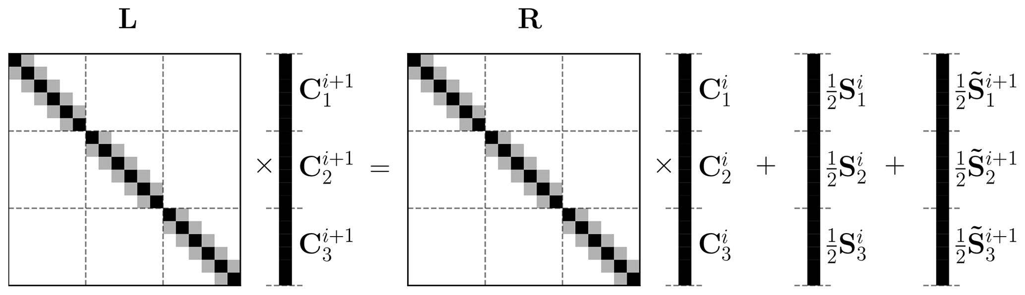
Figure A2 Schematic illustration of Eq. (A11) for a case with N_z=6 spatial cells and N_k=3 classes. The matrices L and R have a block-diagonal structure, where each block is itself tridiagonal. The vectors Cⁱ and Cⁱ⁺¹ are split up into sub-vectors ${\mathit{C}}_{\mathrm{1}},\mathrm{\dots },{\mathit{C}}_{N_k}$, where the elements of C_k are the concentrations of class k in the different spatial cells. Similarly, the reaction term vectors Sⁱ and ${\stackrel{\mathrm{̃}}{\mathbf{S}}}^{i+\mathrm{1}}$ are split into sub-vectors in the same way.

A1.5 Solving for multiple classes

Equation (A1) describes the advection and diffusion of a concentration field C_k(z,t), where the advection velocity w_k represents the rising or settling speed of particles of class k. In this paper, we wish to consider a distribution of particles with different rising or settling speeds, represented by discrete classes.

If there are no reaction terms, there is no interaction between the different classes of particles; hence, the advection–diffusion equation can be solved independently for each class, as described in the previous section. Nevertheless, for reasons of flexibility, it may be convenient to implement an approach where the advection–diffusion equation is solved simultaneously for all classes since this allows interacting reaction terms to be added.

When there are reaction terms that allow the classes to interact, i.e. if the reaction term S_k of class k depends on the concentration of any other class, then we have to solve the advection–diffusion–reaction equation simultaneously for all classes.

Our chosen approach is first to set up the equation system for each individual class. The concentration of class k in the different spatial cells is then represented by a vector C_k, and the matrices in Eq. (A11) for class k we call L_k and R_k. We then create the full matrices L and R as block-diagonal matrices, with the blocks being made up of the matrices ${\mathbf{L}}_{\mathrm{1}},\mathrm{\dots },{\mathbf{L}}_{N_k}$ and ${\mathbf{R}}_{\mathrm{1}},\mathrm{\dots },{\mathbf{R}}_{N_k}$. We next combine the concentrations for all the classes into an overall vector $\mathit{C}=[{\mathit{C}}_{\mathrm{1}},\mathrm{\dots },{\mathit{C}}_{N_k}]$, where N_k is the total number of classes. This leads to a linear system of equations, schematically illustrated in Fig. A2, which can be solved to find the concentrations in all cells for all classes.

As a practical matter, we note that since the matrices L and R are tridiagonal, using a sparse array class in the implementation means that the full matrices do not require any additional memory compared to storing the matrices ${\mathbf{L}}_{\mathrm{1}},\mathrm{\dots },{\mathbf{L}}_{N_k}$ and ${\mathbf{R}}_{\mathrm{1}},\mathrm{\dots },{\mathbf{R}}_{N_k}$ separately.

Appendix B: Distribution of terminal velocities for microplastics

To obtain a distribution of rising and settling velocities for microplastic particles, we combine the distributions for density, size, and shape presented by Kooi and Koelmans (2019) with the empirical relations for terminal velocity obtained by Waldschläger and Schüttrumpf (2019). In the following, we describe the steps leading to a full distribution of rising and settling velocities. The Python code used to obtain the distribution is available on GitHub, both as a script and as a Jupyter Notebook (https://github.com/nordam/Eulerian-and-Lagrangian-methods, last access: 11 September 2023).

We employ a Monte Carlo approach to obtain a velocity distribution, where we draw a sample from each of the distributions describing density, size, and shape, which we can then map to a terminal velocity via the relations of Waldschläger and Schüttrumpf (2019). By repeating this process a large number of times, we obtain a distribution of samples of rising and settling speeds which are consistent with the underlying distributions of density, size, and shape. In the Lagrangian implementation, we can use the sampled velocities directly, while in the Eulerian implementation, we draw a very large number (10⁹) of samples and map them to discrete classes by creating a histogram with the required number of bins.

B1 Density distribution

Kooi and Koelmans (2019) found density to be accurately described by a normal inverse Gaussian distribution, with the parameters μ=0.84, δ=0.097, α=75.1, and β=71.3. Generating random samples from this distribution is straightforward using, for example, the class scipy.stats.norminvgauss from the SciPy library.

B2 Size distribution

The size distribution found by Kooi and Koelmans (2019) is a truncated power-law distribution for the number of particles, where the probability number density for particle size s in micrometres is

$$\begin{array}{}\text{(B1)}& p_N\left(s\right)=P_{\mathrm{0}}{s}^{-\mathit{\alpha }},\end{array}$$

with α=1.6, where s is the size in micrometres and where the range of the distribution is from 20 µm to 5 mm. P₀ is a normalisation factor given by

$$\begin{array}{}\text{(B2)}& P_{\mathrm{0}}={\left(\underset{\mathrm{20}\mathrm{\mu }\mathrm{m}}{\overset{\mathrm{5}\mathrm{mm}}{\int }}{s}^{-\mathrm{1.6}}\mathrm{d}s\right)}^{-\mathrm{1}}\approx \mathrm{3.7573144455}.\end{array}$$

To draw random samples from the distribution with the probability density function (PDF) given by Eq. (B1), we use the inversion method (see e.g. Devroye, 1986, pp. 27–28). We let

$$\begin{array}{}\text{(B3)}& F\left(s\right)=\underset{\mathrm{20}\mathrm{\mu }\mathrm{m}}{\overset{s}{\int }}{p}_N\left(s^{\prime }\right)\mathrm{d}{s}^{\prime }\end{array}$$

be the cumulative distribution function (CDF) of the size distribution. Then, random samples from this distribution can be generated by evaluating F⁻¹(U), where F⁻¹ is the inverse of F(s) (which can be found analytically in this case), and $U\in [\mathrm{0},\mathrm{1}]$ is a uniformly distributed random number.

B3 Shape distribution

Kooi and Koelmans (2019) provide a shape distribution for microplastics in terms of the Corey shape factor (CSF), which is defined as

$$\begin{array}{}\text{(B4)}& \mathrm{CSF}={\displaystyle \frac{H}{\sqrt{LW}}},\end{array}$$

where L, W, and H are respectively the length, width, and height of a particle. We assume that $L\ge W\ge H$ and that the values are scaled by L such that L=1 and $W,H\in [\mathrm{0},\mathrm{1}]$. While Kooi and Koelmans (2019) obtain a single distribution for the CSF in the end, the underlying data are presented as distributions for the width and height for different shape categories, with different relative abundances: fibres (48.5 %), fragments (31 %), beads (6.5 %), films (5.5 %), and foam (3.5 %). Note that these relative abundances only add up to 95 %; hence, we have normalised them by dividing each one by 0.95, and we thus achieve the probabilities listed in Table B1.

For each of the shape categories, the distributions for width and height are assumed to be symmetric, triangular distributions, as described in Kooi and Koelmans (2019), and the distribution parameters for each shape are given in Table S2 of the supplementary materials of Kooi and Koelmans (2019). We also list the distribution parameters in Table B1 for completeness. Generating random samples from a triangular distribution is straightforward with, for example, scipy.stats.triang from the SciPy library.

Table B1 Probability for a microplastic particle to belong to different shape categories, as well as the parameters of the symmetric, triangular distributions for the width and height for each shape category (Kooi and Koelmans, 2019).

Based on the above, our algorithm for the generation of a random CSF for a microplastic particle is as follows:

1. Select a shape category, with the probabilities from Table B1.

2. Generate a random width W and height H by drawing from the triangular distributions for that shape category.

3. Calculate the CSF from Eq. (B4) using the randomly selected W and H, with L=1 by definition.

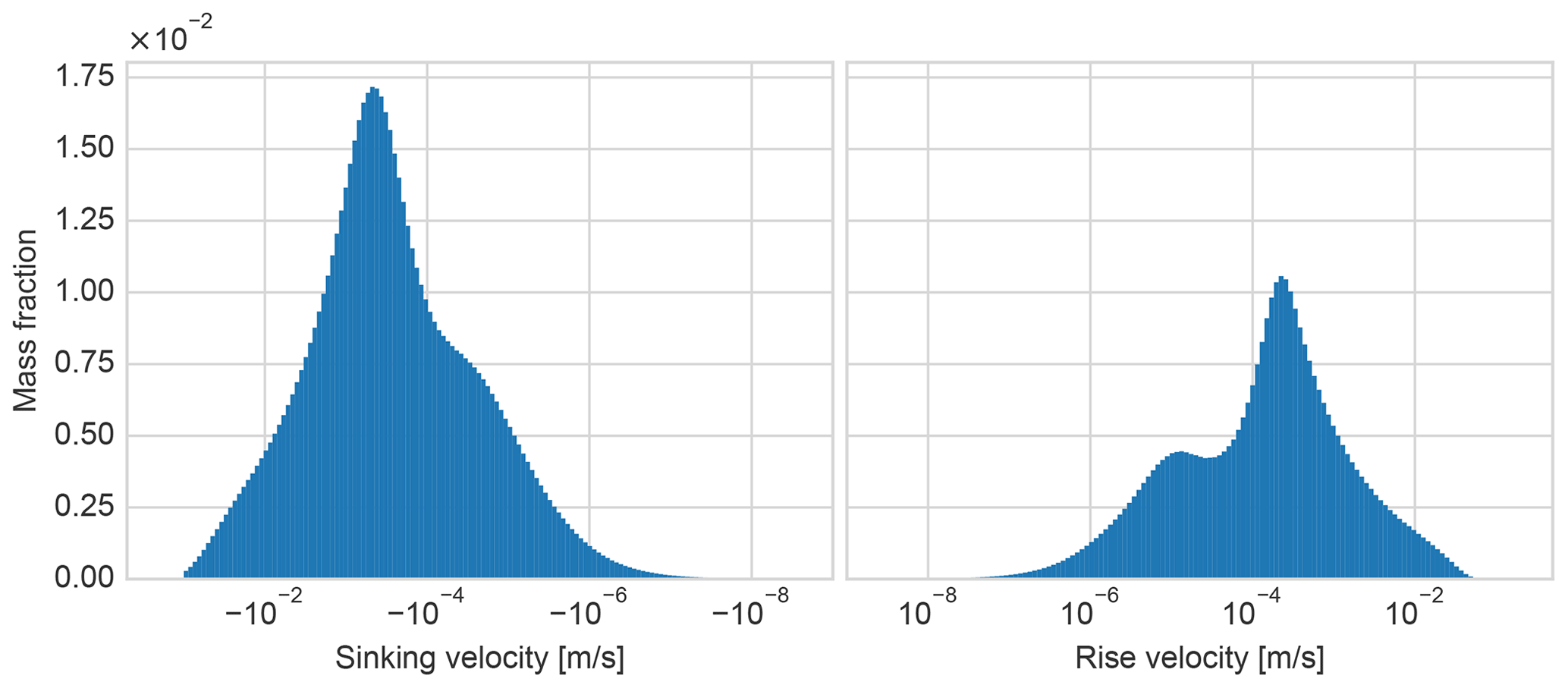
Figure B1 Number distribution of terminal particle velocity, found by mapping 10⁹ velocities onto 128 log-spaced negative bins and 128 log-spaced positive bins, as described in the text.

Table B2 Particle properties used to calculate settling speed. All parameters are generated randomly, except equivalent diameter and shape factors, which are calculated from the random parameters as described. Note that the ranges of width and height depend on length since we assume $L\ge W\ge H$.

B4 Terminal velocities

Waldschläger and Schüttrumpf (2019) provide relations for the rising and settling speeds of microplastic particles in terms of their density, size, and shape. Specifically, they give the terminal velocity as

$$\begin{array}{}\text{(B5)}& v=\sqrt{{\displaystyle \frac{\mathrm{4}}{\mathrm{3}}}{\displaystyle \frac{d_{\mathrm{eq}}}{C_{\mathrm{D}}}}\left|{\displaystyle \frac{{\mathit{\rho }}_s-\mathit{\rho }}{\mathit{\rho }}}\right|g},\end{array}$$

where d_eq is the equivalent diameter (i.e. the diameter of a sphere with the same volume as the particle), ρ_s and ρ are respectively the densities of the particle and the ambient water, g is the acceleration of gravity, and C_D is the drag coefficient.

Four different expressions are given for the drag coefficient, distinguishing between particles that are lighter or denser than water, as well as distinguishing fibres from other shapes (pellets and fragments). For sinking non-fibre particles, the expression is

$$\begin{array}{}\text{(B6)}& C_{\mathrm{D}}={\displaystyle \frac{\mathrm{3}}{\mathrm{CSF}\times \sqrt[\mathrm{3}]{Re}}}.\end{array}$$

For rising non-fibre particles, the expression is

$$\begin{array}{}\text{(B7)}& C_{\mathrm{D}}=\left({\displaystyle \frac{\mathrm{20}}{Re}}+{\displaystyle \frac{\mathrm{10}}{\sqrt{Re}}}+\sqrt{\mathrm{1.195}-\mathrm{CSF}}\right)\times {{\displaystyle \frac{\mathrm{6}}{P}}}^{\mathrm{1}-\mathrm{CSF}}.\end{array}$$

For sinking fibres, the expression is

$$\begin{array}{}\text{(B8)}& C_{\mathrm{D}}={\displaystyle \frac{\mathrm{4.7}}{\sqrt{Re}}}+\sqrt{\mathrm{CSF}}.\end{array}$$

For rising fibres, the expression is

$$\begin{array}{}\text{(B9)}& C_{\mathrm{D}}={\displaystyle \frac{\mathrm{10}}{\sqrt{Re}}}+\sqrt{\mathrm{CSF}}.\end{array}$$

The drag coefficients are given in terms of the CSF, the Reynolds number, and in one case, the Powers' roundness, with the Reynolds number given by

$$\begin{array}{}\text{(B10)}& Re={\displaystyle \frac{v{d}_{\mathrm{eq}}}{\mathit{\nu }}},\end{array}$$

where ν is the kinematic viscosity of the ambient fluid. Given that the drag coefficients depend on the Reynolds number, which in turn depends on the velocity, Eq. (B5) was solved numerically by means of an iterative approach to find the velocity.

The Powers' roundness P is a set of six classes from 1 (very angular) to 6 (well rounded), where particles are assigned a class by comparison with a published photograph of reference particles (Powers, 1953). Powers' roundness is not addressed by Kooi and Koelmans (2019), but Waldschläger and Schüttrumpf (2019, Fig. S6, Supplement) show a histogram of the Powers' roundness distribution. Based on this, we have chosen to use a uniformly distributed random integer between 1 and 6 to represent Powers' roundness. Note that the Powers' roundness only appears in the expression for the drag coefficient for rising pellets and fragments and is thus not used for fibres.

Even though Waldschläger and Schüttrumpf (2019) provide separate drag coefficients for rising and sinking particles, we have chosen to use the same coefficients in both cases. Our reasoning is two-fold: first, from a physical point of view, it is expected that two particles with density ±Δρ relative to water should have terminal velocities with opposite directions but equal magnitude (certainly as long as $\left|\mathrm{\Delta }\mathit{\rho }\right|\ll \mathit{\rho }$). Second, the drag coefficient of sinking non-fibre particles (pellets and fragments) provided by Waldschläger and Schüttrumpf (2019) scales as $R{e}^{-\mathrm{1}/\mathrm{3}}$, while Stokes' law is

$$\begin{array}{}\text{(B11)}& C_{\mathrm{D}}={\displaystyle \frac{\mathrm{24}}{Re}}.\end{array}$$

For small particles, in the lower part of the microplastic size range², the sinking velocities predicted with Eq. (B6) can be 1–2 orders of magnitude higher than those predicted by Stokes' law (even with CSF=1, as would be the case for spherical particles). The drag coefficient provided for rising non-fibre particles, on the other hand, has the same scaling as Stokes' law for small Reynolds numbers. Hence, we have chosen to use this drag coefficient for both rising and sinking particles. In the case of fibres, Eqs. (B9) and (B8) give very similar velocities, but for reasons of symmetry, we have chosen to use Eq. (B9) for both rising and sinking fibres.

B5 Terminal velocity distribution

Based on the description above, we generate random realisations of particle properties, where each particle has the properties shown in Table B2. From these properties, we can calculate terminal velocities using the expressions found by Waldschläger and Schüttrumpf (2019), as described above.

For the Lagrangian implementation, N_p random velocities were generated at the start of each simulation. For the Eulerian implementation, 10⁹ random velocities were generated and mapped to N_k different classes. Given the wide range of velocities, we chose to use equally spaced velocity bins on a log-scale, with positive and negative velocities treated separately. For positive (rising) velocities, we used bins ranging from 10⁻⁸ to 0.1 m s⁻¹, and for the negative velocities, we used bins ranging from −0.3 to $-{\mathrm{10}}^{-\mathrm{8}}$ m s⁻¹. We used the same number of classes to represent the positive and the negative velocities. By always choosing a total number of classes N_k, which is divisible by 2, we get a consistent and automated way to divide the velocity distribution into discrete classes. Note that the approach described here was chosen for simplicity and consistency as our goal is to investigate the numerical convergence with the number of classes.

To get the discrete velocity classes, we generated 10⁹ random velocities and mapped them onto the bins described below, with the velocity of each bin being represented by its midpoint on the logarithmic scale, as described in Sect. 3.1.2. None of the randomly generated velocities were smaller than −0.3 m s⁻¹ or greater than 0.1 m s⁻¹. Approximately 0.02 % of the generated velocities fell between $-{\mathrm{10}}^{-\mathrm{8}}$ and 10⁻⁸ m s⁻¹. These were ignored. The bin counts were then converted to normalised mass fractions, such that the total mass sums to 1. Generating 10⁹ random terminal velocities in this manner took approximately 15 min on a fairly standard PC.

An example histogram showing the distribution of 10⁹ terminal velocities is shown in Fig. B1 using the same 256 bins that were used for the most accurate Eulerian velocity discretisation. Note that this is a number distribution, giving the number of particles with a particular speed. In many cases, a volume (or mass) distribution may be more useful as this would give the volume of microplastics present as particles with a particular speed. However, obtaining a joint volume probability distribution for size and shape from the number distributions presented by Kooi and Koelmans (2019) is outside the scope of this study.

Appendix C: Additional convergence results

Here, we present the convergence of the first moment of the distribution with respect to the time step for the Lagrangian implementation and with respect to the time step and grid cell size for the Eulerian implementation. These results were used to choose suitable numerical parameters for the investigation of convergence with the number of classes and number of particles. They also serve as a sanity check to demonstrate that the numerical schemes behave as expected.

The results are shown in Fig. C1 (case 1), Fig. C2 (case 2), and Fig. C3 (case 3). In each figure, panel (a) shows the convergence of the first moment with the time step in the Lagrangian implementation. For each time step, the first moment was calculated for each value of the time step Δt as the average particle position over 100 simulations, each with 3×10⁶ particles. The error was then found by using the average particle position across 100 simulations with 3×10⁶ particles using a shorter time step of Δt=2 s. The convergence appears to be of the first order, which is as expected for the Euler–Maruyama method as this method has an order of convergence of 1 in the weak sense.

We also note that the error in the first moment of the particle distribution for a Lagrangian stochastic method has two terms: a discretisation term due to the time step and a stochastic term due to the finite number of samples (Pavliotis, 2014, p. 151). The expected magnitude of the stochastic error term can be estimated from the Lindeberg–Lévy theorem, as described in Sect. 2.6. In panel (a) of Figs. C1, C2, and C3, the magnitude of the stochastic sample error is shown as coloured dashed lines, where we have used $N_p=\mathrm{3}\times {\mathrm{10}}^{\mathrm{8}}$ samples, and where the variance of the particle positions for each of the times considered have been assumed to be a good approximation for the (unknown) true variance.

For the Eulerian implementation, the convergence with time step is shown in panel (b) of Figs. C1, C2, and C3, where the number of classes and cells have been kept fixed at N_k=128 and N_z=8000. Finally, the convergence with spatial discretisation for the Eulerian method is shown in panel (c) of Figs. C1, C2, and C3. Here, the time step and number of classes have been kept fixed at Δt=10 s and N_k=128. We observe that convergence is of the second order in both space and time, as expected.

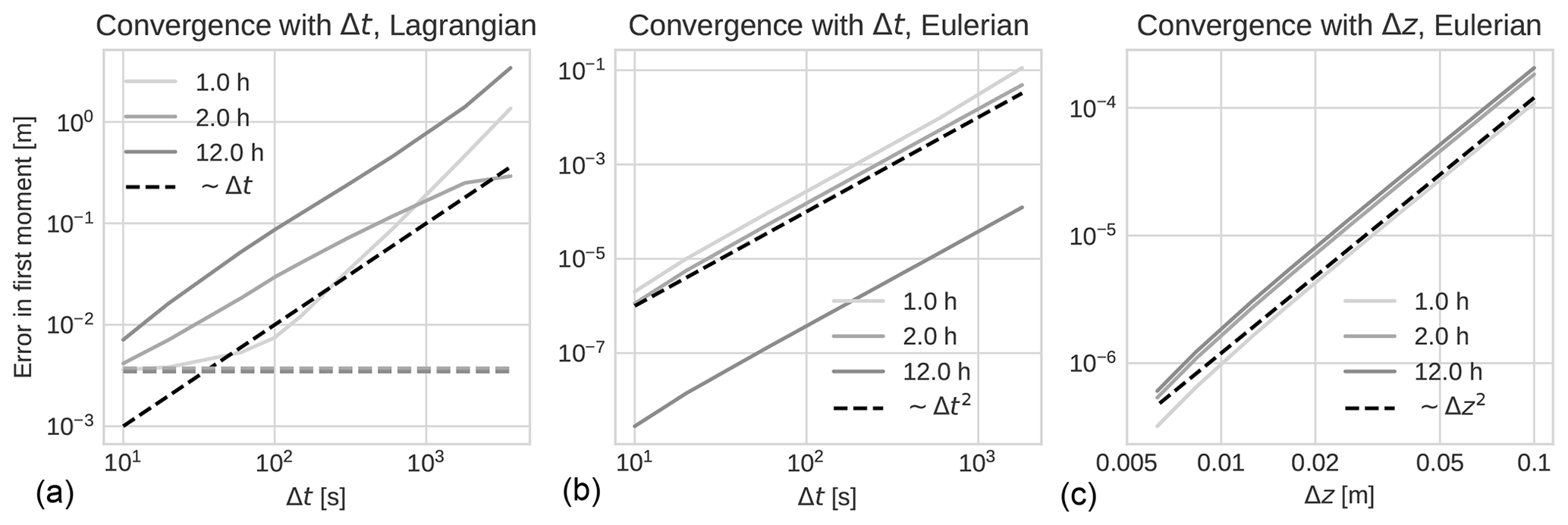
Figure C1 Convergence of the first moment of the distribution in case 1 as a function of the time step for the Lagrangian implementation (a) and as a function of the time step (b) and cell size (c) for the Eulerian implementation. The dashed lines in panel (a) show the level where the sampling error is expected to dominate.

Figure C2 Convergence of the first moment of the distribution in case 2 as a function of the time step for the Lagrangian implementation (a) and as a function of the time step (b) and cell size (c) for the Eulerian implementation. The dashed lines in panel (a) show the level where the sampling error is expected to dominate.

Figure C3 Convergence of the first moment of the distribution in case 3 as a function of the time step for the Lagrangian implementation (a) and as a function of the time step (b) and cell size (c) for the Eulerian implementation. The dashed lines in panel (a) show the level where the sampling error is expected to dominate.