AutoQS v1: automatic parametrization of QuickSampling based on training images analysis

Multiple-point geostatistics are widely used to simulate complex spatial structures based on a training image. The practical applicability of these methods relies on the possibility of finding optimal training images and parametrization of the simulation algorithms. While methods for automatically selecting training images are available, parametrization can be cumbersome. Here, we propose to find an optimal set of parameters using only the training image as input. The difference between this and previous work that used parametrization optimization is that it does not require the definition of an objective function. Our approach is based on the analysis of the errors that occur when filling artificially constructed patterns that have been borrowed from the training image. Its main advantage is to eliminate the risk of overfitting an objective function, which may result in variance underestimation or in verbatim copy of the training image. Since it is not based on optimization, our approach finds a set of acceptable parameters in a predictable manner by using the knowledge and understanding of how the simulation algorithms work. The technique is explored in the context of the recently developed QuickSampling algorithm, but it can be easily adapted to other pixel-based multiple-point statistics algorithms using pattern matching, such as direct sampling or single normal equation simulation (SNESIM).

1 Introduction

Geostatistics is extensively used in natural sciences to map spatial variables such as surface properties (e.g., soils, geomorphology, meteorology) and subsurface geological features (e.g., porosity, hydraulic conductivity, 3D geological facies). Its main applications involve the estimation and simulation of natural phenomena. In this paper, we focus on simulation approaches.

Traditional two-point geostatistical simulations preserve the histogram and variogram inferred from point data (Matheron, 1973). However, inherent limitations make the reproduction of complex structures difficult (Gómez-Hernández and Wen, 1998; Journel and Zhang, 2006). Multiple-point statistics (MPS), by accounting for more complex relations, enables the reproduction of such complex structures (Guardiano and Srivastava, 1993) but comes with its own limitations (Mariethoz and Caers, 2014). The main requirements for using MPS algorithms are (1) analog images (called training images) and (2) appropriate parametrization, while training images can often be provided by expert knowledge, and several methods have been proposed to automatically select one or a subset of appropriate training images among a set of candidates (Pérez et al., 2014; Abdollahifard et al., 2019). However, the parametrization of an MPS algorithm depends not only on the chosen training image but also on the specifics of the algorithm. This makes the task of finding a good parametrization cumbersome, and therefore users often have to resort to trial-and-error approaches (Meerschman et al., 2013). Here we will mainly focus on QuickSampling (QS) (Gravey and Mariethoz, 2020), which has two main parameters: n, which defines the maximum number of conditional data points to consider during the search process, and k, which is the number of best candidates from which to sample the simulated value. Additionally, QS supports a kernel that allows weighting each conditioning pixel in the pattern based on its position related to the simulated pixel. Direct sampling (DS) has the following parameters: n, which has an identical role as in QS; “th”, which represents the pattern acceptance threshold, or the degree of similarity between local data patterns and the training image; and f, which is the maximum proportion of the image that can be explored for each simulated pixel. In summary, n controls the spatial continuity, and k or “th” and f control the variability.

Over the last few years, several studies have addressed the challenge of automatically finding appropriate parameters for MPS simulation. These can be categorized in two approaches. The first approach is to assume that an optimal parametrization is related to the simulation grid (including possible conditioning data), the training image, and the MPS algorithm. In this vein, Dagasan et al. (2018) proposed a method that uses the known hard data from the simulation grid as a reference for computing the Jensen–Shannon divergence between histograms. Following this, they employ a simulated annealing optimization to update the MPS parameters until the metrics achieve the lowest divergence. This method is flexible enough to be adapted to any other metric. The second type of approach assumes that the parametrization is only related to the training image and the MPS algorithm. Along these lines, Baninajar et al. (2019) propose the MPS automatic parameter optimizer (MPS-APO) method based on the cross-validation of the training image (TI) to optimize simulation quality and CPU cost. In this approach, artificially generated gaps in the high-gradient areas of the training image are created, and a MPS algorithm is used to fill those gaps. The performance of a particular parametrization is quantified by assessing the correspondence between the filled and original training data. By design, this approach is extremely interesting for gap-filling problems. The authors state that it can be used for the parametrization of unconditional simulations; however, the use of limited gaps cannot guarantee the reproduction of long-range dependencies. Furthermore, due to the design of the framework for generating gaps, only MPS algorithms able to handle gap-filling problems can be used.

While both approaches yield good results based on their objective functions, they all rely on a stochastic optimization process; therefore, the duration of the optimization process cannot be predetermined or controlled by the user. Furthermore, an objective function is needed, which can be difficult because it depends on the training image used: many metrics can be accounted for in the objective function, such as histogram, variogram, pattern histogram, connectivity function, and Euler characteristic, among others (Boisvert et al., 2010; Renard and Allard, 2013; Tan et al., 2013), or a weighted combination of these. Similarly, one has to define meta-parameters linked to the optimization algorithm itself, such as the cooling rate in simulated annealing or maximum number of iterations. As a result, MPS parameter optimization approaches tend to be complex and difficult to use.

In this contribution, we propose a simplified optimization procedure for simulating complex systems. Rather than using a complex optimization algorithm, our approach focuses on finding optimal parameters to accurately simulate a single pixel in the system. The underlying principle of our approach is that if each pixel is accurately simulated, the resulting sequence of pixels will converge to an accurate representation of the real-world system being simulated. The goal is therefore to find the optimal parameters to simulate a single pixel using the training image as the only reference. Baninajar et al. (2019) showed that computing the prediction error (i.e., the error between the simulation and the reference) is an appropriate metric to identify optimal parameters. To find the optimal parameters for simulating a single pixel, we propose an exhaustive exploration of the parameter space and a computation of the prediction error between the simulation and the reference image.

The remainder of this paper is structured as follows. Section 2 presents the proposed method. Section 3 evaluates the approach in terms of quantitative and qualitative metrics. Finally, Sect. 4 discusses the strengths and weaknesses of the proposed approach and presents the conclusions of this work.

2 Understanding and addressing verbatim copy in multiple-point simulation

The principle underlying multiple-point simulation is that the neighborhood of a given pixel x (the pattern generated by known or previously simulated pixels) is informative enough to constrain the probability density function of the value Z(x). This requires a training image with several pattern repetitions. The extended normal equation simulation (ENESIM) algorithm (Guardiano and Srivastava, 1993) computes the full probability distribution for each simulated pixel. To ensure that enough samples are used, the SNESIM (Strebelle, 2002) and the Impala (Straubhaar et al., 2011) algorithms include a parameter to define a minimum number of pattern replicates. Direct sampling (DS) (Mariethoz et al., 2010) adopts a different strategy by allowing for the interrupted exploration of the training image. It includes a distance threshold parameter that defines what is an acceptable match for a neighborhood; however, too small a threshold typically results in a single acceptable pattern in the training image, leading to exact replication of parts of the training image – a phenomenon known as verbatim copy. To reduce this issue, a parameter f is introduced, controlling the fraction of the explored training image. QuickSampling (QS) (Gravey and Mariethoz, 2020) also suffers from verbatim copy when the number of candidate patterns is set to k=1; the authors recommend the use of k>1 and highlight that k is similar to the number of replicates in SNESIM or IMPALA. A value k=1.5 in QS can be seen as SNESIM with a minimum number of replicates of 1 for 50 % of the simulated values and 2 for the remaining values.

The definition of verbatim copy is the unintended pasting of a large section from the training image to the simulation (patch-based approaches do so intentionally, e.g., Rezaee et al., 2013). This means that the relative position of the simulated values is the same as that in the training image. This occurs when the neighborhood constraints on the simulated pixels are too strong, and only the exact same patterns as those in the training image are acceptable. To detect this issue, a common strategy is to create a position map (similar to the index map), which represents the provenance of simulated values by mapping their original coordinates in the training image, as shown in Fig. 1.

Figure 1 illustrates the most common forms of verbatim copy. The pure verbatim (the most common type of verbatim copy) is a simple copy of a large part of the image, with all pixels in the same order inside of the patches. Block verbatim typically appears when there are many replicates of a very specific type of pattern in the training image and few replicates of all other patterns. Consequently, the MPS algorithm uses common patterns for transitioning between copied blocks resulting from rare patterns. Structural verbatim occurs when the copied portion spreads throughout the simulation without giving a direct impression of copying (e.g., pure verbatim over a subset of pixels). Structural verbatim tends to appear when large-scale structures are unique in the training image, which often allows a visually satisfying image to be quickly obtained, but with large non-stationary features identical to the training image. Often, users are willing to allow verbatim on large-scale structures, but this can easily introduce bias between simulations. This is one of the hardest types of verbatim to detect. Typically, this can occur when the maximum neighborhood radius is too large, leading to the duplication of large structures in the initial phase of the simulation. Finally, no verbatim, which is the expected result of simulations, occurs when the position of pixels does not have any particular structure (i.e., their position is unpredictable).

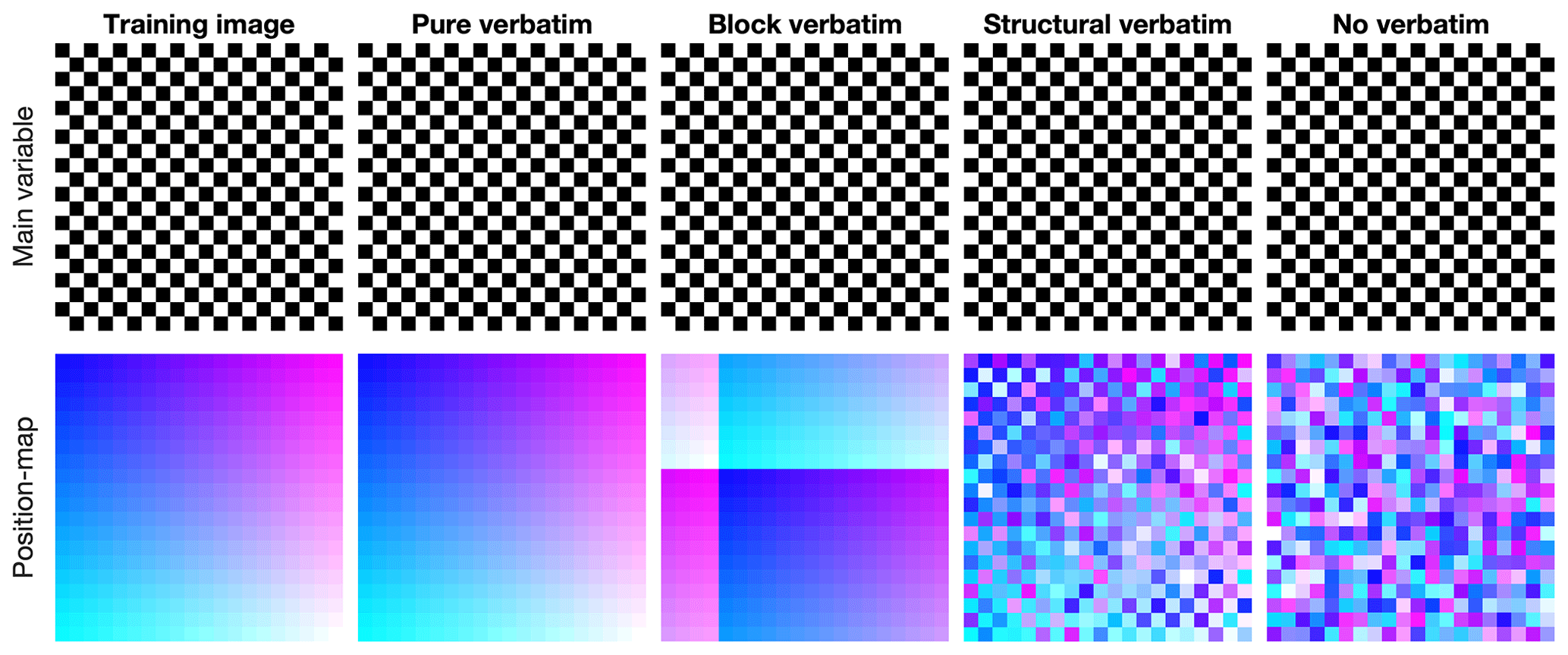
Figure 1 Visualization of verbatim copies using a position map. This is an extreme case that highlights that verbatim is not defined by the values simulated but by their position in the training image.

3 Method

The objective of the approach presented here is to find an optimal set of parameters using only the training image and knowledge of the simulation algorithm's mechanics. The simulation algorithm is not used in this context; in fact, simulations are not required to obtain a proper calibration with the proposed method. The main target application of the presented approach is the pattern-matching simulation algorithm QuickSampling (QS), where the values, at a pixel scale, are directly sampled from the training image. The method is suitable for the simulation of continuous and/or categorical variables.

Simulation algorithms such as QS can be summarized by Algorithm 1. The key operation occurs at Line 3, which is when the algorithm searches for an optimal match based on the neighboring conditioning data.

Algorithm 1 The sequential simulation algorithm. n, k, and ω, the parametrization for QS.

Inputs:

T: training images

S: simulation grid, including the conditioning data

P: simulation path

θ: parametrization

n: number of neighbors

k: the number of best candidates

ω: the kernel, by default uniform

1:

for each unsimulated pixel x following the path P: do

2:

Find the neighborhood N(x) in S composed of the n(θ) closest neighbors

3:

Find a candidate in T those matches N(x) using the parametrization θ

4:

Assign the value of the selected candidate to x in S

5:

end for

Here, we propose a divide-and-conquer approach that splits any pixel-based sequential simulation into its atomic operation: the simulation of a single pixel. We assume that if all pixels are perfectly simulated, then the resulting simulation should also be good. By a perfectly simulated pixel, we mean a pixel that respects the conditional probability distribution. When simulating a pixel, there may be numerous potential valid values, but at the very least, there should be one valid value; i.e., the conditional probability distribution should be represented in the data. This can be formalized by the following condition:

$$\begin{array}{}\text{(1)}& \left|\left\{A\mathrm{|}P\left(A\mathrm{|}N\left(x\right)\right)>\mathrm{0}\right\}\right|\ge \mathrm{1},\end{array}$$

where |.| represents the cardinality of a set. P(A|N(x)) denotes the probability of A (a given value) knowing N(x), the neighborhood.

The proposed approach consists of finding a set of parameters that results in accurate samples for each pattern. At the same time, we want to avoid systematically sampling perfect matches (the exact same neighborhood is available in the training image), which results in verbatim copy.

The search for the optimal parametrization is carried out by exhaustive exploration (Algorithm 2), and the choice of optimal parameters is based on a prediction error defined as the difference between the original value of the pattern and the value of the selected pattern in the training image.

Algorithm 2 The AutoQS algorithm.

Inputs:

D: list of stages of the simulation (i.e., pattern decimation levels, equivalent to fractions of the simulation path)

θ: list of discretized parameters

T the training images

V a set of random positions (in practice we generated the random position on the fly)

1:

for each possible combination of D and θ do for all v∈V:

2:

Sample a neighborhood N(v) from T and decimate it according to stage D

3:

Using θ, find a candidate in T that matches N(v) excluding for v itself

4:

Compute the error ε between the selected candidate and Z(v)

5:

end for

6:

Analyze the errors ε to determine the best θ for each D

The proposed algorithm explores a discretized parameter space θ (Algorithm 2, Line 1) (e.g., for QS: nkω). While this discretization is natural for some parameters, such as n that is an integer, it can require an explicit discretization for other parameters, such as the kernel in QS (or “th” in DS). Furthermore, a key component of our method is the exploration of the parameter space for several representative stages D of the simulation (Algorithm 2, Line 1). In the case of a random path, the progress of the simulation is directly related to the density of the neighborhoods; i.e., when x % of the pixels are simulated, on average x % of neighbors are informed. To reproduce this behavior, at each stage D, we randomly decimate patterns extracted from the TI by keeping only x % pixels informed. For each combination D and θ, multiple measures over a set of random locations V ($\mathrm{500}<\left|V\right|<\mathrm{10}\mathrm{000})$ are computed in Lines 1–5 in Algorithm 2, with their mathematical expression shown in Eq. (2):

$$\begin{array}{}\text{(2)}& \begin{array}{rl}& \mathit{\epsilon }\left(\mathit{\theta },D,T\right)=\\ & \sqrt{{\displaystyle \frac{\mathrm{1}}{\left|V\right|}}\sum _{v\in V}{\left(Z\left(v\right)-Z\left(\underset{T\setminus \mathit{\left\{}v\mathit{\right\}}}{\mathrm{Cand}}\left(\mathit{\theta },N\left(v,D\right)\right)\right)\right)}^{\mathrm{2}}},\end{array}\end{array}$$

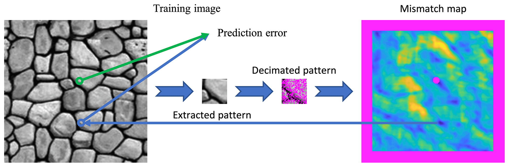
where Cand(θ,N) returns a single candidate position for a given neighborhood N and follows the parametrization θ. N(v,D) denotes a neighborhood around v that is decimated according to stage D. V represents a random set of positions in the training image, and Z(v) refers to the actual value at position v∈V in the training image. To avoid parameters that generate verbatim copy of the training image, the position v and its direct neighbors (in a small radius (here 5 pixels)) are excluded from the set of potential candidates. The set of candidates considering this exclusion is denoted by T∖{v} in Eq. (2). Furthermore, in the case of equality between several optimal options, we set as a rule to take the cheapest parameter set in terms of computational cost (e.g., the smallest n). Figure 2 graphically represents the entire algorithm. Finally, for each stage considered, the set of parameters with the minimum associated error ε is considered optimal (Algorithm 2, Line 6):

$$\begin{array}{}\text{(3)}& \mathit{\epsilon }\left({\mathit{\theta }}_{\mathrm{optimal}},D,T\right)=\underset{\mathit{\theta }}{min}\mathit{\epsilon }\left(\mathit{\theta },D,T\right).\end{array}$$

Figure 2 All steps for a single pattern, summarizing Algorithm 2, Lines 2–4.

4 An efficient implementation

In practice, the implementation of Algorithm 2 separates θ into two parameter subsets: θ_h and θ_s. The θ_h subset consists of all parameters that influence the calculation of a single pattern match, which varies depending on the algorithm used. For instance, in QS, it includes the number of neighbors n and the kernel ω, while in DS, it comprises the threshold “th” and n. On the other hand, θ_s encompasses parameters related to the sampling process of the training image. For QS, this includes the number of candidates to keep k, while for DS, it involves the fraction f of the training image being scanned.

Our implementation precomputes and stores all matches for a specific θ_h parametrization (e.g., a value of n and all matches for k). Consequently, the saved matches of θ_h can be employed to swiftly evaluate all options for the parameters in $\mathit{\theta }={\mathit{\theta }}_{\mathrm{h}}\times {\mathit{\theta }}_{\mathrm{s}}$ (e.g., we can process for $k=\mathrm{1},\mathrm{2},\mathrm{3},\mathrm{\dots }{k}_{\max }$). This two-phase approach considerably decreases redundant calculations.

The algorithm can be further accelerated by terminating the estimation of ε if the error remains at a high level after assessing only a small amount of samples from V (here set to 500). To this end, we increase V for the parameter combinations of interest, i.e., parametrization with potentially the lowest ε. This entails iterating and verifying at each step whether additional computations are required. Only places respecting the following inequality are refined with extra measures:

$$\begin{array}{}\text{(4)}& \mathit{\epsilon }\left(\mathit{\theta },D,T\right)-\mathit{\epsilon }\left({\mathit{\theta }}_{\min },D,T\right)<{\displaystyle \frac{\mathrm{1}}{\mathrm{2}}}\mathit{\sigma }\left(\mathit{\theta },D,T\right)+{\displaystyle \frac{\mathrm{1}}{\mathrm{2}}}\mathit{\sigma }\left({\mathit{\theta }}_{\min },D,T\right),\end{array}$$

with

$$\begin{array}{c}{\displaystyle }\mathit{\epsilon }\left({\mathit{\theta }}_{\min },D,T\right)=\underset{\mathit{\theta }}{min}\mathit{\epsilon }\left(\mathit{\theta },D,T\right)\\ {\displaystyle }\begin{array}{rl}& \mathit{\sigma }\left(\mathit{\theta },D,T\right)=\\ & \sqrt{{\displaystyle \frac{\mathrm{1}}{\left|V\right|}}\sum _{v\in V}{\left(\left(Z\left(v\right)-Z\left(\underset{T\setminus \mathit{\left\{}v\mathit{\right\}}}{\mathrm{Cand}}\left(\mathit{\theta },N\left(v,D\right)\right)\right)\right)-\mathit{\epsilon }\left(\mathit{\theta },D,T\right)\right)}^{\mathrm{2}}}\end{array},\end{array}$$

where ε(.) represents the error and σ(.) represents the standard deviation of all differences, between estimated and true values.

5 Results

5.1 Optimization of two parameters

All experimental tests in this section are performed using the training image shown in Fig. 2, and the stages D are distributed following a logarithmic scale.

As a first test, we use the configuration θ_h={n} and θ_s={k}. The kernel ω is defined as uniform, meaning that it has a constant value and is not part of the optimization. The outcome is represented in Fig. 3, with the optimal number of candidates k and number of neighbors n as a function of the density D, which is assimilated to the progression during the simulation. The ignorance threshold is defined as the average error between elements of the marginal distribution. It represents the error value at which no further information can be derived from the neighborhood, meaning that the simulated values can equivalently be drawn from the marginal distribution.

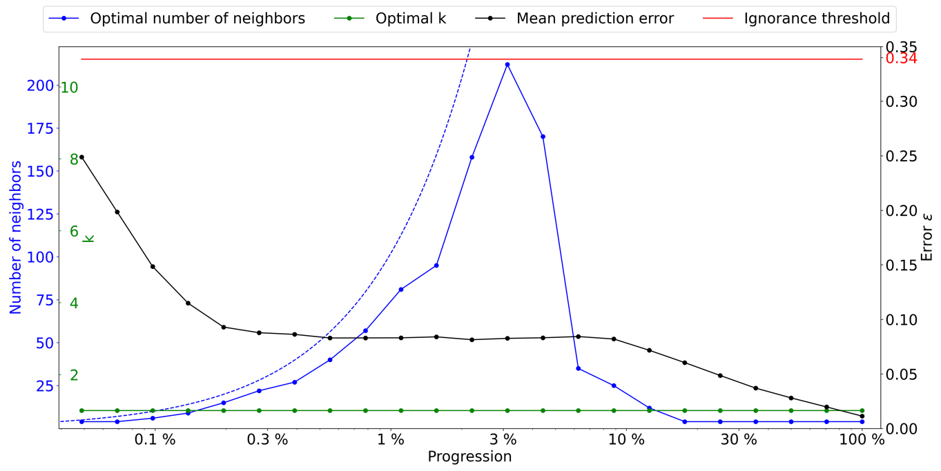
Figure 3 Optimal parameters for QS (k in green and number of neighbors in blue) as a function of the progression, with the associated prediction error (in black). The red line represents the ignorance threshold. The dashed blue line indicates the average maximal number of neighbors.

The optimal k remains small (in fact 1) throughout the simulation, which is probably due to the limited size of the training image in this case. It seems important to use many neighbors in the early stages of the simulation. The number of neighbors increases until approximately 3 % of the simulation. This is followed by a subsequent drastic reduction, indicating that once the large structures are informed, only the few direct neighbors are important. It seems logical that MPS algorithms simulate large structure first and then smaller patterns in a hierarchical manner where each smaller structure is part of the larger one. We, however, note that it remains generally difficult to predict the optimal settings as a function of the simulation stage. This indicates that the use of a single parametrization for the entire MPS simulation is generally suboptimal, and the parameters should be adapted as the simulation progresses.

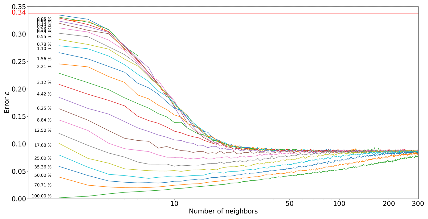
Figure 4 Pattern error as a function of the number of neighbors n, with k=1, where each curve represents a neighborhood density D.

Figure 4 shows the evolution of ε as a function of the number of neighbors n and the simulation progression D. Two regimes are visible: in the first percentages of the simulation, each extra neighbor is informative and improves simulation quality. However, as the neighborhoods become denser, the importance of spatial continuity takes over, and only the few neighbors are really informative. This two-step process is expected, as random large-scale features are generated first, and then the image is filled with consistent fine-scale structures. Furthermore, it shows that using a large number of neighbors at the end of the simulation generates suboptimal results, which could explain the small-scale noise that is sometimes visible in some MPS simulations.

5.2 Optimization of three parameters

Here, we use the following configuration ${\mathit{\theta }}_{\mathrm{h}}=\left\{n,\mathit{\alpha }\right\}$ and θ_s={k}, and we consider kernels as having a radial exponential shape, i.e., ${\mathit{\omega }}_i=e^{-\mathit{\alpha }.d_i}$. The weight of a given position i in the kernel ω is defined as ω_i and its distance to the kernel center as d_i.

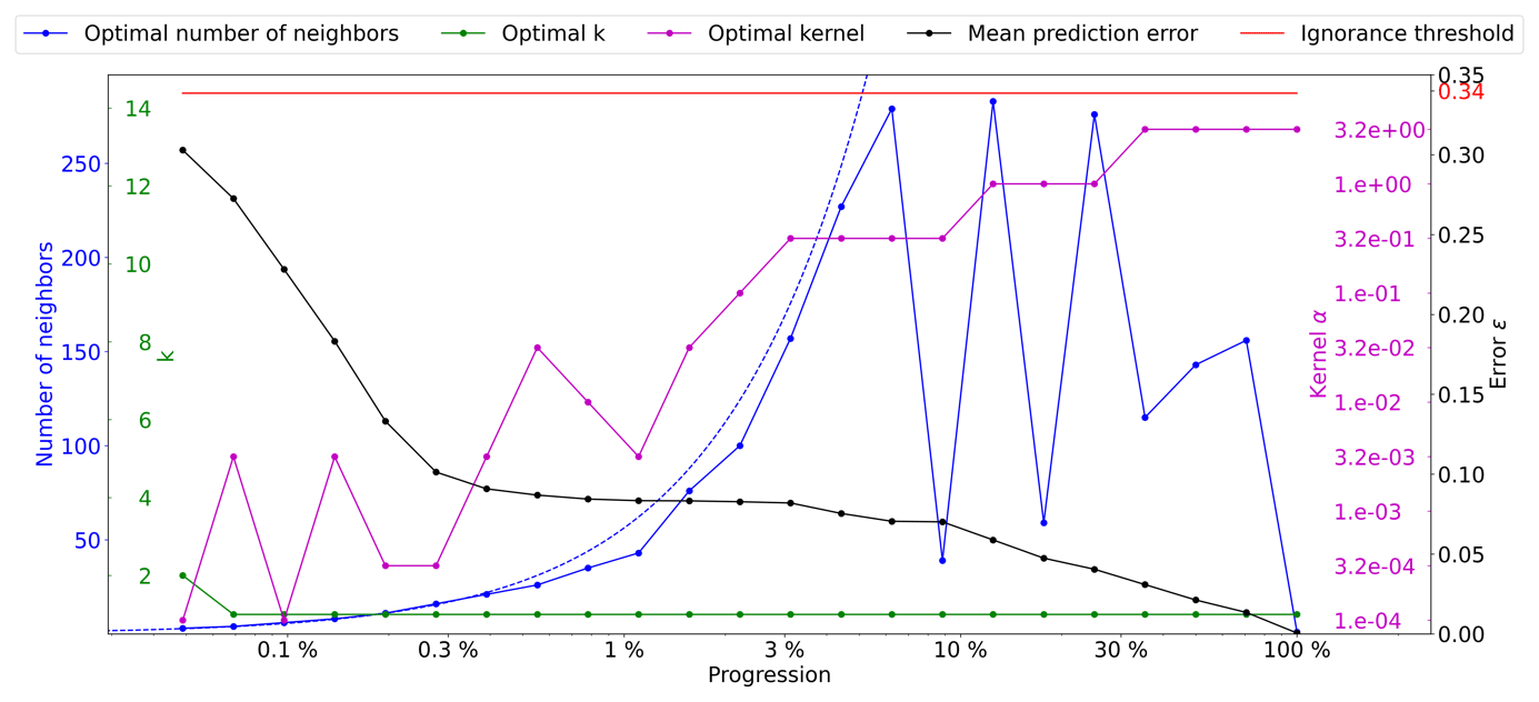
Figure 5 Optimal parameters for QS (k in green, number of neighbors in blue, and best kernel in magenta), as a function of the simulation progress, with the associated prediction error (in black). The dashed blue line indicates the average density for the neighborhood considered. The ignorance threshold in red.

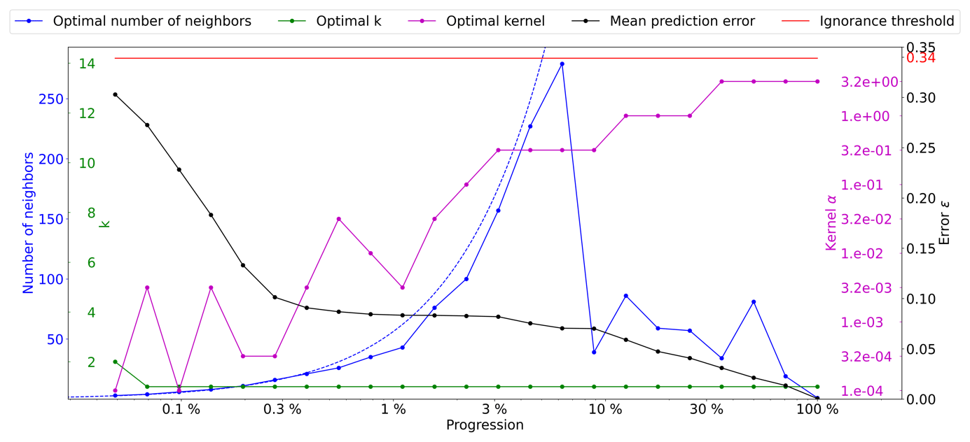
Figure 6 Optimal parameters for QS (k in green, number of neighbors in blue, and the best kernel in magenta) as a function of the progression, with the associated prediction error (in black). The dashed blue line is the average density for the neighborhood considered. The ignorance threshold is in red.

The results presented in Fig. 5 demonstrate the impact of the number of neighbors and narrow kernels (characterized by high α values) on the evolution of the QS parameters. Specifically, it can be observed that interactions arise between these two factors, resulting in slightly erratic calibrated parameters. As the number of neighbors increases, the weights assigned to the furthest neighbors become negligible with larger α values. This means that these far-away neighbors, despite being considered, have very little influence. This insensitivity only occurs for large n values, leading to minimal differences between possible configurations and noise in the metric.

As expressed in the methodology section, in cases of a similar error, the cheapest solution is considered. In the case of QS, having a large number of neighbors can marginally increase the computational time; therefore, we introduce a small tolerance that results in favoring small n values. It is formulated as a small cost for each extra neighbor, i.e., by adding $\mathrm{5}\times {\mathrm{10}}^{-\mathrm{5}}\times \left(max\left(T\right)-min\left(T\right)\right)$ for each extra neighbor. However, the speed-up during simulation was limited to up to 10 %. Figure 6 shows a quality similar (ε curves) to that in Fig. 5 but with the added tolerance. As expected, the number of neighbors required during the simulation drastically decreases as advanced simulation stages and the fluctuations in n are avoided.

5.3 Sequential simulation using automatic calibration

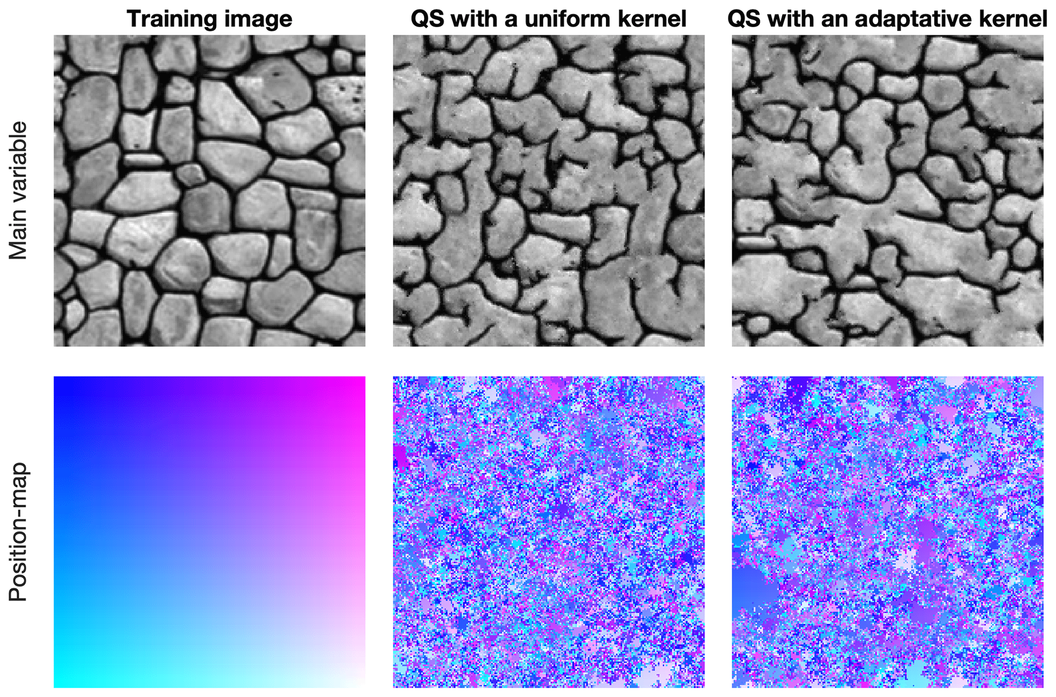
Figure 7 shows qualitative results using the evolutive parametrization resulting from the proposed autocalibration, using a case study that was published in Gravey and Mariethoz (2020). QS with an adaptive kernel refers to the use of different values of α for the kernel as a function of the simulation progression. In this case, the results are similar to state-of-the-art simulations using a manual calibration. Tests using QS with a uniform kernel fail to reproduce some structures; in particular, the size of the objects is incorrect. Each position map shows few homogenous areas; therefore, realizations are produced with a low rate of verbatim copy.

Figure 7 Simulation using QS with parameters generated by the automatic calibration.

From a quantitative evaluation, Fig. 8 illustrates different metrics (variograms, connectivity as a structural indicator, and the Euler characteristic as noise indicator) (Renard and Allard, 2013) across a set of 100 realizations. The automatic calibration method proposed here allows obtaining better-quality simulations than in Gravey and Mariethoz (2020).

Figure 8 shows that variogram and connectivity metrics are well reproduced, although they have not been directly constrained in the calibration process. Indeed, the parameter optimization only considers the simulation of single pixels and never computes global metrics over an entire grid.

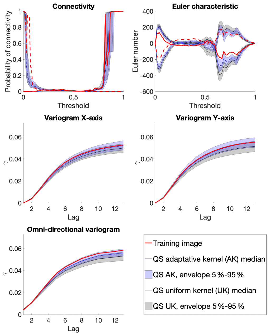
Figure 8 Benchmark between QS with an adaptive kernel (Fig. 6) and a uniform (without) kernel (Fig. 3) over 100 simulations for five different metrics.

6 Discussion and conclusion

The proposed method allows for the automatic calibration of QS and potentially similar pixel-based MPS approaches, reaching a quality similar to or better than that of manual parametrization from both quantitative and qualitative points of view. Furthermore, it demonstrates that the optimal parametrization should not remain constant and instead needs to evolve with the simulation progression. The metrics confirm the good reproduction of training patterns, and the method finds a calibration that avoids verbatim copy. One major advantage of our approach is the absence of a complex objective function, which often itself requires calibration.

A limitation of our approach is that it cannot be used to determine an optimal simulation path because it focuses on the simulation of a single pixel. It also does not optimize the computational cost required for a simulation.

The computation time necessary to identify the appropriate parameters is contingent upon the expected quality. However, the maximum time required for completion is predictable and depends on the number of patterns tested. If required, the calibration can be further refined based on prior outcomes without restarting the entire process; this can be achieved by adjusting D, incorporating additional kernels, or increasing |V|. In certain instances, adjusting the kernel parameter offers only minor improvements while necessitating a substantial number of computations. Employing a more streamlined parameter space can yield comparable calibration and significantly reduce the computational cost. This streamlined parameter space can be established, for instance, by subsampling the number of neighbors according to a squared function (2, 4, 9, 16, 25, etc.) or by leveraging external or expert knowledge.

The proposed methodology was evaluated in multivariate scenarios, resulting in a more expansive parameter space compared to single-variable cases. Although the approach yields satisfactory parameters, the inclusion of extra parameters significantly extends the computation time, rendering the process impractical, particularly when dealing with four or more variables.

In the context of testing the generality of our approach, calibration was computed on multiple training images (found in the Appendix). The calibration pattern with two regimes (n large, then n small) seems to be universal, at least for univariate simulations. While the position of the abrupt transition between regimes seems to vary greatly (between 0.5 % and 20 % of the path), the overall shape remains the same. Therefore, the approach proposed by Baninajar et al. (2019), in which long ranges are not considered, could be extended by using large n values in the early stages of the simulation. While we show that it is possible to calibrate a parametric kernel, in future work one can envision the optimization of a nonparametric kernel where the weight of each individual neighbor w_i is considered a variable to optimize using ε as an objective function (e.g., using a machine learning regression framework).

The study of the evolution of parameters shows a smooth behavior of the average error. Therefore, the use of multivariate fitting approaches to estimate the error surface with fewer evaluations could be an interesting solution to speed up the parametrization. The use of machine learning to take advantage of transfer learning between training images also has a high potential.

Appendix A

This appendix contains a similar calibration for other training images.

A1 Stone

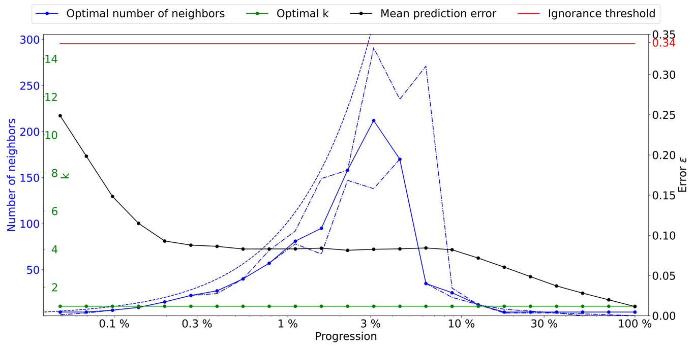
Figure A1 Optimal parameters for QS (k in green and number of neighbors in blue) as a function of the progression, with the associated prediction error (in red). The red line represents the ignorance threshold. The dashed blue line is the average density for the neighborhood considered. The dot-dashed line represents the variability in 1 % of the error.

A2 Strebelle

This section studies the application of the proposed method using the Strebelle training image (Strebelle, 2002).

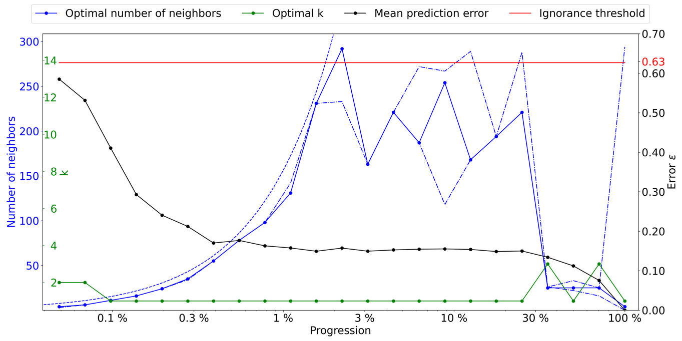
Figure A2 Optimal parameters for QS (k in green and number of neighbors in blue) as a function of the progression, with the associated prediction error (in red). The red line represents the ignorance threshold. The dashed blue line is the average density for the neighborhood considered. The dot-dashed line represents the variability in 1 % of the error.

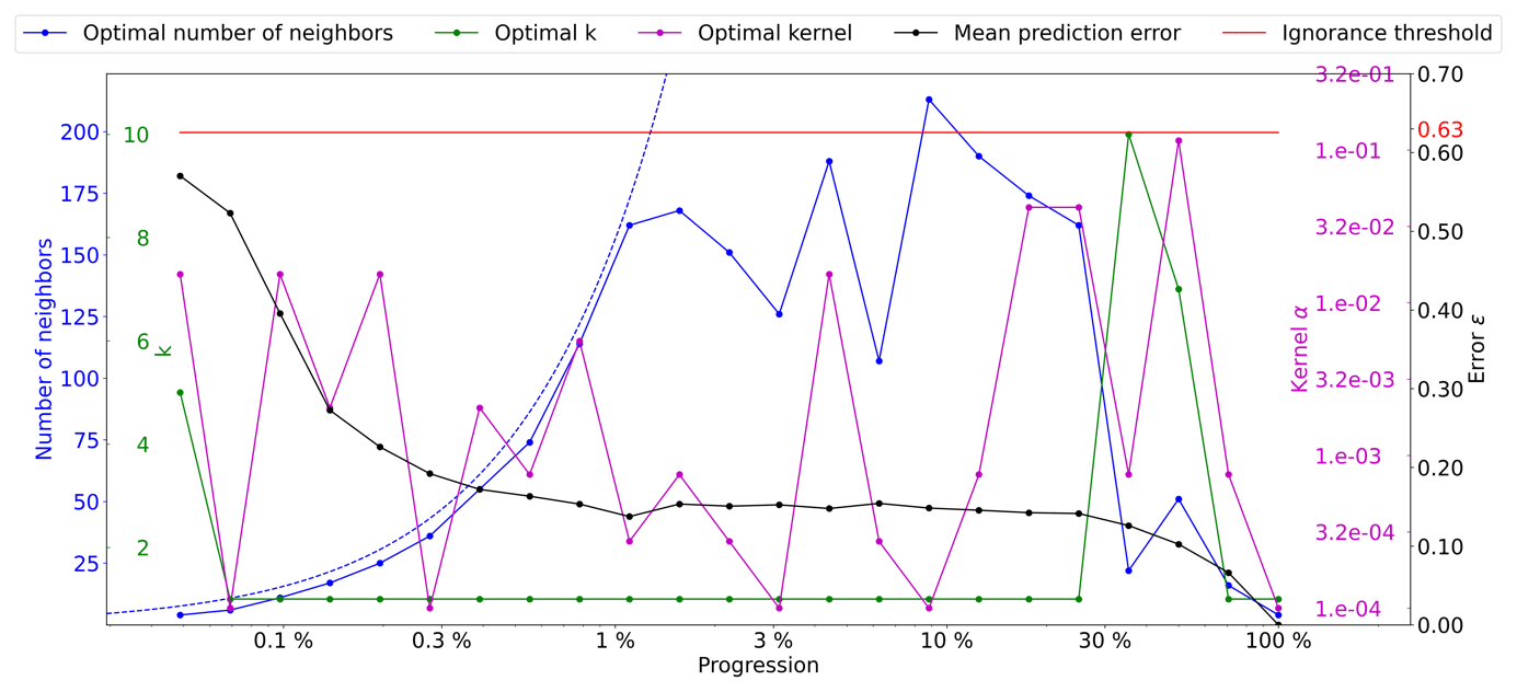
Figure A3 Optimal parameters for QS (k in green, number of neighbors in blue, and the best kernel in magenta) as a function of the progression, with the associated prediction error (in red). The dashed blue line is the average density for the neighborhood considered.

Figure A4 Simulation using QS using parameters generated by the automatic calibration.

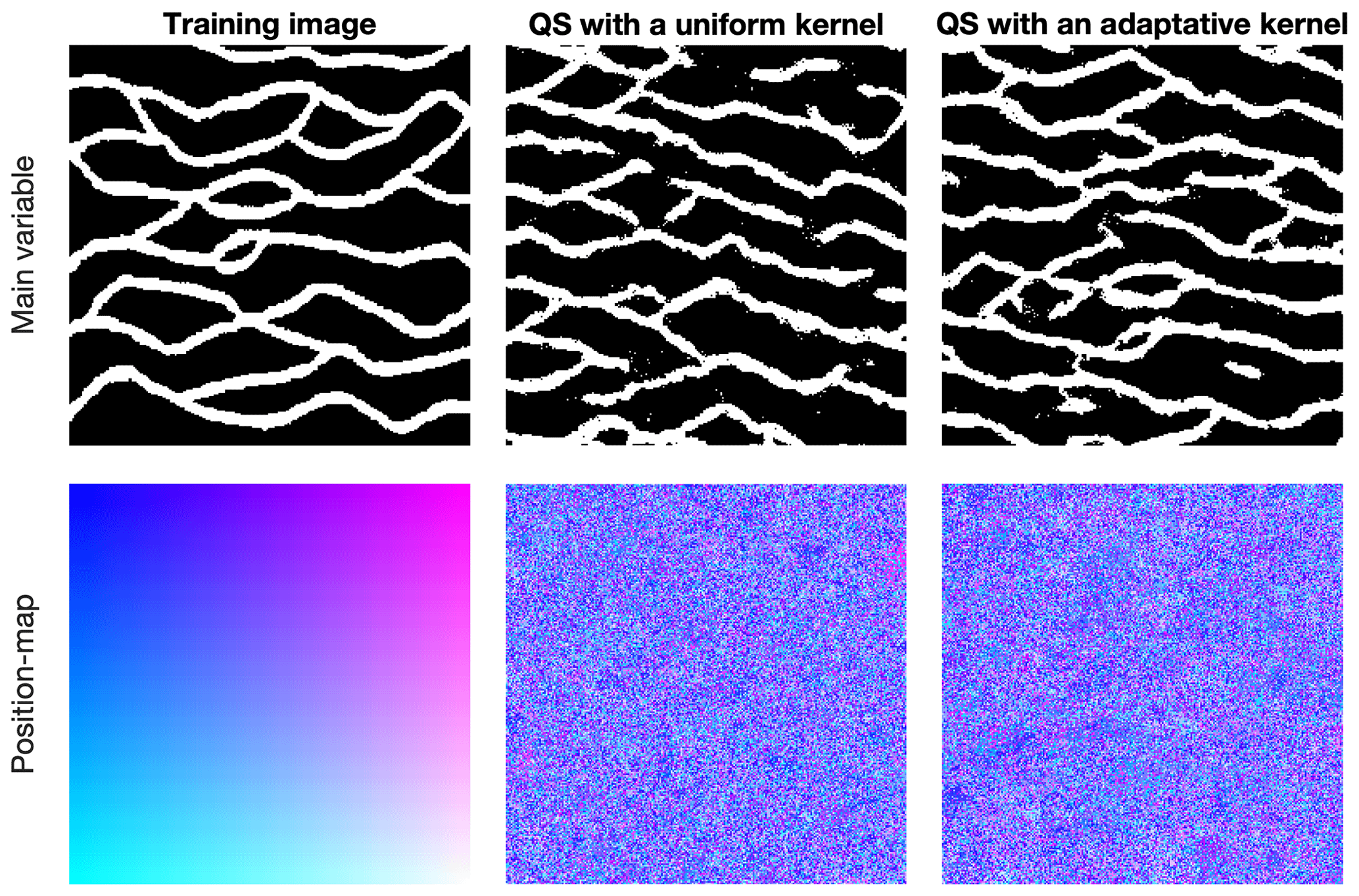
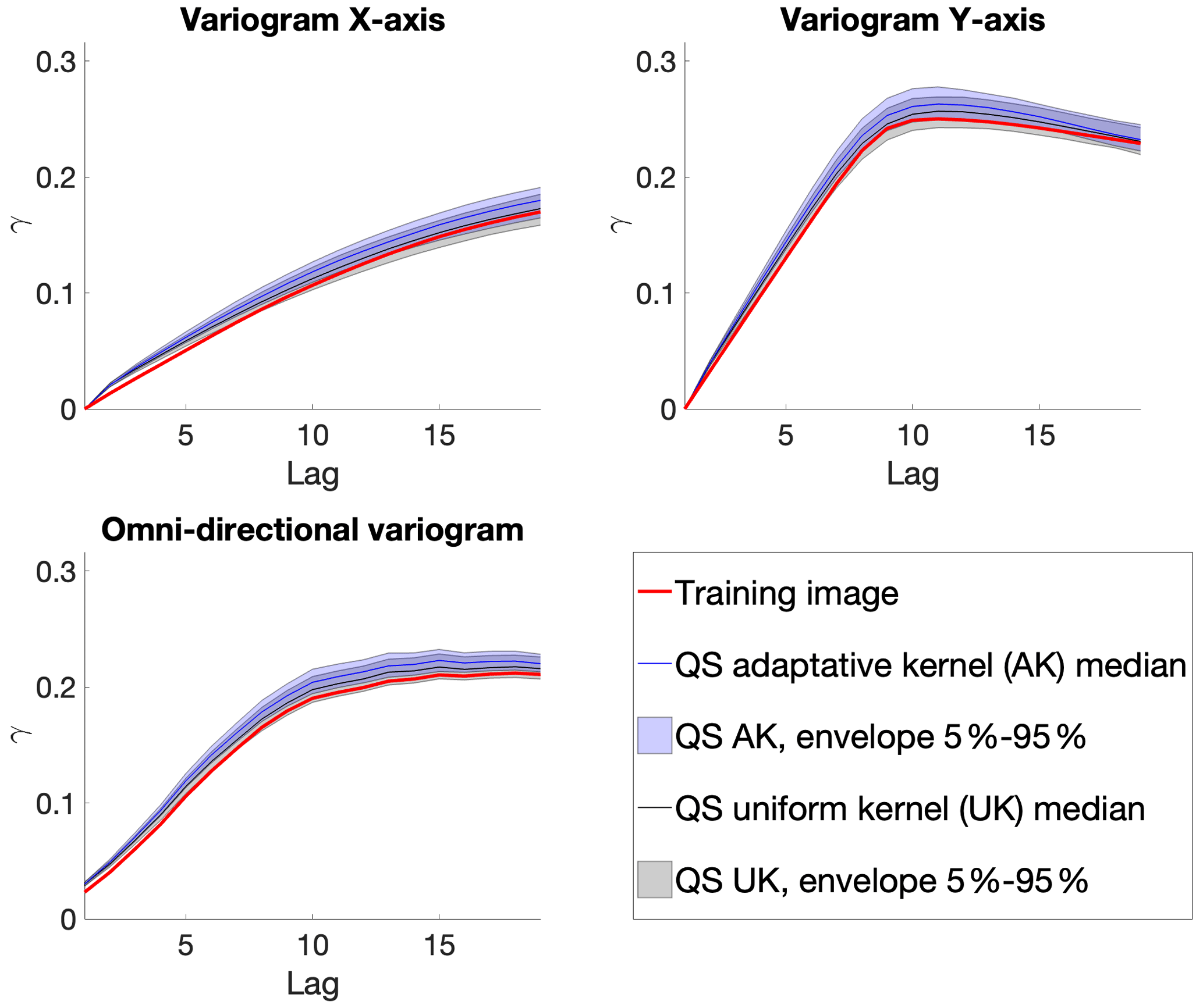
Figure A5 Benchmark between QS with adaptive kernel (Fig. A3) and uniform (without) kernel (Fig. A2) over 100 simulations for five different metrics.

A3 Lena river delta

This section studies the application of the proposed method using the Lena river delta training image (Mahmud et al., 2014).

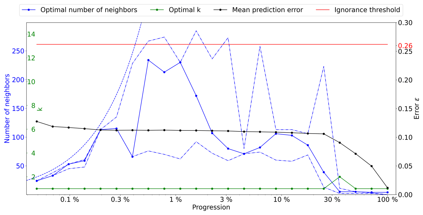
Figure A6 Optimal parameters for QS (k in green and number of neighbors in blue) as a function of the progression, with the associated prediction error (in red). The red line represents the ignorance threshold. The dashed blue line is the average density for the neighborhood considered. The dot-dashed line represents the variability in 1 % of the error.

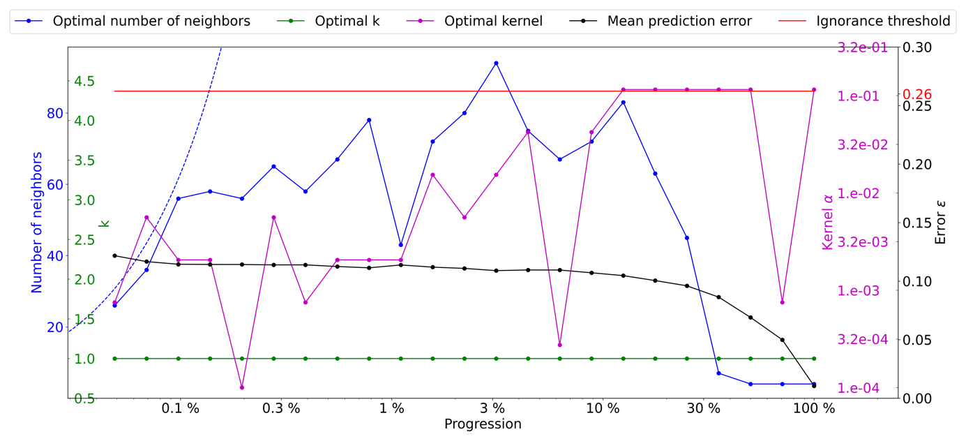
Figure A7 Optimal parameters for QS (k in green, number of neighbors in blue, and the best kernel in magenta) as a function of the progression, with the associated prediction error (in red). The dashed blue line is the average density for the neighborhood considered.

Figure A8 Simulation using QS and using parameters generated by the automatic calibration.

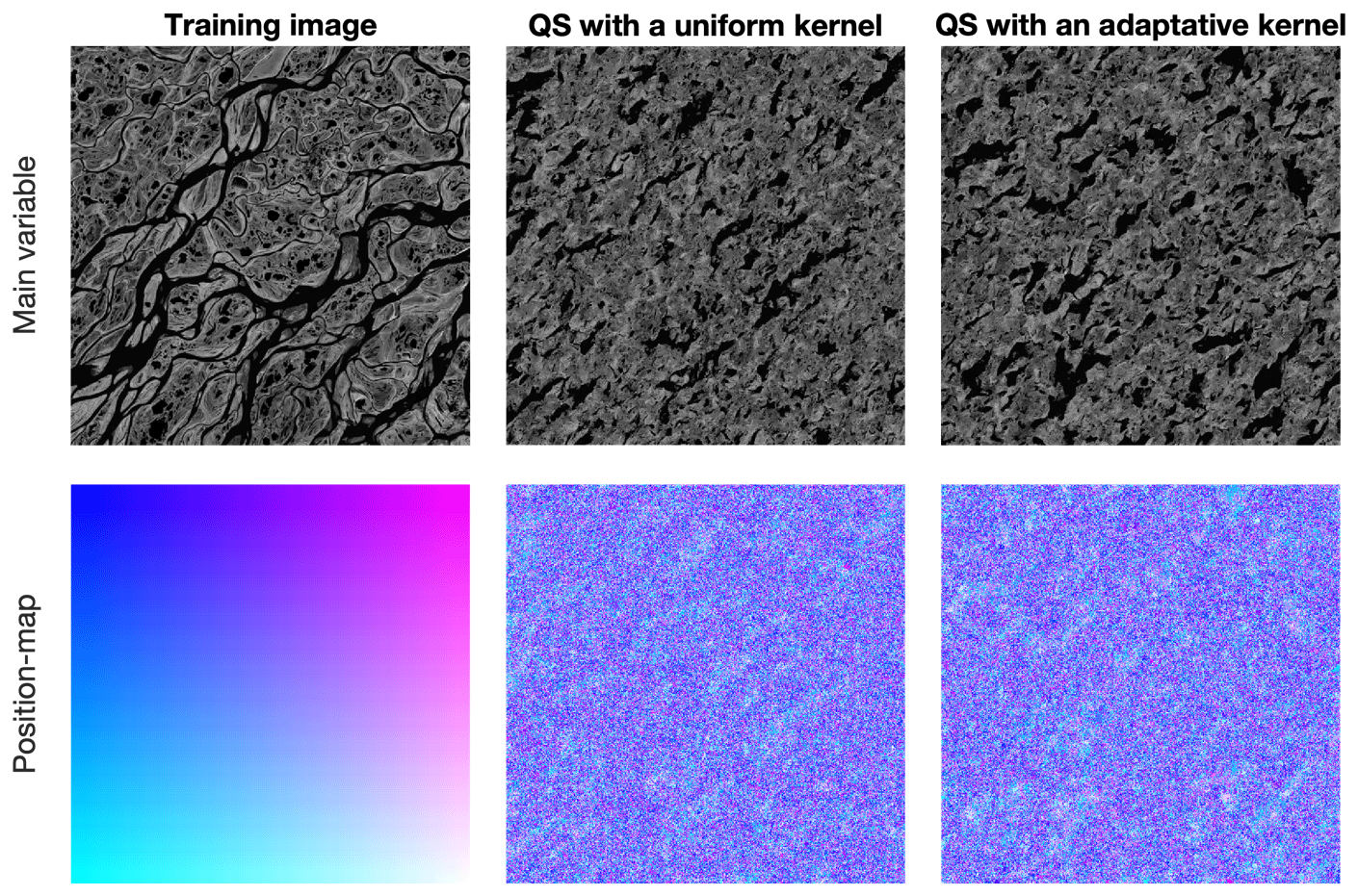
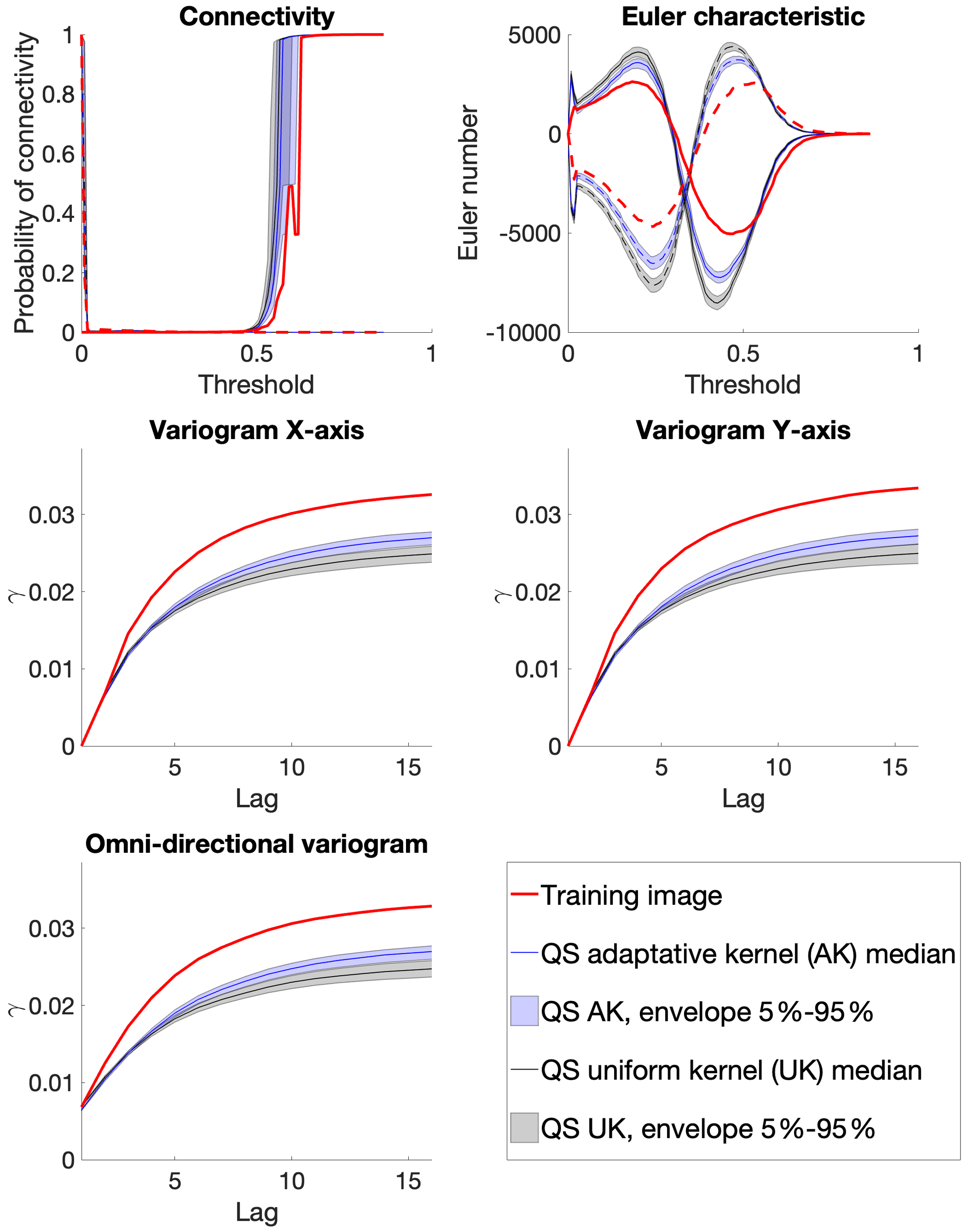
Figure A9 Benchmark between QS with adaptive kernel (Fig. A7) and uniform (without) kernel (Fig. A6) over 100 simulations for five different metrics.