Simulation model of Reactive Nitrogen Species in an Urban Atmosphere using a Deep Neural Network: RNDv1.0

Nitrous acid (HONO) plays an important role in the formation of ozone and fine aerosols in the urban atmosphere. In this study, a new simulation approach is presented to calculate the HONO mixing ratios using a deep neural technique based on measured variables. The Reactive Nitrogen Species using a Deep Neural Network (RND) simulation is implemented in Python. The first version of RND (RNDv1.0) is trained, validated, and tested with HONO measurement data obtained in Seoul, South Korea, from 2016 to 2021. RNDv1.0 is constructed using k-fold cross validation and evaluated with index of agreement, correlation coefficient, root mean squared error, and mean absolute error. The results show that RNDv1.0 adequately represents the main characteristics of the measured HONO, and it is thus proposed as a supplementary model for calculating the HONO mixing ratio in a polluted urban environment.

1 Introduction

Surface ozone (O₃) pollution has worsened over continental areas (Arnell et al., 2019; Monks et al., 2015; IPCC, 2014; Varotsos et al., 2013). Particularly, a warmer climate is expected to increase the surface O₃ concentrations and peak levels in polluted regions depending on its precursor levels (IPCC, 2023). As a short-lived climate pollutant (SLCP), O₃ interacts with the global temperature via positive feedback (Myhre et al., 2017; Shindell et al., 2013; Stevenson et al., 2013). Therefore, accurate predictions of the mixing ratios and variations in the surface O₃ are essential. While operational models such as the Community Multiscale Air Quality (CMAQ) model have been widely used for this purpose, uncertainties still arise from poorly understood chemical mechanisms involving reactive nitrogen oxides (NO_y) and volatile organic compounds (VOCs), as well as the lack of their measurements (Cheng et al., 2022; Akimoto et al., 2019; Shareef et al., 2019; Canty et al., 2015; Mallet and Sportisse, 2006)

In the urban atmosphere, NO_y typically includes NO_x (NO + NO₂), HONO, HNO₃, organic nitrates (e.g., PAN), NO₃, N₂O₃, and particulate NO${}_{\mathrm{3}}^{-}$. These species are produced and recycled through photochemical reactions until they are removed through wet or dry deposition (Li et al., 2020; Wang et al., 2020; Liebmann et al., 2018; Brown et al., 2017). NO_y plays an important role in critical environmental issues concerning the Earth's atmosphere from local air pollution to global climate change (Ge et al., 2019; Sun et al., 2011). The oxidation of NO to NO₂ and finally to HNO₃ is the backbone of the chemical mechanism producing ozone (O₃) and PM_2.5 (particulate matter with size ≤2.5 µm), and it determines the oxidization capacity of the atmosphere. Recently, as O₃ has still increased even with decreasing NO_x emissions over many regions, including East Asia, interest in the heterogeneous reaction of NO_y, which is yet to be understood, has increased (Stadtler et al., 2018; Brown et al., 2017). Currently, the lack of measurements of individual NO_y species is hindering a comprehensive understanding of the heterogeneous reactions (Akimoto and Tanimoto, 2021; Y. Chen et al., 2018; Stadtler et al., 2018; X. Wang et al., 2017; Anderson et al., 2014).

In particular, the evidence for the heterogeneous formation of HONO in relation to high PM_2.5 and O₃ occurrences in urban areas is increasing (e.g., Y. Li et al., 2021). As an OH reservoir, HONO expedites the photochemical reactions involving VOCs and NO_x in the early morning, leading to O₃ and fine aerosol formation. Nonetheless, its formation mechanism has not been elucidated sufficiently enough to be constrained in conventional photochemical models. In addition to the reaction of NO with OH (Bloss et al., 2021), various pathways of HONO formation have been suggested via laboratory experiments, field measurements, and model simulations: direct emissions from vehicles (S. Li et al., 2021) and soil (Bao et al., 2022); photolysis of particulate nitrate (Gen et al., 2022); and heterogeneous conversion of NO₂ on various aerosol surfaces (Jia et al., 2020), the ground surface (Meng et al., 2022), and microlayers of the sea surface (Gu et al., 2022). Among these, the heterogeneous reaction mechanism on the surface is of major interest.

HONO has been mostly measured during intensive campaigns in urban areas using various techniques and instruments, such as a long path absorption photometer (Xue et al., 2019; Kleffmann et al., 2006), chemical ionization mass spectrometry (Levy et al., 2014; Roberts et al., 2010), ion chromatography (Gil et al., 2020; Xu et al., 2019; Ye et al., 2016; Vandenboer et al., 2014), a monitor for aerosols and gases in ambient air (MARGA) (Xu et al., 2019), and quantum cascade and tunable infrared laser differential absorption spectrometry (QC-TILDAS) (Gil et al., 2021; Lee et al., 2011). Among these methods, QC-TILDAS has served as a reference for the intercomparison of measurement data obtained using different techniques due to its high time resolution and stability (Pinto et al., 2014). Previous studies have reported that the maximum HONO with levels of several parts per billion (ppb) has been observed at nighttime. In comparison, the WRF-Chem and RACM2 models captured approximately 67 %–90 % of the observed HONO in megacities such as Beijing (Liu et al., 2019; Tie et al., 2013).

In recent years, machine learning (ML) methods have been employed in the atmospheric science field for pattern classification (e.g., new particle formation event), forecasting, and spatiotemporal modeling of O₃ and PM_2.5 (Arcomano et al., 2021; Cui and Wang, 2021; Kang et al., 2021; Krishnamurthy et al., 2021; Shahriar et al., 2020; G. Chen et al., 2018; Joutsensaari et al., 2018). Among the ML methods, the neural network (NN) architecture is widely used owing to its powerful ability to process large volumes of data. In particular, a multilayer artificial NN (ANN), referred to as a deep NN (DNN), employs statistical methods to learn nonlinear relationships within the data and yield optimal solutions for a target species without prior knowledge of the underlying physicochemical processes (Schultz et al., 2021; Reichstein et al., 2019). DNN is more beneficial than other NN architectures, such as convolution NN or long short-term memory, because it works well for discrete spatiotemporal data. Generally, the performance of a DNN is similar to or better than that of other ML methods for small and large datasets (Baek and Jung, 2021; Dang et al., 2021; Sumathi and Pugalendhi, 2021).

The DNN method requires lots of data to employ it for atmospheric chemical constituent estimation; therefore, the size of the measurement data is a limiting factor for trace species, such as HONO, that are not routinely measured. In this regard, previous studies have attempted to estimate the daily average HONO mixing ratio by employing ensemble ML models with satellite measurements (Cui and Wang, 2021). Furthermore, a simple NN architecture using ground measurement variables that are believed to be deeply involved in HONO formation was used to calculate the hourly HONO mixing ratio (Gil et al., 2021). The accuracy of the hourly HONO estimated from input variables, such as aerosol surface areas and mixed layer height, is rated better than the daily HONO estimate.

This study aims to develop a user-friendly Reactive Nitrogen Species using a DNN (RNDv1.0) simulation model that estimates the HONO mixing ratios from the real-time measurements of criteria pollutants and meteorological variables. This study is the first to calculate the HONO mixing ratios using RNDv1.0. The entire construction process is comprehensively described, and the performance is evaluated via comparison with the results of simulations using a commonly used model and observations over several years.

2 Model description

The RNDv1.0 development follows systematic steps that are similar to a general ML model construction workflow, including data collection, preprocessing data, building the DNN, training and validating the model, and testing the model performance (Fig. 1). RNDv1.0 is written in Python, and the libraries necessary to build and operate RNDv1.0 are listed in Table 1. The dataset used to train, test, and validate the model can be downloaded from Gil (2021).

Figure 1 The main processes for configuring RNDv1.0 (^* signifies calculated values).

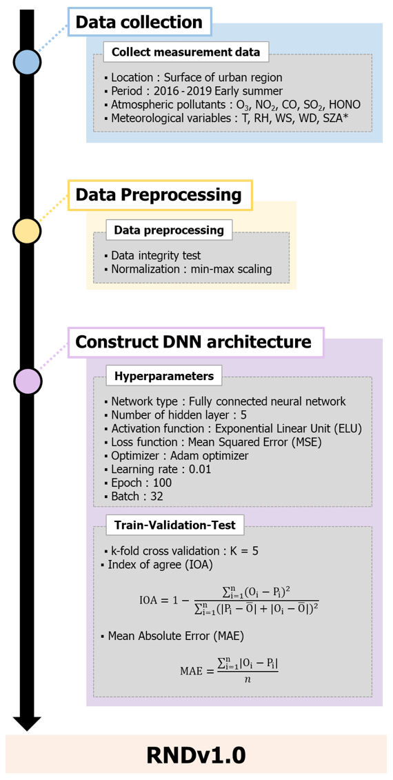
Table 1 Resources for constructing the RND model.

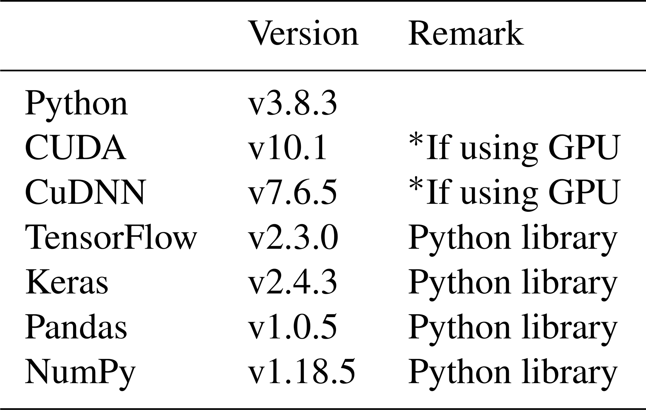
^* GPU signifies graphic processing unit.

2.1 Collection of measurement data for model construction

To construct RNDv1.0, measurement data were obtained, including HONO, reactive gases, and meteorological variables. Note that the HONO measurement data were used for model construction but are not required to run the RND model. The HONO mixing ratio was measured in Seoul, South Korea, using a QC-TILDAS system during May–June 2016, June 2018, and April–June 2019 (Gil et al., 2021), as well as a MARGA system during May–June 2021 and October–November 2021 (Gil et al., 2023). When testing and evaluating the atmospheric HONO measurement methods, QC-TILDAS was chosen as the reference method to compare the ambient HONO mixing ratios measured using several different techniques owing to its advantages of having low detection limits (∼ 0.1 ppbv) and high temporal resolution (Pinto et al., 2014). More details on measurements can be found elsewhere (Gil et al., 2021).

HONO was measured at the Olympic Park (37.52^∘ N, 127.12^∘ E) during the Korea–United States Air Quality (KORUS-AQ) study in 2016 (Kim et al., 2020; Gil et al., 2021), at the campus of Korea University (37.59^∘ N, 127.03^∘ E) in 2018 and 2021 (Gil et al., 2023), and at another site near the Korea University campus (37.59^∘ N, 127.08^∘ E) in 2019 (NIER, 2020) (Fig. S1). In addition to HONO, trace gases including O₃, NO₂, CO, and SO₂, as well as meteorological variables including temperature (T), relative humidity (RH), wind speed (WS), and wind direction (WD), were measured. Note that HONO was not significantly correlated with any of these variables (Fig. S2). The measurement statistics for the entire experimental periods are presented in Tables 2 and S1. In brief, the 10th and 90th percentile mixing ratios of hourly HONO, NO₂, and O₃ were 0.3 and 2.0 ppbv, 10.0 and 47.0 ppbv, and 8.0 and 75.0 ppbv, respectively.

Table 2 Input variables and their concentrations (10th–90th percentile of the hourly measurements), coverage, and scale factors for the RNDv1.0 model. Measurements were conducted in Seoul during May–June in 2016 and 2019.

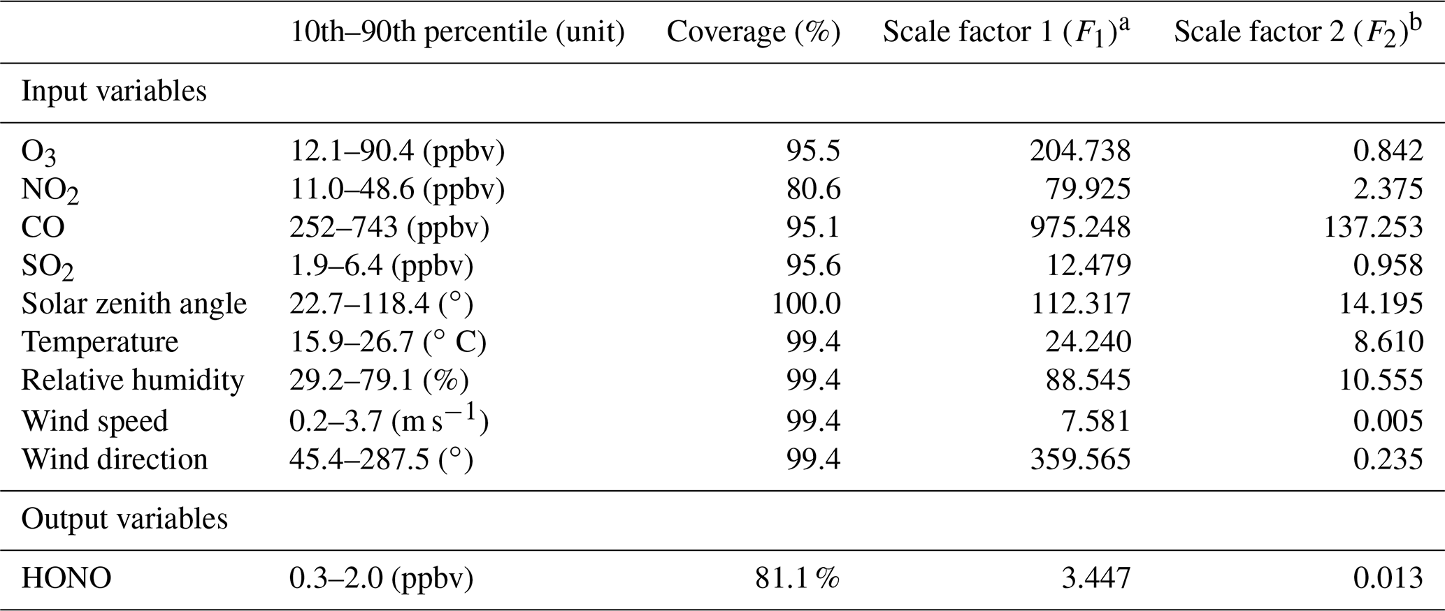
^a Maximum–minimum. ^b Minimum value.

2.2 Data preprocessing

The observation dataset was prepared for RNDv1.0 model construction. As input variables, hourly measurements of chemical and meteorological variables were used, including the mixing ratios of O₃, NO₂, CO, and SO₂, along with T, RH, WS, WD, and solar zenith angle (SZA), to estimate the target species, HONO, as the output. The WD in degrees was converted to a cosine value for continuity. In the last step of data processing, hourly measurement sets were removed from the input dataset if any of the nine variables was missing. Finally, 54.2 % of all the available measurement data (2847 data points) were used to construct and evaluate RNDv1.0.

Since the measurements of the nine variables considered varied over a wide range of different units, they were normalized to avoid bias during the calculations. Among the widely used normalization methods, the “min–max scaling” method was adopted, and the input variables were normalized against the minimum and maximum values herein (Eq. 1):

$$\begin{array}{}\text{(1)}& x_{\mathrm{sca}}={\displaystyle \frac{x_{\mathrm{raw}}-F_{\mathrm{2}}\left(X\right)}{F_{\mathrm{1}}\left(X\right)}},\end{array}$$

where x_raw is the raw data, x_sca is the scaled value, and the scale factors of F₁ and F₂ correspond to the maximum–minimum and minimum values of the input variable (X), respectively, which are listed in Table 2.

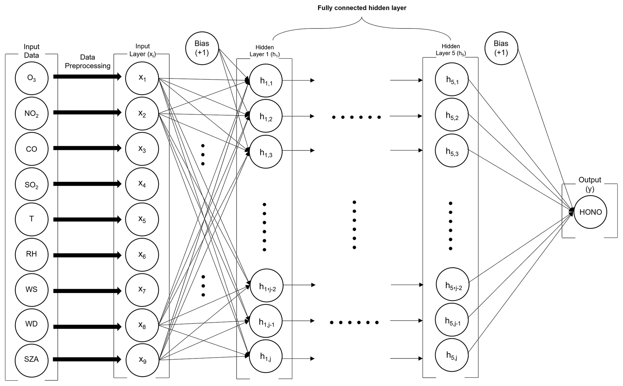
2.3 Neural network architecture and hyperparameters

The network was built using the above input variables to calculate HONO. RNDv1.0 comprises five hidden layers (Fig. 2), which employ an exponential linear unit (ELU) as an activation function (Eq. 2).

$$\begin{array}{}\text{(2)}& \mathrm{ELU}:\mathit{\varphi }\left(x\right)=\left\{\begin{array}{l}{e}^x-\mathrm{1}(x<\mathrm{0})\\ x(x\ge \mathrm{0})\end{array}\right.\end{array}$$

In a DNN, an activation function creates a nonlinear relationship between an input variable and an output variable. When constructing a DNN model, ELU offers the advantage of a fast training process and exhibits better performance in handling negative values than other activation functions (Ding et al., 2018; T. Wang et al., 2017). Moreover, the mean squared error and Adam optimizer were applied as the loss function and optimization function, respectively. The learning rate, epoch, and batch were set as 0.01, 100, and 32, respectively.

Figure 2 Structure of the deep neural network built for RNDv1.0.

2.4 Model training and k-fold cross validation

RNDv1.0 was trained, validated, and tested with the HONO measurements obtained during May–June 2016 and June 2018, April–June 2019, and May–June 2021 and October–November 2021, respectively (Fig. 3). The number of data used for the training and validation was 1122, and that for testing was 1725.

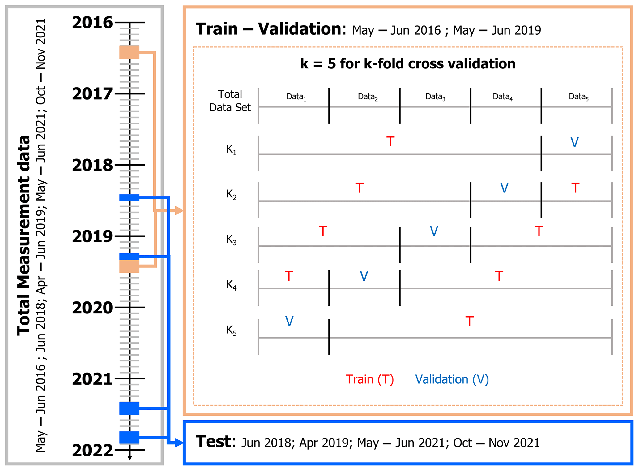
Figure 3 Training, validation, and test design to build RNDv1.0 using the measurement data. The k-fold cross validation was performed using five randomly divided subsets of the training dataset.

Using the hyperparameters specified in the previous section, the model performance was first validated using the k-fold cross validation (KFCV) method, which is especially useful for small datasets (Bengio and Grandvalet, 2003). In the KFCV method (Fig. 3), the entire data are randomly divided into k subsets, of which k−1 sets are used for training and the remaining one is used for validation. In this study, k was set to 5. The accuracy was determined via the index of agreement (IOA), which is expressed as follows (Eq. 3):

$$\begin{array}{}\text{(3)}& \mathrm{IOA}=\mathrm{1}-{\displaystyle \frac{{\sum }_{i=\mathrm{1}}^n(O_i-P_i{)}^{\mathrm{2}}}{{\sum }_{i=\mathrm{1}}^n(\left|P_i-\stackrel{\mathrm{‾}}{O}\right|+\left|O_i-\stackrel{\mathrm{‾}}{O}\right|{)}^{\mathrm{2}}}},\end{array}$$

where O_i, P_i, $\stackrel{\mathrm{‾}}{O}$, and n are the observed value, predicted value, average of the observed values, and number of nodes, respectively.

As IOA varies according to the number of nodes, it was calculated for the measured (HONO_obs) and calculated (HONO_mod) mixing ratios by varying the number of nodes from 0 to 100 in each hidden layer. The best performance was obtained with 41 nodes, for which the average IOA was 0.89 ± 0.01 (Fig. 4). The high IOA value signifies that the performance of RNDv1.0 is adequate, and it is capable of simulating the ambient HONO mixing ratio using the routinely measured criteria pollutants and meteorological variables.

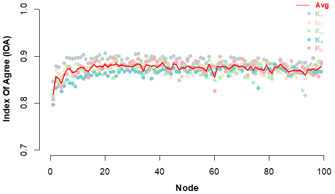
Figure 4 Index of agreement (IOA) for k-fold cross validation. Solid circle and red line represent IOA for each validation (k=5) and the average of five validation sets at each node number.

The performance of RNDv1.0 was compared with that of other models, including CMAQv5.3.1 (Appel et al., 2021), random forest (RF), and single-layer ANN (Gil et al., 2021), using the 2016 measurement data. The RF model was constructed using the KFCV method and the same input variables as RNDv1.0 (Fig. S4). Its performance was evaluated based on mean absolute error (MAE), root mean square deviation (RMSE), and Pearson correlation coefficient (r):

$$\begin{array}{}\text{(4)}& {\displaystyle }\mathrm{MAE}={\displaystyle \frac{{\sum }_{i=\mathrm{1}}^n\left|O_i-P_i\right|}{n}},\text{(5)}& {\displaystyle }\mathrm{RMSE}=\sqrt[\mathrm{2}]{{\displaystyle \frac{{\sum }_{i=\mathrm{1}}^{\mathrm{n}}(O_i-P_i{)}^{\mathrm{2}}}{n}}},\text{(6)}& {\displaystyle }r={\displaystyle \frac{\mathrm{cov}(O,P)}{{\mathit{\sigma }}_O{\mathit{\sigma }}_P}},\end{array}$$

where σ and cov denote the standard deviation and covariance, respectively.

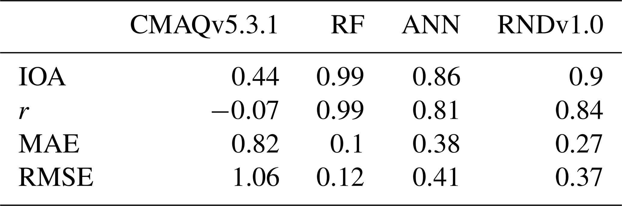
All models except CMAQ simulated the measured HONO mixing ratio fairly well (Fig. 5). CMAQ not only underestimated the measured HONO but also failed to represent its diurnal variation (Fig. 6). The statistical information about the performance of the four models is presented in Table 3. The mean measured HONO mixing ratio and those calculated using CMAQ, RF, ANN, and RNDv1.0 were 0.94, 0.09, 0.95, 0.88, and 0.89 ppbv, respectively. Of the four models, RF exhibited the best performance followed by RND. ANN advantageously calculates HONO more accurately than RND as it uses more input variables, but it has a lower data capture rate (41.5 %) compared to RND (97.7 %) or RF (85.3 %).

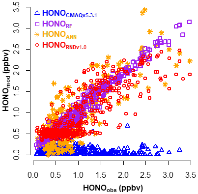
Figure 5 Comparison between the measured HONO (HONO_obs) and calculated HONO (HONO_mod) using CMAQv5.3.1 (blue triangle), RF (purple square), ANN (orange star), and RNDv1.0 (red circle) during the KORUS-AQ campaign (May–June 2016).

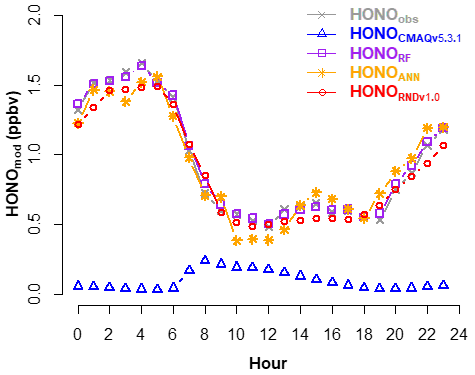
Figure 6 Average diurnal variation in the measured HONO (HONO_obs) and calculated HONO (HONO_mod) using CMAQv5.3.1 (blue triangle), RF (purple square), ANN (orange star), and RNDv1.0 (red circle) during the KORUS-AQ campaign (May–June 2016).

Table 3 Performance of the chemical transport model (CMAQv5.3.1) and machine learning (ML) models, including random forest (RF), artificial neural network (ANN), and RNDv1.0, on the measurement data from the 2016 KORUS-AQ campaign, which were used for training.

2.5 Model test

RNDv1.0 and the RF model were tested using data obtained in June 2018, April 2019, May–June 2021, and October–November in 2021, which were not used for RNDv1.0 training (Fig. 3). Note that the RF model outperformed the other three models in the training and validation process (Fig. 5). Although the performance of RNDv1.0 was slightly lower than that of the RF model, simulated and measured HONO mixing ratios were in good agreement. Interestingly, the performance of the RF model was much worse than RNDv1.0 in the testing process (Fig. 7). The IOA and correlation coefficient of the RF model were extremely low (0.29 and −0.02, respectively).

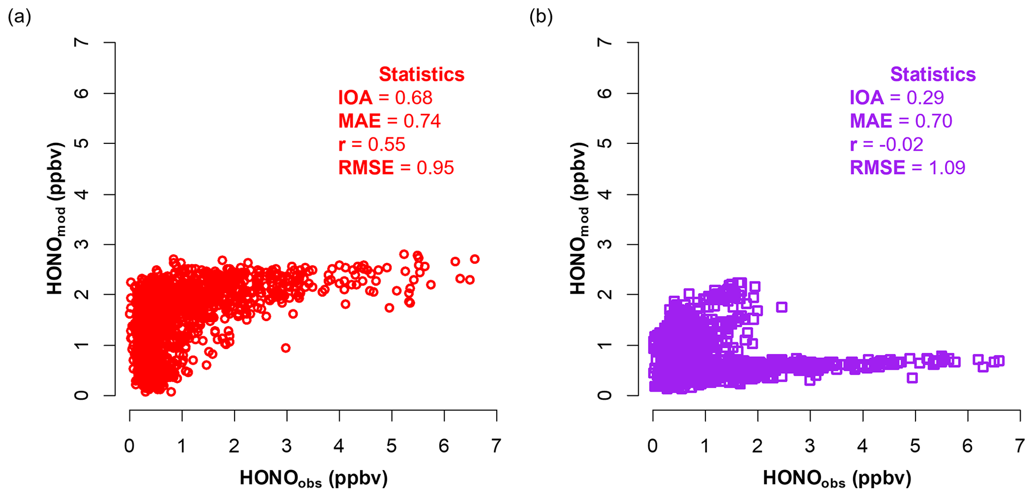
Figure 7 Relationship between measured HONO (HONO_obs) and modeled HONO (HONO_mod) using (a) RNDv1.0 and (b) a random forest model for the test dataset.

The performance of RNDv1.0 was slightly lower than that of the RF model, but it traced the HONO mixing ratio well. Among the test dataset, the early winter (October–November) data are particularly valuable for demonstrating the applicability of RNDv1.0 because they stem from different weather conditions than the training dataset. For example, HONO mixing ratios reached over 4 ppbv when the daily average PM_2.5 concentration increased to 120 µg m⁻³ during severe haze pollution events. Therefore, in the next step, the performance of RNDv1.0 was compared for the two cases by dividing the testing dataset into a group in which all input variables fall within the range of the training dataset and a group which does not meet this criterion. In RNDv1.0, there was no significant difference in performance between the two groups (Fig. S5 and Table S2). When the data in which at least one input variable does not fall within the range of the training dataset were excluded from the test dataset, no significant difference was observed in the performance of RNDv1.0 between the two that meet the same atmospheric conditions or do not meet the criteria (Fig. S5 and Table S2). These extreme atmospheric conditions can worsen the model performance. Except for these extremes, RNDv1.0 traced the variation in the HONO mixing ratio well. These results demonstrate the applicability of RNDv1.0, which is not strictly constrained by atmospheric conditions. The influence of the input variable is further analyzed in the next section.

2.6 Bootstrap test and feature importance

A simple bootstrapping test was conducted for both RNDv1.0 and the RF model to evaluate the relative importance of the input variable to the HONO estimates. In this analysis, each variable was set to zero, and MAE was calculated as an evaluation metric (Kleinert et al., 2021). Among the nine input variables of RNDv1.0, NO₂ was found to have the greatest influence on HONO concentration, followed by RH and T (Table 4). The highest MAE of 0.59 ppbv could be considered the maximum uncertainty of RNDv1.0 due to the input variable. The bootstrap test result agreed well with that of our previous study (Gil et al., 2021), where more variables such as aerosol surface area and mixing layer height were incorporated into the model, and it highlights the crucial role of precursor gases and heterogeneous conversion in HONO formation.

Table 4 Results of the bootstrap test of measurement data used to train the RF and RNDv1.0 models. The greater the MAE, the greater the influence of the variable.

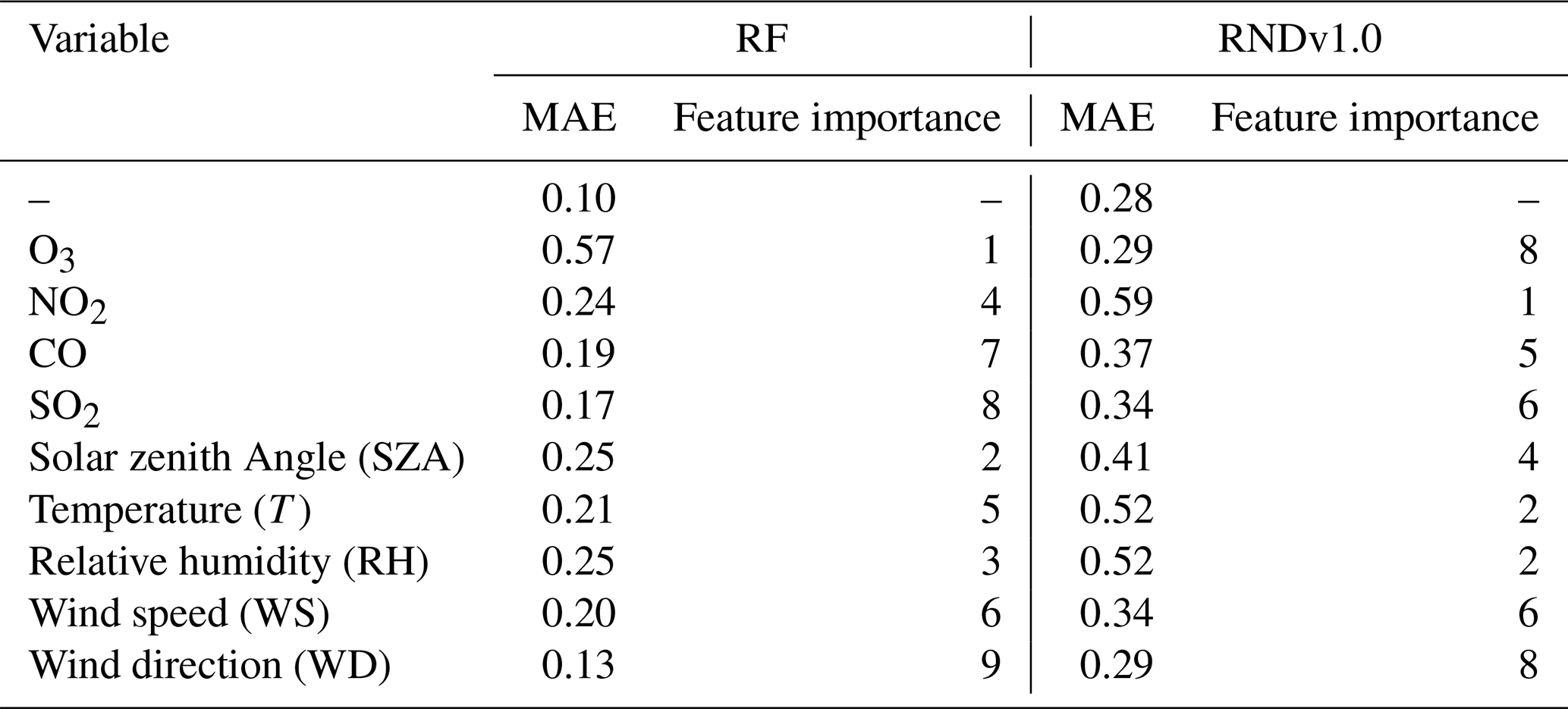
In contrast, in the RF model, O₃ was the most important variable. This is likely due to the distinct inverse relationship between O₃ and HONO in the diurnal patterns, as well as the O₃ variations over a wide range. In conjunction with the evaluation of the test dataset presented in the previous section, the results of the feature importance for the two models demonstrate the ability of RNDv1.0 to simulate the HONO mixing ratio more adequately in urban areas compared to the RF model. Thus, it is reasonable to state that RNDv1.0 constructed using routinely measured criteria pollutants and meteorological variables can sufficiently capture the HONO variability in the urban atmosphere.

3 Operation and application of RNDv1.0

The RNDv1.0 package is provided as an operational model, and the .h5 files can be opened in Python. To run RNDv1.0, the measurement data for nine input variables are required and need to be properly prepared, as described in Sect. 2.2. Once the input data are ready, open RNDv1.0 with the input data files using the code provided in the example (Fig. S3). Then, RNDv1.0 calculates and presents the HONO results as scaled values (x_sca), which then can be converted to the HONO mixing ratio (ppbv) via the two scale factors shown in Table 2 (Eq. 7):

$$\begin{array}{}\text{(7)}& \mathrm{HONO}\left(\mathrm{ppbv}\right)={\mathrm{HONO}}_{\mathrm{sca}}\times F_{\mathrm{1}}\left(\mathrm{HONO}\right)+F_{\mathrm{2}}\left(\mathrm{HONO}\right).\end{array}$$

The HONO calculated using Eq. (7) can be applied to an urban photochemical cycle simulation. As is already known, the photolysis of HONO is a major source of OH radicals in the early morning when the OH level is low, and this OH affects daytime O₃ formation through photochemical reactions with VOCs and NO_x, which are primarily emitted during the morning rush hour in urban areas. Furthermore, the OH produced from HONO promotes the photochemical oxidation of SO₂ and VOCs, leading to aerosol formation. However, the HONO formation mechanism is still poorly understood, which hinders the accurate simulation of O₃ and fine aerosols, as well as HONO, in conventional photochemical models.

The framework for 0-dimension atmospheric modeling (F0AM), which utilizes the MCM v3.3.1 chemical reaction mechanisms (Wolfe et al., 2016), can be used to simulate the diurnal variation in O₃ with the measurements of several reactive gases (NO, NO₂, CO, HCHO, VOCs, and HONO). Detailed information about F0AM can be found at https://sites.google.com/site/wolfegm/models (last access: 6 September 2023) and in previous studies (Gil et al., 2020; Wolfe et al., 2016). When the F0AM model is run without HONO, it is unable to reproduce the concentration and diurnal cycle of the observed O₃ (Fig. 8). In comparison, the model simulates the O₃ well within 2 ppbv when HONO is considered, which is the result of RNDv1.0. This is mainly due to the missing OH produced by HONO photolysis in the early morning. Its production rate is estimated to be 0.57 pptv s⁻¹, contributing approximately 2.28 pptv to the OH budget during 06:00–11:00 (local sun time) (Gil et al., 2021). Given that OH is mainly produced from the photolysis of O₃ under high sun, the early morning supply of OH from HONO photolysis will expedite the photochemical cycle involving NO_x and VOCs, promoting O₃ and secondary aerosol formation. The presence of HONO in the photochemical model allows for the accurate estimation of OH radicals; thus, the incorporation of RNDv1.0 into conventional models will improve their overall performance.

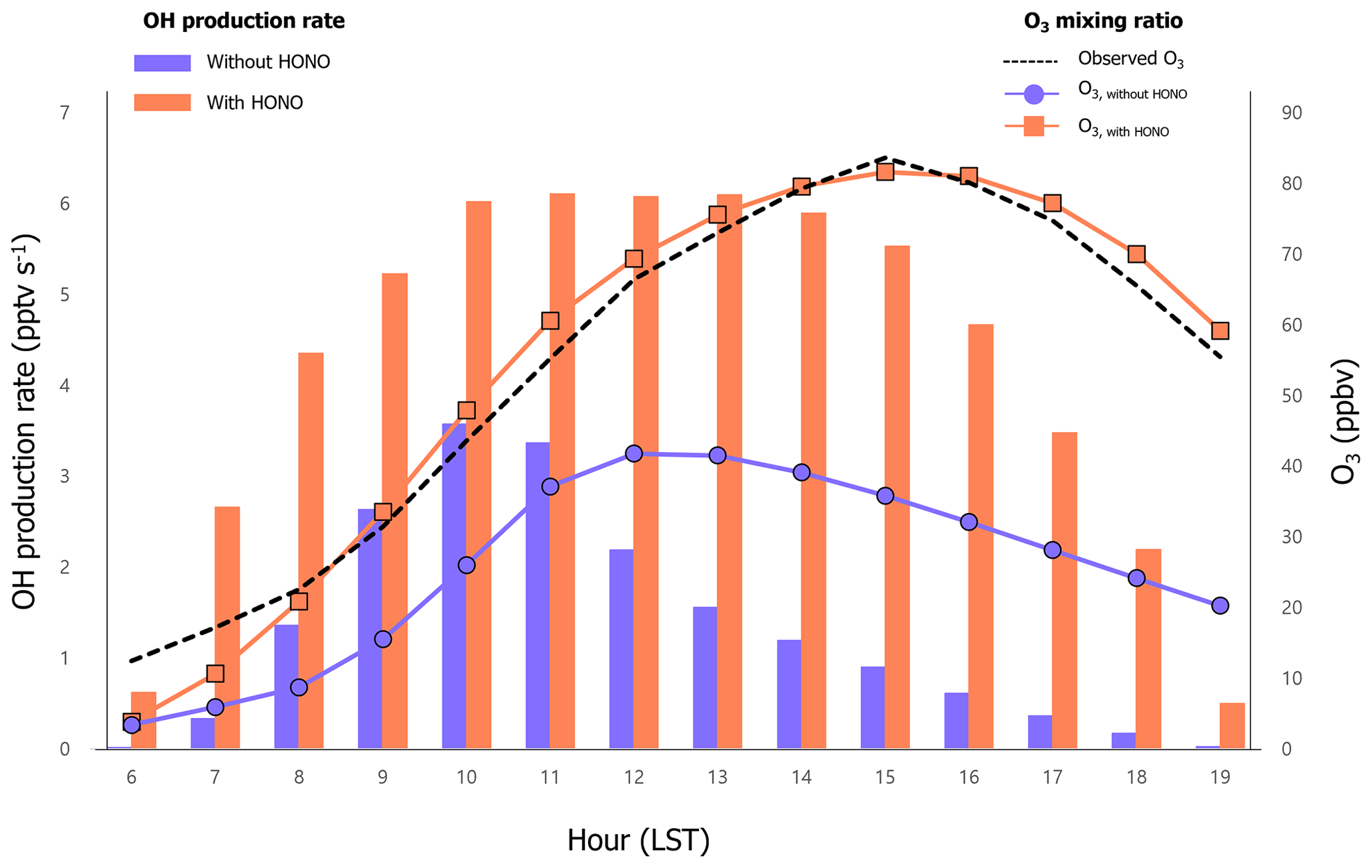
Figure 8 For June 2016, the diurnal variations in O₃ (line) and OH production rate (bar) calculated using the F0AM photochemical model with (orange) and without (blue) HONO estimated from the RNDv1.0 model. The measured and calculated O₃ values are compared.

4 Summary and implications

In this study, we developed the RND model to calculate the mixing ratio of NO_y in the urban atmosphere using a DNN along with measurement data. The target species of RNDv1.0 is HONO, and its mixing ratio is calculated using criteria pollutants, including O₃, NO₂, CO, and SO₂, as well as meteorological variables, including T, RH, WS, WD, and SZA. These variables are routinely measured through monitoring networks. RNDv1.0 was trained and validated using the HONO measurements data obtained in Seoul by adopting a KFCV method and tested with other HONO datasets. The test results demonstrate that RNDv1.0 adequately captures the characteristic variation in HONO.

RNDv1.0 was constructed using the measurements made in a high-NO_x environment, where the maximum NO₂ reached about 80 ppbv. During the measurement period, the HONO mixing ratio was increased up to about 7 ppb under the influence of air masses originating from China. When applying RNDv1.0 to regions or times heavily affected by transport, the model could possibly underestimate the HONO level without more detailed information, such as nanoparticles. Indeed, a previous study showed that HONO formation is closely related to the surface area of particles with diameters in the range of hundreds of nanometers (Gil et al., 2021). Nevertheless, RNDv1.0 is advantageously a relatively inexpensive test for measurement quality control and location selection, and it supports the data used for traditional chemistry models based on the current knowledge of the urban photochemical cycle. Therefore, RNDv1.0 can serve as a supplementary tool for conventional forecasting models. Attempts are currently being made to estimate ground HONO from satellite observations (Armante et al., 2021; Theys et al., 2020; Clarisse et al., 2011), and RNDv1.0 will be useful for validating the satellite-derived HONO.