J-GAIN v1.1: a flexible tool to incorporate aerosol formation rates obtained by molecular models into large-scale models

New-particle formation from condensable gases is a common atmospheric process that has significant but uncertain effects on aerosol particle number concentrations and aerosol–cloud–climate interactions. Assessing the formation rates of nanometer-sized particles from different vapors is an active field of research within atmospheric sciences, with new data being constantly produced by molecular modeling and experimental studies. Such data can be used in large-scale climate and air quality models through parameterizations or lookup tables. Molecular cluster dynamics modeling, ideally benchmarked against measurements when available for the given precursor vapors, provides a straightforward means to calculate high-resolution formation rate data over wide ranges of atmospheric conditions. Ideally, the incorporation of such data should be easy, efficient and flexible in the sense that same tools can be conveniently applied for different data sets in which the formation rate depends on different parameters. In this work, we present a tool to generate and interpolate lookup tables of formation rates for user-defined input parameters. The table generator primarily applies cluster dynamics modeling to calculate formation rates from an input quantum chemistry data set defined by the user, but the interpolator may also be used for tables generated by other models or data sources. The interpolation routine uses a multivariate interpolation algorithm, which is applicable to different numbers of independent parameters, and gives fast and accurate results with typical interpolation errors of up to a few percent. These routines facilitate the implementation and testing of different aerosol formation rate predictions in large-scale models, allowing the straightforward inclusion of new or updated data without the need to apply separate parameterizations or routines for different data sets that involve different chemical compounds or other parameters.

1 Introduction

Formation of secondary aerosol particles from condensable gases is a well-known and ubiquitous phenomenon in Earth’s atmosphere (Kerminen et al., 2018; Kontkanen et al., 2017). Aerosols have significant effects on climate and air quality, with the indirect climate effect through aerosol–cloud interactions forming the largest uncertainty in radiative forcing assessments (Szopa et al., 2021). New-particle formation, including the formation and condensational growth of nanoparticles from vapors, is an important factor affecting aerosol number concentrations and size distributions (Fountoukis et al., 2012; Makkonen et al., 2012; Gordon et al., 2017). The primary quantity characterizing the formation process is the initial particle formation rate J, often referred to as the nucleation rate, which gives the rate at which new particles of ca. 1–2 nm in diameter form per unit time and volume at given ambient conditions through clustering of vapor molecules. The chemical compounds that are able to drive and enhance the initial formation process include acids, bases, and organic species (Glasoe et al., 2015; Lehtipalo et al., 2018; Xiao et al., 2021). The roles and effects of different potentially important precursor vapors are not, however, resolved. While it is established that sulfuric acid (H₂SO₄) initiates particle formation in the presence of stabilizing species such as ammonia (NH₃) or monoamines (Jen et al., 2014; Almeida et al., 2013), there exist various species, such as diamines (Jen et al., 2016), organic acids (Zhang et al., 2004) and complex highly oxidized organic molecules (Kirkby et al., 2016), that may contribute to particle formation with or without sulfuric acid. Furthermore, quantitative particle formation rates are very challenging to assess: both theoretically and experimentally deduced formation rates involve high uncertainties (Almeida et al., 2013; Kürten et al., 2018) and may be sensitive to ambient conditions such as temperature and scavenging sink of the initial molecular clusters (Olenius et al., 2017; Elm et al., 2020).

The combination of quantum chemistry and molecular cluster dynamics simulations is the state-of-the-art method to calculate theoretical particle formation rates (Elm et al., 2020). Quantum chemistry is applied to compute the thermodynamics of the formation of the initial molecular clusters from vapor molecules. The thermochemistry data are converted to cluster evaporation rate constants and used as input in cluster population dynamics simulations, which determine the formation rate by modeling cluster formation and growth considering molecular collisions and evaporations and other dynamic processes such as cluster sinks (Olenius et al., 2013). Such simulations are fast and easy to perform, thus enabling the assessment of formation rates over wide ranges of atmospheric conditions for given chemical compounds. Benchmarking the theoretical methods against experimental data, which often cover a limited set of conditions, provides quality control and uncertainty estimates for the predicted formation rates (Almeida et al., 2013; Kürten et al., 2016).

New quantum chemical data, calculated for different chemical species (Elm et al., 2020; Elm, 2019a) or by applying different physical and computational approaches (Besel et al., 2020), are constantly becoming available. Such data can be used to test the effects of different particle formation mechanisms or improve quantitative formation rate predictions in atmospheric large-scale models. To this end, the formation rate data must be implemented as parameterizations or lookup tables (Dunne et al., 2016; Ehrhart et al., 2018; Kazil et al., 2010; Yu et al., 2020; Baranizadeh et al., 2016), as applying formation rate simulations within a large-scale model is not feasible. The formation rate is a function of several parameters, the most obvious of which are the concentrations of the vapors participating in the formation process and the temperature. In addition, formation rates obtained by cluster simulations include the effects of cluster sink caused by pre-existing larger aerosol particles and, depending on the chemical compounds and quantum chemical input data, possibly also atmospheric ions and relative humidity. In the presence of several cluster-forming vapors, particle formation can proceed through multicompound clustering or parallel clustering pathways involving non-interacting chemical mechanisms (Elm, 2019b).

Deriving parameterizations quickly becomes cumbersome as the number of independent parameters increases: finding parameterization formulas and coefficients that reproduce the formation rate data with a reasonable accuracy throughout the parameter space is virtually impossible for arbitrary chemical systems. Furthermore, evaluation of very complex formulas within a computationally heavy large-scale model may not be optimal. The benefit of lookup tables is that values determined from a table of sufficient resolution are guaranteed to be close to the original data, and no pre-processing of the formation rate data is needed. The use of such tables, on the other hand, requires multivariate interpolation algorithms that should ideally be applicable to tables of arbitrary dimensions, with no need for manual changes depending on the number of independent parameters. While interpolated values must be sufficiently accurate, the interpolation routine should be computationally efficient and preferably simple.

In this work, we introduce a tool to incorporate molecular modeling data in atmospheric models by flexible routines to generate and interpolate formation rate lookup tables. With this approach, we aim to cover the following aspects:

• flexible implementation of state-of-the-art molecular modeling results in large-scale models;

• inclusion of arbitrary chemical compounds;

• efficient multivariate interpolation; and

• user-friendly routines with no need for modifications depending on, for instance, included chemical compounds.

We construct a lookup table generator that embeds a publicly available cluster dynamics model to calculate formation rates from user-defined quantum chemistry input data and provide a table interpolation routine that can be readily implemented in a large-scale model. The table generator enables easy application of the standard formation rate modeling approach, but the interpolator can also be used for tables saved from other models in the same, simple format. We present assessments of optimal table resolution and interpolation accuracy and demonstrate the use and performance of the tool by application on sulfuric acid–ammonia cluster chemistry data. We generate tables suitable for global applications for these data and assess the performance of the interpolation routine in typical computationally heavy model setups.

2 Methods

The proposed lookup table approach comprises two components: a generator routine to create tables and an interpolation routine to be implemented in an atmospheric model. We refer to the routines as J-GAIN (Formation rate (J) lookup table Generator And INterpolator). The details of the generation and interpolation routines are presented in Sect. 2.1 and 2.2, respectively, and their application is further discussed in Sect. 2.3 and 2.4. The table generator primarily uses input data from quantum chemical calculations and calls a molecular cluster dynamics model to determine the formation rates, as this is the standard method in theoretical atmospheric particle formation studies. The interpolation routine can, however, also be applied to formation rate data obtained by other means by saving the tabulated data in the given table format. Figure 1 shows a schematic presentation of the J-GAIN routines, summarizing the input, output and usage. J-GAIN is written in Fortran, with the exception that the cluster dynamics model used by the table generator applies also Perl, and licensed under GPL 3.0. The code repository includes detailed instructions for using the programs (Yazgi and Olenius, 2023a, b).

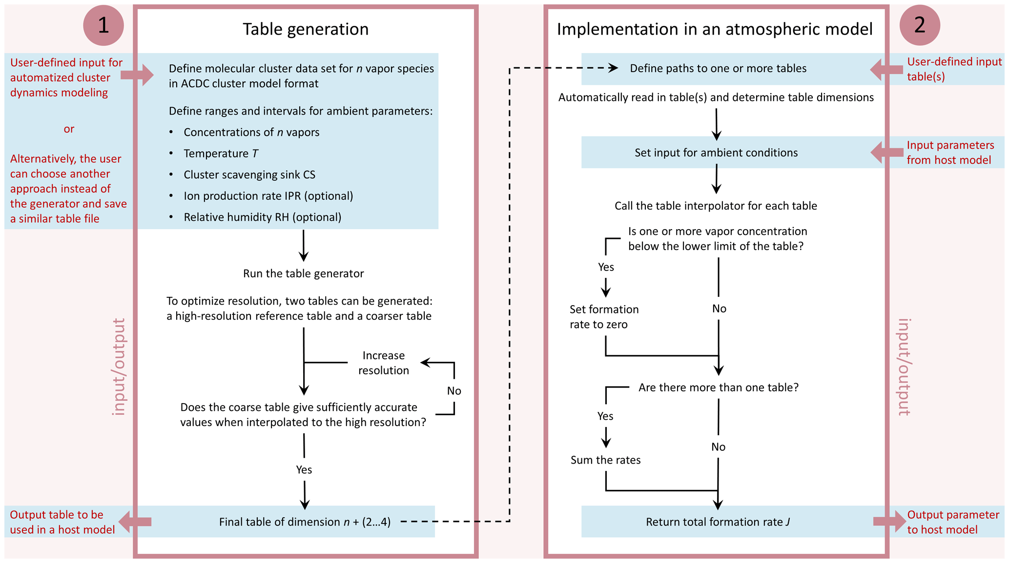
Figure 1 Flow chart illustrating the generation and application of particle formation rate tables by J-GAIN. The boxes summarize the steps for using the two parts: (1) table generation with automatized calculation of formation rates by cluster dynamics modeling and (2) implementation of tables and the table interpolator in a host model. User-defined input and output are specified outside the boxes.

2.1 Table generation

By default, the table generator takes molecular cluster thermochemistry data for the given chemical compounds as input and calculates the formation rates by molecular cluster dynamics simulations through coupling to the open-source cluster model ACDC (Atmospheric Cluster Dynamics Code; Olenius, 2021). In practice, application of the generator on a new cluster data set consists of two steps: creating the formation rate equations by ACDC and running the generator to obtain the table (see Yazgi and Olenius, 2023a). As the embedded ACDC application provides automatized and flexible treatment of arbitrary cluster data sets, we recommend the default table generator when applying the commonly used combination of quantum chemical input and cluster dynamics modeling to obtain formation rates. It can be noted that ACDC also includes a wide selection of options that increase the flexibility: for example, while cluster evaporation rate constants are by default obtained from the thermochemistry data, they can also be given as direct input if the user wishes to assess them in some other way. The advanced user may also modify other cluster simulation settings (see the ACDC manual; Olenius, 2021). However, the table interpolator is not limited to tables generated by the default table generator, and thus it is possible to use alternative approaches to determine formation rates. For this, the rates must be saved in the same file format as that produced by the default generator, as detailed in Appendix A.

In addition to the molecular cluster data, the table generator requires user-defined input for the ranges of the parameters that define the ambient conditions. These parameters include the concentrations of the vapor compounds, temperature (T), coagulational scavenging sink (CS; given as vapor condensation sink which is scaled for different cluster sizes within the cluster dynamics model as derived by Lehtinen et al., 2007), and optionally also ion production rate (IPR; given as generic ion pairs per unit volume and time) and relative humidity (RH). This gives n+(2…4) independent parameters, where n is the number of chemical compounds. While vapor concentrations, temperature and cluster sink always affect the particle formation rate and are thus included by default, the inclusion of IPR and RH depends on the chemical system and also on data availability. For strongly clustering chemistries, ion effects may be negligible (Myllys et al., 2019), and RH effects may also be minor (Henschel et al., 2016). As the addition of charged species and hydrates in a quantum chemistry data set requires a significant computational effort, these effects are not always included in available thermochemistry data sets.

The user sets the range for the values of each parameter by giving the lower and upper limits, and the number of values to be placed within the limits at even intervals. Parameters can be defined as “logarithmic”, in which case the data points are placed evenly on a logarithmic scale. This is relevant for, for example, vapor concentrations. The formation rate table is then generated by running the generator which calls ACDC to obtain the formation rate J for each combination of parameter values.

The tables are outputted as binary files, and a descriptor file is generated together with the table. The latter contains the essential information on the table, including the names and units of the independent parameters, the lower and upper limits of the parameter values, and the numbers of values along each dimension. In order to ensure sufficient accuracy, several tables can be generated at different resolutions. Then, possible errors in interpolated values can be assessed by interpolating a coarser-resolution table on the grid of a higher-resolution reference table (Sect. 3.1).

2.2 Table interpolation

The interpolation routine uses the descriptor file to obtain the number and identities of the independent parameters for the corresponding lookup table. After loading the table, the routine determines the formation rate by linear multivariate interpolation. In general, for an N-dimensional function $f=f(x_{\mathrm{1}},x_{\mathrm{2}},\mathrm{\dots },x_N)$ with nearest known data points at locations x_j,0 and x_j,1 for each variable x_j, where $x_{j,\mathrm{0}}<x_{j,\mathrm{1}}$ and $j=\mathrm{1},\mathrm{\dots },N$, the interpolated value $\stackrel{\mathrm{̃}}{f}$ can be written as

$$\begin{array}{}\text{(1)}& \begin{array}{rl}& \stackrel{\mathrm{̃}}{f}\left(x_{\mathrm{1}},x_{\mathrm{2}},\mathrm{\dots },x_N\right)=\sum _{(i_{\mathrm{1}},i_{\mathrm{2}},\mathrm{\dots },i_N)\in \mathit{\{}\mathrm{0},\mathrm{1}{\mathit{\}}}^N}\\ & \cdot f\left(x_{\mathrm{1},i_{\mathrm{1}}},x_{\mathrm{2},i_{\mathrm{2}}},\mathrm{\dots },x_{N,i_N}\right)\prod _{j=\mathrm{1}}^N\left\{\begin{array}{ll}{x}_j^{\prime },& i_j=\mathrm{1}\\ \mathrm{1}-x_j^{\prime },& i_j=\mathrm{0}\end{array}\right.,\end{array}\end{array}$$

where the summation goes over the values of f at all combinations of points x_j,0 and x_j,1 for $j=\mathrm{1},\mathrm{\dots },N$, and

$$\begin{array}{}\text{(2)}& x_j^{\prime }={\displaystyle \frac{x_j-x_{j,\mathrm{0}}}{x_{j,\mathrm{1}}-x_{j,\mathrm{0}}}}.\end{array}$$

Here, we perform linear interpolation by default for f=log J and either x_j or log x_j depending on if parameter j is defined as linear or logarithmic, respectively. This gives more accurate results than assuming purely linear relationships, as J generally varies smoothly on a logarithmic scale. Moreover, a linear dependence between the logarithms of J and the concentration C of a contributing vapor within a short interval along the C axis is also expected based on simplified cluster formation theories (see, e.g., Li and Signorell, 2021). The choices of applying either the actual values or the logarithms of the dependent and independent parameters can also be changed by the user.

Treatment of input values that are outside the ranges covered by the table is parameter-dependent and defined by the user. For each parameter, the following options are included in the example routines.

1. Value below/above the table limits → the value is set to the lower/upper limit of the table (this is the default behavior).

2. Value below the lower limit → J=0 is returned; input value above the upper limit → the value is set to the upper limit.

The latter option is for vapor concentrations, provided that the lower limits of the table are chosen so that effectively no particle formation is expected at concentrations below the limits. The first option is by default used for other parameters.

2.3 Incorporation of tables in a host model

In the code repository, we provide an example of simple interfaces to load and interpolate lookup tables within a host model. The input parameters of the interpolation subroutine include all independent parameters that the particle formation rate may depend on, and the total formation rate is returned as output. Importantly, the interpolator is not limited to using a single table: separate particle formation pathways, corresponding to different chemical compounds, can be incorporated as separate tables. If more than one table is used, the interpolator is applied separately to each table, and the total formation rate can be obtained as the sum of the individual formation rates.

The repository includes a simple example of summing the rates interpolated from two separate tables. However, the user may construct different ways to treat several tables according to their needs and data availability. To give an example, a possible practical application could be as follows: separate tables are used for parallel formation mechanisms, for example, inorganic H₂SO₄–base and organics-driven pathways. There may also be alternative tables that are selected based on the presence of a given chemical species, that is, if the concentration of the species is high enough for the species to contribute. For instance, there may be data for particle formation from H₂SO₄ and NH₃ with or without an amine species. In the presence of the amine, a table of H₂SO₄–NH₃–amine formation rates is selected for the H₂SO₄–base pathway, while otherwise a H₂SO₄–NH₃ table is applied. This example of a potential table combination is schematically presented in Fig. 2.

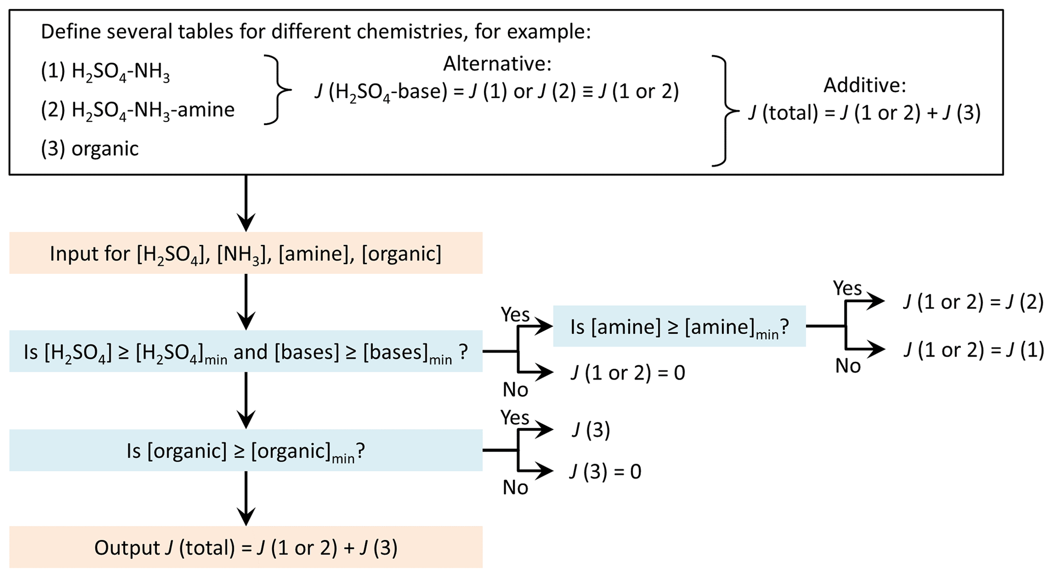
Figure 2 Schematic presentation of treatment of several tables: an example of a possible table combination that the user may construct according to their needs.

2.4 Example case: sulfuric acid–ammonia particle formation

We demonstrate the application and performance of the J-GAIN table generator and interpolator using previously published quantum chemical data for sulfuric acid and ammonia (Olenius et al., 2013), which are common atmospheric particle formation precursor vapors. Here, the input molecular cluster data for the H₂SO₄–NH₃ chemistry includes charged clusters but no hydration, and therefore the independent parameters that determine the formation rate are vapor concentrations [H₂SO₄] and [NH₃], T, CS and IPR.

We apply the H₂SO₄–NH₃ cluster data to generate tables of different resolution and coverage. First, we demonstrate the effect of table resolution by generating tables that cover subsets of independent parameter ranges where J is sensitive to the parameter values and compare the interpolated values of J to accurate values given by a high-resolution reference table. Second, we generate extended tables suitable for global applications, where the ranges of all independent parameters cover various environments from the boundary layer to the upper troposphere. The extended tables are applied to evaluate the accuracy of J interpolated over the full set of parameters [H₂SO₄], [NH₃], T, CS and IPR that follow representative diurnal cycles, corresponding to practical model implementations. To assess the performance of the interpolation routine for given table sizes, we determine the interpolation speed for test tables of different numbers of data points and dimensions.

3 Results and discussion

3.1 Effect of table resolution on accuracy

Figure 3 presents J interpolated along the [H₂SO₄] axis and the error in the interpolated values at representative atmospheric conditions for tables with ${\mathrm{2}}^k+\mathrm{1},k=\mathrm{4}\mathrm{\dots }\mathrm{9}$ data points on the axis. That is, for each subsequent table the number of points is doubled, resulting in numbers ranging from 17 to 513. For the lowest resolution of ${\mathrm{2}}^{\mathrm{4}}+\mathrm{1}=\mathrm{17}$ points, the relative error is less than ±10 %, and for $\ge {\mathrm{2}}^{\mathrm{6}}+\mathrm{1}=\mathrm{65}$ points the error is well below ±1 %. Figure 4 shows the error as a function of both [H₂SO₄] and [NH₃] at two different temperatures for the two lowest resolutions used here. For ${\mathrm{2}}^{\mathrm{4}}+\mathrm{1}=\mathrm{17}$ points along both axes, the error is up to 10 % but mostly below it, and doubling the resolution to ${\mathrm{2}}^{\mathrm{5}}+\mathrm{1}=\mathrm{33}$ points drops the error below a couple of percent.

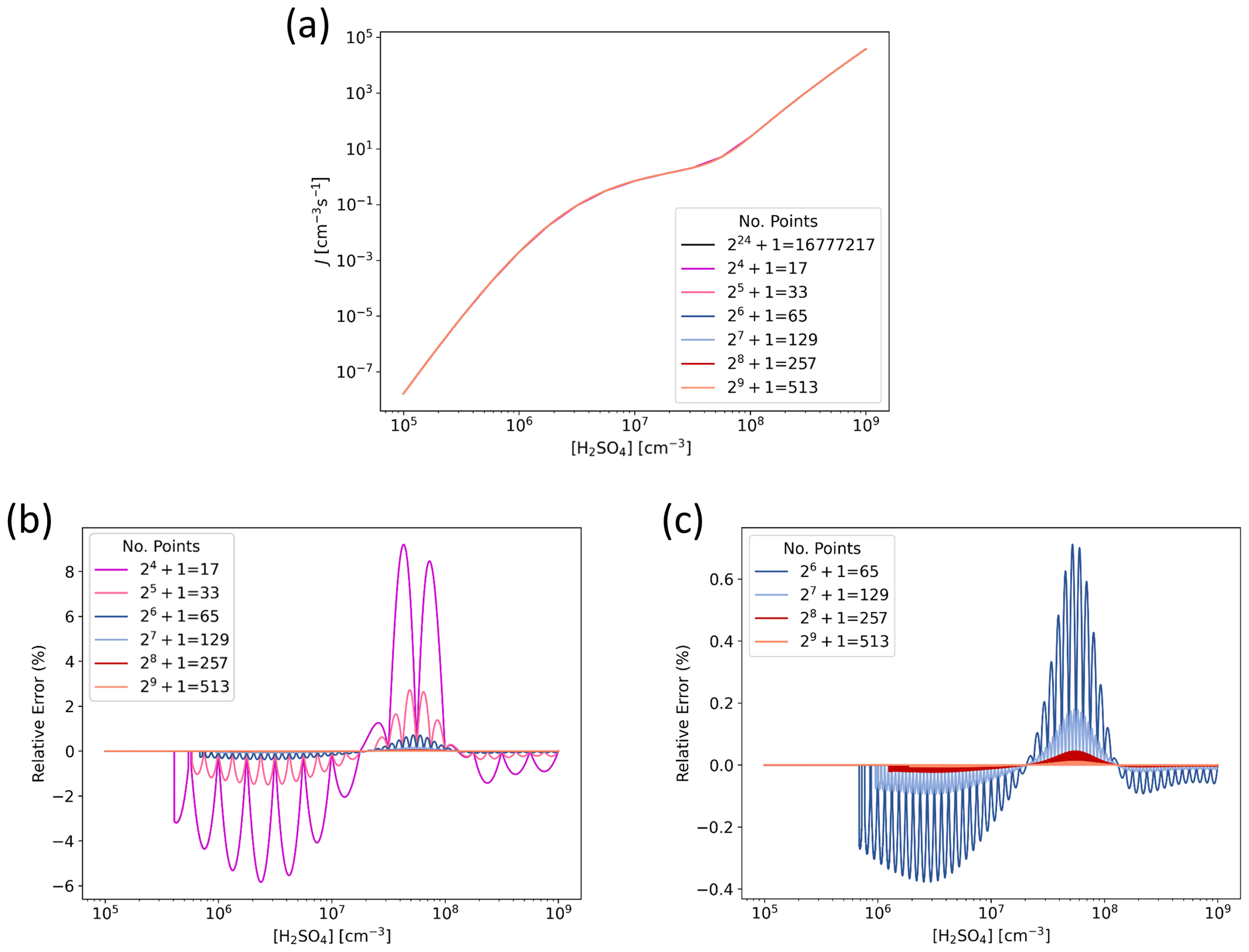
Figure 3 Particle formation rate J as a function of H₂SO₄ concentration for H₂SO₄–NH₃ model chemistry ([NH₃] =10¹⁰ cm⁻³, T=298.15 K, CS $={\mathrm{10}}^{-\mathrm{3}}$ s⁻¹, IPR =3 cm⁻³ s⁻¹), determined from lookup tables of different resolution. (a) Absolute J. Note that the different lines mostly fall on top of each other. (b) Relative error in interpolated J compared to accurate values given by the highest-resolution reference table with ${\mathrm{2}}^{\mathrm{24}}+\mathrm{1}\sim \mathrm{2}\times {\mathrm{10}}^{\mathrm{7}}$ points along the [H₂SO₄] axis. (c) Relative error in interpolated J for resolutions of $\ge {\mathrm{2}}^{\mathrm{6}}+\mathrm{1}=\mathrm{65}$ points.

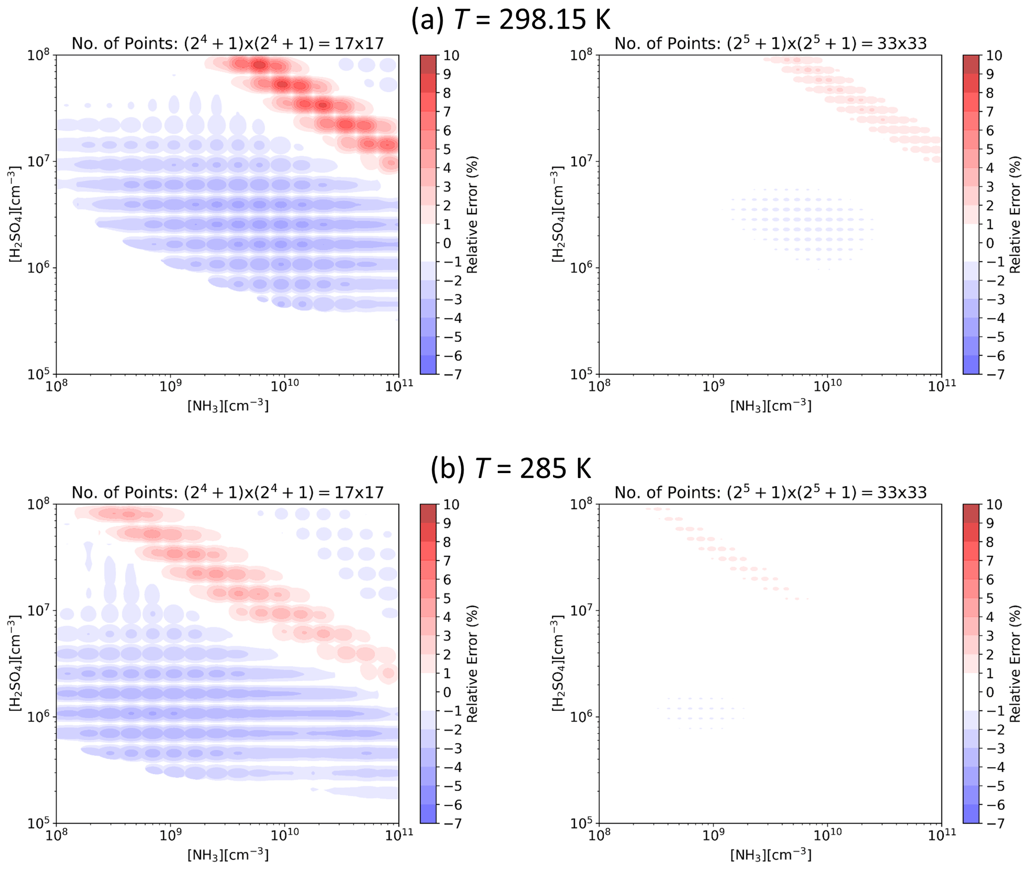
Figure 4 Relative error in interpolated particle formation rate J as a function of H₂SO₄ and NH₃ concentrations for lookup tables with ${\mathrm{2}}^{\mathrm{4}}+\mathrm{1}=\mathrm{17}$ and ${\mathrm{2}}^{\mathrm{5}}+\mathrm{1}=\mathrm{33}$ data points along the [H₂SO₄] and [NH₃] axes at CS $={\mathrm{10}}^{-\mathrm{3}}$ s⁻¹ and IPR =3 cm⁻³ s⁻¹ and (a) T=298.15 K and (b) T=285 K.

In order to demonstrate the application of the interpolator for interpolation over all independent parameters at realistic ambient conditions, corresponding to implementation of the routine in an atmospheric model, J is determined for a representative diurnal cycle as shown in Fig. 5. The independent parameters are set to follow 24 h time profiles as described in Appendix B. Here, we apply extended tables that cover wide ranges of parameter values, suitable for larger-scale chemical transport or general circulation models: [H₂SO₄] =10⁵–10⁸ cm⁻³, [NH₃] $={\mathrm{10}}^{\mathrm{6}}-\mathrm{3}\times {\mathrm{10}}^{\mathrm{11}}$ cm⁻³, T=180–320 K, CS $={\mathrm{10}}^{-\mathrm{5}}$–10⁻¹ s⁻¹, and IPR =0.1–60 cm⁻³ s⁻¹. The errors in Fig. 5 are generally of the same order as in Figs. 3 and 4 although somewhat higher due to interpolation over all parameters. Doubling the table resolution from ${\mathrm{2}}^{\mathrm{4}}+\mathrm{1}=\mathrm{17}$ to ${\mathrm{2}}^{\mathrm{5}}+\mathrm{1}=\mathrm{33}$ points (1) only for vapor concentrations and (2) for all parameters decreases the maximum errors down to ca. ±15 % and well below ±10 %, respectively. The errors are similar when using different absolute values of the independent parameters, tested by modifying the diurnal profiles by scaling the parameter values up or down (by, e.g., an order of magnitude for vapor concentrations or CS).

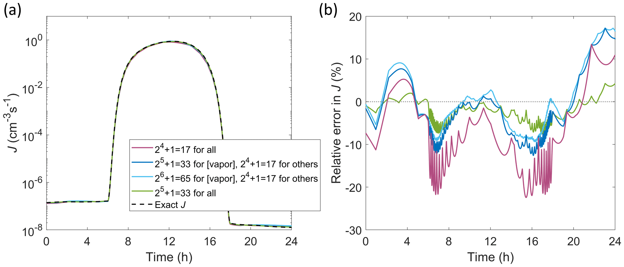
Figure 5 Particle formation rate J for a diurnal cycle in which all independent parameters [H₂SO₄], [NH₃], T, CS and IPR vary with time (Appendix B). (a) Absolute J. (b) Relative error in interpolated J compared to accurate values. Interpolated values are determined from the extended tables with increasing resolution either along only vapor concentration axes or along all axes as indicated in the legend.

In general, such errors are very small compared to typical uncertainty estimates for formation rate data: uncertainties in both theoretical and experimental J generally span up to an order of magnitude and beyond (see, e.g., Kürten et al., 2016). Based on the present evaluations, the interpolation approach is not expected to add notable uncertainties in the formation rate representation even at the lowest resolutions applied. Moreover, the accuracy is significantly increased by doubling the resolution. However, it can be noted that high-resolution tables quickly become very large, and the interpolation speed may be affected by the number of data points along the dimensions. Therefore, the choice of resolution depends on (1) the desired accuracy, (2) the size of the tables the user is willing to generate and store, and (3) the computational aspects of the model application considering the number of calls to the interpolator (Sect. 3.2).

3.2 Effect of table size and number of independent parameters on performance

In order to assess the interpolation speed with respect to the numbers of data points and independent parameters, we apply arbitrary test tables of different sizes and dimensions. Figure 6 shows the mean run time for 1 million calls to the interpolator with randomly assigned input parameter values. Here, the x axis is the base-2 logarithm of the table size (total number of values in the table). Therefore, for a table with equal numbers of points 2^k+1 along all dimensions, the x axis corresponds to approximately N×k, where N is the number of dimensions.

The performance is primarily affected by the number of dimensions: the addition of a new dimension may increase the run time by up to a factor of ∼2. In addition, the run time exhibits a major increase when the table size becomes very large, here beyond ca. 2²⁸ (of the order of ≳10⁸) data points. This is due to memory limits and management, and thus the exact threshold size depends on the computing system. For example, for the H₂SO₄–NH₃ table with N=5 and the current simple test setup with 64 GiB memory on the node, the threshold of ∼2²⁸ points corresponds to k>5. In the case that managing very large tables becomes slow on a given system, the performance can be optimized by splitting the table into subtables that cover different parts of the ambient conditions parameter space.

The approximative run times of Fig. 6 can be compared to typical overall times for, e.g., global-scale applications. We have implemented the H₂SO₄–NH₃ table for first tests in the EC-Earth climate model (Döscher et al., 2022). In this EC-Earth setup, the total number of grid points where the interpolation routine is called is 367 200 (120×90 horizontal grid points and 34 vertical layers), the time step for determining the formation rate is 1 h, and the chemistry model uses 90 processes. This corresponds to approximately ≲1 min run time for the formation rate routine for a simulation of 1 year, assuming a mean time of ≲2 s for 10⁶ lookups (Fig. 6, resolutions of ${\mathrm{2}}^{\mathrm{4}}+\mathrm{1}=\mathrm{17}$ and ${\mathrm{2}}^{\mathrm{5}}+\mathrm{1}=\mathrm{33}$ for all axes). Such a contribution can be considered acceptable compared to the overall model run time of ≳10 h per year or to the contribution of the atmospheric chemistry component, which accounts for up to even ∼90 % of the total run time (van Noije et al., 2014).

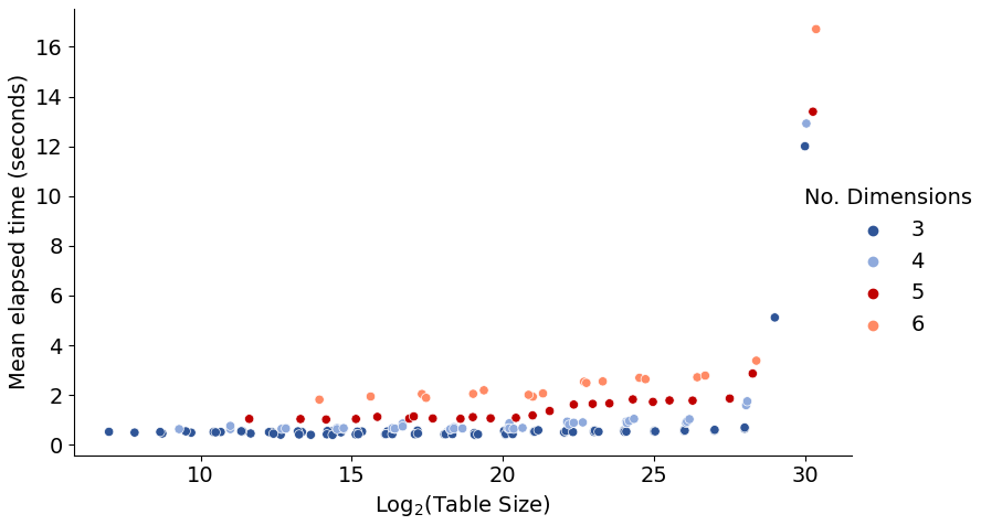
Figure 6 Time required to perform 1 million lookups for tables of different sizes. The figure shows different combinations $({\mathrm{2}}^k+\mathrm{1},{\mathrm{2}}^l+\mathrm{1},{\mathrm{2}}^m+\mathrm{1},..)$ of data points along axes, keeping k=l and the total number of points $<({\mathrm{2}}^{\mathrm{7}}+\mathrm{1}{)}^{\mathrm{2}}({\mathrm{2}}^{\mathrm{4}}+\mathrm{1}{)}^{\mathrm{4}}\sim {\mathrm{2}}^{\mathrm{30.37}}$. For more details, see discussion in Sect. 3.2.

For applications with, e.g., higher spatial resolution or shorter time step, the performance of the formation rate routine can be optimized by reasonable choices of table dimensions and size. For example, for very strongly clustering chemical systems, the presence of atmospheric ions only has minor effects. The IPR parameter could thus be discarded in the interest of speed. In addition to the resolution of the independent parameter values (i.e., the absolute intervals), their ranges (minimum and maximum values) can also be chosen considering the modeled environment, so that redundant values are avoided. If the numbers and ranges of parameters cannot be optimized further, very large tables can be divided into separate subtables that cover different sets of ambient conditions and selected within the host model application based on the input conditions.

It can also be noted that considering the high accuracy of the interpolated values, interpolation from pre-generated tables is superior compared to the time required to calculate the formation rates by the molecular cluster model. For example, generating the table of $({\mathrm{2}}^{\mathrm{4}}+\mathrm{1}{)}^{\mathrm{5}}=\mathrm{1419857}$ data points takes 27 h on a single process, corresponding to a mean time of ca. 0.068 s per value. Such times would be infeasible for operational models.

3.3 Potential limitations in applying formation rates in a host model

It must be noted that incorporating aerosol formation rates in an atmospheric model involves given limitations. These limitations are independent of the data source or implementation method and apply equally to lookup tables, parameterizations or other approaches. An obvious restriction is the availability of tracers in the host model. While various chemical compounds may contribute to atmospheric particle formation, including large numbers of new species in a chemical transport model may be cumbersome. In addition, sources of individual chemical species, such as different types of amines or organic acids, may not be well quantified.

Here, we apply particle formation rates from H₂SO₄ and NH₃, which are common species included in atmospheric models, and comprise a central particle formation pathway according to current understanding (Dunne et al., 2016; Gordon et al., 2017). Tables generated in this work can thus be easily implemented in standard models that include aerosol formation processes. On the other hand, H₂SO₄–amine particle formation, for example, requires the inclusion of amine species which are not common tracers despite their potential importance to aerosol formation (Bergman et al., 2015). Different types of amines may exhibit different particle formation efficiencies, but some amine species are similar in terms of their effects on the formation rate (Jen et al., 2014; Olenius et al., 2017). In order to test the importance of such particle formation agents in a large-scale model, some simplifications are often needed.

A simplified option to include rough source–sink dynamics for species that can be assumed to have common sources and similar properties with respect to gas-phase chemistry and gas-to-particle partitioning is to implement a lumped or representative trace compound. For example, monoamines with similar properties – namely di- and trimethylamines – have been approximated as a single representative alkylamine species, the emissions of which are scaled from ammonia emissions by assumed amine-to-ammonia ratio due to their common sources (Bergman et al., 2015). To take into account possible differences in the particle formation rates due to different amines, an option is to estimate the contributions of individual species based on available measurements (Schade and Crutzen, 1995). Oxidized organic species can be treated in a similar manner through a representative highly oxidized, ultra/extremely low-volatile compound (generally referred to as HOM or ULVOC/ELVOC; Kirkby et al., 2016; Schervish and Donahue, 2021), which is already included in some transport models (Gordon et al., 2017; Julin et al., 2018; Patoulias and Pandis, 2022).

In addition, it can be noted that the standard approach to implement formation rates involves certain approximations related to molecular cluster kinetics. Namely, formation rates are assumed to be determined solely by ambient conditions, applying the steady-state approximation for the cluster population and omitting time-dependent vapor–cluster–aerosol kinetics (Yu, 2003; Olenius and Riipinen, 2017; Olenius and Roldin, 2022). While such simplifications are needed for large-scale applications, they may affect the secondary particle concentrations. To minimize such effects, it can be recommended to extend the modeled aerosol size distribution to as small sizes as achievable instead of extrapolating the formation rate to a substantially larger size (Lee et al., 2013),or to apply a more detailed size distribution representation on the smallest particle sizes (Blichner et al., 2021). Nevertheless, the inherent steady-state assumption in the initial formation rate at ca. 1 nm is likely to cause overprediction in the case of strongly clustering, low-concentration trace species, and thus the rate should be considered as an upper-limit estimate for such chemistries (Olenius and Roldin, 2022).

4 Conclusions

Adequate representation of aerosol particle formation from vapors in atmospheric models is needed for assessing the climate and health effects of aerosols. The increasing amount of available computational molecular cluster chemistry data enables calculation of new-particle formation rates for different chemical compounds and computational chemistry methods. As formation rates are typically complicated functions of ambient conditions, a practical approach to apply them in an atmospheric model framework is through lookup tables. Here, we provide a tool to generate and interpolate formation rate tables, applicable to arbitrary sets of chemical species, for conveniently incorporating theoretical particle formation rate data in large-scale models.

Tests conducted using data for H₂SO₄–NH₃ particle formation show that the interpolation approach is efficient and accurate, with maximum interpolation errors typically ranging from negligible to ca. ± 10 %–20 % depending on table resolution. Interpolation errors can also be minimized by choosing to interpolate given parameters on a logarithmic instead of a linear scale. As interpolation speed is affected by the number of independent parameters and also by the table size for very large tables, the choice of parameters and the resolution should be optimized considering the computational burden of the application where the table is implemented. For heavy applications, redundant independent parameters that have only minor effects on the formation rate can be discarded, and the number of data points along each dimension can be set according to the desired accuracy. The flexibility of the provided tool makes the routines easy to apply to different data sets and choices of table dimensions and size. This design facilitates data transfer between the molecular modeling and the large-scale modeling communities.

Appendix A: Data sources and table format

For J-GAIN, formation rate tables can be created (1) by the provided table generator when applying the molecular cluster dynamics modeling approach or (2) by saving tabulated formation rates from another data source in a similar table. The details of the formats are listed below, and detailed instructions for the table generator are available in the J-GAIN repository (Yazgi and Olenius, 2023a).

For the J-GAIN table generator, the molecular cluster input data are given in the format of the ACDC model. Briefly, the set of input files include

1. molecular compositions of the clusters

2. cluster formation free energies as enthalpies and entropies, and

3. cluster dipole moments and polarizabilities if charged species are also included.

These files are summarized in the J-GAIN repository where also example files for the present test case can be found (Yazgi and Olenius, 2023a, ACDC subdirectory) and described in detail in the ACDC technical manual (Chap. 3) available in the ACDC repository (Olenius, 2021). Before applying the table generator, the user creates the ACDC formation rate equations for the given input by running the program provided in the J-GAIN repository. This gives the standard model setup, although it can be noted that the advanced user may also adjust the cluster modeling settings within the program if wanting to, for example, modify rate constants (ACDC manual, Chap. 2.5). Lastly, for running the table generator, the user sets the ranges of the ambient conditions in the namelist file (template provided in the generator subdirectory).

For other data sources, the data need to be processed into the table format applied by the J-GAIN interpolator, including two files:

1. a binary file that contains the formation rate array and

2. a descriptor file that lists the independent parameters and their ranges.

The rates are saved in the binary file as a flattened 1-dimensional array that can be constructed by iterating over the independent parameter values in a nested loop. The order of the parameters in the nested loop must be the same as that in the descriptor file. That is, if the descriptor file lists parameters x₁, x₂, …, x_N, in this order, the outermost loop must correspond to x₁ and the innermost to x_N (Algorithm A1).

Algorithm A1 Order of loops over the values of the independent parameters for saving a lookup table in the J-GAIN format (see Appendix A for details).

i=0

for i₁=1 to i_max,1 do

…

for i_N=1 to i_max,N do

$i=i+\mathrm{1}$

Save $f\left(i\right)=f(x_{\mathrm{1},i_{\mathrm{1}}},x_{\mathrm{2},i_{\mathrm{2}}},\mathrm{\dots },x_{N,i_N})$

end for

…

end for

In Algorithm A1, i_j is the index corresponding to values given for parameter x_j, and i_max,j is the total number of values for x_j. Example codes for such loops are included in the J-GAIN repository. The descriptor file can be created by following the instructions and example files in the repository (table generator subdirectory).

Appendix B: Parameter descriptions in the diurnal test case

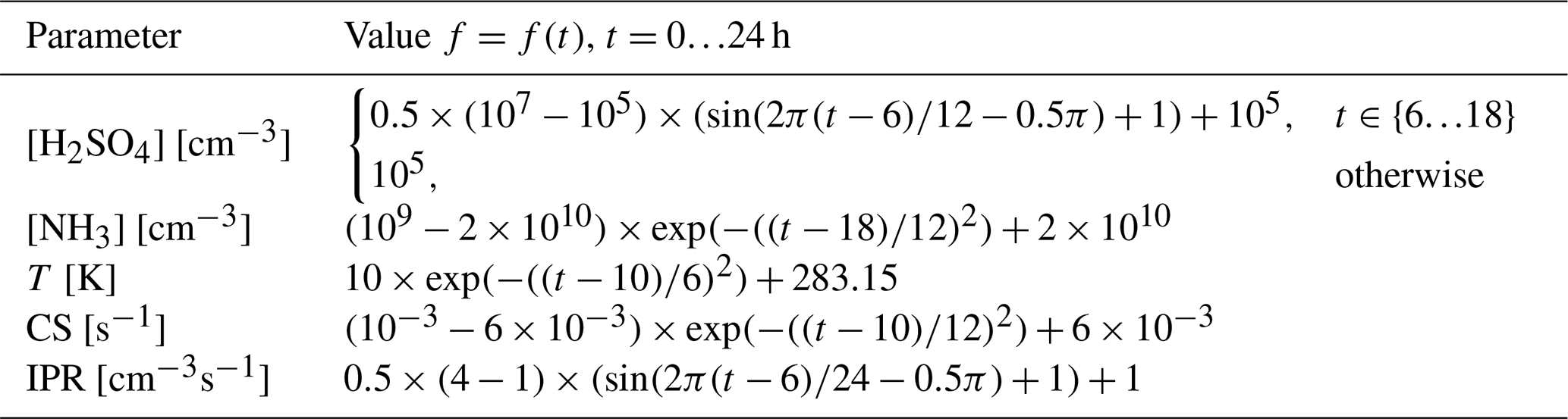
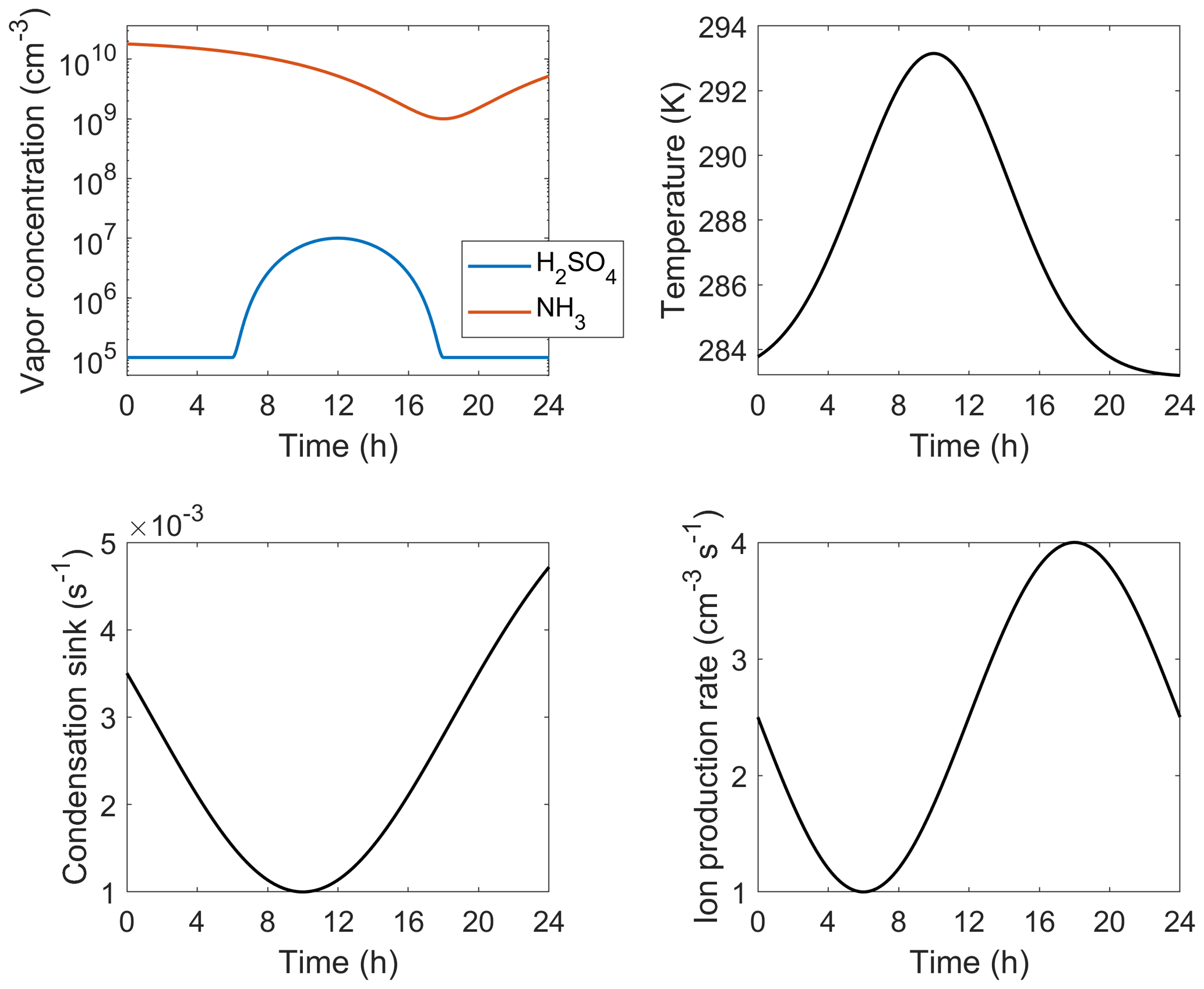
Table B1 lists the functional forms of the independent parameters applied for the diurnal test case (Fig. 5). The time profiles, visualized in Fig. B1, are simply set to exhibit realistic magnitudes and shapes: the temperature peaks at daytime while the condensation sink drops as boundary layer grows and [H₂SO₄] follows a sinusoidal diurnal profile due to the photochemical production of H₂SO₄. [NH₃] and ion production rate generally do not show regular diurnal patterns but here are set to vary in order to test the interpolation approach at different combinations of independent parameters.

Table B1 Parameter value as a function of time t (in hours) for the diurnal test case.

Figure B1 Time profiles of the independent parameters for the diurnal test case.