the Creative Commons Attribution 4.0 License.
the Creative Commons Attribution 4.0 License.
 | 03 Jan 2023
ICLASS 1.1, a variational Inverse modelling framework for the Chemistry Land-surface Atmosphere Soil Slab model: description, validation, and application
Peter J. M. Bosman
Maarten C. Krol
This paper provides a description of ICLASS 1.1, a variational Inverse modelling framework for the Chemistry Land-surface Atmosphere Soil Slab model. This framework can be used to study the atmospheric boundary layer, surface layer, or the exchange of gases, moisture, heat, and momentum between the land surface and the lower atmosphere. The general aim of the framework is to allow the assimilation of various streams of observations (fluxes, mixing ratios at multiple heights, etc.) to estimate model parameters, thereby obtaining a physical model that is consistent with a diverse set of observations. The framework allows the retrieval of parameters in an objective manner and enables the estimation of information that is difficult to obtain directly by observations, for example, free tropospheric mixing ratios or stomatal conductances. Furthermore, it allows the estimation of possible biases in observations. Modelling the carbon cycle at the ecosystem level is one of the main intended fields of application. The physical model around which the framework is constructed is relatively simple yet contains the core physics to simulate the essentials of a well-mixed boundary layer and of the land–atmosphere exchange. The model includes an explicit description of the atmospheric surface layer, a region where scalars show relatively large gradients with height. An important challenge is the strong non-linearity of the model, which complicates the estimation of the best parameter values. The constructed adjoint of the tangent linear model can be used to mitigate this challenge. The adjoint allows for an analytical gradient of the objective cost function, which is used for minimisation of this function. An implemented Monte Carlo way of running ICLASS can further help to handle non-linearity and provides posterior statistics on the estimated parameters. The paper provides a technical description of the framework, includes a validation of the adjoint code, in addition to tests for the full inverse modelling framework, and a successful example application for a grassland in the Netherlands.
- Article
(3397 KB) - Full-text XML
-
Supplement
(604 KB) - BibTeX
- EndNote


Exchanges of heat, mass, and momentum between the land surface and the atmosphere play an essential role for weather, climate, air quality, and biogeochemical cycles. Surface heating under sunny daytime conditions usually leads to the growth of a relatively well-mixed layer close to the land surface, i.e. the convective boundary layer (CBL). This layer is directly impacted by exchange processes with the land surface and is also a layer wherein often humans live. Modelling the composition and thermodynamic state of the CBL in its interaction with the land surface is the target of the Chemistry Land-surface Atmosphere Soil Slab model (CLASS; Vilà-Guerau De Arellano et al., 2015). This model and similar models have been applied frequently, e.g. for understanding the daily cycle of evapotranspiration (van Heerwaarden et al., 2010), studying the effects of aerosols on boundary layer dynamics (Barbaro et al., 2014), studying the effects of elevated CO2 on boundary layer clouds (Vilà-Guerau De Arellano et al., 2012), or for studying the ammonia budget (Schulte et al., 2021). Next to a representation of the CBL, the CLASS model includes a simple representation for the exchange of gases, heat, moisture, and momentum between the land surface and the lower atmosphere. The model explicitly accounts for the surface layer, which is, under sunny daytime conditions, a layer within the CBL that is close to the surface, with relatively strong vertical gradients of scalars (e.g. specific humidity and temperature) and momentum (Stull, 1988). The best model performance is during the convective daytime period. Since the CBL model physics are relatively simple and only include the essential boundary layer processes, the model performs best on what might be called golden days. Those are days on which advection is either absent or uniform in time and space, deep convection and precipitation are absent, and sufficient incoming shortwave radiation heats the surface, allowing for the formation of a prototypical convective boundary layer. When these assumptions are met, the evolution of the budgets of heat, moisture, and gases is, to a large extent, determined by local land–atmosphere interactions. The aforementioned assumptions should ideally be valid for the whole modelled period. They should ideally hold on a spatial scale large enough that violations of the assumptions in the region do not influence the model simulation location. In practice, days are often not ideal, e.g. a time-varying advection can be present. This does not necessarily mean that the model cannot be applied to that day, but the performance is likely to be worse.
To further our understanding of the land–atmosphere exchange, tall tower observational sites have been established, for instance at Cabauw, the Netherlands (Bosveld et al., 2020; Vermeulen et al., 2011), Hyytiälä, Finland (Vesala et al., 2005), and Harvard Forest, USA (Commane et al., 2015). These observational sites provide time series of different types of measurements (observation streams). Even so, many studies only use a (small) fraction of the different streams of observations available for a specific day and location (e.g. Vilà-Guerau De Arellano et al., 2012). A model like CLASS, containing both a mixed layer and land surface part, can be used to fit an extensive set of observation streams simultaneously. When model results are consistent with a diverse set of measurements, this gives more confidence that the internal physics are robust and that the model has been adequately parameterised to reliably simulate reality. However, an important difficulty in the application of a model like CLASS concerns parameter tuning to obtain a good fit to observations. Some parameters can be obtained quite directly from observations (for instance, initial mixed layer humidity), but, for example, estimating free tropospheric lapse rates or certain land surface parameters is often more challenging. When many parameters need to be determined, the feasible parameter space becomes vast. If this vast parameter space is not properly explored, the obtained parameters can be subjective and sub-optimal. The estimation of parameters is further complicated by possible overfitting and the problem of parameter equifinality (Tang and Zhuang, 2008), the latter occurs especially in case not enough types of observations are used. Next to that, some of the available ecosystem-/CBL-level observations may suffer from biases. An example is the closure of the surface energy balance, where the available energy is often larger than the sum of the latent and sensible turbulent heat fluxes (Foken, 2008). This energy balance closure problem is a known issue with eddy covariance observations (Foken, 2008; Oncley et al., 2007; Renner et al., 2019), and various explanations have been suggested (Foken, 2008).
The above text illustrates the need for an objective optimisation framework capable of correcting observations for biases. We therefore present a description of ICLASS, an inverse modelling framework built around the CLASS model, including a bias correction scheme for specific bias patterns. This framework can estimate model parameters by minimising an objective cost function using a variational (Chevallier et al., 2005) framework. ICLASS uses a Bayesian approach, in the sense that it combines information, both from observations and from prior knowledge about the parameters, to come to a solution with a reduced uncertainty in the optimised parameters. A major strength of this framework is that it allows the incorporation of several streams of observations, for instance, chemical fluxes, mixing ratios, temperatures at multiple heights, and radiosonde observations of the boundary layer height. By optimising a number of predefined key parameters of the model, we aim to obtain a diurnal simulation that is consistent with a diverse set of measurements. Additionally, error statistics that are estimated provide information about the constraints the measurements place on the model parameters. Modelling the carbon cycle at ecosystem level is one of the main intended fields of application. As an example, with some extensions to the framework, ICLASS could be applied to ecosystem observations of the coupled exchange of CO2 and carbonyl sulfide (a tracer for obtaining stomatal conductance; Whelan et al., 2018).
Besides ICLASS, there have been extensive earlier efforts in the literature to estimate the parameters in land–atmosphere exchange models. For example, Bastrikov et al. (2018) and Mäkelä et al. (2019) optimised parameters of the land surface models ORCHIDEE and JSBACH, respectively. These models simulate additional processes not included in the CLASS model, which enables the calculation of additional land surface variables. For example, in contrast to ORCHIDEE, CLASS cannot simulate leaf phenology or the allocation of carbon to different biomass pools. However, a distinct advantage of the CLASS model is the coupling of a land surface model to a mixed layer model. This facilitates the inclusion of atmospheric observations such as mixing ratios in the optimisation of land–atmosphere exchange parameters. Next to that, simple models like CLASS have the advantage of requiring less computation time, and the output might be more easily understood. Kaminski et al. (2012) and Schürmann et al. (2016) also assimilate both land-surface-related and atmosphere-related observations. In those studies, a land surface model is coupled to an atmospheric transport model. Meteorology is not simulated in those studies. In ICLASS, meteorology adds an additional set of observation streams that can be used to optimise land-surface-related parameters that are linked both to gas fluxes and meteorology.
An important challenge for the optimisation framework is the strong non-linearity of the model. As an example, the change in mixed-layer specific humidity (q) with time is a function of q itself; a stronger evapotranspiration flux leads to an increased specific humidity in the mixed layer, which in turn reduces the evapotranspiration flux again (van Heerwaarden et al., 2009). The non-linearity causes numerically calculated cost function gradients to deviate from the true analytical gradients, since the cost function can vary irregularly with a changing model parameter value. This is hampering the proper minimisation of the cost function when using numerically calculated gradients. An adjoint has been used in the past to optimise parameters, e.g. for land surface models (Raoult et al., 2016; Ziehn et al., 2012). Constructing the adjoint of the tangent linear model is a way to obtain more accurate gradient calculations, as the adjoint provides a locally exact analytical gradient of the cost function at the locations where the function is differentiable. This approach, furthermore, allows the efficient retrieval of the sensitivity of model output to model parameters. Also, using an analytical gradient is generally computationally less expensive compared to using a numerical gradient (Doicu et al., 2010, p. 17). Margulis and Entekhabi (2001a) constructed an adjoint model framework of a coupled land surface–boundary layer model, which they used to study differences in daytime sensitivity of surface turbulent fluxes for the same model in coupled and uncoupled modes (Margulis and Entekhabi, 2001b). However, their CBL model neither includes carbon dioxide nor does it allow the modelling of scalars at specific heights in the surface layer. We expect these to be important for our framework that aims to make optimal use of several information streams. To do gradient calculations within the ICLASS framework, we constructed the adjoint of CLASS.
The paper is structured as follows. First, we give some information on the (slightly adapted) forward model CLASS (Sect. 2). The inverse modelling framework built around CLASS is described in Sect. 3. Information on how error statistics are employed and produced follows in Sect. 4, after which we provide a description of the model output (Sect. 5) and technical details of the code (Sect. 6). Afterwards, we present the adjoint and gradient tests that serve as validation for the constructed adjoint model (Sect. 7). Further information about the adjoint model is available in the Supplement. In Sect. 8, we perform observation system simulation experiments that validate the full inverse modelling framework. In the last section before the concluding discussion, we present an example application for a grassland site in the Netherlands (Cabauw), where a very comprehensive meteorological dataset is complemented with detailed measurements of CO2 mixing ratios and surface fluxes.
The employed forward model in our inverse modelling framework is the (slightly adapted) Chemistry Land-surface Atmosphere Soil Slab model (CLASS; Vilà-Guerau De Arellano et al., 2015). The model code is freely available on GitHub (https://classmodel.github.io/, last access: 9 December 2022). We made use of the Python version of CLASS to construct our inverse modelling framework. We will briefly describe the essentials of the model which are relevant for the inverse modelling framework.
The model consists of several parts, namely the mixed layer, the surface layer, and the land surface, including the soil (Fig. 1). It is a conceptual model that uses a relatively small set of differential equations (Wouters et al., 2019). The core of the model is a box model representation of an atmospheric mixed layer. Therefore, an essential assumption of the model is that, during the daytime, turbulence is strong enough to maintain well-mixed conditions in this layer (Ouwersloot et al., 2012). The mixed layer tendency equation for any scalar (e.g. CO2, heat) is as follows:
The surface flux is the exchange flux with the land surface (including vegetation and soil). The entrainment flux is the exchange flux between the mixed layer and the overlying free troposphere. For moisture and chemical species, a cloud mass flux can also be included in the equation. The mixed layer height is dynamic during the day and evolves under the driving force of the surface heat fluxes and large-scale subsidence. Cloud effects on the boundary layer height and growth due to mechanical turbulence can also be accounted for.
Above the mixed layer, a discontinuity occurs in the scalar quantities, representing an infinitely small inversion layer. Above the inversion, the scalars are assumed to follow a linear profile with height in the free troposphere (Fig. 1). The entrainment fluxes are calculated as follows. First, the buoyancy entrainment flux is taken as a fixed fraction of the surface flux of this quantity (Stull, 1988, p. 478), to which the entrainment flux driven by shear can optionally be added. From this virtual heat entrainment flux, an entrainment velocity is calculated. The entrainment flux for a specific scalar (e.g. CO2) is then obtained by multiplying the entrainment velocity with the value of the (inversion layer) discontinuity for the respective scalar.
The surface layer is defined in the model as the lowest 10 % of the boundary layer. In this (optional) layer, the Monin–Obukhov similarity theory (Monin and Obukhov, 1954; Stull, 1988) is employed. In the original CLASS surface layer, scalars such as temperature are evaluated at 2 m height. For some scalars, we have extended this to multiple user-specified heights. This allows the comparison of observations of chemical mixing ratios and temperatures at different heights (e.g. along a tower) to the model output. Since the steepness of vertical profiles depends on wind speed and roughness of the surface, these gradients reflect information about these quantities.
The (optional) land surface includes a simple soil representation and an a-gs (Jacobs, 1994; Ronda et al., 2001) module. This a-gs module (Jacobs, 1994; Ronda et al., 2001) is a big-leaf method (Friend, 2001) for calculating the exchange of CO2 between atmosphere and biosphere and the stomatal resistance. The latter is used for calculating the H2O exchange. As an alternative to a-gs, a Jarvis–Stewart approach (Jarvis, 1976; Stewart, 1988) can also be used in the calculation of the H2O exchange. The latter approach is more simple; herein, the stomatal conductance consists of a maximum conductance multiplied with a set of factors between 0 and 1 (Jacobs, 1994). In CLASS, there are four factors included which represent limitations due to the amount of incoming light, the temperature, vapour pressure deficit, and soil moisture. The land surface part is responsible for calculating the exchange fluxes of sensible heat, latent heat, and CO2 between the mixed layer and the land surface. The model has a module for calculating long- and shortwave radiation dynamically. In this module, shortwave radiation is calculated using the date and time, cloud cover, and albedo. For longwave radiation, surface temperature and the temperature at the top of the surface layer are used. The resulting net radiation is used implicitly in the calculation of the heat fluxes, thereby obtaining a closed energy balance in the model (simplified calculation). Soil temperature and moisture are also simulated based on a force–restore model. The soil heat flux to the atmosphere is calculated based on the gradient between soil and surface temperature, and the latter is obtained from a simplified energy balance calculation.
More details on the equations in the model can be found in Vilà-Guerau De Arellano et al. (2015). Note that some relatively small changes with respect to the original CLASS model have been implemented, as documented in the ICLASS manual, which is part of the material that can be downloaded via the Zenodo link in the code and data availability section.
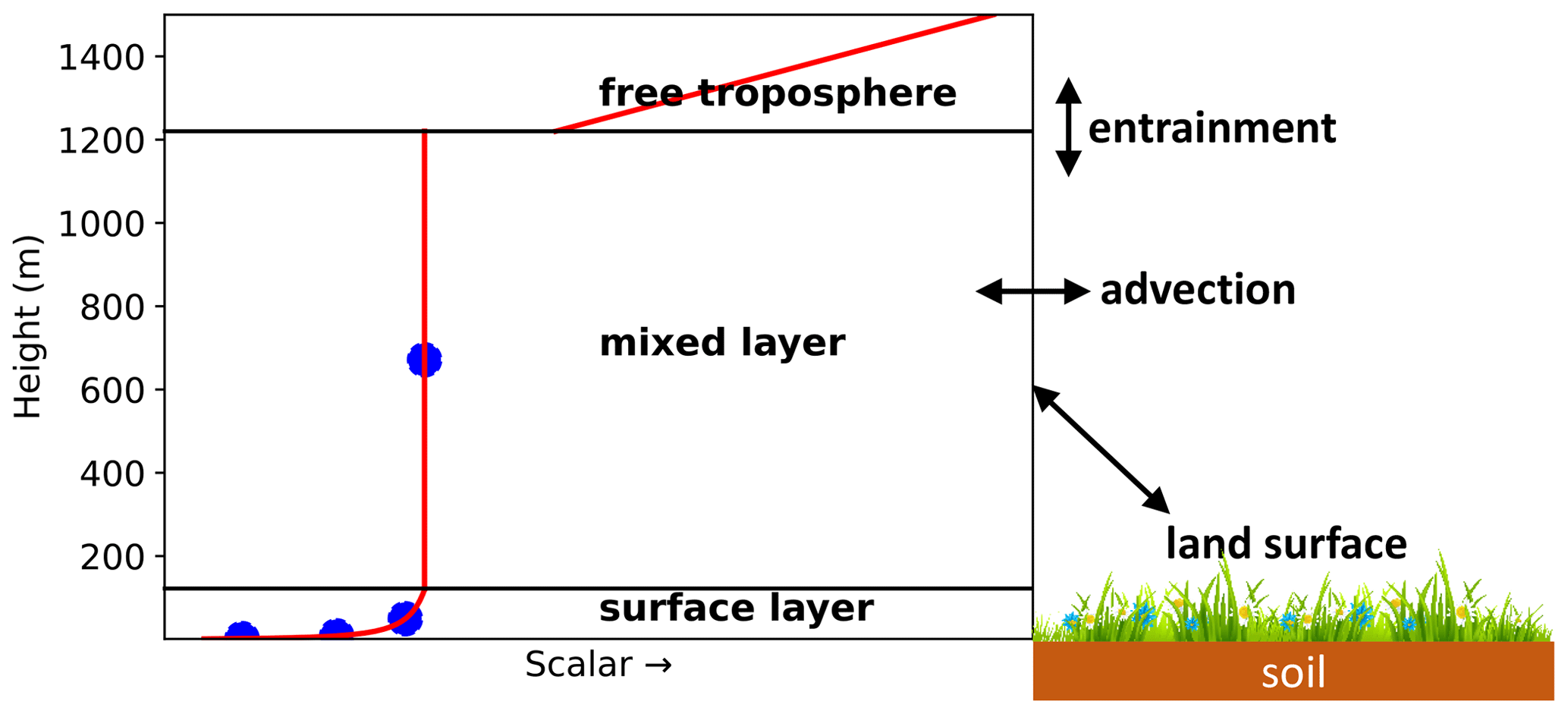
Figure 1Sketch of the employed forward model (the slightly adapted CLASS model). The blue dots in the surface layer represent user-specified heights, where the model calculates scalars, e.g. the CO2 mixing ratio. The mixed layer is represented by a single bulk value in the model (blue dot in the mixed layer). At the top of the mixed layer, a discontinuity (jump) occurs in the profiles. The free troposphere is not explicitly modelled but is taken into account for the exchange with the mixed layer (entrainment). The slope of the free troposphere line is the free tropospheric lapse rate. A constant advection can be taken into account as a source/sink.
3.1 General
Inverse modelling is based on using observations and, ideally, prior information to statistically optimise a set of variables driving a physical system (Brasseur and Jacob, 2017). The n variables to be optimised are contained in a state vector x. In our framework, this vector can be subdivided in two vectors. Those are xm, containing state variables belonging to the input of CLASS (e.g. CO2 advection and albedo), and xb, containing state variables belonging to our bias correction scheme (see Sect. 3.2). The forward-model H (CLASS) projects the vector xm to provide model output that can be compared to observations, e.g. temperatures at different heights (full list in the ICLASS manual). This output does not only depend on xm but also on model parameters that are not part of the state. Those are contained in a vector p. The result is contained in vector H(xm,p). Note that an overview of all inverse-modelling variables defined in this section is given in Table B1, including the dimensions and units. We initially define a cost function J (–) as follows (Brasseur and Jacob, 2017):
where xA represents the a priori estimate of the state vector, y is the vector of observations used within the modelled time window, and H(xm,p) is the vector of model results at the times of the observations. The latter vector is the model equivalent of the observation vector y. The superscript T means transpose, SA represents the a priori error covariance matrix (defined in the Supplement), and SO represents the matrix of the observational error covariances. This cost function quantifies two aspects, namely the fit between model output and observations, in addition to how well the posterior state matches with prior information about the state. Regarding the observational error covariance matrix SO (fully defined in Brasseur and Jacob, 2017), we assume, for simplicity, the observational errors to be uncorrelated (as in, e.g., McNorton et al., 2018; Chevallier et al., 2010; Ma et al., 2021). This simplifies the matrix SO to a diagonal matrix, with the observational error variances as diagonal elements. In this way, Eq. (2) simplifies to the following:
Here, is the ith diagonal element of SO, and m is the number of observations. It is customary to refer to the first term of this cost function as the background part and to the second part of this function as the data part. Note that if the a priori errors are also uncorrelated, then the first term in the equation can be simplified in a similar way as the second term. The observational error variance linked to the ith observation () can be further split up as follows:
where is the instrument (measurement) error variance, is the model error variance, and is the representation error variance (see Brasseur and Jacob, 2017). These errors are assumed to be independent of each other and normally distributed.
At this point, we introduce two extra features to the cost function. First, we allow the user to specify a weight for each individual observation, in case some observations are deemed less important than others. In principle, the observational error variances could also be adapted for this purpose, but, by using weights, we can keep realistic error estimations (important for Sect. 4.2). Those weights can also be used to manipulate the relative importance of the background term and the data term. This is similar to the regularisation factor explained in Brasseur and Jacob (2017). Second, we introduce part of our bias correction scheme in the data part of the cost function, namely scaling factors for observations. These factors can also be optimised. With the additions mentioned above, the cost function, as given in Eq. (3), modifies to the following:
where wi (–) is a weight for each individual observation in the cost function. si (–) is a scaling factor for observation yi, which is identical for each time step but is allowed to differ between each observation stream. The background term in the cost function can be left out if the user desires so. The introduction of the scaling factors means we need to adapt the observational error variances as well. Thus, the ith observational error variance is now given by the following:
where is the unknown vector of the “true” values of the model parameters in the state vector, and is the true value of the scaling factor for the ith observation. The decomposition from Eq. (4) remains valid.

Figure 2Slightly simplified sketch of the workflow of the inverse modelling framework when using the adjoint model for the derivatives with respect to model parameters. Note that, for the purposes of clarity, direct arrows between the parameters and the cost function and its gradients are not drawn. These arrows arise via the background part of the cost function (see the equations in the text). Everything within the shaded rectangle is part of the iterative cycle of optimisation. Model parameters that are not optimised are in the vector p. This vector is used together with xm in every model simulation. In case ICLASS is run in Monte Carlo mode (Sects. 3.6 and 4.2), this figure applies to the individual ensemble members.
In the statistical optimisation, we attempt to find the values of the state vector x, such that the function in Eq. (5) reaches its absolute minimum. This is done by starting from an initial guess (x=xA), after which the state vector is improved iteratively. The cost function and the gradient of the cost function (derivatives with respect to all parameters) are computed for different combinations of parameters in the state vector (Fig. 2). The framework uses, by default, a truncated Newton method, the tnc algorithm (The SciPy community, 2022; Nash, 2000), for the optimisations. Truncated Newton methods are suitable for non-linear optimisation problems (Nash, 2000). The chosen algorithm allows the specification of hard bounds for the state vector parameters, thus preventing unphysical parameter values for individual parameters in the state vector. Raoult et al. (2016) used similar constraints in their inverse modelling system, and Bastrikov et al. (2018) used bound constraints as well. The analytical cost function gradient calculations are described in Sect. 3.4. A basic numerical derivative option (Sect. 3.5) is available as well, although we expect this, in general, to be outperformed by the analytical derivative.
3.2 State vector parameters
As mentioned before, the state vector can be decomposed into vector xm and vector xb. Vector xm contains state variables related to the input of CLASS, such as the initial conditions (e.g. initial mixed layer potential temperature), boundary conditions (e.g. CO2 advection), and uncertain model constants (e.g. roughness length for heat). The full list of model parameters that can be optimised is given in the ICLASS manual.
Vector xb contains parameters belonging to our bias correction scheme in the data part of the cost function. There are two ways of bias correcting. The first one is by using observation scaling factors for observation streams. These scaling factors (si) have been introduced in Eq. (5). As an example, in the state vector to be optimised, one can include a single scaling factor for all CO2 surface flux observations. The second possible method of bias correcting (Sect. 3.3) is implemented specifically for the energy balance closure problem (Foken, 2008; Oncley et al., 2007; Renner et al., 2019), and it involves a parameter FracH (–) to be optimised.
3.3 Bias correction for energy balance closure
We first define an observational energy balance closure residual as follows (Foken, 2008):
where Rn is the time series of net radiation measurements, Horig and LEorig are the measured sensible and latent heat fluxes, and G is the measured soil heat flux. The difference between the measured net radiation and the sum of the measured heat fluxes is calculated for every time step, and this represents the energy balance closure residual. If desired, the user can easily specify an expression of their own for εeb. Subsequently, the observations for the sensible and latent heat flux are adapted as follows:
This implies that the energy balance closure residual is added partly to the sensible heat flux and partly to the latent heat flux, thereby closing the energy balance in the observations. This partitioning is determined by parameter FracH, which is taken to be constant during the modelled period. This approach of closing the energy balance is similar to Renner et al. (2019), but we optimise a parameter, instead of using the evaporative fraction, for partitioning εeb. The limitations of this approach are that we assume the radiation and soil heat flux measurements to be bias-free and the FracH parameter constant.
3.4 Analytical derivative
For the optimisations, we do not only compute a cost function, but we also use the gradient of the cost function with respect to the state vector elements. This informs us on the direction in which the cost function lowers. How the gradient with respect to an individual element is calculated depends on which state vector element is considered. In case the ith state vector element is a model input parameter, the gradient with respect to this element is computed as follows (similar to Brasseur and Jacob, 2017, their Eq. 11.105):
where is the local Jacobian matrix of H. l is the number of non-model-input parameters in the state x occurring before xi. F is the forcing vector, with elements Fk defined as follows:
There is one forcing element in the vector for every observation that is used, and Fk is the forcing related to the observation yk. For calculating the model input part of the analytical derivative, we constructed the adjoint of the model, , which is used to obtain a locally exact analytical gradient (in specific cases the gradient is not exact; see the section of “if statements” in the Supplement). More information on the adjoint is given in the Supplement.
In case the ith state vector element is an observation scaling factor (Eq. 5) for observation stream j, the gradient of the cost function with respect to the ith state vector element is computed as follows:
where mj is the number of observations of the type (stream) to which the observation scaling factor is applied, e.g. if the observation scale is a scaling factor for surface CO2 flux observations, then mj is the number of surface CO2 flux observations. yj,k is the kth observation of this observation stream. Fk is the forcing related to the observation yj,k.
Finally, if the ith state vector element is FracH, then the gradient is calculated as follows:
where FH and FLE are the forcing vectors for the sensible and latent heat fluxes, respectively, yH and yLE are the observation vectors for the sensible and latent heat fluxes, respectively, and ⋅ is the Euclidian inner product. Note that, when the FracH parameter is included in the state, the observation scaling factors for sensible and latent heat flux observations will be set equal to 1 and are not allowed to be included in the state. The terms and represent, respectively, the derivatives of the sensible and latent heat flux observations to the FracH parameter, which follow from Eqs. (8) and (9) as follows:
Note that Eqs. (10), (12), and (13) all have the same first term that originates from the background part of the cost function.
3.5 Numerical derivative
A simple numerical derivative is available as alternative to the analytical gradient. The derivative of the cost function to the ith state element is numerically calculated as follows:
where α is a very small perturbation to state parameter xi, with a default value of 10−6, and has the units of xi.
3.6 Handling convergence challenges
The highly non-linear nature of the optimisation problem can cause the optimisation to become stuck in a local minimum of the cost function (Santaren et al., 2014; Bastrikov et al., 2018; Ziehn et al., 2012). This means that the resulting posterior state vector can depend on the prior starting point (Raoult et al., 2016), and the resulting posterior state can remain far from optimal. In the worst case, the non-linearity of the model can even lead to a crash of the forward model. This happens with certain combinations of input parameters that lead to unphysical situations or undesired numerical behaviour. After starting from a user-specified prior state vector, the tnc algorithm autonomously decides which parameter values are tested during the rest of the optimisation. It is possible to place hard bounds on individual parameters when using the tnc algorithm, but this does not always prevent all possible problematic combinations of parameters from being evaluated.
To obtain information about the uncertainty in the posterior solution, and to deal with the challenges described above, the framework also allows a Monte Carlo approach (Tarantola, 2005). This entails the framework not starting at a single state vector with prior estimates but instead using an ensemble of prior state vectors xA, thus leading to an ensemble of posterior parameter estimates. The ensemble of optimisations can be executed in parallel on multiple processors, thereby reducing the time it takes to perform the total optimisation. More details on the Monte Carlo mode of ICLASS are given in the Sect. 4.2.
As an additional way to improve the posterior solution, we have implemented a restart algorithm. If the optimisation results in a cost function that is higher than a user-specified number, then the framework will restart the optimisation from the best state reached so far. This fresh start of the tnc algorithm, whereby the algorithm's memory is cleared, often leads to a further lowering of the cost function. The maximum number of restarts (>=0) is specified by the user. If an ensemble is used, then every individual member with too high a posterior cost function will be restarted.
4.1 Prior and observations
From a Bayesian point of view, ICLASS can combine information, both from observations and from prior knowledge about the state vector, to come to a solution with a reduced uncertainty in the state parameters. In the derivation of Eq. (2), it is assumed that both prior and observational errors follow a (multivariate) normal distribution (Tarantola, 2005). However, some prior input parameters are bounded (Sect. 3.6), e.g. the albedo cannot be negative. Dealing with bounds is a known challenge in inverse modelling, and several approaches can be followed (Miller et al., 2014). As an example, Bergamaschi et al. (2009) had to deal with methane emissions in the state vector becoming negative. Their solution was to make the emissions a function of an emission parameter that is being optimised instead of optimising the emissions themselves. Through their choice of function, the emissions cannot become negative, even though the emission parameter is unbounded. In our case, such an approach is more difficult, as we have a diverse set of bounded parameters.
Our approach is to enforce hard bounds for state values via the tnc algorithm. It, however, means that the normality assumption will be violated to some extent, as the normal distribution (for which the user specifies the variance) for prior parameter values then becomes a truncated normal distribution. For a parameter following a truncated normal prior distribution, the prior variance used in the cost function is not (fully) equal to the variance of the actual prior distribution. The extent to which this is the case depends on the degree of truncation.
Our system also allows for specifying covariances between state elements in SA. We assume observational errors to be uncorrelated (see Sect. 3.1). Equation (4) states that the observational error variance consists of an instrument error, a model error, and a representation error variance. The instrument and representation error standard deviation are taken from user input, while the model error standard deviation can either be specified by the user or estimated from a sensitivity analysis. In the latter case, an ensemble of forward-model runs is performed. For each of these runs, a set of parameters, not belonging to the state vector, is perturbed (so the parameters are part of the vector p and not from xm; see Sect. 3.1). These perturbed parameters are used together with the unperturbed prior vector xm as model input. The user should specify which parameters should be perturbed, and the distribution from which random numbers will be sampled to add to the default (prior) model parameters. For the latter, there is the choice between a normal, bounded normal, uniform, or triangular distribution. The model error standard deviation for each observation stream at each observation time is then obtained from the spread in the ensemble of model output for the observation stream at that time.
4.2 Ensemble mode to estimate posterior uncertainty
When ICLASS is run in Monte Carlo (ensemble) mode, it allows the estimation of the uncertainty in the posterior state. The principle for obtaining posterior error statistics bears a strong similarity to what has been done in Chevallier et al. (2007), and our method will be shortly explained here. We start with the prior state specified by the user. Then, for each ensemble member and for every state parameter, a random number is drawn from a normal distribution with the variance of the respective parameter specified by the user and a mean of 0. When covariances are also specified for the prior parameters, a multivariate normal distribution can be used to sample from. The sampled numbers are then added to the state vector. In case any non-zero covariances are used to perturb, and then, if the new state vector falls out of bounds (if specified), it is discarded, and the procedure is repeated for that ensemble member. In case no covariance structure is used, then only the parameter which falls out of its bounds has to be replaced. It has to be noted that this effectively leads to sampling from a truncated (multivariate) normal distribution.
Similarly, for every ensemble member, a random number drawn from a normal distribution (without bounds) is added to the (scaled) observations. This modifies the cost function of an individual ensemble member (Eq. 5) as follows:
is the perturbed prior state vector. The random numbers εi in the data part of the cost function are sampled from normal distributions with mean 0 and standard deviation σO,i. This can be seen as either a perturbation of the scaled observations or a perturbation of the model–data mismatch. As a consequence of the change in the cost function equation, the equation for the forcing vector (Eq. 11) is updated as well:
Furthermore, in Eqs. (10), (12), and (13), for perturbed ensemble members, is used instead of xA. The vector εeb (Eq. 7) is not perturbed and kept identical for all members. For every ensemble member, an optimisation is performed. Each optimisation is classified as being either successful or not successful. Here, “successful” is defined as having a final reduced chi-square (see Sect. 5; Eq. 19) smaller or equal than a user-specified number. The posterior state parameters for the successful members are considered a sample of the posterior state space and are saved in a matrix. Those parameters can be used to estimate the true posterior probability density functions (pdf's). A covariance and a correlation matrix are then constructed using the matrix of the posterior state parameters. These covariance and correlation matrices are used as an estimate of the true posterior state covariance and correlation matrices, respectively. If the user prefers to do so, the numeric parameters not belonging to the state can also be perturbed in the ensemble, in a similar way to that outlined in Sect. 4.1.
Note that, next to the ensemble, there will also be a run with an unperturbed prior, just as is the case when no ensemble is used. We refer to this run as member 0. This member is, however, not included in the calculation of ensemble-based error statistics (e.g. correlation matrix), as the choice of prior values is not random for this member.
ICLASS can write several output files. The output includes the obtained parameters, the posterior reduced chi-square statistic, and the posterior and prior cost function. The reduced chi-square goodness-of-fit statistic is defined in ICLASS as follows:
In this equation, m is the number of observations, and n is the number of state parameters (see Sect. 3 for the other symbols). Note that if all the weights are set to 1, then the denominator simplifies to m+n. The n will only be included in the denominator when the user chooses to include a background part in the cost function (default). In a simple case where the prior errors are uncorrelated, this statistic for the posterior solution should be around 1 when the optimisation converges well and priors and errors are properly specified (e.g. Michalak et al., 2005). In a case where all weights are 1, this can be understood as follows. The average value of the ith posterior observation residual squared, , should be close to , and the average value of the ith posterior data residual squared, , should be close to the ith diagonal element of the a priori error covariance matrix when the optimisation converges well and errors and prior parameters are properly specified. We have m observation residuals and n data residuals (if background part included). In this example with a diagonal SA matrix, the residuals are assumed to be independent of each other. Each squared residual contributes on average a value of approximately 1 to the cost function, summing to approximately m+n and, thus, . Note, however, that the statistic can be misleading, in particular when observational errors are correlated (Chevallier, 2007). Furthermore, as mentioned in Sect. 4.1, prior parameters can follow a truncated normal distribution, violating the normality assumption. The impact of this depends on the degree of truncation and also on the number of observations and so on. It can lead to an ideal value diverting from 1.
ICLASS also calculates a prior and posterior partial cost function and a posterior statistic for individual observation streams and for the correspondence to prior information (background). The partial cost function for observation stream j is calculated as follows:
where mj is the number of observations of stream j, yj,i is the ith observation of stream j, and H(xm,p)i is the model output corresponding with yj,i. In case scaled observations are perturbed in the ensemble (Sect. 4.2), εi is a random number; otherwise, it is 0. The statistic for observation stream j is defined here as follows:
This equation resembles Eq. (13) in Meirink et al. (2008), but note that the variable in their paper is similar to in our paper. The statistic for the background part is calculated as follows (similar to Eq. 26 of Michalak et al., 2005):
where Jb is the background part of the cost function, i.e. the first term from Eq. (5). The mean bias error, root mean squared error, and the ratio of model and observation variance for every observation stream is also calculated, both for the prior and posterior state. The mean bias error for the jth observation stream is defined here as follows:
In this equation, mj is the number of observations of type (stream) j, is the model output for observation stream j at time index i, yj,i is an observation of stream j at time index i, and sj is an observation scaling factor for observations of stream j. Note that, even when the scaled observations are perturbed, we do not include those perturbations here (compare Eq. 20). In case the FracH parameter is used, the energy-balance-corrected observations (Eqs. 8 and 9) will be used in the equation above. For the root mean squared error and the ratio of model and observation variance, the observation scales and energy-balance-corrected observations are used as well. ICLASS also calculates the normalised deviation of the posterior from the prior for every state parameter xi as follows:
where σA,i is the square root of the prior variance of parameter i, i.e. the square root of diagonal element i from matrix SA. Note that, also in case of an ensemble, we use the unperturbed prior, i.e. the prior of member 0.
If run in ensemble mode, we additionally store estimates of the posterior error covariance matrix (Sect. 4), the posterior error correlation matrix, the ratio of the posterior and prior variance for each of the state parameters, the mean posterior state, and the optimised and prior states for every single ensemble member. When non-state parameters are perturbed in the ensemble, these parameters are part of the output. Moreover, the correlation of the posterior state parameters with these non-state parameters can also be written as output. When the model error standard deviations are estimated by ICLASS (Sect. 4.1), there is a separate file containing statistics on the estimated error standard deviations. Finally, there are additional output files with information about the optimisation process. For every model simulation (and for every ensemble member) in the iterative optimisation process, one can find the parameter values used in this simulation and the value of the cost function split up into a data and a background part. For the gradient calculations, one can find the parameter values used and the derivatives of the cost function with respect to every state parameter. The derivatives of the background part are also provided separately. More details on the output of ICLASS can be found in a separate section of the manual. An overview of the output variables defined in this section is given in Table B2.
We have written the entire code in Python 3 (https://www.python.org, last access: 9 December 2022). Using the framework requires a Python 3 installation, including the NumPy (van der Walt et al., 2011; https://numpy.org), SciPy (https://scipy.org, last access: 9 December 2022), and Matplotlib (Hunter, 2007; https://matplotlib.org, last access: 9 December 2022) libraries. The code is operating system independent and consists of the following three main files:
-
forwardmodel.py, which contains the adapted CLASS model.
-
inverse_modelling.py, which contains most of the inverse modelling framework, such as the function to be minimised in the optimisation and the model adjoint.
-
optimisation.py, which is the file to be run by the user for performing an actual optimisation. In this file, the observations are loaded, the state vector defined, and so on. The input paragraphs in this file should be adapted by the user to the optimisation performed.
There are three additional files. The first is optimisation_OSSE.py and is similar to optimisation.py but is meant specifically for observation system simulation experiments (also, in this file, the user should adapt the input paragraphs to the optimisation to be performed). The second file is testing.py, which contains tests for the code, as described in Sect. 7. The file postprocessing.py is a script that can be run, after the optimisations are finished, for post-processing the output data, e.g. to plot a coloured matrix of correlations. Using the Pickle module, the optimisation can store variables on the disk near the end of the optimisation, and these variables can be read in again in the postprocessing.py script. This has the advantage that, for example, the formatting of plots can easily be adapted without redoing the optimisation. This script should be adapted by the user to the optimisation performed and the output desired.
When using the adjoint modelling technique, an extensive testing system is required to make sure that the analytical gradient of the cost function computed by the adjoint model is correct. There are two tests that are essential, which are described below.
The gradient test (for the tangent linear model) is a test to determine whether the derivatives with respect to the model input parameters in the tangent linear model are constructed correctly. The construction of the adjoint is based on the tangent linear model, so errors in the tangent linear propagate to the adjoint model. In the gradient test, model input state variables are perturbed, leading to a change in model output. The change in model output when employing the tangent linear model is compared to the change in model output when a numerical finite difference approximation is employed. Mathematically, the test for the ith model output element can be written as follows (similar to Honnorat et al., 2007; Elizondo et al., 2000):
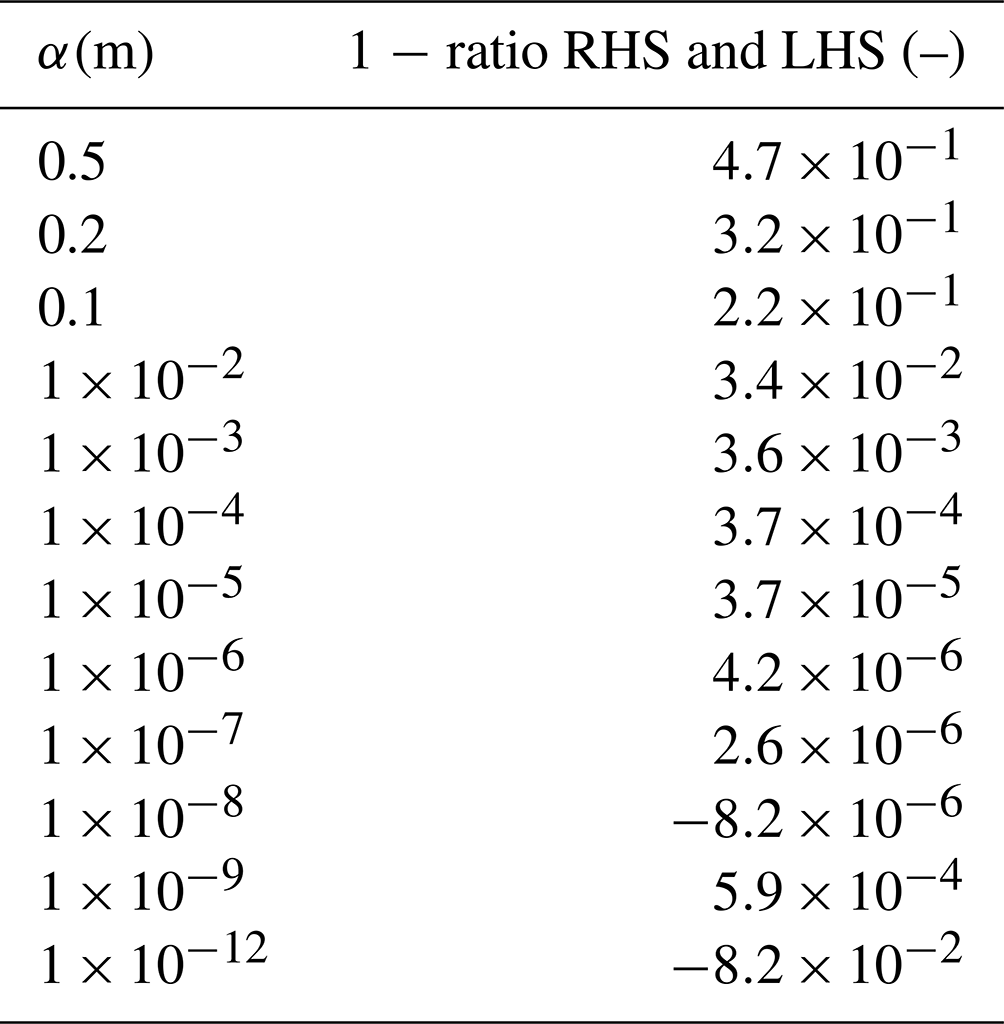
where Δxm is a vector of ones, with the same length as vector xm. α is a small positive number, H represents the forward-model operator, H(xm,p)i is the ith model output element, xm is the vector of the model input variables to be tested (model parameters part of state), ⋅ is the Euclidian inner product, and vector p is the set of non-state parameters used by the model. Several increasingly smaller values are tested for α. When the tangent linear model is correct, then the right-hand side of the equation will converge to the left-hand side when α becomes progressively smaller, although for too small α values, numerical errors start to arise (Elizondo et al., 2000). Instead of using the full tangent linear model, individual model statements can also be checked. In this case, xm and H(xm,p)i can contain intermediate (not part of model input or output) model variables. The gradient test is considered successful if the ratio of the left- and right-hand sides of the equation lies in the interval [0.999–1.001]. The results of a simple example of a gradient test, involving the derivative of the 2 m temperature with respect to the roughness length for heat (z0h), is shown in Table 1.
Table 1A simple gradient test example involving the derivative of the 2 m temperature with respect to the roughness length for heat (z0h). The right column gives, for different values of perturbation α (m), the result of the calculation 1 − RHS divided by LHS, whereby RHS is the right-hand side of Eq. (25), and LHS is the left-hand side of the same equation. Note that only the RHS of the equation is influenced by α. In this example, we have only perturbed parameter z0h, but multiple parameters can be perturbed within one test.
The dot product (adjoint) test checks whether the adjoint model code is correct for the given tangent linear code. It tests whether the identity
holds (Krol et al., 2008; Meirink et al., 2008; Honnorat et al., 2007; Claerbout, 12004). The equation can also be written as follows:
In this equation, represents the tangent linear model operator, i.e. a matrix (the local Jacobian of H) with the element on the ith row and jth column given by . xm is, in this equation, a vector with perturbations to the model state, represents the adjoint model operator, and 〈〉 is the Euclidian inner product. A very small deviation from 0 is acceptable due to machine rounding errors (Claerbout, 12004). Our criterion for passing the test, when using 64 bit floating point calculations, is that the absolute value of the left-hand side of Eq. (27) should be . This test can also be applied to individual statements or a block of statements in the adjoint model code. In this case, the definitions of the variables in Eq. (27) change slightly, e.g. then represents a part of the adjoint model. The adjoint test will be illustrated by a (slightly simplified) example from the model code, namely the well-known Stefan–Boltzmann law for outgoing longwave radiation. The forward-model code reads as follows:
Lwout = bolz * Ts ** 4.
The tangent linear model code for this statement reads as follows:
dLwout = bolz * 4 * Ts ** 3. * dTs.
And the corresponding adjoint code is as follows:
adTs += bolz * 4 * Ts ** 3. * adLwout
adLwout = 0.
In this case, xm corresponds to dTs, and the HLxm variable is dLwout. The vector y is adLwout, and is adTs. In the test, xm and y are assigned random numbers. When we evaluated Eq. (27) on this part of the code, the result was less than (which corresponds to approximately 5 × the machine precision), meaning that the test passes.
We have constructed a separate script that performs a vast number of gradient tests and adjoint tests and informs the user whenever a test fails. This file (testing.py) is included with the code files. The number of time steps we specified for testing is small, as the computational burden increases with the number of time steps. The model passes the vast majority of the tests that are executed in this file. Closer inspection of the tests that fail reveals that numerical noise is a likely explanation for the small fraction of tests that are labelled as failing. Further validation of the inverse modelling framework follows in the next section.
To test the ability of the system to properly estimate model parameters, we show, in this chapter, the results of observation system simulation experiments (OSSEs) with artificial data. These types of experiments are classically used to test the ability of the system to properly estimate model parameters. For example, similar tests have been performed by Henze et al. (2007), for their adjoint of a chemical transport model. In our experiments, we simulate a growing convective boundary layer for a location at mid-latitudes from 10–14 h, including surface layer calculations. In the chosen set-up, the land surface is coupled to the boundary layer. The land surface provides heat and moisture and exchanges CO2 with the CBL.
8.1 Parameter estimation
We perform, in this section, a total of five main experiments of varying complexity. The things that differ among experiments are the choice of observations and state vectors. The procedure for the first four experiments is as follows. We first run the model with chosen values of a set of parameters we want to optimise. A set of model output data from this simulation then serves as the observations, while the parameters used to create these observations are referred to as the true parameters. Then we perform an optimisation using these observations, starting from a perturbed prior state vector. In the cost function, we do not include the background part to make sure that it is possible to retrieve the true parameters. This is because the background part of the cost function implies a penalty for deviating from the prior state. This penalty implies that, when the model is run with the true parameters, the cost function would still not be 0. Next to that, the minimum of the cost function is (generally) shifted. When leaving out the background part, the framework should, if converging properly, be able to find back the parameter values that were used for creating the observations, starting from any other prior state vector.
Since real-life observations usually contain noise, the last experiment follows the same procedure, except that the observations are also perturbed. This is done by adding white Gaussian noise to the observations. For each observation yi, a random number drawn from a normal distribution with mean 0 and standard deviation equal to a specified σI,i (Table 3) is added. The model and representation errors are set to 0 in all experiments. All weights for the cost function were set to 1. Table 2 lists, for every experiment, the prior, the true, and the optimised state variables. The complexity of the experimental set-up increases from the top to the bottom of the table.
Table 2Parameter values for the main observation system simulation experiments of Sect. 8.1. The observation streams used in the two obs (observation) streams experiments are q and h, for the six obs streams experiment, H, LE, T2, and are added, and for the seven obs streams experiments, is additionally added. The value of, for example, parameter z0m (only a state element in the 10-parameter-state experiments) is in the 2-parameter-state and 5-parameter-state experiments equal to the true value of z0m in the 10-parameter-state experiments. See Table A1 for a description of the parameters and Table A2 for a description of the observation streams. Note: ppm is parts per million.
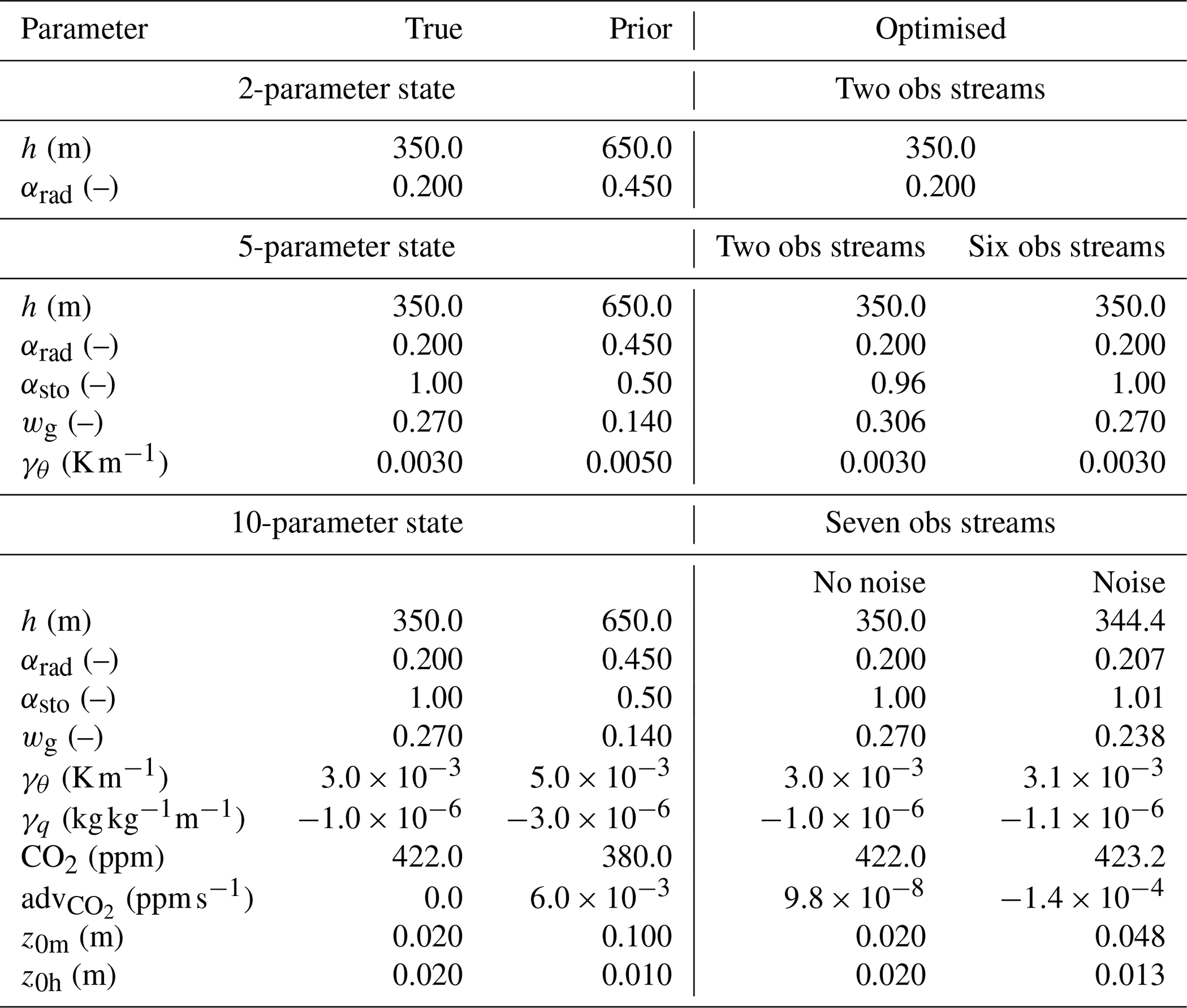
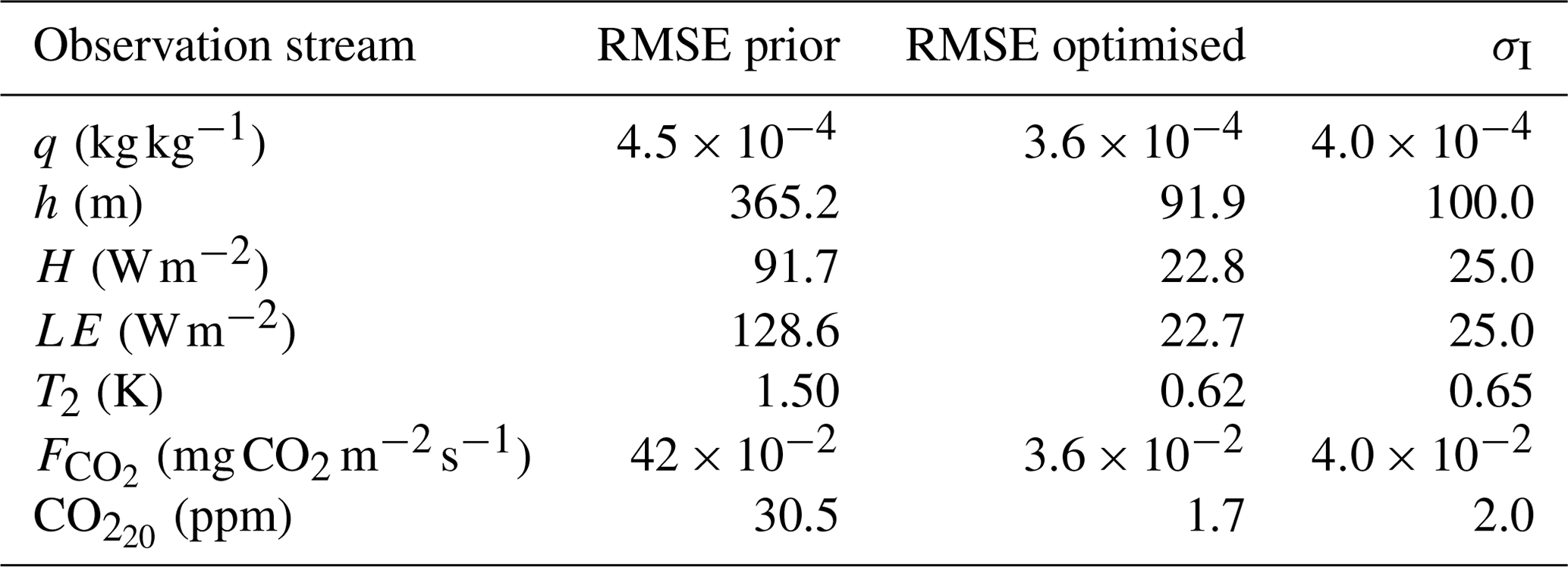
Table 3The root mean squared error (RMSE) and the specified measurement error standard deviation (σI) for the observation streams in the 10-parameter-state OSSE with perturbed observations. In all our OSSEs, the measurement error standard deviations are chosen to be constant with time. Note that the measurement error equals the observational error here, since the model and representation errors were set to 0 for simplicity. The σI are identical for all OSSEs in Table 2, but not all observation streams are used in each OSSE.
For the first experiment, we perturbed the initial boundary layer height and albedo. The rest of the parameters are left unchanged compared to the true parameters. The observation streams we used are specific humidity and boundary layer height. The specific humidity is expected to be influenced by the albedo, as the amount of available net radiation is relevant for the amount of evapotranspiration, which influences the specific humidity. The boundary layer height is relevant for specific humidity as well, as it determines the size of the mixing volume in which evaporated water is distributed. The state parameters are thus expected to have a profound influence on the cost function.
The optimised model shows a very good fit to the observations (Fig. 3), and the original parameter values are found with a precision of at least five decimal places (Table 2; fewer than five decimal places are shown). This result indicates the optimisations work in such simple situations.
To test the system for a more complex problem, we change from two parameters in the state to five (Table 2; second block), while keeping the same observations. Again, based on physical reasoning, the added parameters are expected to influence the cost function. However, one might expect that the observations might not be able to uniquely constrain the state, i.e. parameter interdependency issues might arise for this set-up (equifinality). As an example, a reduction in soil moisture might influence the observations in a similar way as a reduction in stomatal conductance does. Mathematically, this means that multiple nearly equivalent local minima might be present in the cost function.
Also for this more complex case, we manage to obtain a very good fit (Fig. 3c and d). However, inspecting the obtained parameter values (Table 2; second block; column labelled “Two obs streams”), we see that the optimisation does not fully converge to the true state. This is likely caused by parameter interdependency, as described earlier. To solve this, extra observation streams need to be added that allow the disentangling of the effects of the different parameters in the state. We have tested this in the third experiment by adding the sensible and latent heat flux, the temperature at 2 m height, and the surface CO2 flux to the observations. With this more complete set of observations, the true parameter values are found with a precision of at least four decimal places (column labelled “Six obs streams” in Table 2). As a side experiment, not included in Table 2, we have run the same experiment as before but using the numerical derivative described in Sect. 3.5. In this case, convergence is notably slower, e.g. more than 6 times as many iterations were needed to reduce the cost function to less than 0.1 % of its prior value. This indicates that, at least for this more complex non-linear optimisation case, an analytical gradient outperforms our simple numerical gradient calculation.
In the fourth main experiment, we increase the number of state parameters to 10 (Table 2). To further constrain the parameters, we expand our set of observation streams with the CO2 mixing ratio measured at 20 m height. Also, for this complex set-up, the framework managed to find the true values, with a precision of one decimal place for the initial boundary layer height and more for the other parameters.
These tests show that (at least for the range of tests performed) the framework is able to find the minimum of the cost function well. Additionally, we performed another observation system simulation experiment to test the framework's usefulness in a more realistic situation with noise on the observations. The result can be seen in Fig. 3e–h. The framework finds a good fit to the observations, even though it has now become impossible to fit every single (perturbed) observation. The posterior root mean squared error is about the same size (slightly smaller) as the observational error standard deviation for all observation streams (Table 3). This confirms the visual good fit from Fig. 3e–h, given that these observational error standard deviations were used to create the random perturbations for the observations. The statistic of the optimisation has become close to 1 (0.83), indicating no strong over- or under-fitting of the observations.
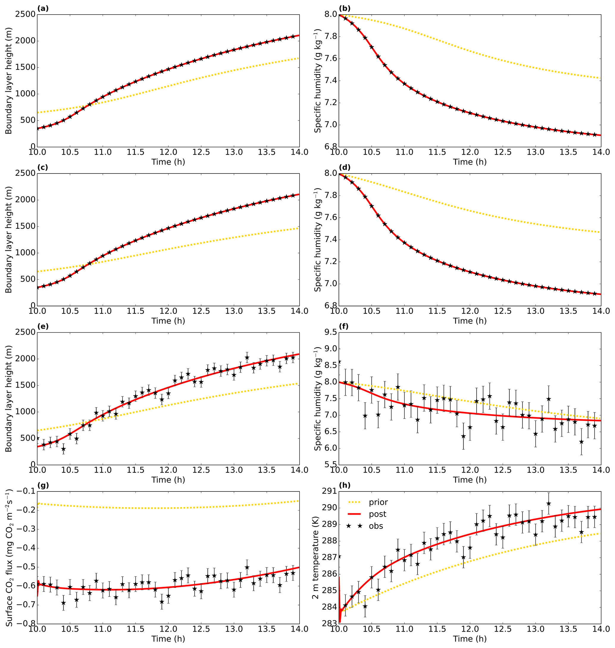
Figure 3Model output from three observation system simulation experiments from Sect. 8.1, namely the two-parameter-state experiment with albedo and the initial boundary layer height (top row), the five-parameter-state experiment with two observation streams (second row), and the experiment with perturbed observations (third and fourth rows). The term “post” means posterior, i.e. the optimised simulation. Even though the posterior lines look very similar for the first and second rows, the model parameters are not identical. The specific humidity is from the mixed layer. The error bars show the observational error standard deviations σO, which are here equal to σI.
8.2 Posterior uncertainties and bias correction
In this section, we describe two additional experiments that focus on the validation of the two bias correction methods (Sect. 3) and the posterior uncertainty in the optimised parameters. As a starting point, we take the 10-parameter-state experiment with unperturbed observations from the previous section. We add two additional state parameters related to bias correction (Table 4). We have tested that, for this set-up, ICLASS is able to retrieve the true parameters well (Table 4; column labelled “Optimised unp.”), including the parameters related to bias correction (FracH and ). We now perturb the true observations by adding, to each observation yi, a random number from a normal distribution with mean 0 and standard deviation 1.5 σO,i. The factor 1.5 means that we misspecify the observational errors in the framework, as can happen in real situations too. In this OSSE, we will not simply attempt to fit the observations as well as possible, but we want to employ both observations and prior information. We therefore include the background part of the cost function. The prior error standard deviations are given in Table 4; the a priori error covariance matrix was chosen to be diagonal. As we want an estimate of the posterior parameter uncertainty, we ran ICLASS using an ensemble of 100 perturbed members. For simplicity, we take the total observational error equal to the measurement error, as for the previous OSSEs.
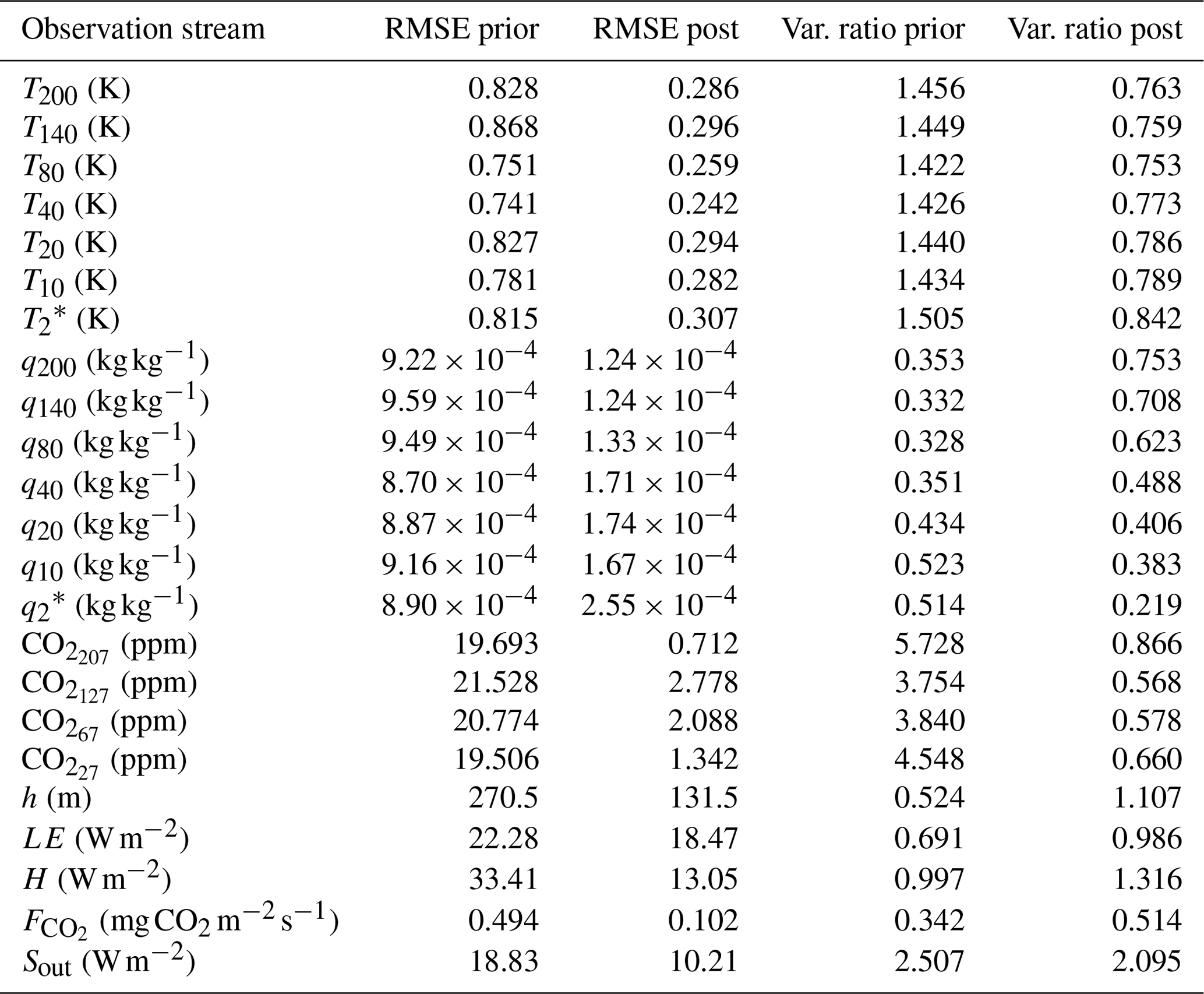
From the 101 members in the ensemble, the unperturbed optimisation has the lowest posterior cost function. Figure 4 indicates that the optimised solution shows a strongly improved fit with the (adapted) observations compared to the prior fit. As expected, due to the perturbations on the observations and the background part of the cost function, the true parameters are not found anymore. For slightly more than half of the state parameters, the optimised parameter value is located less than 1 posterior standard deviation away from the true value (Table 4; rightmost column). The largest relative deviation from the truth is for wg, and the posterior value is approximately 2 standard deviations away from the true value. The parameter uncertainty, as expressed by the standard deviations of the state parameters in Table 4, is reduced for every parameter after the optimisation. In addition, the posterior root mean squared error (RMSE) is reduced for every observation stream after optimisation (Table 5). We see that the posterior RMSE now approaches 1.5×σO, which can be explained by the intentional misspecification of errors. For the same reason, the values of the partial reduced chi-square statistics () should be near 2.25 (1.5 × 1.5) for all observation streams, except CO. The latter is more complex due to the presence of the bias correction scaling factor (). Indeed, we find values ranging between 2.09 and 2.17 for all streams, except CO (Table 5). Note that, for the analysis of the posterior uncertainty, we have only used members with a posterior equal to or lower than 4.5. Therefore, only 38 of the 100 perturbed members were used. We conclude here that ICLASS performs well in all our tests with artificial data, and we present an application with real observations in the next section (more extensive).
Table 4Parameter values for the bias correction OSSEs. The used observation streams are q, h, H, LE, T2, , and CO. σA and σpost are, respectively, the prior and posterior standard deviation of the state parameters. The rightmost column lists the optimised parameter value minus the true value, normalised with the posterior standard deviation of the respective parameter. The column Optimised unp. lists the optimised parameter values of the experiment without any perturbed observations. The four columns at the right-hand side only apply to the OSSE with perturbed observations. See Table A1 for a description of the parameters and Table A2 for a description of the observation streams.

Table 5The prior and posterior root mean squared error (RMSE), the specified measurement error standard deviation (σI), and the partial reduced chi-square statistic () for the observation streams in the bias correction OSSE with perturbed observations. The RMSE and values are for the member with the lowest posterior cost function, i.e. the member with unperturbed prior. Note that the measurement error equals the observational error here, since the model and representation errors were set to 0 for simplicity. All weights for the cost function were set to 1. We used a total of 280 individual (artificial) observations in the cost function. See Table A2 for a description of the observation streams.
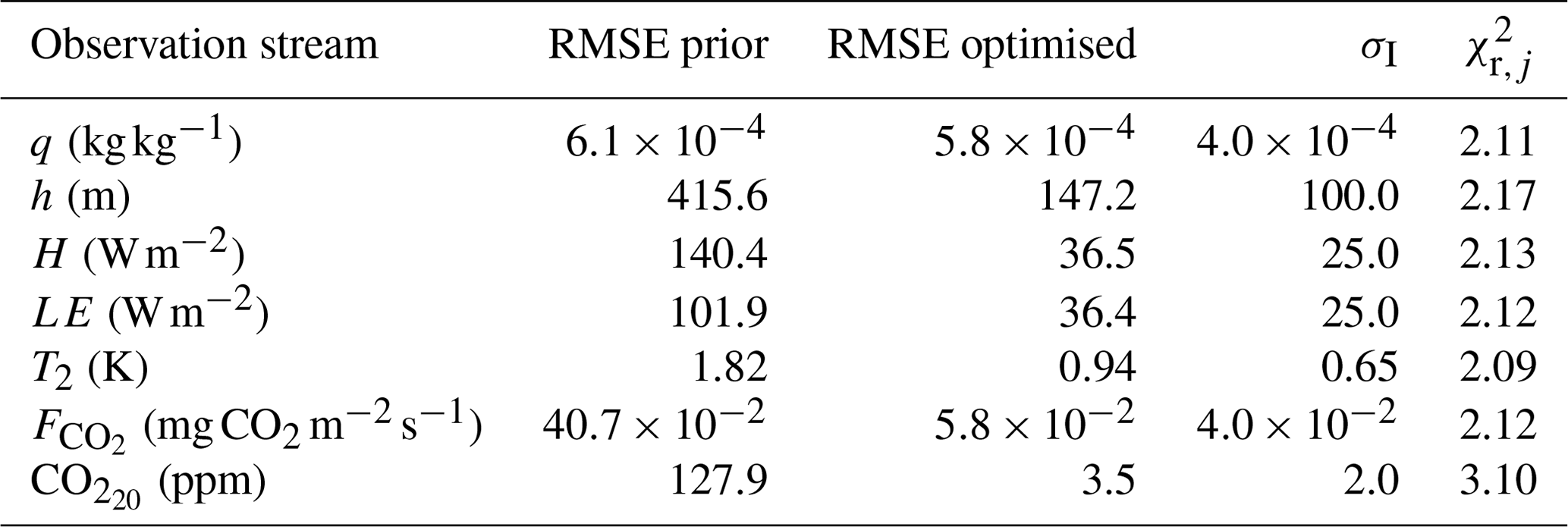

Figure 4Model output and observations for the bias correction OSSE with perturbed observations. The full red line shows the optimised model (“post” means posterior), and the dashed yellow line is the prior model. The (uncorrected) observations are shown by a black star. The error bars show the measurement error standard deviation σI (here equal to σO) on the observations. In panel (b), the red-filled circles are the scaled observations, i.e. . In panels (c) and (d), the black stars are the original (although perturbed) observations, and the red dots are the observations after applying Eqs. (8) and (9).
9.1 Set-up
For this example of how the framework can be used, we used data obtained at Cabauw, the Netherlands, from 25 September 2003. A 213 m high measurement tower is present at this location (Bosveld et al., 2020). This day is chosen here since it has been used in several studies before (Vilà-Guerau De Arellano et al., 2012; Casso-Torralba et al., 2008), and we consider it to be a golden day (Sect. 1), for which the CLASS model is expected to perform at its best.
The set of observation streams we used is given in Table 6, and a description of these streams is given in Table A2. Some of the observations we used are not directly part of the Cabauw dataset; we have derived them from other observations in the same dataset. The parameters we optimise (the state) are given in Table 7, and a description of these parameters can be found in Table A1. The model settings, prior state, and non-state parameters are to a large extent based on Vilà-Guerau De Arellano et al. (2012). The modelled period is from 09:00–15:00 UTC, and we activated the surface layer option in the model. We ran ICLASS in the ensemble mode with 175 members, and an ensemble member was considered successful when having a final (Eq. 19). The prior error standard deviations are given in Table 7. The a priori error covariance matrix was assumed to be diagonal. The representation errors were set to 0. The chosen weights and model and measurement error standard deviations are given in the supplementary material, and further detailed settings of the optimisation can be found via the Zenodo link in the code and data availability section.
9.2 Computational costs
To give an idea of the computational costs involved, we added a timer to an optimisation. An optimisation, like the one described in this section but without the use of an ensemble, took, in our specific case, about 1000 times the time of an individual model simulation using the original CLASS model. However, in our test, an individual simulation with this model took less than 1 s using a single CPU, so the computational cost is still relatively small. The total time it takes to perform an optimisation is dependent on how well the optimisation converges and on the configuration. Using an ensemble increases the computational costs, but multiple ensemble members can be run in parallel on multiprocessor computing systems. An optimisation with an ensemble, like the one described in this section, took, in our specific case, approximately 2 h, using 32 cores of a high-performance computing cluster. The total summed CPU time was about 45 h.
9.3 Model fit
Figure 5 shows that the optimised run shows a much better fit than the prior run to the subset of observations present in this figure. For temperature, a total of seven observation heights are included, but we only show three for brevity. The cost function is reduced from 4702 to 126. The goodness-of-fit statistic has a value of 0.80 for the optimised run, indicating a slight overfitting (or non-optimal error specifications). For all observation streams, the root mean squared error (Sect. 5; Table 6) and the absolute value of the mean bias error (Eq. 23; not shown) are reduced after optimisation. The ratio of model and observation variance becomes closer to 1 for the vast majority of observation streams, except for three of the specific humidity streams and the sensible heat flux.
9.4 Bias correction
Let us now turn to the energy balance (Fig. 6). As described in Sect. 3.3, we forced the energy balance in the observations to close by partitioning the energy balance gap partly to H and partly to LE. From Fig. 6, it is clear that, in the original observations, the sum of H and LE is generally lower than in both the prior and posterior model runs. Both the model and the corrected observations take the energy balance into account. When the difference in Rn−G between model and observations is small (Eq. 7), we might normally expect the model to more easily fit the corrected observations than the original ones. Also in this example, the posterior fit is improved compared to the prior, especially for the sensible heat flux (Table 6). We notice that most of the additional energy is partitioned to LE (Table 7 and Fig. 6). The energy balance closure residual (LHS of Eq. 7) is important to account for in this case, as the mean value of the residuals is only 11 % smaller as the mean of the measured (without applying Eq. 8) sensible heat flux. Note that, for some of the data points around noon, the energy balance correction tends to decrease the heat fluxes (Fig. 6). Inspection of a satellite image of that day revealed that this is likely caused by the presence of high clouds, causing a fast drop in net radiation. The measured heat fluxes tend to react slower, however, leading to a negative value for some elements of vector εeb in Eq. (7).
As is the case for the surface energy balance closure problem, there can also be biases in the CO2 flux eddy covariance observations (Liu et al., 2006). Here we have neglected this for simplicity.
Table 6Observation fit statistics for the Cabauw optimisation. The left columns show the root mean squared error (RMSE) for the prior and posterior state. The two right columns show the ratio between the model and observation variance for the prior and posterior state. Only model data points for times at which we have an observation available are taken into account. We used a total of 670 individual observations in the cost function. The chosen cost function weights and model and measurement error standard deviations are given in the Supplement. The sensible and latent heat flux observations used are corrected for the energy balance gap (see Eqs. 8 and 9). The observation streams are described in Table A2.
* The 2 m temperature and 2 m dew point observations (the latter used for deriving q2) were actually taken at 1.5 m. We do our calculations as if the observations were taken at 2 m. This rounding might have introduced some bias to the T2 and q2 observations. We tested the impact of this by performing a corrected optimisation (without an ensemble). The state parameters resulting from this optimisation were all within the 2 standard deviation posterior uncertainty range of the uncorrected optimisation (x±2σpost), and 9 out of 14 parameters were within the 1 standard deviation uncertainty range (x±σpost).
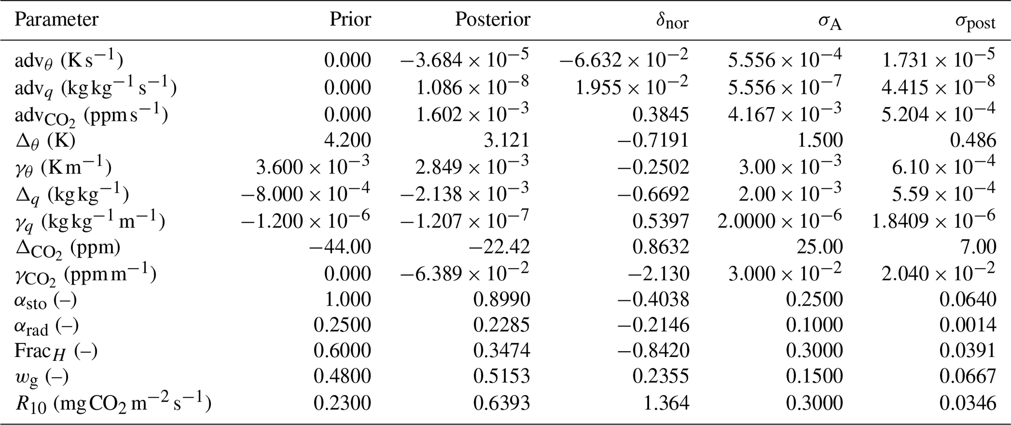
Table 7State parameters for the Cabauw optimisation. δnor is the normalised deviation, i.e. the posterior minus the prior, normalised with the square root of the prior variance (Eq. 24). σA and σpost are, respectively, the prior and posterior standard deviation of the state parameters.
9.5 Optimised parameters
The optimised state is shown in Table 7. Advection of heat remains relatively close to 0 after optimisation (−0.13 ± 0.06 K h−1, where 0.06 is σpost). This is slightly outside the range of 0.1–0.3 K h−1 found by Casso-Torralba et al. (2008), who analysed the same day (using a longer time period). The result can be considered to be in agreement with Bosveld et al. (2004), who concluded large-scale heat advection to be negligible for this day. For CO2, however, we find an advection of 5.8 ± 1.9 ppm h−1 (where ppm is parts per million), which is higher than what was found by Casso-Torralba et al. (2008, their Fig. 9). We shortly return to this in Sect. 9.6. The two parameters that deviate the most from their prior values (normalised with the prior standard deviation; Table 7) are and R10. Both parameters are linked to the CO2 budget, influences the amount of entrained CO2 from the free troposphere, while R10 influences the amount of CO2 entering the mixed layer via respiration. From Fig. 5c, it is clear that the prior run has way too strong a net surface CO2 flux compared to the observations, which explains why R10 is strongly increased in the optimised state. Two main pathways through which the CO2 flux can decrease (in magnitude) are either by increasing R10 or by decreasing the conductance (via αsto). However, the latter also impacts the model fit of the latent heat flux. Unfortunately, separate measurements of gross primary production (GPP) and respiration (e.g. derived from carbonyl sulfide observations; Whelan et al., 2018) are not available in our dataset. These could help to further constrain the CO2-related parameters. In a more detailed study, the parameter estimates might still be improved by, for example, better estimating the vector p and the observational errors.
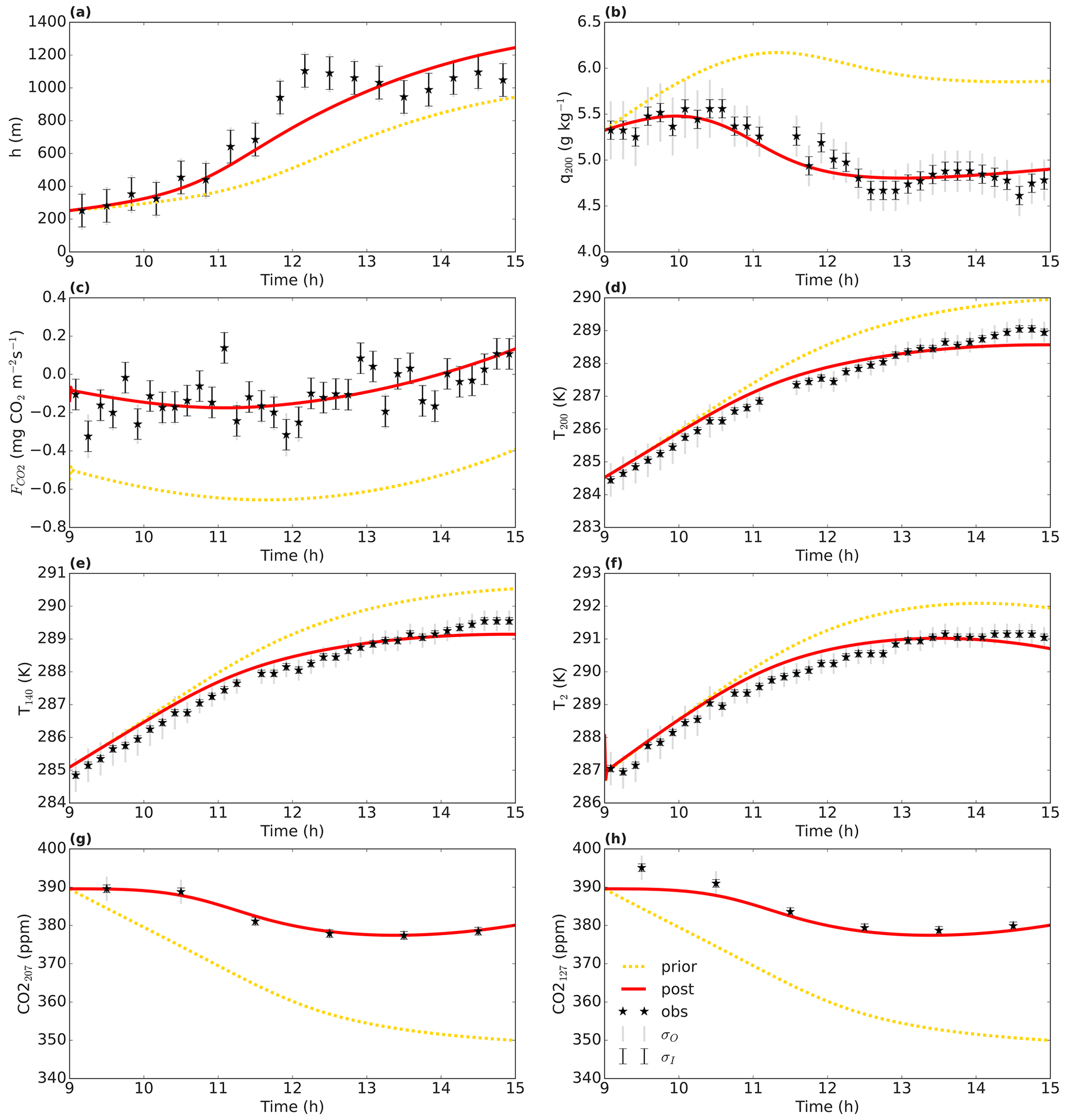
Figure 5Optimisation for the Cabauw data. The full red line shows the optimised model (“post” means posterior), and the dotted yellow line is the prior model. The observations are shown by a black star. The error bars show the measurement error standard deviation σI and total error standard deviation σO on the observations.
9.6 Posterior uncertainty and correlations
The discussion above illustrates that not all of the parameters in the state may be assumed to be fully independent. To analyse the posterior correlations, we have constructed a correlation matrix (Sect. 4.2), as shown in Fig. 7. From the 174 perturbed ensemble members, 150 were successful and were used for the calculation of statistics. As expected, the correlation between αsto and R10 is very strongly positive (0.94), and this can likely be explained by their opposite effects on the CO2 flux, as explained in the previous paragraph. Some of the correlations between parameters can be relatively complex, e.g. a correlation between two posterior parameters might involve a third parameter that correlates with both.
Coming back to the discrepancy in CO2 advection between our analysis and what was found by Casso-Torralba et al. (2008), it can be noted that the adv parameter is relatively strongly correlated with both the and parameters (Fig. 7; correlation of −0.65 and −0.80, respectively). This can indicate that entrainment from the free troposphere is hard to disentangle from advection in shaping the CO2 budget, with the current set of observations we incorporate. Differences in how entrainment is handled by Casso-Torralba et al. (2008) might explain part of the difference in estimated CO2 advection.
To check to what extent the obtained correlations are robust and independent of the selected number of ensemble members, we reconstructed the correlation matrix using only half of the successful perturbed members (75 of the 150). The average absolute value of difference between the non-diagonal matrix entries when using the subsample and the non-diagonal matrix entries when using the full successful perturbed ensemble amounts to 0.05, with a maximum of 0.23 for one entry. This suggests that using 150 members in the correlation analysis leads to a reasonably robust estimate of the posterior correlations.
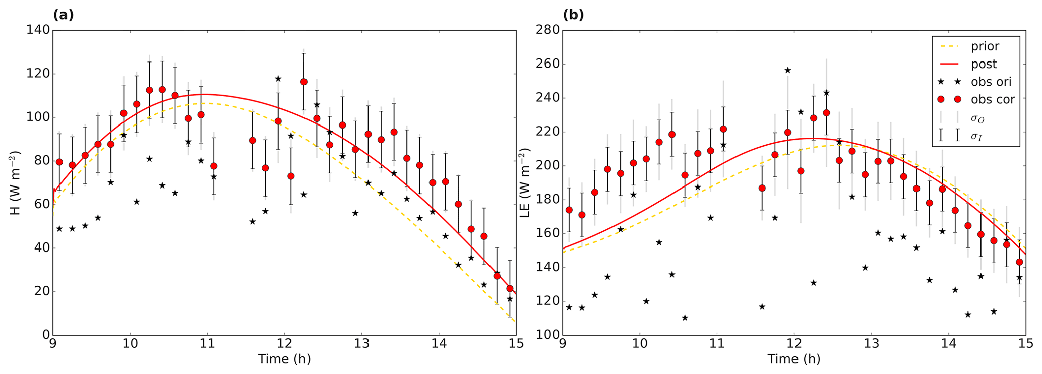
Figure 6Energy balance data, with (a) sensible heat flux and (b) latent heat flux, for the Cabauw case. The black stars are the original observations, and the red dots the observations after forced closure of the energy balance. The error bars indicate the measurement error standard deviation σI and the total observational error standard deviation σO. The full red line shows the optimised model (“post” means posterior), and the dashed yellow line is the prior model.
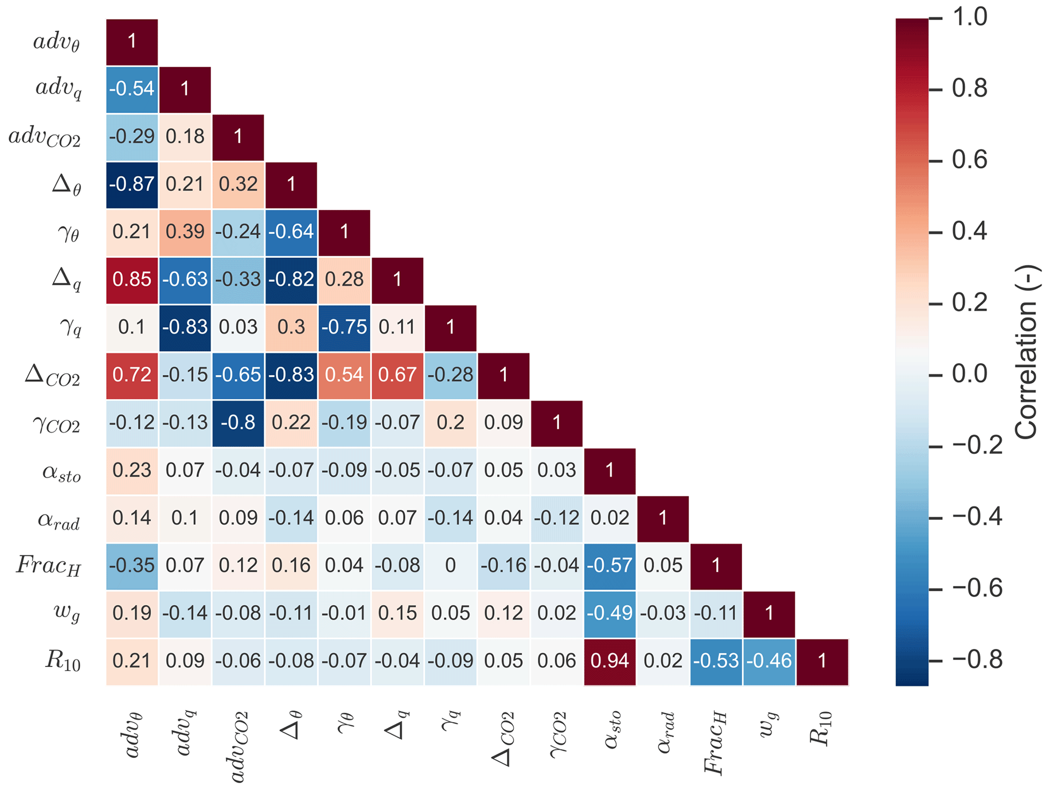
Figure 7Correlation matrix for the optimised state parameters for the Cabauw case. The shown correlations are marginal correlations and not partial correlations.
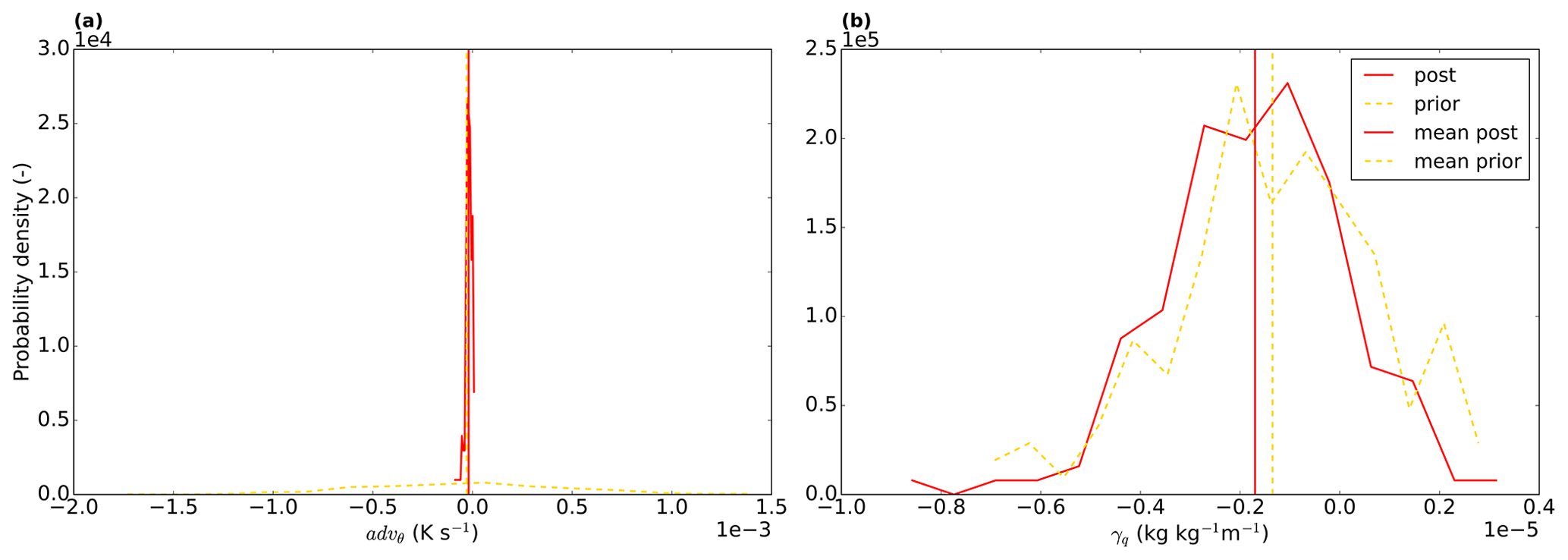
Figure 8Probability density functions for the advθ (a) and γq (b) parameters. The red full line is for the posterior and the yellow dashed line for the prior distribution. The vertical lines represent the mean of the distributions. For each probability density function, 15 bins were used. Note that the prior distribution is determined from the sample of priors, which has a component of randomness.
Another option we explore is to analyse the posterior pdf's for the successful perturbed members in the ensemble. As an example, we show the pdf's for two parameters, advθ and γq (Fig. 8). For advθ, the posterior uncertainty is clearly reduced compared to the prior, as the posterior pdf is markedly narrower. For γq (the free-tropospheric specific humidity lapse rate), however, there is no clear reduction in uncertainty. The wide posterior pdf implies that similar results can be obtained over a relatively wide range of γq, possibly by perturbing other parameters with a similar effect. To further constrain this parameter, more specific observation streams would need to be added, possibly from radiosondes. The use of ICLASS in, for example, the planning of observational campaigns can therefore help to determine beforehand what type of observations are needed to better constrain the processes represented in the model. This is done through the use of observation system simulation experiments, similar to, for example, Ye et al. (2022).
We have presented here a description of ICLASS, a variational Inverse modelling framework for the Chemistry Land-surface Atmosphere Soil Slab model. This framework serves as a tool to study the atmospheric boundary layer and/or land–atmosphere exchange. It avoids the need for manual trial-and-error in choosing parameter values for the model when fitting observations, thereby providing more objectivity. Some extent of subjectivity, however, remains, as the proper specification of errors is not always simple (e.g. Rödenbeck et al., 2003). The use of more advanced error estimation methods can mitigate this. The very non-linear model around which the framework is built makes the optimisation challenging. In ICLASS, two main ways in which this challenge is tackled are as follows:
-
The use of an analytical gradient of the cost function involving the model adjoint, thus allowing for more precise gradient calculations.
-
The possibility of running ICLASS in a Monte Carlo way. This involves perturbing the prior state vector and the (scaled) observations. When a single optimisation does not converge, then the use of an ensemble can provide a solution.
The latter way of running ICLASS also has the advantage that posterior error statistics can be obtained, which is of paramount importance in inverse modelling.
The model is relatively simple yet contains the physics to model the essentials of the convective boundary layer and of land surface–atmosphere exchange. Its simplicity, however, means that the model does not perform well in every situation. The best performance can be expected for days when the boundary layer resembles a prototypical convective boundary layer. We have shown the usefulness of ICLASS by applying it to a golden day at a Dutch grassland site where extensive data are available. The fit to several streams of observations simultaneously was greatly improved in the posterior compared to the prior. We have to keep in mind, however, that we cannot expect a relatively simple model to capture all small-scale processes playing a role in the convective boundary layer and in land surface–atmosphere exchange (e.g. heterogeneous surface heating, heterogeneous evaporation and influence of individual thermals).
Key strengths of this framework are that observations from several information streams can be used simultaneously, and surface layer profiles can be taken into account. The framework allows the integration of knowledge from ecosystem-level studies (fluxes) and global studies (mixing ratios). It can be seen as a tool that maximises the use of available observational data at CBL/ecosystem level (e.g. along tall towers like the Cabauw tower). Observation system simulation experiments using ICLASS can also help in the planning of observational campaigns so as to determine in advance which observation streams are needed to better constrain model processes. Another feature of the framework is the capacity of correcting observations for biases. A specific bias correction system for the energy balance closure problem is implemented. The energy balance residual was shown to be substantial at the Dutch grassland site in our application example. Correcting for biases is critical in inverse modelling to prevent bias errors from propagating in parameter estimates. The correction of biases is, however, a very complex topic. There are limitations to the level of complexity that our bias correction methods can handle, and ICLASS cannot be expected to deal completely with all bias issues.
ICLASS is computationally relatively cheap to run and can be extended in the future by, for example, incorporating a more detailed representation of the vegetation. This extension can further improve the capabilities to fit sets of observations at locations with a more complex vegetation structure.

Table A2Used observation streams in this paper. Note that variables such as T200 and T140 are called Tmh and Tmh2, respectively, in the model code for Sect. 9, which represents temperatures at the user-specified temperature measuring heights 1 and 2, respectively. For the CO2 mixing ratio, we do not make a distinction in this paper between the moist-air and dry-air mixing ratio.
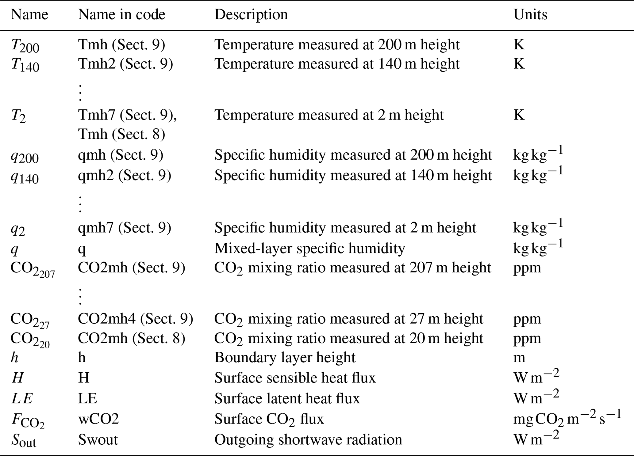

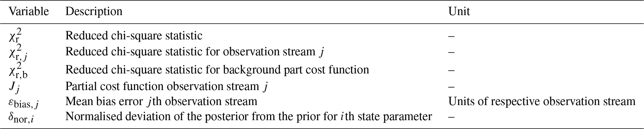
The code is hosted at GitHub. The current version of ICLASS is available from https://github.com/PBosmanatm/ICLASS (last access: 9 December 2022) under a GNU General Public License, v3.0 or later. The adapted forward model and the ICLASS manual are also included in the GitHub repository. This repository is linked to Zenodo, which provides DOIs for released software. The release on which this reference paper is based can be found at https://doi.org/10.5281/zenodo.7239147 (Bosman and Krol, 2022) (GNU General Public License, v3.0 or later). The code and the data used for creating the plots with optimisation results in this paper, and for the content of the tables, are part of the downloadable material. The data used in this paper can differ somewhat from the most recent version of these data. Boundary layer height data were provided by Henk Klein Baltink (KNMI). These data (and all other used data) can be found via the Zenodo link. The newest version of the Cabauw data (except for boundary layer heights) can be found at the following locations: the CO2 mixing ratios can be found at the ICOS (https://www.icos-cp.eu/data-products/ERE9-9D85, https://doi.org/10.18160/ERE9-9D85, Drought 2018 Team and ICOS Atmosphere Thematic Centre, 2020) and ObsPack (https://gml.noaa.gov/ccgg/obspack/, The Global Monitoring Laboratory of the National Oceanic and Atmospheric Administration, 2022) websites. Temperature, heat fluxes, and so on can be found at https://dataplatform.knmi.nl/dataset/?tags=Insitu&tags=CESAR (KNMI, 2022).
The supplement related to this article is available online at: https://doi.org/10.5194/gmd-16-47-2023-supplement.
MCK and PJMB designed the study. PJMB performed the majority of the coding and adjoint model construction, with help from MCK. PJMB performed the numerical optimisations and wrote the paper, the latter with help from MCK.
The contact author has declared that neither of the authors has any competing interests.
Publisher's note: Copernicus Publications remains neutral with regard to jurisdictional claims in published maps and institutional affiliations.
This work is part of the COS-OCS project (http://cos-ocs.eu/, last access: 9 December 2022), a project that received funding from the European Research Council (ERC) under the European Union's Horizon 2020 Research and Innovation programme (grant no. 742798). Part of this work was carried out on the Dutch national e-infrastructure, with the support of SURF Cooperative. We are grateful to Jordi Vilà-Guerau De Arellano, Fred Bosveld, Arnoud Frumau, and Henk Klein Baltink, for helping us with and/or providing (directly or indirectly) the Cabauw data. We would also like to thank the developers of the CLASS model. Thanks also to the three anonymous reviewers, for helping us to improve the paper. We furthermore thank Chiel van Heerwaarden, Linda Kooijmans, and Jordi Vilà-Guerau De Arellano for providing comments on an earlier version of this work.
This research has been supported by the European Research Council under the European Union's Horizon 2020 Research and Innovation programme (COS-OCS; grant no. 742798).
This paper was edited by Jinkyu Hong and reviewed by three anonymous referees.
Barbaro, E., Vilà-Guerau de Arellano, J., Ouwersloot, H. G., Schröter, J. S., Donovan, D. P., and Krol, M. C.: Aerosols in the convective boundary layer: Shortwave radiation effects on the coupled land-atmosphere system, J. Geophys. Res.-Atmos., 119, 5845–5863, https://doi.org/10.1002/2013JD021237, 2014. a
Bastrikov, V., MacBean, N., Bacour, C., Santaren, D., Kuppel, S., and Peylin, P.: Land surface model parameter optimisation using in situ flux data: comparison of gradient-based versus random search algorithms (a case study using ORCHIDEE v1.9.5.2), Geosci. Model Dev., 11, 4739–4754, https://doi.org/10.5194/gmd-11-4739-2018, 2018. a, b, c
Bergamaschi, P., Frankenberg, C., Meirink, J. F., Krol, M., Villani, M. G., Houweling, S., Dentener, F., Dlugokencky, E. J., Miller, J. B., Gatti, L. V., Engel, A., and Levin, I.: Inverse modeling of global and regional CH4 emissions using SCIAMACHY satellite retrievals, J. Geophys. Res.-Atmos., 114, 1–28, https://doi.org/10.1029/2009JD012287, 2009. a
Bosman, P. and Krol, M.: PBosmanatm/ICLASS: ICLASS v1.1, Zenodo [code and data set], https://doi.org/10.5281/zenodo.7239147, 2022. a
Bosveld, F., Van Meijgaard, E., Moors, E., and Werner, C.: Interpretation of flux observations along the Cabauw 200 m meteorological tower, in: 16th Symposium on Boundary Layers and Turbulence 6.18, 1–4, Portland, USA, https://ams.confex.com/ams/BLTAIRSE/webprogram/Paper78632.html (last access: 9 December 2022), 2004. a
Bosveld, F. C., Baas, P., Beljaars, A. C. M., Holtslag, A. A. M., de Arellano, J. V.-G., and van de Wiel, B. J. H.: Fifty Years of Atmospheric Boundary-Layer Research at Cabauw Serving Weather, Air Quality and Climate, Bound.-Lay. Meteorol., 177, 583–612, https://doi.org/10.1007/s10546-020-00541-w, 2020. a, b
Brasseur, G. and Jacob, D.: Inverse Modeling for Atmospheric Chemistry, in: Modeling of Atmospheric Chemistry, Cambridge University Press, Cambridge, 487–537, https://doi.org/10.1017/9781316544754.012, 2017. a, b, c, d, e, f
Casso-Torralba, P., de Arellano, J. V. G., Bosveld, F., Soler, M. R., Vermeulen, A., Werner, C., and Moors, E.: Diurnal and vertical variability of the sensible heat and carbon dioxide budgets in the atmospheric surface layer, J. Geophys. Res.-Atmos., 113, D12119, https://doi.org/10.1029/2007JD009583, 2008. a, b, c, d, e
Chevallier, F.: Impact of correlated observation errors on inverted CO2 surface fluxes from OCO measurements, Geophys. Res. Lett., 34, L24804, https://doi.org/10.1029/2007GL030463, 2007. a
Chevallier, F., Fisher, M., Peylin, P., Serrar, S., Bousquet, P., Bréon, F.-M., Chédin, A., and Ciais, P.: Inferring CO2 sources and sinks from satellite observations: Method and application to TOVS data, J. Geophys. Res., 110, D24309, https://doi.org/10.1029/2005JD006390, 2005. a
Chevallier, F., Bréon, F.-M., and Rayner, P. J.: Contribution of the Orbiting Carbon Observatory to the estimation of CO2 sources and sinks: Theoretical study in a variational data assimilation framework, J. Geophys. Res., 112, D09307, https://doi.org/10.1029/2006JD007375, 2007. a
Chevallier, F., Ciais, P., Conway, T. J., Aalto, T., Anderson, B. E., Bousquet, P., Brunke, E. G., Ciattaglia, L., Esaki, Y., Fröhlich, M., Gomez, A., Gomez-Pelaez, A. J., Haszpra, L., Krummel, P. B., Langenfelds, R. L., Leuenberger, M., Machida, T., Maignan, F., Matsueda, H., Morguí, J. A., Mukai, H., Nakazawa, T., Peylin, P., Ramonet, M., Rivier, L., Sawa, Y., Schmidt, M., Steele, L. P., Vay, S. A., Vermeulen, A. T., Wofsy, S., and Worthy, D.: CO2 surface fluxes at grid point scale estimated from a global 21 year reanalysis of atmospheric measurements, J. Geophys. Res., 115, D21307, https://doi.org/10.1029/2010JD013887, 2010. a
Claerbout, J. F.: Earth soundings analysis: processing versus inversion, Blackwell Scientific Publications, Cambridge, http://sep.stanford.edu/sep/prof/pvi.pdf (last access: 9 December 2022), 2004. a, b
Commane, R., Meredith, L. K., Baker, I. T., Berry, J. A., Munger, J. W., Montzka, S. A., Templer, P. H., Juice, S. M., Zahniser, M. S., and Wofsy, S. C.: Seasonal fluxes of carbonyl sulfide in a midlatitude forest, P. Natl. Acad. Sci. USA, 112, 14162–14167, 2015. a
Doicu, A., Trautmann, T., and Schreier, F.: Numerical Regularization for Atmospheric Inverse Problems, Springer Praxis Books in environmentral sciences, https://doi.org/10.1007/978-3-642-05439-6, 2010. a
Drought 2018 Team and ICOS Atmosphere Thematic Centre: Drought-2018 atmospheric CO2 Mole Fraction product for 48 stations (96 sample heights), https://doi.org/10.18160/ERE9-9D85, 2020. a
Elizondo, D., Faure, C., and Cappelaere, B.: Automatic- versus Manual- differentiation for non-linear inverse modeling, Tech. rep., INRIA (Institut National de Recherche en Informatique et en Automatique), https://hal.inria.fr/inria-00072666/document (last access: 9 December 2022), 2000. a, b
Foken, T.: The Energy Balance Closure Problem: An Overview, Ecol. Appl., 18, 1351–1367, 2008. a, b, c, d, e
Friend, A. D.: Modelling Canopy CO2 Fluxes: Are “Big-Leaf” Simplifications Justified?, Global Ecol. Biogeogr., 10, 603–619, 2001. a
Henze, D. K., Hakami, A., and Seinfeld, J. H.: Development of the adjoint of GEOS-Chem, Atmospheric Chemistry and Physics, 7, 2413–2433, https://doi.org/10.5194/acp-7-2413-2007, 2007. a
Honnorat, M., Marin, J., Monnier, J., and Lai, X.: Dassflow v1.0: a variational data assimilation software for 2D river flows, Tech. rep., INRIA (Institut National de Recherche en Informatique et en Automatique), http://hal.inria.fr/inria-00137447 (last access: 9 December 2022), 2007. a, b
Hunter, J.: Matplotlib: A 2D Graphics Environment, Comput. Sci. Eng., 9, 90–95, https://doi.org/10.1109/MCSE.2007.55, 2007. a
Jacobs, C.: Direct impact of atmospheric CO2 enrichment on regional transpiration, PhD thesis, Wageningen University, ISBN 9789054852506, 1994. a, b, c
Jarvis, P.: The interpretation of the variations in leaf water potential and stomatal conductance found in canopies in the field, Philos. T. Roy. Soc. Lond. B, 273, 593–610, https://doi.org/10.1098/rstb.1976.0035, 1976. a
Kaminski, T., Knorr, W., Scholze, M., Gobron, N., Pinty, B., Giering, R., and Mathieu, P.-P.: Consistent assimilation of MERIS FAPAR and atmospheric CO2 into a terrestrial vegetation model and interactive mission benefit analysis, Biogeosciences, 9, 3173–3184, https://doi.org/10.5194/bg-9-3173-2012, 2012. a
Krol, M. C., Meirink, J. F., Bergamaschi, P., Mak, J. E., Lowe, D., Jöckel, P., Houweling, S., and Röckmann, T.: What can 14CO measurements tell us about OH?, Atmospheric Chemistry and Physics, 8, 5033–5044, https://doi.org/10.5194/acp-8-5033-2008, 2008. a
Liu, H., Randerson, J. T., Lindfors, J., Massman, W. J., and Foken, T.: Consequences of incomplete surface energy balance closure for CO2 fluxes from open-path CO2/H2O infrared gas analysers, Bound.-Lay. Meteorol., 120, 65–85, https://doi.org/10.1007/s10546-005-9047-z, 2006. a
Ma, J., Kooijmans, L. M. J., Cho, A., Montzka, S. A., Glatthor, N., Worden, J. R., Kuai, L., Atlas, E. L., and Krol, M. C.: Inverse modelling of carbonyl sulfide: implementation, evaluation and implications for the global budget, Atmos. Chem. Phys., 21, 3507–3529, https://doi.org/10.5194/acp-21-3507-2021, 2021. a
Mäkelä, J., Knauer, J., Aurela, M., Black, A., Heimann, M., Kobayashi, H., Lohila, A., Mammarella, I., Margolis, H., Markkanen, T., Susiluoto, J., Thum, T., Viskari, T., Zaehle, S., and Aalto, T.: Parameter calibration and stomatal conductance formulation comparison for boreal forests with adaptive population importance sampler in the land surface model JSBACH, Geosci. Model Dev., 12, 4075–4098, https://doi.org/10.5194/gmd-12-4075-2019, 2019. a
Margulis, S. A. and Entekhabi, D.: A Coupled Land Surface–Boundary Layer Model and Its Adjoint, J. Hydrometeorol., 2, 274–296, https://doi.org/10.1175/1525-7541(2001)002<0274:ACLSBL>2.0.CO;2, 2001a. a
Margulis, S. A. and Entekhabi, D.: Feedback between the land surface energy balance and atmospheric boundary layer diagnosed through a model and its adjoint, J. Hydrometeorol., 2, 599–620, https://doi.org/10.1175/1525-7541(2001)002<0599:FBTLSE>2.0.CO;2, 2001b. a
McNorton, J., Wilson, C., Gloor, M., Parker, R. J., Boesch, H., Feng, W., Hossaini, R., and Chipperfield, M. P.: Attribution of recent increases in atmospheric methane through 3-D inverse modelling, Atmos. Chem. Phys., 18, 18149–18168, https://doi.org/10.5194/acp-18-18149-2018, 2018. a
Meirink, J. F., Bergamaschi, P., and Krol, M. C.: Four-dimensional variational data assimilation for inverse modelling of atmospheric methane emissions: method and comparison with synthesis inversion, Atmos. Chem. Phys., 8, 6341–6353, https://doi.org/10.5194/acp-8-6341-2008, 2008. a, b
Michalak, A. M., Hirsch, A., Bruhwiler, L., Gurney, K. R., Peters, W., and Tans, P. P.: Maximum likelihood estimation of covariance parameters for Bayesian atmospheric trace gas surface flux inversions, J. Geophys. Res.-Atmos., 110, D24107, https://doi.org/10.1029/2005JD005970, 2005. a, b
Miller, S. M., Michalak, A. M., and Levi, P. J.: Atmospheric inverse modeling with known physical bounds: an example from trace gas emissions, Geosci. Model Dev., 7, 303–315, https://doi.org/10.5194/gmd-7-303-2014, 2014. a
Monin, A. and Obukhov, A.: Basic laws of turbulent mixing in the atmosphere near the ground, Tr. Akad. Nauk SSSR Geophiz. Inst., 24, 1963–1987, 1954. a
Nash, S. G.: A survey of truncated-Newton methods, J. Comput. Appl. Math., 124, 45–59, https://doi.org/10.1016/S0377-0427(00)00426-X, 2000. a, b
Oncley, S. P., Foken, T., Vogt, R., Kohsiek, W., DeBruin, H. A. R., Bernhofer, C., Christen, A., van Gorsel, E., Grantz, D., Feigenwinter, C., Lehner, I., Liebethal, C., Liu, H., Mauder, M., Pitacco, A., Ribeiro, L., and Weidinger, T.: The Energy Balance Experiment EBEX-2000. Part I: overview and energy balance, Bound.-Lay. Meteorol., 123, 1–28, https://doi.org/10.1007/s10546-007-9161-1, 2007. a, b
Ouwersloot, H. G., Vilà-Guerau de Arellano, J., Nölscher, A. C., Krol, M. C., Ganzeveld, L. N., Breitenberger, C., Mammarella, I., Williams, J., and Lelieveld, J.: Characterization of a boreal convective boundary layer and its impact on atmospheric chemistry during HUMPPA-COPEC-2010, Atmos. Chem. Phys., 12, 9335–9353, https://doi.org/10.5194/acp-12-9335-2012, 2012. a
Raoult, N. M., Jupp, T. E., Cox, P. M., and Luke, C. M.: Land-surface parameter optimisation using data assimilation techniques: the adJULES system V1.0, Geosci. Model Dev., 9, 2833–2852, https://doi.org/10.5194/gmd-9-2833-2016, 2016. a, b, c
Renner, M., Brenner, C., Mallick, K., Wizemann, H.-D., Conte, L., Trebs, I., Wei, J., Wulfmeyer, V., Schulz, K., and Kleidon, A.: Using phase lags to evaluate model biases in simulating the diurnal cycle of evapotranspiration: a case study in Luxembourg, Hydrol. Earth Syst. Sci., 23, 515–535, https://doi.org/10.5194/hess-23-515-2019, 2019. a, b, c
Rödenbeck, C., Houweling, S., Gloor, M., and Heimann, M.: CO2 flux history 1982–2001 inferred from atmospheric data using a global inversion of atmospheric transport, Atmos. Chem. Phys., 3, 1919–1964, https://doi.org/10.5194/acp-3-1919-2003, 2003. a
Ronda, R. J., de Bruin, H. A. R., and Holtslag, A.: Representation of the Canopy Conductance in Modeling the Surface Energy Budget for Low Vegetation, Am. Meteorol. Soc., 40, 1431–1444, 2001. a, b
Santaren, D., Peylin, P., Bacour, C., Ciais, P., and Longdoz, B.: Ecosystem model optimization using in situ flux observations: benefit of Monte Carlo versus variational schemes and analyses of the year-to-year model performances, Biogeosciences, 11, 7137–7158, https://doi.org/10.5194/bg-11-7137-2014, 2014. a
Schulte, R., van Zanten, M., Rutledge-Jonker, S., Swart, D., Wichink Kruit, R., Krol, M., van Pul, W., and Vilà-Guerau de Arellano, J.: Unraveling the diurnal atmospheric ammonia budget of a prototypical convective boundary layer, Atmo. Environ., 249, 118153, https://doi.org/10.1016/J.ATMOSENV.2020.118153, 2021. a
Schürmann, G. J., Kaminski, T., Köstler, C., Carvalhais, N., Voßbeck, M., Kattge, J., Giering, R., Rödenbeck, C., Heimann, M., and Zaehle, S.: Constraining a land-surface model with multiple observations by application of the MPI-Carbon Cycle Data Assimilation System V1.0, Geosci. Model Dev., 9, 2999–3026, https://doi.org/10.5194/gmd-9-2999-2016, 2016. a
Stewart, J.: Modelling surface conductance of pine forest, Agr. Forest Meteoro., 43, 19–35, https://doi.org/10.1016/0168-1923(88)90003-2, 1988. a
Stull, R. B.: An introduction to boundary layer meteorology, Kluwer Academic Publishers, Dordrecht, https://doi.org/10.1007/978-94-009-3027-8, 1988. a, b, c
Tang, J. and Zhuang, Q.: Equifinality in parameterization of process-based biogeochemistry models: A significant uncertainty source to the estimation of regional carbon dynamics, J. Geophys. Res.-Biogeo., 113, https://doi.org/10.1029/2008JG000757, 2008. a
Tarantola, A.: Inverse problem theory and methods for model parameter estimation, in: Other Titles in Applied Mathematics, Society for Industrial and Applied Mathematics (siam), Philadelphia, USA, https://doi.org/10.1137/1.9780898717921, 2005. a, b
The Global Monitoring Laboratory of the National Oceanic and Atmospheric Administration: Observation Package (ObsPack) Data Products, https://gml.noaa.gov/ccgg/obspack/, last access: 9 December 2022. a
The Royal Netherlands Meteorological Institute (KNMI): KNMI Data Platform, https://dataplatform.knmi.nl/dataset/?tags=Insitu&tags=CESAR, last access: 9 December 2022. a
The SciPy community: scipy.optimize.fmin_tnc, https://docs.scipy.org/doc/scipy/reference/generated/scipy.optimize.fmin_tnc.html, last access: 9 December 2022. a
van der Walt, S., Colbert, S., and Varoquaux, G.: The NumPy Array: A Structure for Efficient Numerical Computation, Comput. Sci. Eng., 13, 22–30, https://doi.org/10.1109/MCSE.2011.37, 2011. a
van Heerwaarden, C. C., Vilà-Guerau de Arellano, J., Moene, A. F., and Holtslag, A. A. M.: Interactions between dry-air entrainment, surface evaporation and convective boundary-layer development, Q. J. Roy. Meteor. Soc., 135, 1277–1291, https://doi.org/10.1002/qj.431, 2009. a
van Heerwaarden, C. C., Vilà-Guerau de Arellano, J., Gounou, A., Guichard, F., and Couvreux, F.: Understanding the daily cycle of evapotranspiration: A method to quantify the influence of forcings and feedbacks, J. Hydrometeorol., 11, 1405–1422, https://doi.org/10.1175/2010JHM1272.1, 2010. a
Vermeulen, A. T., Hensen, A., Popa, M. E., van den Bulk, W. C. M., and Jongejan, P. A. C.: Greenhouse gas observations from Cabauw Tall Tower (1992–2010), Atmos. Meas. Tech., 4, 617–644, https://doi.org/10.5194/amt-4-617-2011, 2011. a
Vesala, T., Suni, T., Rannik, Ü., Keronen, P., Markkanen, T., Sevanto, S., Grönholm, T., Smolander, S., Kulmala, M., Ilvesniemi, H., Ojansuu, R., Uotila, A., Levula, J., Mäkelä, A., Pumpanen, J., Kolari, P., Kulmala, L., Altimir, N., Berninger, F., Nikinmaa, E., and Hari, P.: Effect of thinning on surface fluxes in a boreal forest, Global Biogeochem. Cy., 19, GB2001, https://doi.org/10.1029/2004GB002316, 2005. a
Vilà-Guerau De Arellano, J., Van Heerwaarden, C. C., and Lelieveld, J.: Modelled suppression of boundary-layer clouds by plants in a CO2-rich atmosphere, Nat. Geosci., 5, 701–704, https://doi.org/10.1038/ngeo1554, 2012. a, b, c, d
Vilà-Guerau De Arellano, J., Van Heerwaarden, C. C., Van Stratum, B. J., and Van Den Dries, K.: Atmospheric boundary layer: Integrating air chemistry and land interactions, Cambridge University Press, https://doi.org/10.1017/CBO9781316117422, 2015. a, b, c
Whelan, M. E., Lennartz, S. T., Gimeno, T. E., Wehr, R., Wohlfahrt, G., Wang, Y., Kooijmans, L. M. J., Hilton, T. W., Belviso, S., Peylin, P., Commane, R., Sun, W., Chen, H., Kuai, L., Mammarella, I., Maseyk, K., Berkelhammer, M., Li, K.-F., Yakir, D., Zumkehr, A., Katayama, Y., Ogée, J., Spielmann, F. M., Kitz, F., Rastogi, B., Kesselmeier, J., Marshall, J., Erkkilä, K.-M., Wingate, L., Meredith, L. K., He, W., Bunk, R., Launois, T., Vesala, T., Schmidt, J. A., Fichot, C. G., Seibt, U., Saleska, S., Saltzman, E. S., Montzka, S. A., Berry, J. A., and Campbell, J. E.: Reviews and syntheses: Carbonyl sulfide as a multi-scale tracer for carbon and water cycles, Biogeosciences, 15, 3625–3657, https://doi.org/10.5194/bg-15-3625-2018, 2018. a, b
Wouters, H., Petrova, I. Y., van Heerwaarden, C. C., Vilà-Guerau de Arellano, J., Teuling, A. J., Meulenberg, V., Santanello, J. A., and Miralles, D. G.: Atmospheric boundary layer dynamics from balloon soundings worldwide: CLASS4GL v1.0, Geosci. Model Dev., 12, 2139–2153, https://doi.org/10.5194/gmd-12-2139-2019, 2019. a
Ye, H., You, W., Zang, Z., Pan, X., Wang, D., Zhou, N., Hu, Y., Liang, Y., and Yan, P.: Observing system simulation experiment (OSSE)-quantitative evaluation of lidar observation networks to improve 3D aerosol forecasting in China, Atmo. Res., 270, 106069, https://doi.org/10.1016/j.atmosres.2022.106069, 2022. a
Ziehn, T., Scholze, M., and Knorr, W.: On the capability of Monte Carlo and adjoint inversion techniques to derive posterior parameter uncertainties in terrestrial ecosystem models, Global Biogeochem. Cy., 26, GB3025, https://doi.org/10.1029/2011GB004185, 2012. a, b
- Abstract
- Introduction
- Forward model
- Inverse modelling framework
- Error statistics
- Output
- Technical details of the code
- Adjoint model validation
- Inverse modelling validation: observation system simulation experiments
- Application example: CO2 and boundary layer meteorology at a Dutch grassland
- Concluding discussion
- Appendix A: Description of used parameters and observation streams
- Appendix B: Inverse-modelling variables
- Code and data availability
- Author contributions
- Competing interests
- Disclaimer
- Acknowledgements
- Financial support
- Review statement
- References
- Supplement