IceTFT v1.0.0: interpretable long-term prediction of Arctic sea ice extent with deep learning

Due to global warming, the Arctic sea ice extent (SIE) is rapidly decreasing each year. According to the Intergovernmental Panel on Climate Change (IPCC) climate model projections, the summer Arctic will be nearly sea-ice-free in the 2050s of the 21st century, which will have a great impact on global climate change. As a result, accurate predictions of Arctic sea ice are of significant interest. In most current studies, the majority of deep-learning-based SIE prediction models focus on one-step prediction, and they not only have short lead times but also limited prediction skill. Moreover, these models often lack interpretability. In this study, we construct the Ice temporal fusion transformer (IceTFT) model, which mainly consists of the variable selection network (VSN), the long short-term memory (LSTM) encoder, and a multi-headed attention mechanism. We select 11 predictors for the IceTFT model, including SIE, atmospheric variables, and oceanic variables, according to the physical mechanisms affecting sea ice development. The IceTFT model can provide 12-month SIE directly, according to the inputs of the last 12 months. We evaluate the IceTFT model from the hindcasting experiments for 2019–2021 and prediction for 2022. For the hindcasting of 2019–2021, the average monthly prediction errors are less than 0.21 ×10⁶ km², and the September prediction errors are less than 0.1 ×10⁶ km², which is superior to the models from Sea Ice Outlook (SIO). For the prediction of September 2022, we submitted the prediction to the SIO in June 2022, and IceTFT still has higher prediction skill. Furthermore, the VSN in IceTFT can automatically adjust the weights of predictors and filter spuriously correlated variables. Based on this, we analyze the sensitivity of the selected predictors for the prediction of SIE. This confirms that the IceTFT model has a physical interpretability.

1 Introduction

Arctic sea ice is one of the vital components of the global climate system. Due to global warming, the temperature rise in the Arctic has accelerated. This phenomenon, known as Arctic amplification, has accelerated the melting of Arctic sea ice, which may have a potential impact on weather patterns and the climate of the Northern Hemisphere (Liu et al., 2013; Cohen et al., 2014). According to the Intergovernmental Panel on Climate Change (IPCC) climate model projections, the summer Arctic will be nearly sea-ice-free in the 2050s of the 21st century (Stroeve et al., 2012; Overland and Wang, 2013; Voosen, 2020), which will have a significant impact on global climate change. Therefore, it is important to predict the development of Arctic sea ice, which can be an important reference for studying and predicting global climate change trends. Over the past few decades, the Arctic Ocean has been warming (Polyakova et al., 2006), and Arctic sea ice is melting rapidly. The September Arctic sea ice extent (SIE) declined on average by about 14 % per decade from 1979 to 2013 and by about 50 % by 2020 (Johannessen et al., 2020; Ramsayer, 2020). The SIE in September 2020 is the second-lowest value from the National Snow and Ice Data Center (NSIDC) Sea Ice Index, V3 (SII; Fetterer et al., 2017), data (1979–2020). Rapid melting has made accurate SIE prediction difficult.

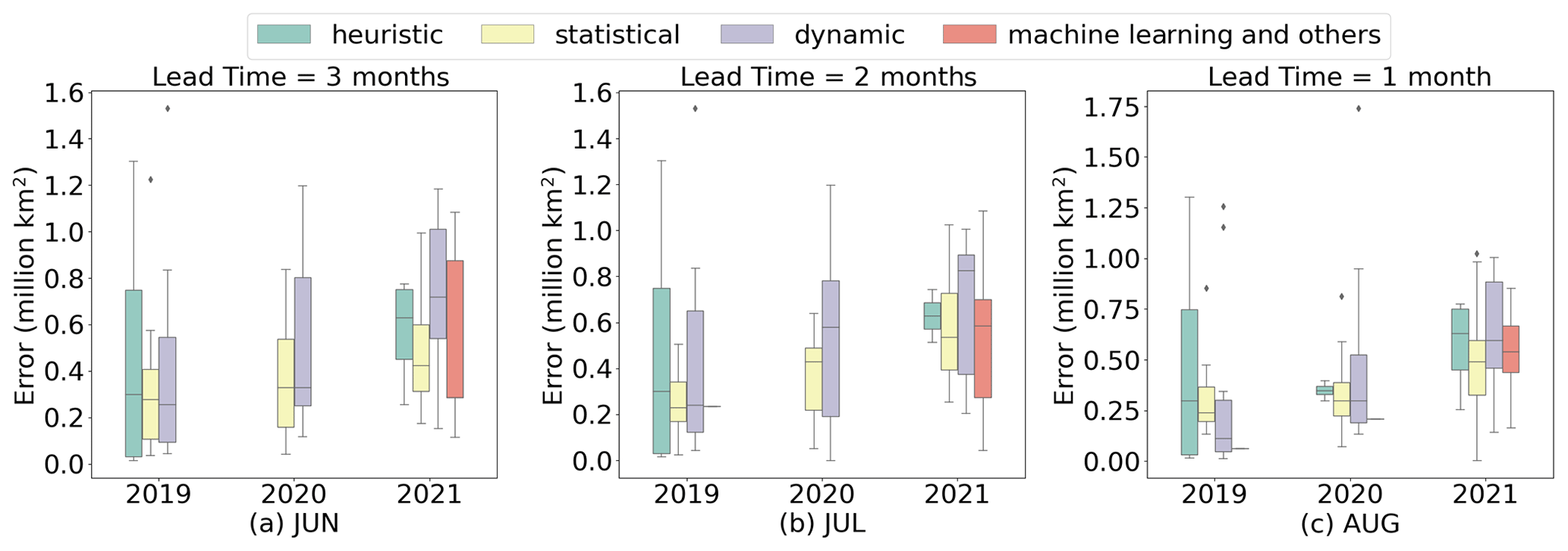
Figure 1 The September SIE prediction errors with a lead time of 3 (2,1) months from June (a) (July b; August c) for 2019–2021, which are published in the Sea Ice Outlook (SIO) by the Sea Ice Prediction Network (SIPN).

SIE is extremely cyclical and always reaches the maximum in March and the minimum in September (Kwok and Untersteiner, 2011). It is very difficult to predict the September minimum due to the influence of multiple physical factors. Figure 1a, b, and c show that the September SIE prediction errors with a lead time of 3 (2,1) months for 2019 to 2021, which are published in the Sea Ice Outlook (SIO) by Sea Ice Prediction Network (SIPN). Since 2008, the SIPN has collected September predictions annually, with a lead time of 1–3 months from global research institutions. And it represents the current prediction level and community knowledge of the state and evolution of Arctic sea ice on sub-seasonal to seasonal (S2S) timescales (Wei et al., 2021). From Fig. 1, it can be seen that there is still a clear gap between these predictions and observations. Surprisingly, the prediction skill did not improve significantly as the prediction lead time was reduced, which is consistent with another study (Stroeve et al., 2014). According to the SIO, we found more submissions for statistical approaches and dynamical models, while there were fewer submissions for machine learning until 2021. The medians of statistical approaches and machine learning are relatively close, and they both have slightly higher skills than dynamical models. However, due to the complexity of sea ice melt mechanisms, statistical models cannot capture the non-linear relationships between variables. As a result, deep learning can learn the features of the non-linear development of sea ice, which is extremely promising for sea ice prediction.

In recent years, deep learning methods have been increasingly used to predict sea ice levels. Chi and Kim (2017) first applied long short-term memory (LSTM) to a 1-month forecast model for the sea ice concentration (SIC) prediction. Then, they used a recursive approach to make the prediction model provide 12-month predictions. Kim et al. (2020) proposed a novel 1-month SIC prediction model, using convolutional neural networks (CNNs) that incorporate SIC, atmospheric variables, and oceanic variables. Due to the CNNs being unable to capture the time series dependence, they trained 12 models to produce predictions for each month and confirmed the superiority of these models. Andersson et al. (2021) proposed the IceNet model that learns from climate simulations and sea ice observation data. They also trained multiple models to provide months of predictions. Ren et al. (2022) proposed a purely data-driven model for daily SIC prediction called SICNet. They used an iteration method to obtain a weekly SIC prediction. In these studies, they focus on one-step models. To produce long-term predictions, they used a recursive approach, which can result in increasing errors, or they trained more models, which may increase the cost and time of computation. These studies highlight that long-term prediction has been less researched than short-term prediction. This ignores the periodicity of SIE. In addition, little attention has been paid to the explainability of the deep learning model. Chi et al. (2021) used ConvLSTM with a new perceptual loss function to predict SIC. Different variables were used as inputs of the proposed model for different channels, which does not provide insight into how the model utilizes the full channels of the input. These channel data may have an incomprehensible effect. Although the model in Andersson et al. (2021) was pre-trained with climate simulations, the effect on prediction is also unexplained. Compared to dynamic models, deep learning models are considered to be a “black box” due to the lack of physical mechanisms.

Our research team constructs deep learning models with interpretable and high prediction skill, based on the physical mechanisms of various weather and climate phenomena, which include the El Niño–Southern Oscillation (ENSO) and North Atlantic Oscillation (NAO; Mu et al., 2019, 2020, 2021, 2022). In this paper, to improve the long-term prediction skill for SIE and analyze the effects of various factors on SIE, we introduce a new SIE prediction model, based on the temporal fusion transformer (TFT; Lim et al., 2021), IceTFT, which is an interpretable model with high prediction skill. The IceTFT model can directly predict 12-month SIE through multi-horizon prediction. We select 11 predictors, based on the physical mechanisms and correlation analysis of Arctic sea ice, which include SIE, atmospheres, and ocean variables. The variable selection network (VSN) design in the IceTFT model species adjusts the weights of the variables by calculating their contribution to the prediction. On this basis, we can conduct sensitivity analysis experiments to quantify the role of predictors on the SIE prediction. The physical mechanisms affecting sea ice development can also be identified, which can provide a reference for selecting assimilation variables for dynamical models. In addition, we submitted the September prediction of 2022 to SIO in June 2022. The prediction skill of IceTFT, with a lead time of 9 months, outperforms most other models.

The contributions of this paper are as follows:

1. The IceTFT model uses LSTM encoders to summarize past inputs and generate context vectors, so it can directly provide a long-term prediction of SIE for up to 12 months. And it can predict September SIE 9 months in advance, which is longer than other studies with lead times of 1–3 months. IceTFT has the lowest prediction errors for hindcast experiments from 2019 to 2021 and the actual prediction of 2022, which was compared with SIO.

2. The IceTFT model is interpretable. It can automatically filter out spuriously correlated variables and adjust the weight of inputs through VSN, thus reducing noise interference in the input data. At the same time, it can also explore the contribution of different input variables to SIE predictions and reveal the physical mechanisms of sea ice development.

The remainder of the paper proceeds as follows: Sect. 2 introduces the proposed structure model called IceTFT. Section 3 deals with the atmospheric and oceanographic variables we selected. Section 4 introduces the evaluation metrics used. Section 5 presents the optimal setting of IceTFT model. The results of hindcasting experiments from 2019 to 2021 and of prediction for 2022 are presented in Sects. 6 and 7. Section 8 discusses the contribution of the inputs to the SIE predictions and gives an analysis of the physical mechanisms through which they affect sea ice.

2 IceTFT model

Deep learning has good performance in time series prediction, but previous research mostly used CNN and ConvLSTM, which still have high prediction errors. The transformer model makes the attention mechanism fully capture the temporal dependence, and it performs better than the traditional recurrent neural network (RNN) models (Vaswani et al., 2017). Based on the transformer model, a temporal fusion transformer (TFT) was proposed for multi-step prediction (Lim et al., 2021). TFT not only uses a sequence-to-sequence layer to learn both short-term and long-term temporal relationships at the local level but also uses a multi-head attention block to capture long-term dependencies. The VSN design in the TFT model species adjusts the weights of the variables and makes it interpretable. It has been verified that the TFT has small prediction errors in several areas.

The sea ice dataset is a time series with pronounced periodicity, which has a peak and a trough in a yearly cycle. These two peaks are usually critical to the prediction. And sea ice is affected by multiple physical factors, making its prediction more difficult. We propose the IceTFT model for SIE prediction, based on TFT, as follows:

1. The original design of TFT used known future data to support in the prediction of the primary time series data, since sea ice melting can be affected by various physical factors, and the various mechanisms responsible for sea ice variability have not yet been elucidated. To help the model learn the physical mechanisms underlying SIE, we modified that part to use atmospheric and oceanographic variables with the all the data at the same time as SIE.

2. The TFT relies on positional encoding to capture temporal features. When time series data are rolled into the model, the temporal information of the input data may be lost. To solve this problem, we set time-static metadata to provide temporal features that help the model better capture the periodicity of sea ice during the training process.

3. The original TFT uses quantile prediction as a loss function. Since SIE has decreased in recent years, there is some mutagenicity in summer. Therefore, the original design is not appropriate for predicting SIE. We used the mean square error (MSE) as the loss function to replace it.

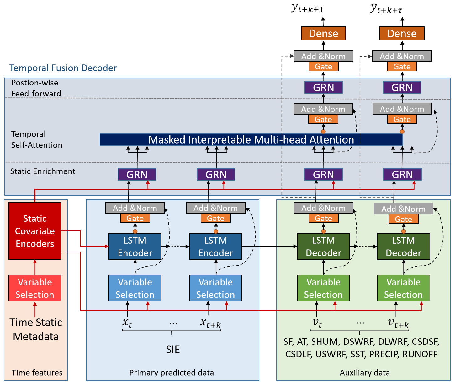
Figure 2 The IceTFT architecture is adapted on the basis of the original TFT (Lim et al., 2021). The time-static metadata, historical SIE data, and other atmospheric and oceanographic variables are all inputs to the IceTFT. The auxiliary data include snowfall (SF), 2 m air temperature (AT), 2 m surface air specific humidity (SHUM), downward shortwave radiative flux (DSWRF), downward longwave radiation flux (DLWRF), clear-sky downward longwave flux (CSDLF), clear-sky downward solar flux (CSDSF), upward solar radiation flux (USWRF), sea surface temperature (SST), precipitation (PRECIP), and river runoff (RUNOFF).

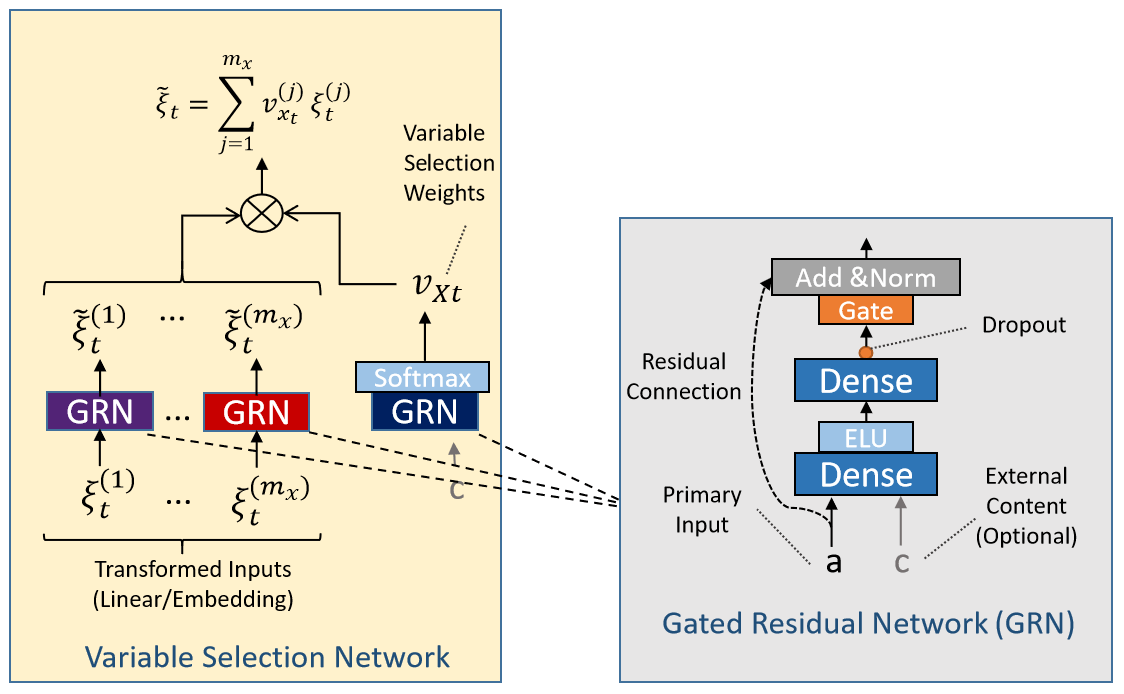
Figure 3 The components in IceTFT. The variable selection network (VSN) is used to select the most useful features. The gated residual network (GRN) enables efficient information flow by skipping connections and gating layers.

The IceTFT architecture is shown in Fig. 2. Three types of datasets are the inputs to IceTFT, which include time-static metadata, SIE, and other physical variables. And each type is selected by a VSN to filter out unnecessary noise. The structures of VSN and the gated residual network (GRN) are shown in Fig. 3. By using the GRN, the VSN calculates the weight of each variable contributing to the prediction, allowing the model to focus on the most significant features rather than overfitting irrelevant features. The VSN can also filter out spurious correlated variables to improve the accuracy of SIE predictions. This facilitates the analysis of the physical mechanisms underlying sea ice development and makes the IceTFT structure model more interpretable.

We can define the SIE prediction with IceTFT as a multi-variate spatiotemporal sequence prediction problem, as illustrated in Eq. (1).

$$\begin{array}{}\text{(1)}& {\displaystyle }\widehat{\mathrm{SIE}}=F_{\mathit{\theta }}\left(X\right),\left\{{\text{TIME}}_{\mathrm{static}},\mathrm{SIE},{\mathrm{VAR}}_{\mathrm{physical}}\right\}\subseteq X,\end{array}$$

where F_θ represents the IceTFT model (θ denotes the trainable parameters in the system). We have experimentally determined the optimal hyperparameters, and the size of the hidden layers is 160, the batch size is 128, the number of multi-head self-attentive mechanisms is 4, the dropout rate is 0.1, the max gradient norm is 0.01, and the learning rate is 0.001. $\widehat{\mathrm{SIE}}\in {\mathbb{R}}^{\mathrm{1}\times N}$ is the prediction result for future N months (N=12), and $X\in {\mathbb{R}}^{\mathrm{1}\times N}$ represents tree-type inputs in the historical N months (N=12). And the code source is available at Zenodo (https://doi.org/10.5281/zenodo.7409157, Luo, 2022). From Fig. 2, the first type of input, TIME_static, is time-static metadata calculated by counting days from the beginning of time. The IceTFT model is designed to use a static covariate encoder to integrate static features and to use GRN to generate different context vectors that are linked to the different locations. In the IceTFT model, we apply this design to provide temporal information so that the static covariate encoder conditions the temporal dynamics through these context vectors and so that the static enhancement layer enhances these temporal features. The second input is SIE, which is the primary data for prediction in the IceTFT structure model. The other inputs, VAR_physical, are various physical variables used to provide atmospheric and oceanographic features. IceTFT uses an LSTM encoder–decoder to enhance the locality information of these time series. This has the advantage of capturing anomalies and cycling with them. In addition, IceTFT uses an interpretable multi-head self-attentive mechanism to learn long-term features at different time steps. Each head can learn different temporal features and attend to a common set of inputs. Finally, to skip additional features, the outputs are processed by GRN in a position-wise feed-forward layer.

3 Predictors and datasets

As the subject of this research is the prediction of SIE, the historical data can provide data features for the SIE prediction. SIE is defined as the total area covered by grid cells with SIC > 15 %, which is a common metric used in sea ice analysis (Parkinson et al., 1999). The first dataset in the model is the monthly SIE, provided by the NSIDC Sea Ice Index, Version 3 (Fetterer et al., 2017). It contains daily and monthly SIE data in ASCII text files from November 1978 to the present. The area of this dataset is a region of the Arctic Ocean (39.23^∘ N–90^∘ N, 180^∘ W–180^∘ E), and the monthly SIE is derived from the daily SIE for each month.

Since the development of Arctic sea ice is influenced by a variety of physical factors such as the atmosphere and the ocean, we select a number of variables to support the proposed model for SIE prediction to help it learn more physical mechanisms and improve its prediction skill. Numerous studies have analyzed the causal relationship between sea ice and physical variables, due to the fact that fluctuations in sea ice can be generated by various dynamical and thermodynamic processes and other factors. Y. Huang et al. (2021) summarizes recent studies and known atmospheric processes associated with sea ice and presents the causality graph, as seen in Fig. 4.

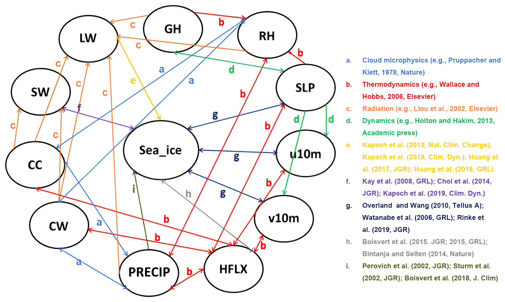
Figure 4 The causality graph derived from the study (Y. Huang et al., 2021) between important atmospheric variables and sea ice over the Arctic. Note that processes a–d (Pruppacher and Klett, 1978; Wallace and Hobbs, 2006; Liou, 2002; Holton and Hakim, 2013) are well-known atmospheric processes that can be outlined in several textbooks. Processes e–i (Kapsch et al., 2019; Huang et al., 2017, 2019; Kay and Wood, 2008; Choi et al., 2014; Overland and Wang, 2010; Watanabe et al., 2006; Rinke et al., 2019; Boisvert et al., 2015, 2018)) are summaries from recent peer-reviewed publications, and they are the subject of ongoing research. Sea ice here represents sea ice cover and/or sea ice thickness, GH is the geopotential height, RH is the relative humidity, SLP represents the sea level pressure, u10m and v10m represent meridional and zonal wind at 10 m, HFLX is the sensible plus latent heat flux, PRECIP is the total precipitation, CW is the total cloud water path, CC is the total cloud cover, and SW and LW represent the net shortwave and longwave flux at the surface, respectively.

From the study of Y. Huang et al. (2021), the arrows b and c in Fig. 4 show that the increase in the cloudiness and water vapor in the Arctic basin is due to local evaporation or enhanced water vapor transport, resulting in an increase in the downward longwave radiation flux (DLWRF; Luo et al., 2017). The DLWRF dominates surface warming and enhances sea ice melting in winter and spring (Kapsch et al., 2016, 2013). The melting of sea ice increases the air temperature, which in turn increases the DLWRF at the surface (Kapsch et al., 2013). At the same time, solar radiation may be absorbed by the ocean once the surface albedo is significantly reduced by sea ice melting, further accelerating sea ice melt in late spring and summer (Choi et al., 2014; Kapsch et al., 2016). Kapsch et al. (2016) studied the effects of realistic anomalies in the DLWRF and downward shortwave radiative flux (DSWRF) on sea ice by applying simplified forcing in a coupled climate model (arrows e and f in Fig. 4). In addition, Liu and Liu (2012) conducted numerical experiments with the MIT General Circulation Model (MITgcm), using a reanalysis dataset to demonstrate that changes in surface air temperature and DLWRF have played a significant role in the decline in the Arctic sea ice in recent years and that changes in surface air specific humidity (SHUM) can regulate the interannual variability in sea ice area. For our proposed model to learn the atmospheric process, we select the following variables: 2 m air temperature (AT), DSWRF, and DLWRF and the SHUM.

In addition, the snow layer can regulate the growth rate of sea ice because of its highly insulating properties, and the accumulation of precipitation on the sea ice pack significantly affects the depth of the snow layer (Sturm et al., 2002). Rain can melt, compact, and densify the snow layer, reducing the surface albedo and promoting sea ice melting (Perovich et al., 2002). The loss of snow on the ice leads to a significant reduction in the surface albedo over the Arctic Ocean, resulting in additional surface ice melt at the surface as more solar radiation is absorbed (Screen and Simmonds, 2012). Higher precipitation and snowfall can lead to a thicker snowpack, which affects sea ice change (Bintanja and Selten, 2014). Some researchers have studied the correlation between river runoff and sea ice and found that river runoff has some influence on sea ice melting (He-Ping et al., 2000; Tong et al., 2014). Precipitation at high latitudes would also increase Arctic river discharge, and river flow could have the positive effect of maintaining thicker ice (Weatherly and Walsh, 1996; arrow i in Fig. 4). Therefore, we also select precipitation (PRECIP), snowfall (SF), and river runoff (RUNOFF) so that the proposed model can learn these processes.

To improve the interpretability of the model, we also make it learn some ocean features in addition to atmospheric processes. Previous studies demonstrated the effects of sea surface temperature (SST) on Arctic sea ice. Bushuk and Giannakis (2017) found that SST provides an essential source of memory for the resurfacing of melt to growth re-emergence. Liang et al. (2019) supported that additional assimilation of SST improves the predictive accuracy of SIE and SIT in the marginal zone of sea ice. Therefore, we also selected SST variables to provide oceanographic features for the model.

The mean values of each of the above eight variables in the global region were used as input data for the model, and we calculated the correlation coefficient between them and SIE. The results are shown in Table 1. The variables with the highest correlation coefficient with SIE, as shown in Table 1, are SST, AT, RUNOFF, and DLWRF, which are shown in bold. And these variables are all connected to surface evaporation and surface heat in the Arctic hydrological cycle. To make the model learn more physical mechanisms, we selected clear-sky downward longwave flux (CSDLF), clear-sky downward solar flux (CSDSF), and upward solar radiation flux (USWRF) these radiative variables. A total of 11 physical variables are listed in Table 1.

Table 1 The names, types, sources, units of the 11 physical variables and their correlation coefficients with the SIE. The variables with the highest correlation coefficient with SIE are SST, AT, RUNOFF, and DLWRF, which are shown in bold.

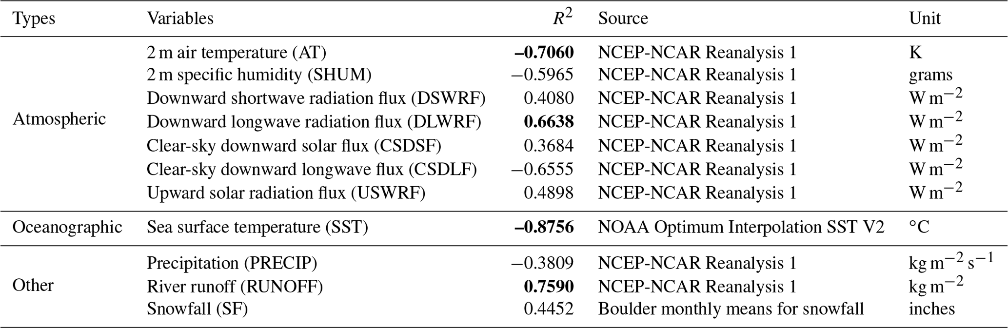
All the sources of dataset used in the IceTFT are listed in Table 1. Except for SST and SF, other data are from the National Centers for Environmental Prediction–National Center for Atmospheric Research (NCEP-NCAR) Reanalysis 1 dataset (Kalnay et al., 1996). To explore whether the model depends on the dataset, we also used another reanalysis dataset to compare. We replaced the data from the NCEP-NCAR Reanalysis 1 with Japanese 55-year Reanalysis (JRA-55; Japan Meteorological Agency, 2013). The results of correlation coefficients with the JRA-55 dataset are similar and not shown in Table 1. The SST data are from the Optimum Interpolation SST V2 data (B. Huang et al., 2001; Reynolds et al., 2007), which is provided by the NOAA National Centers for Environmental Information (NCEI). The SF data are from the Boulder monthly means for snowfall (National Oceanic and Atmospheric Administration Physical Sciences Laboratory, Boulder Climate and Weather Information, 2022).

4 Evaluation metrics

There are three metrics used to evaluate the model performance, namely mean absolute error (MAE), root mean square error (RMSE), and root mean square deviation (RMSD), and the equations are as follows. In particular, RMSD can be used to further investigate the possible reasons for the discrepancy between the observation and prediction values of the SIE. In the formulas of the metrics, the range of n is from 1 to 12, where y and $\stackrel{\mathrm{̃}}{y}$ mean the SIE observation and prediction, and the subscript i represents ith month ordinal of a year. The RMSD is defined as the average distance between predictions and observations. It includes bias and variance components (Zheng et al., 2021). The first component is the mean bias of standard deviations, and the second can be viewed as the mean variation in the square of the difference between the standard deviations of the predictions and the observation, where the R denotes the correlation coefficient between y and $\stackrel{\mathrm{̃}}{y}$. For all the metrics above, a smaller value means that the model has better performance.

$$\begin{array}{}\text{(2)}& {\displaystyle }\mathrm{MAE}={\displaystyle \frac{\mathrm{1}}{n}}\sum _{i=\mathrm{1}}^n|y_i-\stackrel{\mathrm{̃}}{y_i}|\text{(3)}& {\displaystyle }\mathrm{RMSE}=\sqrt{{\displaystyle \frac{\mathrm{1}}{n}}\sum _{i=\mathrm{1}}^n(y_i-\stackrel{\mathrm{̃}}{y_i}{)}^{\mathrm{2}}}\text{(4)}& {\displaystyle }\begin{array}{rl}& \mathrm{bais}={\left(\mathrm{std}\left(y\right)-\mathrm{std}\left(\stackrel{\mathrm{̃}}{y}\right)\right)}^{\mathrm{2}}\\ & \mathrm{variance}={\displaystyle \frac{\mathrm{1}}{n}}\left(y^{\mathrm{2}}+{\stackrel{\mathrm{̃}}{y}}^{\mathrm{2}}-\mathrm{2}y\stackrel{\mathrm{̃}}{y}R\right)\\ & {\mathrm{RMSD}}^{\mathrm{2}}=\mathrm{bais}+\mathrm{variance}\end{array}\end{array}$$

5 The optimal IceTFT model

5.1 The slicing method of inputs

To explore the optimal slicing method of inputs, we used rolling and alignment slicing methods for comparison. Figure 5a shows the process of rolling. A slice of data consists of 12 time step inputs and 12 time step labels, and the whole length is 24. Using the rolling method to move the sliding window by one time step, we can obtain the next 24 time step slice data values. The experiment with the rolling method is named IceTFT-rolling, while the IceTFT-align experiment uses the alignment method, which is shown in Fig. 5b. The aligned inputs require that the first time step data value is for January in each slice of data. With the rolling method, the model can only learn location information but loses temporal features due to the moving time series during training.

Figure 5 The two slicing methods of inputs.

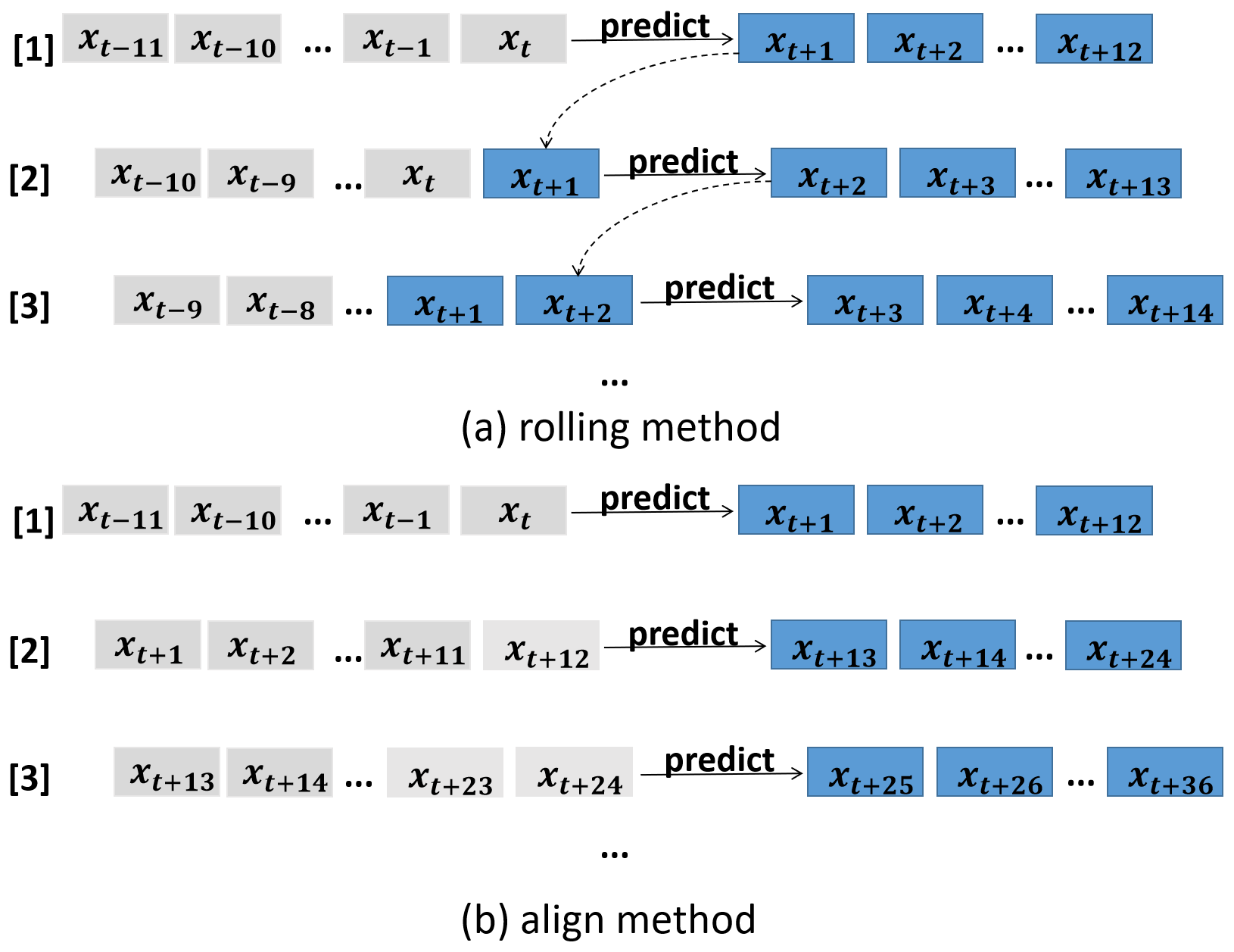
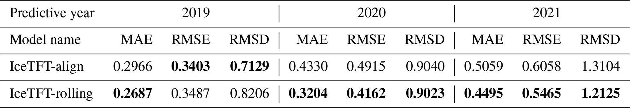
Table 2 shows the prediction results for IceTFT model with different slicing methods. Compared to IceTFT-align and IceTFT-rolling experiments, the IceTFT-align model had a slight advantage from the RMSE and RMSD of 2019, but it had a higher error than the IceTFT-rolling model overall. This may be due to the fact that the IceTFT-align model did not contain a sufficient number of samples for training, so the model cannot learn enough features to predict. It demonstrates that the rolling method is effective with respect to improving the prediction skill. Moreover, it is difficult to predict with high confidence for a model with too few training data points. Therefore, the optimal slicing method of inputs is the rolling method.

Table 2 The three metrics (MAE, RMSE, and RMSD) among two models, with different slicing methods for SIE predictions during 2019–2021. The smallest prediction errors for each year are shown in bold.

5.2 The input length

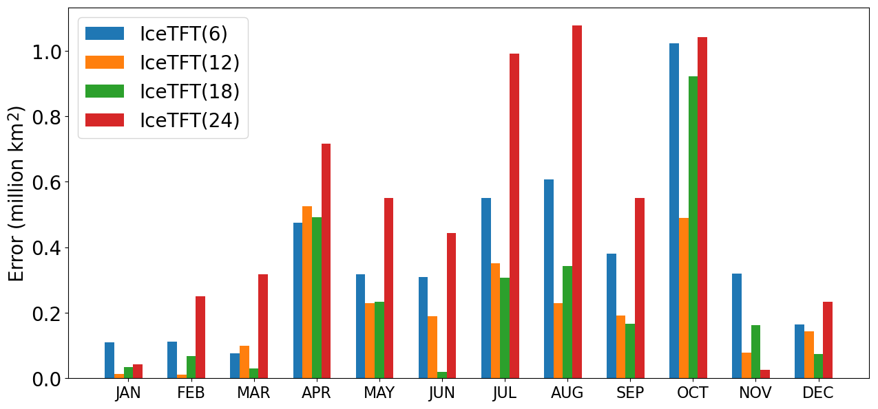
To investigate the effect of the input length on the prediction skill, we chose to set up four sets of comparison experiments with input lengths of $\mathrm{6},\mathrm{12},\mathrm{18}$, and 24. Using the 2019 prediction as an example, the results of the monthly errors are shown in Fig. 6. The results of 2022–2021 are similar and not shown. As a whole, the prediction errors for the models with the input lengths of 6 and 24 are significantly higher than the results for models with other lengths. This is probably because the time window of 6 is too short to include both the March maximum and the September minimum in each epoch. This may affect the model learning for the features of the extremes, thus increasing the inaccuracy of the extremes. However, if the input lengths are too long, then the correlation between the recent historical SIE sequence and the future SIE sequence is weakened, increasing the prediction error. In addition, the errors in a model with 18 months are comparable to a model with 12 months. However, for the difficult prediction of 2019, i.e., in October, which has a large slope, the error in a model with 18 months is significantly higher than one with 12 months. Therefore, for the monthly prediction of SIE, a reasonable choice for the input length is 12 months; it probably is because the period of SIE is 12 months.

Figure 6 The prediction errors in the IceTFT with different input lengths for 2019.

6 The hindcasting experiment results for 2019–2021

Due to the accelerated Arctic SIE decline in recent years with the sparse dataset, many researchers (Chi and Kim, 2017; Kim et al., 2020; Chi et al., 2021) suggest that the recent time period has more useful features than the early period for recent prediction, so they divided more data from the overall dataset to train. We use all the data before the prediction year for training and testing. For example, the IceTFT-2018 model is used to predict SIE from 2019 to 2021, which set the period from 1982 to 2016 as the training data and from 2017 to 2018 as the validation data. IceTFT-2019 and IceTFT-2020 have similar settings, and the details of the settings are shown in Table 3.

Table 3 The sets of training, validation, and prediction for three models.

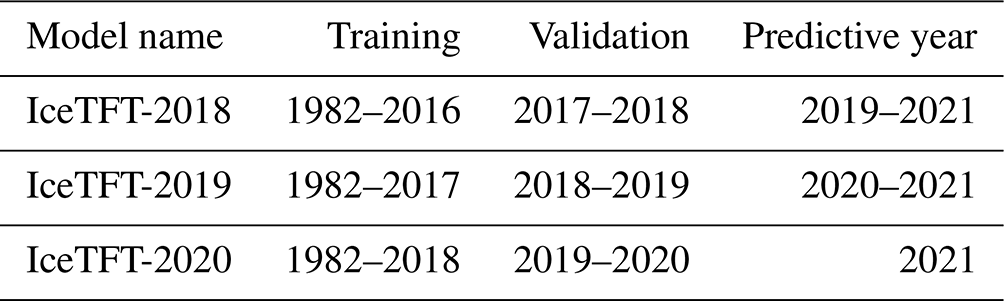
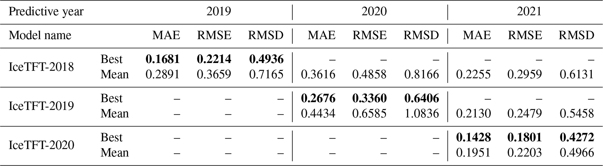
Based on the results in Sect. 5, our later models all use a rolling method to slice the inputs, and the length of the input is chosen to be 12. In this study, we evaluated the prediction skill of the IceTFT by analyzing the results of the hindcast experiment results from 2019 to 2021. Due to the uncertainty in the model, we trained the model 20 times for each of these runs. Then we recorded the best-predicted results and the mean predicted results. The mean predicted results represent the prediction skill of the IceTFT model, while the best-predicted results represent the performance of the IceTFT model with respect to capturing the features of SIE. The results are shown in Table 4.

6.1 Performance of IceTFT for 12-month SIE predictions

From the information in Table 4, it is shown that the models can obtain the predicted results with low error through multiple training. Even though the mean predicted results have a slightly larger error than the best ones, the average predicted error in the model for each month is within 0.3×10⁶ km². In 2019 and 2021, the difference between the best and mean prediction is not significant from the RMSE, which is not more than 0.04×10⁶ km². Compared to the results of these 2 years, the errors in the mean predicted results increased in 2020. This is because there is a second record-low SIE for September 2020. Moreover, due to the predicted period being too long, relatively speaking, evaluating the prediction skill of the IceTFT model using MAE as the loss function is difficult. A low MAE does not mean that the model can predict all 12 months with low errors. The IceTFT model focuses on different physical factors during several training periods and generates predictions with different trends. The model finds it hard to predict this minimum value accurately in each training, so the errors in the mean prediction are much higher than in the best one.

Table 4 The three metrics (MAE, RMSE, and RMSD) among three models for SIE predictions in 2019–2021. The smallest prediction errors for each year are shown in bold.

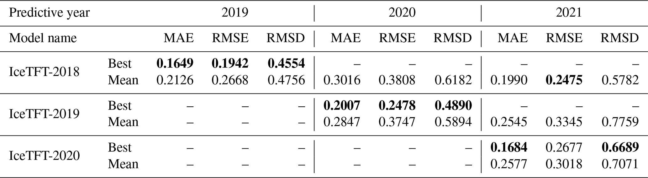
The IceTFT-2019 model had 1 year more training data available than the IceTFT-2018 model, and that caused the model to learn some features of recent times. Consequently, the IceTFT-2019 model has a lower error than the IceTFT-2018 model for 2020 prediction, and the IceTFT-2020 model has a lower error than the IceTFT-2019 model for 2021. These results show that the training data that are closer to the prediction time are more useful than other data that are further away from the moment of prediction. Interestingly, the IceTFT-2018 model also had a higher accuracy for the 2021 prediction. It may be that the trends of SIE between these 2 years are similar (we discussed the reason in Sect. 8). According to the results in Table 4, the RMSE is slightly higher than the MAE for these experiments. The RMSE is more susceptible to outlier influence than MAE. This illustrates that the model with optimal experimental settings produces 25 % mean error (monthly at most) from the MAE but generates a higher error in some months from the RMSE.

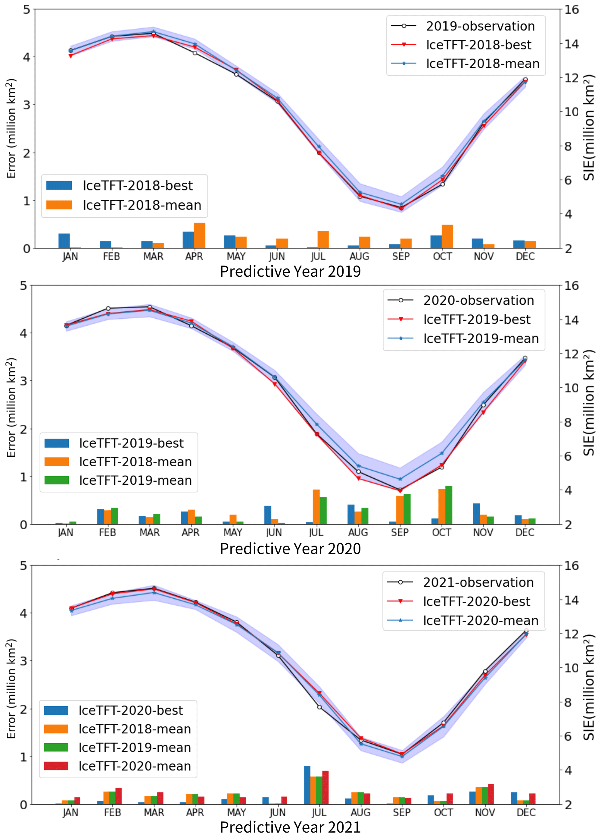
Figure 7 The SIE predictions, observations, and the monthly errors for 2019–2021. The line graph represents the observations and SIE predictions, corresponding to the y axis on the right; the bar graph represents the errors, corresponding to the y axis on the left.

From the bar graphs in Fig. 7, there is a clear trend of predictions for different years, and it also shows the monthly errors. As can be seen, the predictions of multiple training sequences form a prediction period in which the vast majority of observations fall within the range. Except for September 2020, the mean predicted results have the same trend as the observations. In terms of the monthly error in the model with different settings, all of the experiment runs had high errors in October or November. In addition, they had another high error in July, except for 2019. Due to global warming, it is a challenge to predict SIE in summer. In the melt season, which is from June to September, the SIE continued to decline, with a steep slope. The line passing through the observed value of SIE in June and July has the steepest slope. It demonstrates that the SIE reduced significantly from June to July. Thus, it is difficult to predict the downturn. And as a result, the July prediction is higher than the observation with a higher error. The SIE archive is at a minimum in September, and sea ice becomes frozen after that time. Similarly, as with a temperature anomaly or another climate effect, the October or November prediction is on the high side. For 2021 predictions in Fig. 7c, the errors in the IceTFT-2018 model are smaller than the IceTFT-2020 model in the winter but higher in the summer. Though the IceTFT-2018 model has more accuracy than the IceTFT-2020 model from three metrics, it produces more error in September. As a result, the metric is not merely a performance benchmark for prediction. In addition, the monthly errors did not show a monotonically increasing trend, and they did not become greater as the time step increased. The model used a direct predicted method to avoid the superimposition of errors in the recursive approach, and it improved the accuracy of the predictions. The same disadvantage exists for dynamic models, in the sense that the predicted error increases with an increasing prediction period. This issue was resolved by the IceTFT model, which generated longer-term predictions with smaller errors.

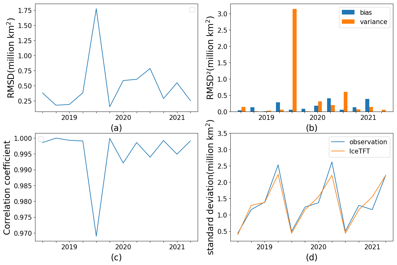
Figure 8 Time series of the RMSD between the detrended quarterly SIE on the IceTFT-model over the period 2019–2021. (a) RMSD; (b) squared RMSD (histogram), consisting of bias and variance; (c) correlation coefficient between predictions and observations; and (d) standard deviation of predictions (orange line) and observations (blue line).

To further explore the potential causes for the inaccuracy, we calculated the RMSD between the detrended quarterly SIE observations and the predictions for the 2019–2021 period. The results are shown in Fig. 8. The RMSD ranges from 0.076 to 0.918 ×10⁶ km² in Fig. 8a, and the findings from the 3 years show a wide spread in the RMSD for each quarter. Figure 8b displays a histogram of the temporal variation in the squared RMSD, which consists of bias and variance, according to Eq. (4). It can be seen that there is a very large variance in the spring (January–March or JFM) of 2020 and 2021, which is responsible for the high RMSD in this season. The correlation coefficients in Fig. 8c also display an obvious reduction in spring 2020, which is consistent with the variations in the variance in Fig. 8b. This result indicates that the significantly lower correlation coefficients are partially responsible for the RMSD peak. Moreover, except for a few months, the magnitude of the bias is substantially larger than the variation in Fig. 8b, indicating that the change in bias is the main factor for the increase in RMSD. Figure 8d shows the standard deviations of the predictions of the IceTFT model and observations, and the annual standard deviation represents the amplitude of the seasonal cycle of SIE. The results show that the difference between these 2 standard deviations is obviously increasing, which contributes to the larger increase in bias over the same period. Furthermore, this is consistent with the finding in Fig. 7. The IceTFT has large model errors when the SIE trend is more volatile (i.e., when the slope is larger), such as in July and October. The biases are larger for the season containing these 2 months. This suggests that IceTFT does not fully capture the signals from the historical data and does not reflect the seasonal variability in the SIE. Thus, we can improve the predictive model by focusing on the seasonal variability in the predictions to reduce the RMSD.

6.2 Comparisons with SIO

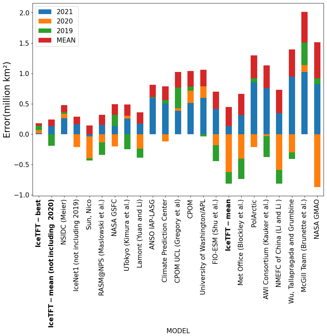
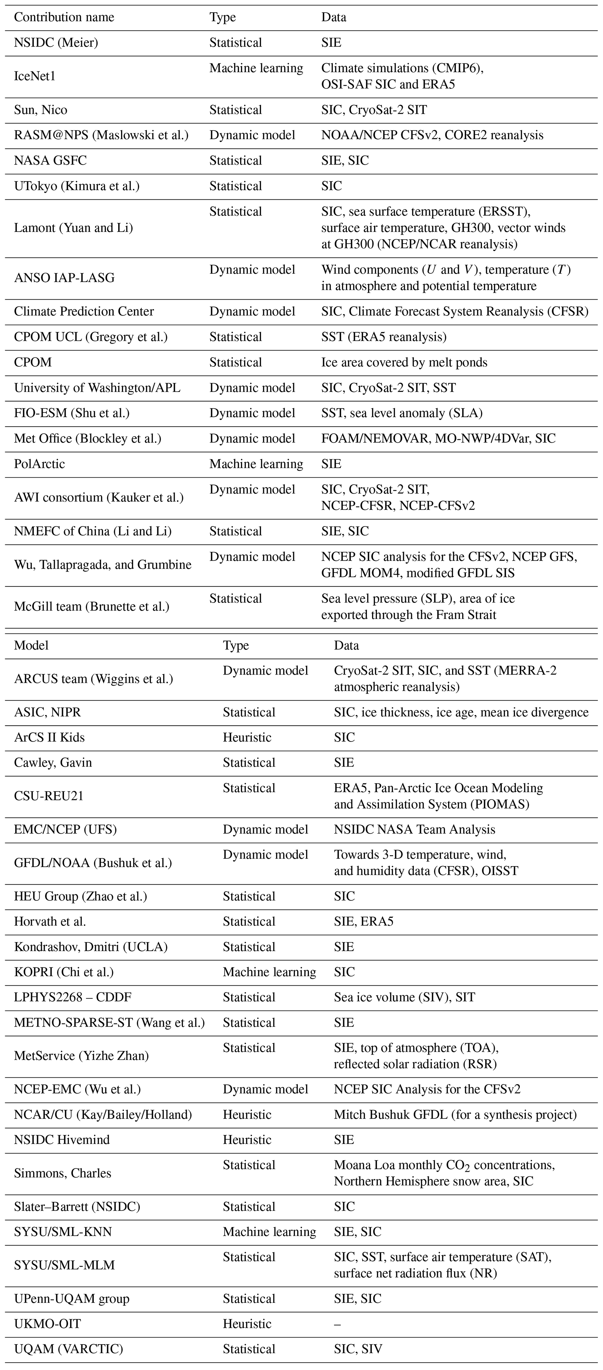
We evaluated the performance of the IceTFT model for the September prediction, in terms of the hindcasting experiments and actual prediction experiments, and collected the contributions submitted to SIO in recent years. For the hindcasting experiments, Fig. 9 presents the errors in September in different models from 2019 to 2021. The types and the data used in the SIO contributions are listed in Appendix A. Compared to the other models, the IceTFT model has the lowest error in prediction over the 3 years. Machine learning always leads to a lower error after repeated training in hindcasting experiments. As can be seen, the best results of the IceTFT model have the smallest errors, but the errors increased a lot in the mean results. The mean prediction indicates that the prediction skill of the model is relatively stable. In addition to 2020, the mean prediction of the IceTFT model is superior to the other models. To make a small error for an anomalous minimum in the mean prediction, the model must have a lower bound for its predictions during the multiple training processes. This is challenging to achieve, as the model is limited by the historical SIE data. Furthermore, the errors in all models are smaller, relative to 2019 (green histogram in Fig. 9). The September observation reached its second-lowest value in 2020, and the anomaly caused the errors to increase (orange histograms are longer than the blue ones). While the extremely low anomalies continue to influence the 2021 predictions, the prediction error in most models has increased (see the blue histogram in Fig. 9). Although the prediction error is greater than that of 2020, the IceTFT model is not influenced by anomalies from the previous year and focuses only on the physical factors that influence the development of sea ice in that year.

Figure 9 The prediction errors in the different contributions in SIO for 2019–2021. These predictions are from the SIO reports (Sea Ice Outlook, 2019a, b, c, 2020a, b, 2021c, a, b, c, d).

6.3 Impacts of datasets on predictions

To investigate whether the prediction results of IceTFT are affected by the source of input data, we replaced the data from the NCEP-NCAR Reanalysis 1 in Table 1 with JRA-55. The same experiments were conducted. Different data sources may be associated with different observation errors, but the physical trends embedded in these data are similar. The IceTFT model can automatically adjust the weights of the input data during the training process by adaptively learning the features, according to the forecast errors. The labeled data with different errors can affect the prediction error calculated by the IceTFT model and thus have a large impact on the prediction skill. Theoretically speaking, the prediction skill of the IceTFT model is limited by the source of the labeled data and does not depend on the source of the input data.

Table 5 The three metrics (MAE, RMSE, and RMSD) among three models with reanalysis datasets for JRA-55 of SIE predictions for 2019–2021. Except for SST and SF, the other inputs were replaced with JRA-55. The smallest prediction errors for each year are shown in bold.

However, the results are shown in Table 5. It can be seen that the best results of the three models are relative to the original results, which are from Table 4, but the mean predictions are higher. This indicates that the models can always obtain optimal predictions after several training epochs in the hindcast experiments and are not limited to the datasets. However, the existence of different observation errors in different datasets makes the bias trends of the predictions different and therefore makes the mean predictions different. Since the prediction errors using NCEP-NCAR Reanalysis 1 are a little smaller, in this paper we still use the original dataset for the experimental analysis.

7 The actual prediction results for 2022

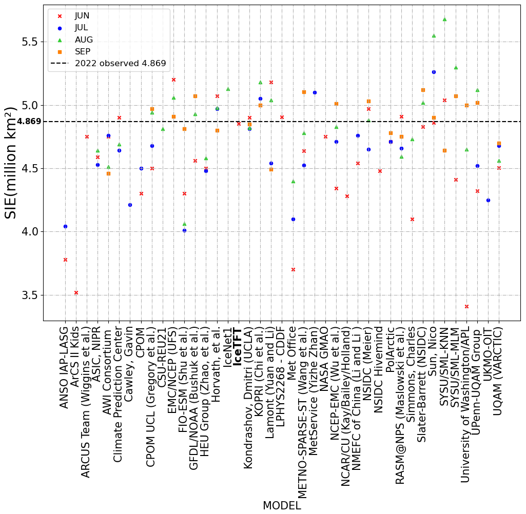
For the actual prediction, we submitted SIPN to the prediction results of the September prediction in June 2022. According to the conclusions in Sect. 6.1, the closer the training set is to the prediction time, the higher skill the model has with respect to prediction. So, we trained the IceTFT-2021 model to predict 2022. As we only use 12 months of data for 2021, and the prediction was 9 months ahead for September, we did not submit a new prediction for July, August, and September as well. Figure 10 shows the 2022 SIE predictions of different models of SIO at different lead times. It can be seen that the prediction results of the different models for 2022 are similar to the findings for the previous 3 years, and their prediction skills do not improve with the reduction in lead time. In particular, the lead time of the contributions in SIO is up to 3 months, but our proposed model has a long lead time of up to 9 months. Compared with the 2022 observed SIE, which is 4.869 ×10⁶ km², the closer predictions are from the IceTFT, LPHYS2268 – CDDF, and Dmitri Kondrashov (UCLA). Interestingly, all three of these contributions are based on statistical models or machine learning methods, where they use SIE instead of SIC to predict SIE directly. This suggests that using SIE to predict SIE has a smaller error than using SIC and can provide a favorable reference for the September prediction. For those contributions based on dynamical models, some of them have larger errors, and their predictions are erratic. For example, the model of Sun Nico performs relatively well when compared to predictions from other dynamical models, but it only submit predictions with small errors in June and September, while there are larger errors in other months. This indicates that the dynamical model has the ability to predict SIE, but there is too much uncertainty, leading to unstable predictions. As can be seen from Figs. 9 and 10, our proposed model has higher a prediction skill than the other models, in both hindcast experiments and real predictions, and it obtains smaller prediction errors with longer lead times.

Figure 10 The predictions of models from SIO for the June, July, August, and September estimates of the September 2022 SIE. These predictions are from the SIO reports (Sea Ice Outlook, 2022a, b, c, d).

8 Interpretability analysis

8.1 Sensitivity experiments

To investigate the contribution of different variables to SIE prediction in the model, we examined the variable sensitivity for different prediction times, which is from 2019 to 2021. Kim et al. (2020) added random Gaussian noises to inputs and calculated the change in RMSE to evaluate the variable sensitivity. In this study, we apply this method to compare the contributions of variables. The equation of IceTFT can be expanded and simply expressed as Eq. (5), where x_i represents the input variables, w_i is the weight of the corresponding variable, and $\widehat{\mathit{\theta }}$ values represent the trainable parameter rather than the weights. We add random Gaussian noises with a 0 mean and 1 standard deviation to each variable, which, in turn, can make some changes in the prediction (Eq. 6). Then we calculate the new RMSE of the model with new inputs and compare the changes in the RMSE (Eq. 7) in scenarios where SIE is the observation. Generally speaking, the sensitivity is greater than 1, which means that the variable plus noise increases the predicted error. However, when the sensitivity is less than 1, it indicates that the change in the variable enhances the accuracy of the predictions. This may be because there is uncertainty in the original data, and the extra noise corrects the data in a beneficial direction for prediction. These particular cases can give us new ideas for improving the prediction skill. To maintain the same range for all of the data, values that are less than 1 are taken as the inverse and marked with a negative sign. Due to the existence of multiple variables interacting with each other, it is difficult to analyze their contribution to the prediction. Therefore, this paper only investigates the sensitivity of the univariate variables.

$$\begin{array}{}\text{(5)}& {\displaystyle }\widehat{\mathrm{SIE}}=F_{\widehat{\mathit{\theta }}}(w_{\mathrm{1}}{x}_{\mathrm{1}},\mathrm{\dots },w_i{x}_i,\mathrm{\dots },w_n{x}_n)\text{(6)}& {\displaystyle }\begin{array}{rl}\widehat{\mathrm{SIE}}+\mathrm{\Delta }{\mathrm{SIE}}_i& =F_{\widehat{\mathit{\theta }}}(w_{\mathrm{1}}{x}_{\mathrm{1}},\mathrm{\dots },w_i{x}_i+\mathrm{\Delta }{x}_i,\mathrm{\dots },w_n{x}_n),\\ & \mathrm{\Delta }{x}_i\sim N(\mathit{\mu },{\mathit{\sigma }}^{\mathrm{2}}),\mathit{\mu }=\mathrm{0},{\mathit{\sigma }}^{\mathrm{2}}=\mathrm{1}\end{array}\text{(7)}& {\displaystyle }\begin{array}{rl}& \mathrm{Sensitivity}\left({\mathrm{Var}}_x\right)=\\ & \left\{\begin{array}{l}\frac{\mathrm{RMSE}(\widehat{\mathrm{SIE}}+\mathrm{\Delta }{\mathrm{SIE}}_i,\mathrm{SIE})}{\mathrm{RMSE}(\widehat{\mathrm{SIE}},\mathrm{SIE})},\\ \mathrm{RMSE}(\widehat{\mathrm{SIE}}+\mathrm{\Delta }{\mathrm{SIE}}_i,\mathrm{SIE})>\mathrm{RMSE}(\widehat{\mathrm{SIE}},\mathrm{SIE})\\ -\frac{\mathrm{RMSE}(\widehat{\mathrm{SIE}},\mathrm{SIE})}{\mathrm{RMSE}(\widehat{\mathrm{SIE}}+\mathrm{\Delta }{\mathrm{SIE}}_i,\mathrm{SIE})},\\ \mathrm{RMSE}(\widehat{\mathrm{SIE}}+\mathrm{\Delta }{\mathrm{SIE}}_i,\mathrm{SIE})<\mathrm{RMSE}(\widehat{\mathrm{SIE}},\mathrm{SIE})\end{array}\right.\end{array}\end{array}$$

Table 6 The variable sensitivity of 11 variables among three models for 2019–2021 in the 11var experiment. The values with higher sensitivity are shown in bold.

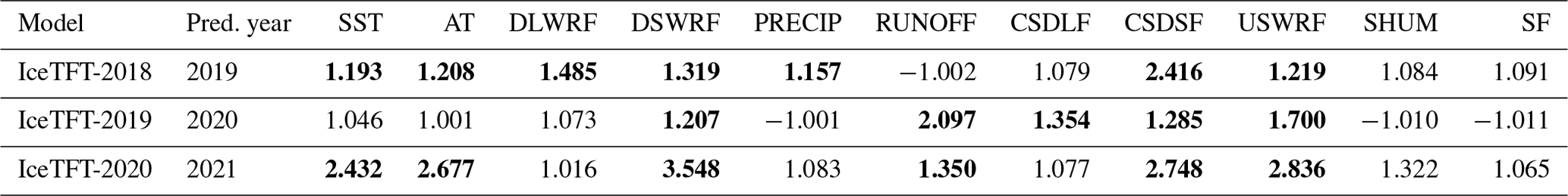
Table 7 The variable sensitivity of six variables among three models for 2019–2021 in the 6var experiment. The values with higher sensitivity are in bold.

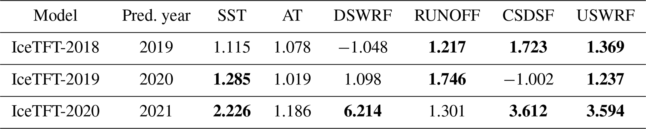
The experiment with 11 variables is denoted as 11var, and the results are shown in Table 6. The values with higher sensitivity are in bold. A higher-sensitivity value indicates that the variable makes a significant contribution to predictions. Multi-variate input of the model may increase the training time and uncertainty. We selected six variables with the highest contributions and redo the same experiments to further investigate the effects of these physical variables on sea ice predictions. These variables include SST, AT, DSWRF, RUNOFF, CSDSF, and USWRF. The experiment with only 6 variables is noted as 6var, and the results of the experiment are shown in Table 7. To analyze the prediction results after reducing the model inputs, we also calculated the difference in the prediction errors between the two experiments, and we plotted the heatmap, as shown in Fig. 11. Negative values are shown in blue, indicating that the 6var experiment has a lower error rate than the 11var. Conversely, the positive values are shown in red, indicating a lower error rate for the 11var experiment with 11 physical factors.

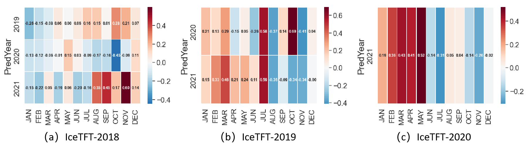
Figure 11 The deviation accuracy between the IceTFT model with six variables (6var) and the IceTFT model with 11 variables (11var) (6var_error−11var_error), with the heatmap values shown within each grid cell. (a) IceTFT-2018 in the 6var experiment, with the deviation accuracy for 3 years, compared to the 11var experiment. (b) IceTFT-2019 in the 6var experiment, with the deviation accuracy relative to that in the 11var experiment for 2 years. (c) IceTFT-2020 in the 6var experiment, with the deviation accuracy compared to that of the 11var experiment.

8.2 Analysis of the physical mechanisms on the years

From the Table 6, we can see that the sensitivity of the predictors is not exactly the same in different years, and the VSN in the IceTFT can automatically adjust their weights to make the model produce an optimal prediction. The variables with a high sensitivity to the predictions are SST, AT, DSWRF, RUNOFF, CSDSF, and USWRF. Most of these variables are related to radiation, and shortwave radiation has a greater impact than longwave radiation. This finding is consistent with other studies in Fig. 4, where surface air temperature and radiative fluxes influence sea surface temperature and thus sea ice melting. While DLWRF is highly correlated in Table 1 but has a low-sensitivity value in Table 6, this indicates that this variable is not the cause of the sea ice change but may be the effect due to the presence of other variables. Other studies have shown that latent heat exchange causes more water vapor and clouds to be present in the atmosphere. This enhances the atmospheric greenhouse effect and results in an increased emission of DLWRF. In addition, the increase in water vapor and clouds will lead to more PRECIP. Therefore, there is a correlation between DLWRF and PRECIP, and their sensitivity values change in agreement, meaning that both have a higher sensitivity in 2019 and are lower in other years. The positive feedback effect, along with the DLWRF, affects the development of sea ice (Kapsch et al., 2016). Since the machine learning model lacks the partial differential equations of the dynamical model, it cannot simulate the variation in the clouds with a positive feedback. Therefore, it is difficult to assist in the SIE prediction, based only on the data trends in DLWRF. While shortwave radiation is influenced by albedo to regulate the effect on sea ice development, the IceTFT model can learn the features of the albedo changes from the historical data. Therefore, the contribution of shortwave radiation in the IceTFT model is larger than that of longwave radiation.

Interestingly, 2020 is a more exceptional year than 2019 and 2021, as it reached the second-lowest value for September on record. SST and AT are less sensitive to 2020 in our experiments. This provides a new idea for investigating the factors affecting the 2020 anomaly. This could be because these 11 variables, which we select, are not the main factors for the unusually small values of 2020. Another reason is that these variables were treated as the monthly mean estimates of global values in the experiments and may have lost their relevance to the Arctic, leading to some impact on the prediction. Other research has shown that the influence on 2020 SIE is primarily caused by the relaxation of the Arctic dipole (Liang et al., 2022). Although it can be seen from our experimental results, neither SST nor AT is a major factor affecting the 2020 SIE prediction, so we will continue to investigate the reasons affecting the SIE anomaly in the future.

8.3 Analysis of the physical mechanisms on the seasons

From Tables 6 and 7, it can be seen that all six variables had a high sensitivity in the 11var experiment, but the sensitivity changed in the 6var experiment. For 2019 prediction in the IceTFT-2018 model, only two of the six variables were relatively sensitive. This indicates that in the 6var experiment, the variable selection networks of IceTFT-2018 model have a greater weighting for the CSDSF and USWRF rather than the SST and AT. These changes cause more errors in summer (June–September or JJAS) and autumn (October–December or OND) but fewer errors in winter (JFM), as can be seen from the first row of Fig. 11a. The most likely explanation is that SST, AT, and other variables from Table 6 has a greater impact on summer and autumn predictions for 2019. And as can be seen from the second row of Fig. 11a, the 6var experiment has fewer errors (almost monthly) for the 2020 predictions. It is also because SST and AT have a lower sensitivity in the 6var experiment, and this conclusion is consistent with the 11var experiment, which suggests that SST and AT may not be the main factors affecting the 2020 predictions. In addition, the impact for 2021 predictions is similar to that for 2019 in the third row of Fig. 11a, and the red areas are darker in autumn and winter. This demonstrates that the factors affecting the 2019 predictions are similar to those for 2021, and SST and AT have a greater impact on 2021 than on 2019. This also validates the experiment results in Fig. 4, explaining that the IceTFT-2018 model had higher accuracy for 2021 predictions.

For the 2020 prediction in IceTFT-2019 model, some of the selected variables were not sensitive to their predictions in the 11var experiment, and the high-sensitivity variables were not fully included. Consequently, their prediction errors have changed significantly in the 6var experiment, according to Fig. 11b. From Table 7, the sensitivity of SST became higher, but that of RUNOFF, DSWRF, and CSDSF decreased in the 6var experiment. According to the first row of Fig. 11b, these changes cause more errors than gains, especially regarding higher errors in winter (JFM), July, and October. This may be due to the fact that the three variables with reduced sensitivity have a greater impact on the 2020 predictions. For the 2021 predictions, the more sensitive SST than for the 11var experiment makes the model in the 6var experiment improve the prediction skill significantly in summer (August–September or AS) and autumn (OND). Compared with those high-sensitivity variables of the IceTFT-2020 model in the 11var experiment from Table 6, AT and other radiation-related variables are not highly weighted in the IceTFT-2019 model for the 6var experiment, with increasing 2021 predicted errors in spring (April–June or AMJ) and winter (JFM), as seen in the second row of Fig. 11b. This indicates that AT and radiation-related variables may have an important impact on 2021 predictions in spring and winter.

Similarly, from the results of Tables 6 and 7, the variables that significantly contributed to the 2021 predictions in the 11var experiment were still selected in the 6var experiment, but the weights of these sensitive variables have also changed. Regarding DSWRF, CSDSF, and USWRF, these radiation-related variables all had high sensitivities for the IceTFT-2020 model in the 6var experiment, and DSWRF is much more sensitive than the other two variables. In comparison to the 11var experiment, these variables had comparable sensitivities. The imbalanced weights led to an increase in the predicted errors in spring (AMJ) and winter (JFM), which are similar to the 2021 predictions in IceTFT-2019 and are shown in Fig. 11b. This suggests that there is some link between these radiation-related variables that collectively affect the prediction skill.

Previous research has demonstrated that sea ice melting is influenced by a complex set of radiative feedback mechanisms (Goosse et al., 2018). Warming Arctic air temperatures cause sea ice to melt, exposing large amounts of the sea surface and thus reducing albedo. The absorption of solar shortwave radiation by the ocean raises sea surface temperatures, which triggers an Arctic amplification effect and creates a positive feedback mechanism that exacerbates the melting of sea ice (Perovich et al., 2007; Screen and Simmonds, 2010). It can be seen that among these processes, AT and SST are the direct factors that influence the melting of sea ice, while longwave radiation and shortwave radiation play an indirect role in this positive feedback mechanism. Consequently, during the melting season, a relatively small area of sea ice cover exposes a large area of sea surface, and warming seawater affects sea ice melt. Since our model cannot simulate the process of radiation absorption by the ocean, SST can provide the IceTFT model with a direct factor affecting the sea ice melt. However, for the freezing season, when the sea ice cover is large and the exposed sea surface area is small, the effect of SST on sea ice melt is relatively small. Instead, heat fluxes and warming air temperatures from water vapor, cloud cover, and radiation mechanisms have a greater effect on sea ice melt (Kapsch et al., 2013; Boisvert and Stroeve, 2015), thus validating the conclusions of our experiments that SST is an important factor influencing the prediction from August to October, while radiation-related variables and AT are at play from January to May.

9 Conclusions

In this study, an interpretable long-term prediction model for the annual predictions of SIE in IceTFT is developed. It uses a total of 11 variables, including atmospheric variables, oceanic variables, and SIE, as inputs to provide relevant mechanisms about the sea ice development process. The IceTFT model can provide the 12-month SIE directly, according to the inputs of the last 12 months, thereby avoiding the need to train multiple models and the error accumulation of iterative prediction. In our experiments, we analyze the effects on the prediction of the slicing methods for input data and the length of input. The results show that the rolling method for slicing data increases the number of datasets, which improves the accuracy of the prediction. Furthermore, the 12-month input includes the whole cycle of SIE, and it is the optimal input length for the prediction. We employ the metrics of MAE, RMSE, and RMSD to evaluate the accuracy of the predictions in the IceTFT model, according to hindcasting experiments from 2019 to 2021 and prediction of 2022. The IceTFT model employs the LSTM encoder, a multi-headed attention mechanism, and a time-static metadata to enhance the learning of the temporal dependence of SIE, so it has a high prediction skill for long-term SIE prediction. In hindcasting experiments, the results show that the monthly average prediction error in the IceTFT model is less than 0.21 ×10⁶ km². For the SIE minimum prediction, compared to other models in SIO with a lead time of 1–3 months, the IceTFT model not only has the smallest prediction error, with a 3-year average SIE minimum prediction error of less than 0.05 ×10⁶ km², but it also provides a 9-month advance prediction. Moreover, we submitted the September prediction to SIO in June 2022, and the IceTFT model has a similarly high prediction skill. Finally, we conducted a sensitivity analysis of the variables to investigate the physical factors that affect the SIE predictions through the VSN design, which can adjust the weights of inputs. The results indicate that the factors affecting the 2020 SIE prediction are different from those of other years. Except for 2020, for the melt season, SST has a greater influence on SIE predictions, while for the freeze season, radiation-related variables have a greater influence than SST. These sensitivities can help researchers investigate the mechanisms of sea ice development, and they also provide useful references for variable selection in data assimilation or the input of deep learning models.

Appendix A: The data used in SIO contributions

Table A1 The data used in SIO (https://www.arcus.org/sipn/sea-ice-outlook, last access: 25 July 2023) contributions. Please note that the predictions and model names have been submitted to the SIO website by different external organizations and/or individuals, and therefore not all references are available for citation.