Simulating heat and CO₂ fluxes in Beijing using SUEWS V2020b: sensitivity to vegetation phenology and maximum conductance

The Surface Urban Energy and Water Balance Scheme (SUEWS) has recently been introduced to include a bottom-up approach to modeling carbon dioxide (CO₂) emissions and uptake in urban areas. In this study, SUEWS is evaluated against the measured eddy covariance (EC) turbulent fluxes of sensible heat (Q_H), latent heat (Q_E), and CO₂ (F_C) in a densely built neighborhood in Beijing. The model sensitivity to maximum conductance (g_max) and leaf area index (LAI) is examined. Site-specific g_max is obtained from observations over local vegetation species, and LAI parameters are extracted by optimization with remotely sensed LAI obtained from a Landsat 7 data product. For the simulation of anthropogenic CO₂ components, local traffic and population data are collected. In the model evaluation, the mismatch between the measurement source area and simulation domain is also considered.

Using the optimized g_max and LAI, the modeling of heat fluxes is noticeably improved, showing higher correlation with observations, lower bias, and more realistic seasonal dynamics of Q_E and Q_H. The effect of the g_max adjustment is more significant than the LAI adjustment. Compared to heat fluxes, the F_C module shows lower sensitivity to the choices of g_max and LAI. This can be explained by the low relative contribution of vegetation to the net F_C in the modeled area. SUEWS successfully reproduces the average diurnal cycle of F_C and annual cumulative sums. Depending on the size of the simulation domain, the modeled annual accumulated F_C ranges from 7.4 to 8.7 $\mathrm{kg}\mathrm{C}{\mathrm{m}}^{-\mathrm{2}}{\mathrm{yr}}^{-\mathrm{1}}$, compared to 7.5 $\mathrm{kg}\mathrm{C}{\mathrm{m}}^{-\mathrm{2}}{\mathrm{yr}}^{-\mathrm{1}}$ observed by EC. Traffic is the dominant CO₂ source, contributing 59 %–70 % to the annual total CO₂ emissions, followed by human metabolism (14 %–18 %), buildings (11 %–14 %), and CO₂ release by vegetation and soil respiration (6 %–10 %). Vegetation photosynthesis offsets only 5 %–10 % of the total CO₂ emissions. We highlight the importance of choosing the optimal LAI parameters and g_max when SUEWS is used to model surface fluxes. The F_C module of SUEWS is a promising tool in quantifying urban CO₂ emissions at the local scale and therefore assisting in mitigating urban CO₂ emissions.

1 Introduction

Currently, half of the global population resides in urban areas, and this percentage is projected to grow to 68 % by the middle of the 21st century (United Nations Department of Economic and Social Affairs, 2019). Urban expansion has reshaped the morphological, thermal, and dynamical properties of the land surface (Grimmond and Oke, 2006; Oke, 1995; Zhu et al., 2016). In addition, intensive human activities in urban areas have caused a large quantity of greenhouse gas emissions (Marcotullio et al., 2013; Velasco and Roth, 2010). Both factors have influenced urban climate from micro-scales to regional scales (Johansson and Emmanuel, 2006; Sarangi et al., 2018; Tan et al., 2010). Climatic and environmental risks due to urbanization are frequently reported, such as heat waves, flooding, and air pollution (Qian et al., 2022; Watts et al., 2015). In this context, there is a pressing need to better understand the effects of urbanization on land–atmosphere interaction, preferably in a quantitative way.

Urban land surface models (ULSMs) are widely used to simulate urban land–atmosphere interactions, including the exchanges of energy, water, and CO₂ and hydrological processes (Chen et al., 2011; Masson et al., 2013). The results from the First International Urban Land Surface Model Comparison Project suggested that the most important processes for urban surface energy balance were radiative and vegetation processes (e.g., vegetation fraction, seasonal cycle of vegetation phenology) (Best and Grimmond, 2015; Grimmond et al., 2010; Nordbo et al., 2015). Long-term observations with low vegetation cover (< 30 %) were especially needed to evaluate heat flux simulation, as energy distribution was found to be sensitive in such environments (Best and Grimmond, 2016).

The Surface Urban Energy and Water balance Scheme (SUEWS) is one of the widely tested ULSMs (Järvi et al., 2011, 2014; Ward et al., 2016). SUEWS is designed to run with surface information (e.g., surface cover fractions) and a minimum amount of model forcing data. In recent years, Supy (SUEWS in Python) was developed to allow Python front-end implementation for broader and easier applications (Sun and Grimmond, 2019). SUEWS has demonstrated good performance against hydrological observations and surface flux observations in several cities in Europe, North America, and Asia (Alexander et al., 2016; Ao et al., 2018; Havu et al., 2022a; Järvi et al., 2011; Ward et al., 2016). In SUEWS, the seasonal cycle of vegetation phenology is indicated by leaf area index (LAI). Previous studies made in two UK cities and Shanghai, China, have reported that bias in modeled LAI leads to overestimation or underestimation in Q_E or Q_H (Ao et al., 2018; Ward et al., 2016). They highlighted the importance of having an appropriate seasonal cycle of LAI in SUEWS. Omidvar et al. (2022) proposed a workflow to derive LAI-related parameters for SUEWS, but it was intended for fully vegetated areas located mainly on the outskirts of cities. Apart from LAI, the maximum conductance (g_max) is also critical in scaling the surface conductance (g_s) and therefore the available energy distribution (Ward et al., 2016). However, the impact of LAI-related parameters and g_max on the modeled turbulent fluxes has received insufficient attention in urban areas.

Recently, the module of local-scale CO₂ flux (F_C) was incorporated into SUEWS (Järvi et al., 2019). It was found to give reasonable annual sum, seasonal, and diurnal cycles against observed F_C in Helsinki, Finland, suggesting that the bottom-up CO₂ emission or uptake estimate in SUEWS can be evaluated by observation-based evidence provided by top-down eddy covariance (EC) measurements. Furthermore, SUEWS shows the potential for broader use, such as quantifying the carbon sequestration potential of urban vegetation (Havu et al., 2022a), investigating the spatial variability of CO₂ emission, quantifying the contribution of each emission component (Järvi et al., 2019), and assisting urban CO₂ emission mitigation. However, this module has not yet been evaluated in cities other than Helsinki.

Beijing provides a unique test bed for SUEWS evaluation and application: a megacity with a population of over 21 million and an increasing urbanized area (MHURD, 2018). The older version of SUEWS (V2017b) has been evaluated and applied in Beijing by Kokkonen et al. (2019), showing good model performance against observed heat fluxes. However, good simulation of turbulent flux does not necessarily imply that the sub-models within give accurate estimates, e.g., LAI and radiative components. Correct presentation of these processes is necessary for more advanced applications like the prediction of surface exchanges of energy under future climate scenarios. Besides, the newly developed F_C module has not yet been evaluated in Beijing.

In this paper, we present a comprehensive evaluation of SUEWS V2020b and its ability to simulate surface fluxes of energy and CO₂ in Beijing. The main aims of this study are (1) to evaluate the model performance of SUEWS using different (default and site-specific) vegetation parameters against the turbulent flux (Q_E, Q_H and F_C) measurements and (2) to estimate the contributions of the anthropogenic and biogenic components to the F_C with the bottom-up modeling approach of SUEWS. Meanwhile, the impact of the mismatch between the turbulent flux source area and the modeled area is also examined.

2 Model description

SUEWS is an urban land surface model that simulates the surface energy and water balances and CO₂ flux at a local (neighborhood) scale (Järvi et al., 2011, 2019; Ward et al., 2016). In SUEWS, the modeling domain is separated into seven interacting surface types (buildings, paved surfaces, grass, evergreen trees/shrub, deciduous trees/shrubs, bare soil, and waterbody), with a single soil layer below each type. SUEWS is designed to run with surface information (e.g., surface cover fractions) and a minimal amount of model forcing data, including wind speed (U), relative humidity (RH), air temperature (T_air), air pressure (p), precipitation, and incoming solar radiation (K_down). SUEWS has sub-models for LAI and net all-wave radiation, and users are allowed to modify the parameters of the sub-models based on the information of the modeled domain. In this study, we use SUEWS version V2020b (Havu et al., 2022b).

2.1 Leaf area index model

In SUEWS, leaf growth is accumulated when T_air stays above the limit value $T_{\text{base},\mathrm{GDD},i}$ consecutively, denoted by growing degree day (GDD). Leaf growth is allowed until GDD reaches the upper boundary GDD_full,i or LAI reaches its maximum (LAI_max,i). Similar to the leaf growth period, the leaf-off period is impacted by $T_{\text{base},\mathrm{SDD},i}$, senescence degree day (SDD), and SDD_full,i or LAI_min,i. Leaf fall is controlled by T_air or (at high latitudes) by day length (Järvi et al., 2014). Here, LAI for vegetation type i at the day of year d (LAI_d,i) is defined as follows:

$$\begin{array}{}\text{(1)}& \begin{array}{rl}& {\mathrm{LAI}}_{d,i}=\\ & \left\{\begin{array}{l}\text{min}\left({\mathrm{LAI}}_{\text{max},i},{\mathrm{LAI}}_{d-\mathrm{1},i}^{{\mathit{\omega }}_{\mathrm{1}},\mathrm{GDD},i}\cdot {\mathrm{GDD}}_{d,i}\cdot {\mathit{\omega }}_{\mathrm{2},\mathrm{GDD},i}+{\mathrm{LAI}}_{d-\mathrm{1},i}\right),\\ \mathrm{\text{leaf-on}},T_{\text{base},\mathrm{GDD},i}>T_{d-\mathrm{1}}\\ \text{max}\left({\mathrm{LAI}}_{\text{min},i},{\mathrm{LAI}}_{d-\mathrm{1},i}^{{\mathit{\omega }}_{\mathrm{1}},\mathrm{SDD},i}\cdot {\mathrm{SDD}}_{d,i}\cdot {\mathit{\omega }}_{\mathrm{2},\mathrm{SDD},i}+{\mathrm{LAI}}_{d-\mathrm{1},i}\right),\\ \mathrm{\text{leaf-off}},T_{d-\mathrm{1}}<T_{\text{base},\mathrm{SDD},i},\end{array}\right.\end{array}\end{array}$$

where LAI_max,i and LAI_min,i for each vegetation type can be obtained from literature or determined from observations, ${\mathit{\omega }}_{\mathrm{1}/\mathrm{2},\mathrm{GDD}/\mathrm{SDD},i}$ represents the growing or senescence rates derived for each study site or uses their default values (Järvi et al., 2011; Omidvar et al., 2022), and T_d−1 is the previous day air temperature mean.

2.2 Radiation fluxes

K_down is a required variable in the meteorological forcing data, whereas other radiation components are estimated within SUEWS. Outgoing shortwave radiation (K_up) is calculated using a bulk albedo (α) based on the area fraction for each surface type. Incoming longwave radiation (L_down) is calculated using T_air and RH to estimate the cloud cover and the clear-sky emissivity (Loridan et al., 2011), while outgoing longwave radiation (L_up) is estimated by surface emissivity, α, K_down, L_down, and T_air (Offerle et al., 2003).

2.3 Turbulent heat fluxes

Latent heat flux (Q_E, W m⁻²) is calculated using the modified Penman–Monteith equation for each surface type:

$$\begin{array}{}\text{(2)}& Q_{\mathrm{E}}={\displaystyle \frac{s(Q_{\mathrm{N}}+Q_{\mathrm{F}}-\mathrm{\Delta }{Q}_{\mathrm{s}})+\mathit{\rho }{c}_p\mathrm{VPD}/r_{\text{av}}}{s+\mathit{\gamma }(\mathrm{1}+r_{\mathrm{s}}/r_{\text{av}})}},\end{array}$$

where Q_N (W m⁻²) is the net all-wave radiation, Q_F (W m⁻²) is the anthropogenic heat flux, ΔQ_S (W m⁻²) is the net storage heat flux, ρ (kg m⁻³) is the air density, c_p ($\mathrm{J}{\mathrm{kg}}^{-\mathrm{1}}{\mathrm{K}}^{-\mathrm{1}}$) is the specific heat capacity of air at constant pressure, VPD (Pa) is the vapor pressure deficit, s ($\mathrm{Pa}{}^{\circ }{\mathrm{C}}^{-\mathrm{1}}$) is the slope of the saturation vapor pressure curve, γ ($\mathrm{Pa}{}^{\circ }{\mathrm{C}}^{-\mathrm{1}}$) is the psychrometric constant, r_av (s mm⁻¹) is the aerodynamic resistance for water vapor, and r_s (s mm⁻¹) is the surface resistance. r_s, or its inverse surface conductance g_s (mm s⁻¹), has the following form:

$$\begin{array}{}\text{(3)}& \begin{array}{rl}{g}_{\mathrm{s}}={\displaystyle \frac{\mathrm{1}}{r_{\mathrm{s}}}}=& \sum _i\left(g_{\text{max},i}{\displaystyle \frac{{\mathrm{LAI}}_i}{{\mathrm{LAI}}_{\text{max},i}}}{\mathrm{fr}}_i\right)\\ & \times G_{\mathrm{1}}g\left(K_{\text{down}}\right)g\left(\mathrm{\Delta }q\right)g\left(T_{\text{air}}\right)g\left(\mathrm{\Delta }\mathit{\theta }\right),\end{array}\end{array}$$

where g_max,i is the maximum conductance of vegetation type i; fr_i is the surface fraction of i; G₁ is a constant connecting stomatal conductance to canopy conductance; and g(K_down), g(Δq), g(T_air), and g(Δθ) are environmental response functions on K_down, specific humidity deficit (Δq), air temperature (T_air), and soil moisture deficit (Δθ), respectively. The functions have the following forms (Ward et al., 2016):

$$\begin{array}{}\text{(4)}& {\displaystyle }g\left(K_{\text{down}}\right)={\displaystyle \frac{K_{\text{down}}/(G_{\mathrm{2}}+K_{\text{down}})}{K_{\text{down},\text{max}}/(G_{\mathrm{2}}+K_{\text{down},\text{max}})}},\text{(5)}& {\displaystyle }g\left(\mathrm{\Delta }q\right)=G_{\mathrm{3}}+(\mathrm{1}-G_{\mathrm{3}})G_{\mathrm{4}}^{\mathrm{\Delta }q},\text{(6)}& {\displaystyle }g\left(T_{\text{air}}\right)={\displaystyle \frac{(T_{\text{air}}-T_{\mathrm{L}})(T_{\mathrm{H}}-T_{\text{air}}{)}^{T_{\mathrm{C}}}}{(G_{\mathrm{5}}-T_{\mathrm{L}})(T_{\mathrm{H}}-G_{\mathrm{5}}{)}^{T_{\mathrm{C}}}}},\end{array}$$

where

$$\begin{array}{}\text{(7)}& T_{\mathrm{C}}={\displaystyle \frac{(T_{\mathrm{H}}-G_{\mathrm{5}})}{(G_{\mathrm{5}}-T_{\mathrm{L}})}},\end{array}$$

and

$$\begin{array}{}\text{(8)}& g\left(\mathrm{\Delta }\mathit{\theta }\right)={\displaystyle \frac{\mathrm{1}-\text{exp}\left(G_{\mathrm{6}}\right(\mathrm{\Delta }\mathit{\theta }-\mathrm{\Delta }{\mathit{\theta }}_{\text{WP}}\left)\right)}{\mathrm{1}-\text{exp}(-G_{\mathrm{6}}\mathrm{\Delta }{\mathit{\theta }}_{\text{WP}})}}.\end{array}$$

Coefficients G₂–G₆ determine the shape of the curves describing responses of stomatal conductance to each environmental variable. K_down,max (W m⁻²) is the maximum incoming solar radiation; T_L and T_H (^∘C) are the lower and upper limits for temperature at which photosynthesis and transpiration are off, respectively; and Δθ_WP (mm) is wilting point deficit. K_down (W m⁻²) is model input, Δq (g kg⁻¹) is calculated from model input RH, T_air (^∘C) is either model input or simulated at 2 m height, and Δθ (mm) is simulated within SUEWS (Järvi et al., 2017). Q_H is determined as the residual from the surface energy balance equation:

$$\begin{array}{}\text{(9)}& Q_{\mathrm{H}}=Q_{\mathrm{N}}+Q_{\mathrm{F}}-\mathrm{\Delta }{Q}_{\mathrm{S}}-Q_{\mathrm{E}}.\end{array}$$

2.4 CO₂ flux

The F_C module adopts a bottom-up approach to determine the local-scale F_C ($\mathrm{\mu }\mathrm{mol}{\mathrm{m}}^{-\mathrm{2}}{\mathrm{s}}^{-\mathrm{1}}$), accounting for both anthropogenic (F_C,ant) and biogenic (F_C,bio) components (Järvi et al., 2019):

$$\begin{array}{}\text{(10)}& \begin{array}{rl}{F}_{\mathrm{C}}& =F_{\mathrm{C},\text{ant}}+F_{\mathrm{C},\text{bio}}\\ & =(F_{\mathrm{M}}+F_{\mathrm{V}}+F_{\mathrm{B}}+F_{\mathrm{P}})+(F_{\text{pho}}+F_{\text{res}})\end{array}.\end{array}$$

In Eq. (10), F_M is the CO₂ emissions from human metabolism, F_V is the emissions from traffic, F_B is the emissions from buildings (e.g., combustion of natural gas, coal, and wood), F_P is the emissions from local-scale point sources, F_pho is the CO₂ uptake by photosynthesis, and F_res is the CO₂ release by soil and vegetation respiration. Positive values indicate CO₂ emissions, and negative values indicate CO₂ uptake with respect to the atmosphere. F_pho has a negative sign, while the rest of the F_C components have a positive sign.

F_C,ant relates to the energy balance through Q_F. F_M and F_V are estimated with an inventory approach, i.e., based on population density or traffic rate, and their emission factors (EFs). Hourly CO₂ emissions from human metabolism on weekdays or weekends ($F_{\mathrm{M},\mathrm{h},\mathrm{d}}$, $\mathrm{\mu }\mathrm{mol}{\mathrm{m}}^{-\mathrm{2}}{\mathrm{s}}^{-\mathrm{1}}$) are calculated using

$$\begin{array}{}\text{(11)}& F_{\mathrm{M},\mathrm{h},\mathrm{d}}=p_{\mathrm{d}}\cdot {\mathrm{PP}}_{\mathrm{h},\mathrm{d}}\cdot {\mathrm{AP}}_{\mathrm{h},\mathrm{d}}\cdot C_{\mathrm{M}},\end{array}$$

where p_d is the daily average population density (cap ha⁻¹), PP_h,d is the population diurnal profile by hour, AP_h,d is the activity level diurnal profile by hour, and C_M is the CO₂ release per person (µmol CO₂ s⁻¹ per capita). The p_d and PP_h,d reconstruct the diurnal population density cycle. AP_h,d scales the C_M to vary between the nighttime minimum and daytime maximum values (C_M(min,max)) to indicate the diurnal cycle of per capita human metabolic intensity.

Hourly traffic CO₂ emissions ($F_{\mathrm{V},\mathrm{h},\mathrm{d}}$) on weekdays or weekends are calculated from

$$\begin{array}{}\text{(12)}& F_{\mathrm{V},\mathrm{h},\mathrm{d}}={\mathrm{Tr}}_{\mathrm{d}}\cdot E_{\mathrm{c},\mathrm{d}}\cdot H_{\mathrm{T},\mathrm{d}},\end{array}$$

where Tr_d is the mean daily traffic rate within the study area ($\mathrm{veh}{\mathrm{d}}^{-\mathrm{1}}{\mathrm{area}}^{-\mathrm{1}}$), H_T,d is the diurnal traffic profile, and E_c,d is the traffic EFs for CO₂ (kg km⁻¹ per vehicle).

Hourly building CO₂ emissions ($F_{\mathrm{B},\mathrm{h},\mathrm{d}}$) on weekdays or weekends are calculated from

$$\begin{array}{}\text{(13)}& \begin{array}{rl}{F}_{\mathrm{B},\mathrm{h},\mathrm{d}}=& [{\mathrm{fr}}_{\text{heat}}\cdot Q_{\mathrm{F},\text{heat}}+{\mathrm{fr}}_{\text{nonheat}}\cdot Q_{\mathrm{F},\text{base}}\cdot {\mathrm{fr}}_{\text{QF},\text{base},\mathrm{BEU},\mathrm{d}}]\\ & \times E_{{\mathrm{CO}}_{\mathrm{2}}\text{ per J}},\end{array}\end{array}$$

where fr_heat is the fraction of fossil fuels used for heating; Q_F,heat is the building heat emission at local scale estimated from the heating degree day model (Järvi et al., 2011); fr_nonheat is the fraction of fossil fuels used for energy other than heating (e.g., the use of gas stove for cooking); Q_F,base is the non-temperature-related anthropogenic heat flux (W m⁻²) including heat emissions from traffic, human metabolism, and electricity usage; ${\mathrm{fr}}_{\text{QF},\text{base},\mathrm{BEU},\mathrm{d}}$ is the fraction of the Q_F,base coming from building energy use on weekdays or weekends; and $E_{{\mathrm{CO}}_{\mathrm{2}}\text{ per J}}$ is the EF for fuels in building energy use (µmol CO₂ J⁻¹). Emissions from single-point sources such as power plants and industrial activities can be included as model inputs.

F_pho relates to the energy balance through LAI and the environmental responses of surface conductance (Eq. 3). F_pho is calculated using

$$\begin{array}{}\text{(14)}& \begin{array}{rl}{F}_{\text{pho}}=& \sum _i\left({\mathrm{fr}}_i{F}_{\text{pho},\text{max},i}{\mathrm{LAI}}_i\right)\\ & \times g\left(T_{\text{air}}\right)g\left(\mathrm{\Delta }q\right)g\left(\mathrm{\Delta }\mathit{\theta }\right)g\left(K_{\text{down}}\right),\end{array}\end{array}$$

where $F_{\text{pho},\text{max},i}$ is the maximum photosynthetic rate for vegetation type i.

Soil and vegetation respiration F_res ($\mathrm{\mu }\mathrm{mol}{\mathrm{m}}^{-\mathrm{2}}{\mathrm{s}}^{-\mathrm{1}}$) follows an exponential dependency on T_air:

$$\begin{array}{}\text{(15)}& F_{\text{res}}=\sum _i{\mathrm{fr}}_i\text{max}(a_i\cdot \text{exp}(T_{\text{air}}{b}_i),\mathrm{0.6}),\end{array}$$

where a_i and b_i are the parameters controlling the temperature dependency and 0.6 $\mathrm{\mu }\mathrm{mol}{\mathrm{m}}^{-\mathrm{2}}{\mathrm{s}}^{-\mathrm{1}}$ is the minimum respiration in winter time.

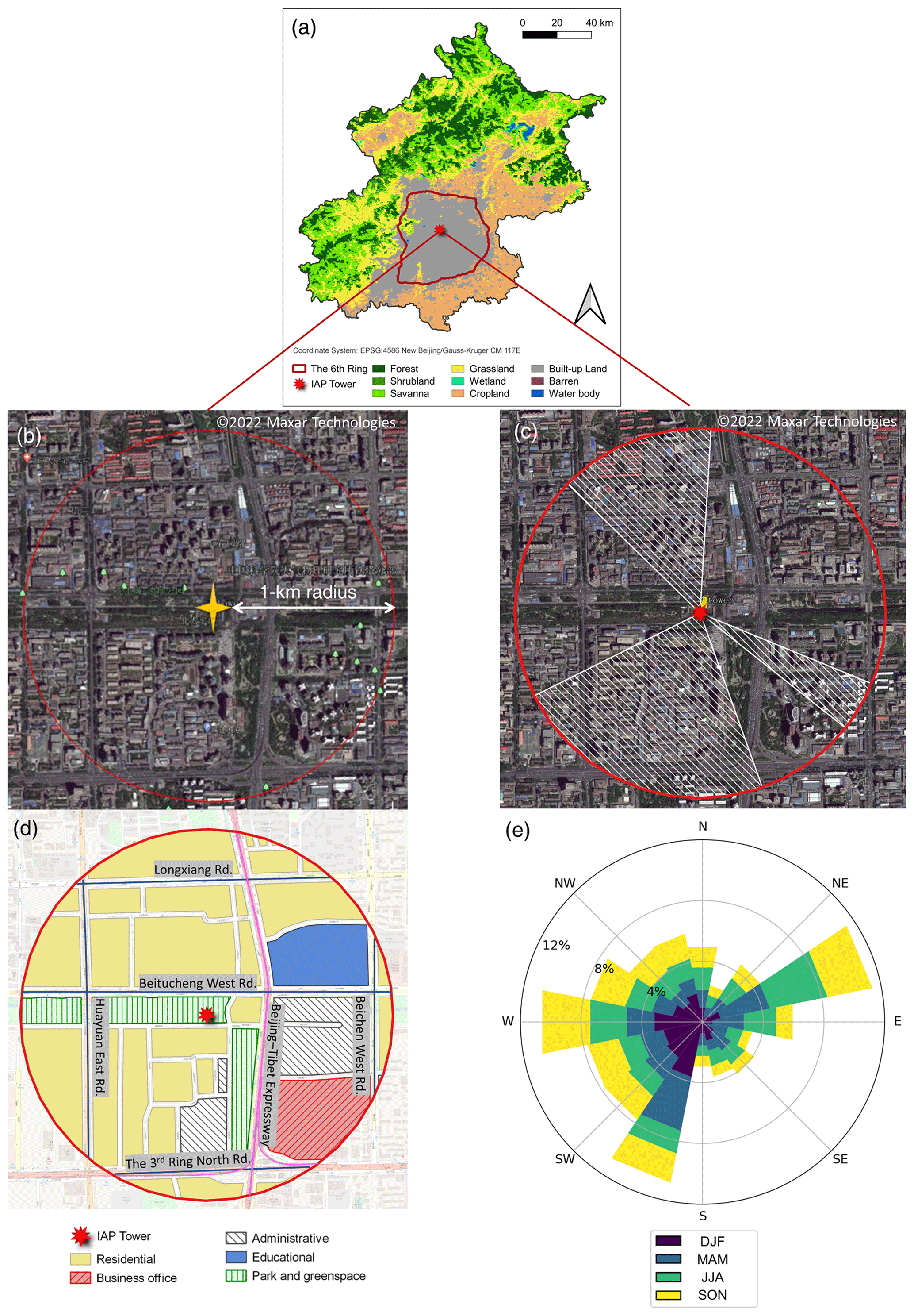
Figure 1 (a) The location of IAP tower and the land cover type within the 6th Ring Road area of Beijing (MODIS land cover type (MCD12Q1) version 6; Friedl and Sulla-Menashe, 2019). (b) A satellite image (Google Earth, image ©2022 Maxar Technologies) over the study area. (c) Wind sectors that have been filtered out for data quality control. (d) Urban land use categories (EULUC-China) (Gong et al., 2020). (e) Wind direction frequency by season.

3 Study site and measurements

The model domain is a 1 km circle around the 325 m meteorological tower constructed by Institute of Atmospheric Physics, Chinese Academy of Sciences (IAP tower, 39^∘58^′ N, 116^∘22^′ E, 60 m above sea level) located in the 6th Ring Road area of Beijing, China (Fig. 1a–d). An EC setup at the height of 47 m on IAP tower continuously measures the surface fluxes of Q_E, Q_H and F_C using a three-dimensional sonic anemometer (Windmaster, Gill, UK) and an open-path infrared gas analyzer (LI-7500A, LI-COR, USA). In addition, all four radiation components are measured at the height of 140 m using a net radiometer (CNR1, Kipp & Zonen, Netherlands). These measurements are used to evaluate SUEWS model performance. The 1 km radius circle around IAP tower roughly covers 80 % of the accumulated flux footprint area (Liu et al., 2012). This area is mainly covered by impervious surfaces (Fig. 1b). Three patches of urban green spaces are situated to the east, south, and west to IAP tower, while the other vegetation is sparsely spread along the roads and near the buildings. Most of the impervious surfaces in the source area are residential buildings (Fig. 1d). A more detailed description of the surroundings and the used instruments can be found in previous publications by Cheng et al. (2018), Liu et al. (2012), and Liu et al. (2021).

The 30 min turbulent flux calculation procedures and the quality controls were described in detail by Cheng et al. (2018). Quality controls such as out-of-limit value removal, spike removal, and a dropout test were conducted on the 10 Hz data during the flux calculation. In order to exclude low-quality data caused by precipitation, dust, or other contamination on the sensor, the records with automatic gain control value ≥ 62 were discarded. On top of the procedures by Cheng et al. (2018), the following quality control steps are performed for 30 min turbulent flux observations in the year 2016. (1) Upper- and lower-boundary filtering is performed to remove observations that fall outside specified ranges: Q_E from −500 to 1000 W m⁻², Q_H from −500 to 1000 W m⁻², and F_C from −100 to 200 $\mathrm{\mu }\mathrm{mol}{\mathrm{m}}^{-\mathrm{2}}{\mathrm{s}}^{-\mathrm{1}}$. (2) Spike detection is done to remove flux values outside 3.5 standard deviations of the 3 d moving mean value (Liu et al., 2012). (3) Wind direction filtering is performed to remove the wind directions with building heights over 50 m (112–128, 160–243, 314–3^∘) (Kokkonen et al., 2019) (Fig. 1c). (4) Stationarity tests are performed to filter out data points with stationary indicator > 30 % (Foken and Wichura, 1996). The percentage of data removed through these four steps is 0.2 %–0.3 %, 1.7 %–2.7 %, 37.8 %–38.2 %, and 13.1 %–17.4 %, respectively. The numbers of observations retained after quality control are 8017 for Q_E, 7338 for Q_H, and 7797 for F_C. These 30 min flux observations are resampled to 1 h resolution. In addition, F_C is gap-filled using seasonal mean diurnal cycle in order to calculate the seasonal and annual sums (Falge et al., 2001).

Wind directions are mainly from the southern and western sectors and the northeastern and eastern sectors before the implementation of the wind direction filtering (Fig. 1 e). In winter, wind from the west is more frequently seen than from the east compared to the other seasons.

To optimize the behavior of LAI, a 6-year time series (2011–2016) of LAI over an adjacent park near the IAP tower is calculated from the atmospherically corrected surface reflectance provided by the USGS Landsat 7 Enhanced Thematic Mapper + (ETM+) (30 m spatial resolution) via the Google Earth Engine Data Catalog (Masek et al., 2006). The atmospherically corrected surface reflectance bands have been preprocessed using the scaling factors from the metadata. Next, enhanced vegetation index (EVI) is calculated using the following formula (Huete, 1997):

$$\begin{array}{}\text{(16)}& \begin{array}{rl}\mathrm{EVI}=& \mathrm{2.5}\times (\mathrm{NIR}-\mathrm{RED})/\\ & (\mathrm{NIR}+\mathrm{6}\times \mathrm{RED}-\mathrm{7.5}\times \mathrm{BLUE}+\mathrm{1}),\end{array}\end{array}$$

where NIR, RED, and BLUE are the near-infrared, red, and blue bands, respectively. EVI is further used to calculate LAI with the formula (Boegh et al., 2002):

$$\begin{array}{}\text{(17)}& \mathrm{LAI}=\mathrm{3.618}\times \mathrm{EVI}-\mathrm{0.118}.\end{array}$$

The LAI and air temperature time series are subjected to optimization using the covariance matrix adaptation evolution strategy (CMA-ES) (Appendix A). Before the optimization process, values larger than 10 m² m⁻² and negative values are considered outliers and removed; values during December and January are set to a fixed value, i.e., the average of these months (0.2 m² m⁻²), to reduce the noise in winter and improve optimization performance. More details can be found in Appendix A. The related data and code are openly available to reproduce the results (Zheng et al., 2022).

4 Model run

4.1 Forcing meteorological data

The reanalysis dataset WFDE5 (Cucchi et al., 2021) is used as the forcing data for SUEWS. WFDE5 is a bias-corrected dataset of near-surface meteorological variables specifically suited for land surface modeling. It is derived from the fifth generation of the European Centre for Medium-Range Weather Forecasts (ECMWF) atmospheric reanalysis (Hersbach et al., 2020). It is provided at 0.5^∘ spatial resolution and at hourly temporal resolution. WFDE5 is evaluated against observed meteorological observations before it is used as the forcing data for SUEWS (Appendix B).

4.2 Land cover

Land cover types and their fractions needed in the model cases are estimated based on aerial images. Paved surfaces account for 46 % of the total area, buildings 24 %, trees/shrub 13 %, grass/lawn 16 %, and water 1 %. The average building height is 19.1 m (Kokkonen et al., 2019). According to a field survey conducted in the 6th Ring Road area, the population of deciduous species accounts for 82 % of the total number of woody plants investigated (Ma, 2019). Therefore, the surface fraction of deciduous trees is set to 11 % and evergreen trees 2 %.

Due to the wind direction filtering (Sect. 3), the actual flux source area “seen” by the EC measurement is biased from the 1 km radius circle around IAP tower. The vegetation fraction is 31 % in the remaining sectors combined, as compared to 29 % in the entire 1 km radius circle (Fig. 1b–c, Table S1 in the Supplement). The model performance in turbulent flux modeling with the land fractions for the remaining sectors is similar to the entire circle (Fig. S1 in the Supplement). Therefore, only the results using the land fractions of the entire circle are demonstrated in the main text.

4.3 Storage heat flux

To calculate the storage heat flux, the Objective Hysteresis Model (OHM) is used (Grimmond and Oke, 1999). The coefficients for all the surface types follow the previous study by Kokkonen et al. (2019). A large portion of the paved surface is asphalt in the study area. Thus, the coefficients are set to the weighted average values of asphalt surface (AN99) following Ward et al. (2016).

4.4 Human activity

In this study, local parameters of traffic, population dynamics, and building energy use are incorporated in order to estimate Q_F and CO₂ emissions.

Ward et al. (2013)Moriwaki and Kanda (2004)Wen et al. (2020, 2022)Zhang et al. (2014)Wen et al. (2020, 2022)Zhang et al. (2014)Yang et al. (2019)Yang et al. (2019)Cui et al. (2019)MHURD (2018)Zhang et al. (2019)BMBS (2017)Cui et al. (2019)

Table 1 Parameters related to anthropogenic heat and CO₂ emissions.

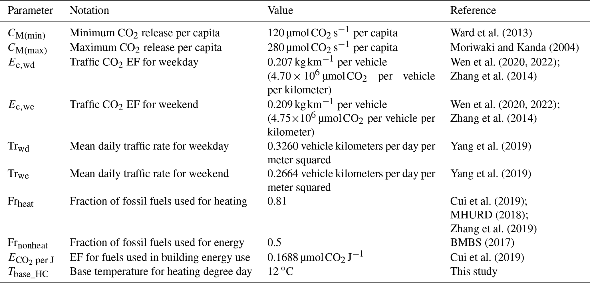
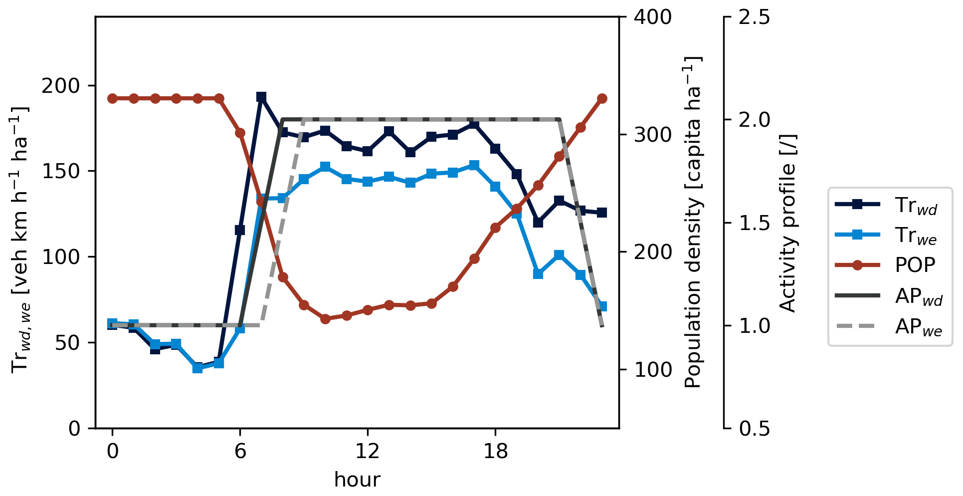
Figure 2 Annual average diurnal cycle of traffic rate for weekday (Tr_wd) and weekend (Tr_we), population density (POP), and the activity profiles for weekdays (AP_wd) and weekend (AP_we) within the 1 km radius circle around IAP tower.

The annual mean weekday and weekend diurnal cycle of traffic rate for each road link in 2017 in the study domain are all extracted from a dataset based on an extensive road traffic monitoring network (Yang et al., 2019). For weekends and weekdays, the diurnal traffic cycles are calculated independently. The total hourly traffic rate (vehicle kilometer per hour) is calculated as the sum of the traffic rates, i.e., the product of traffic volume (vehicles per hour) and the road link length (km) from all the road links in the study area. The hourly traffic rates are then summed up to the total daily traffic rates (vehicle kilometer per day) and divided by the total modeling area, yielding Tr_d. Finally, the diurnal traffic profiles (H_T,d) are obtained by normalizing the diurnal cycles of the total hourly traffic rate (Table 1, Fig. 2).

The annual average diurnal cycle of population density within the model domain is obtained from a dataset of hourly population dynamics at 500 m resolution generated from remotely sensed and geospatial data over the years 2015 and 2016 (Zhao et al., 2021) (Fig. 2). As there are several residential building areas located within the model domain (Fig. 1d), population density increases in the evening when residents get home from work, remains high throughout the night, and decreases in the morning. Weekdays and weekends share the same diurnal cycle of population density in our study.

Heating in Beijing is dominated by central heating, supplied mainly at the district level. The sources include cogeneration plants fueled by coal or gas and district boilers powered by coal, oil, or gas. Cogeneration plants are usually located at suburban or rural areas, and there are no cogeneration plants within the model domain, meaning that their contribution to CO₂ emission is neglected in this study. In comparison, boiler plants are very common: over 5000 coal-fired and 1000 gas-fired heating boilers were located surrounding the populated areas in 2014 (Cui et al., 2019). We investigated the boiler plants near the IAP tower through interviews and found that there were at least 11 of them located at multiple directions within a 1.5 km distance from the IAP tower. For the known boiler plants, eight of them have a chimney height lower than 20 m. Thus, their CO₂ emissions are very likely to be observed by EC at 47 m during the heating season. Unfortunately, the heating capacity and detailed information regarding the fuel combustion for each boiler plant are either unknown or restricted from access. Therefore, it is challenging to treat the boiler CO₂ emissions as point sources. As an alternative, SUEWS first estimates the anthropogenic heat release from heating Q_F,heat and then converts the heat into local CO₂ release using the EF and the fraction of fossil fuels used for heating fr_heat (Eq. 13).

In 2015, the ratio of district boiler heating capacity to cogeneration plants was 4.2:1 (Zhang et al., 2019). Correspondingly, fr_heat is set to 0.81 to represent the heating capacity from local boiler plants. The value of natural gas consumption over the annual total heating supply is 3.2 × 10⁶ tce (tonne coal equivalent) and the value for coal consumption 2.6 × 10⁶ tce in 2015. The consumption of the rest of the fuel types is only 3.8 × 10⁵ tce (MHURD, 2018). The EFs of heating supply are 96.51 Tg CO₂ (10¹⁹ J)⁻¹ for coal-fired boilers,and 56.17 Tg CO₂ (10¹⁹ J)⁻¹ for gas-fired boilers (Du et al., 2018). Therefore, the EF for fuels used in building energy use ($E_{{\mathrm{CO}}_{\mathrm{2}}\text{ per J}}$) in SUEWS takes the average of the EFs of natural gas and coal weighted by their annual consumption, i.e., 0.1688 µmol CO₂ J⁻¹ (Table 1). In addition, SUEWS needs a temperature limit (base temperature, T_{base_HC}) to indicate when heating takes place in the heating degree day model. Central heating usually starts around 15 November and lasts until 15 March, when the outdoor air temperature is around 12 ^∘C. Therefore, this value is given to SUEWS T_{base_HC} to replace the default value (18.2 ^∘C) (Järvi et al., 2011).

Statistics showed that urban household living consumed liquefied petroleum gas at a rate of 27.9 × 10⁷ kgce (kilogram of coal equivalent), gas 17.1 × 10⁸ kgce, and electricity 20.46 × 10⁸ kgce in 2016 (BMBS, 2017), indicating that 50 % of the household energy use involved on-site CO₂ emissions. Therefore, the non-heating fraction (fr_nonheat) is set to 0.5.

4.5 Evaluation design

Two different groups of SUEWS runs are made around the IAP tower (Fig. 1c). The first run over the years 2009 to 2011 is to evaluate the modeled radiation components against observations. The first 16 months are the spin-up period, and the actual model evaluation is made from May 2010 to June 2011, when the radiation observations are available. The second SUEWS run from 2015–2016 is to evaluate the turbulent fluxes. The first year is used as a spin-up period, and only the year 2016 is used in the evaluation.

The model performance of radiation fluxes is evaluated prior to the simulation of turbulent heat fluxes. The results show that SUEWS is applicable to provide realistic estimates of radiation fluxes in the study area despite the absence of site-specific parameters (Appendix C). The calculation of radiation fluxes is mostly dependent on the land cover fractions under the current scheme adopted by SUEWS (Loridan et al., 2011; Offerle et al., 2003). No visible change in land use type is observed according to satellite images from Google Earth within the modeled area between 2010 and 2016 (figure not shown). Therefore, we assume that the evaluation of radiation fluxes using observations in the years 2011–2012 holds true in 2016.

Järvi et al. (2011)Järvi et al. (2011)Havu et al. (2022a)Havu et al. (2022a)Havu et al. (2022a)Havu et al. (2022a)Havu et al. (2022a)Havu et al. (2022a)Havu et al. (2022a)Havu et al. (2022a)Järvi et al. (2014)Ward et al. (2016)Ward et al. (2016)Havu et al. (2022a)Järvi et al. (2019)Havu et al. (2022a)Järvi et al. (2019)Havu et al. (2022a)Kokkonen et al. (2019)

Table 2 SUEWS biogenic model parameters used for all case runs in this study.

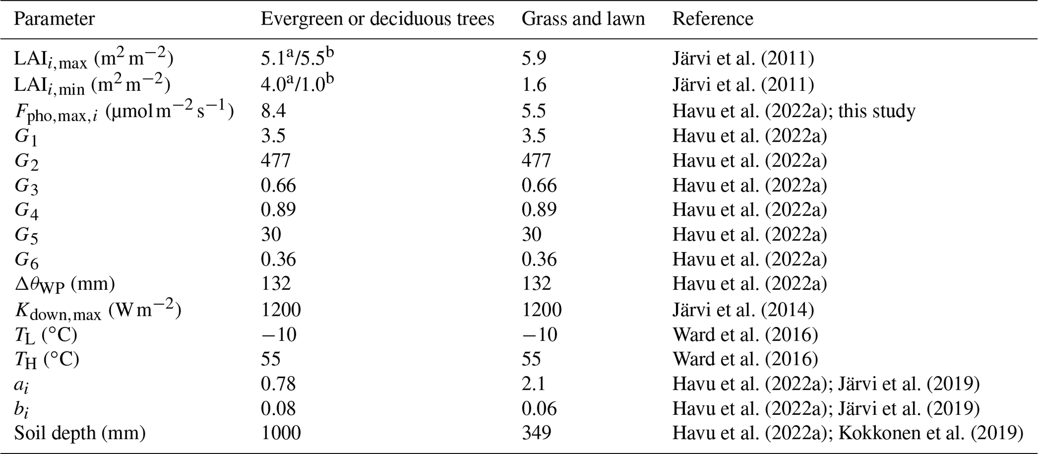
^a Evergreen tree. ^b Deciduous tree.

4.5.1 Sensitivity to vegetation-related parameters

In order to test the model's sensitivity of radiation and turbulent fluxes to vegetation-related parameters, four model cases are designed as follows.

1. The “Base” case. Control run where model parameters are considered “default” following Kokkonen et al. (2019) (Tables S2–S4). The exceptions are (1) parameters in the environmental response functions (Eqs. 4–7) of surface conductance that follow those by Havu et al. (2022a) (Table 2) because the product of response functions calculated following Kokkonen et al. (2019) is too low (95th percentile = 0.19) to obtain a realistic estimate of photosynthetic rate and (2) biogenic parameters for Eqs. (14) and (15) and soil properties that were updated following Havu et al. (2022a) (Table 2). In addition, F_pho,max for grass and lawn (5.5 $\mathrm{\mu }\mathrm{mol}{\mathrm{m}}^{-\mathrm{2}}{\mathrm{s}}^{-\mathrm{1}}$) is obtained from EC observations of CO₂ flux made over urban lawn in Helsinki in summer 2021 by fitting the conductance parameters ($F_{\text{pho},\text{max},\text{grass}}$, G₂–G₆) to the observations following Järvi et al. (2019) (Appendix D).

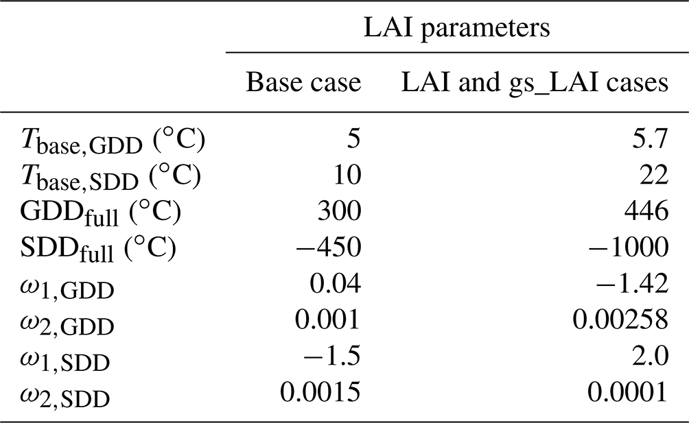
2. The “LAI” case. The same as the base case but the parameters for Eq. (1) describing the annual behavior of LAI are optimized using remotely sensed LAI and CMA-ES (Appendix A). The new optimized LAI parameters are compared with the base case in Table 3.

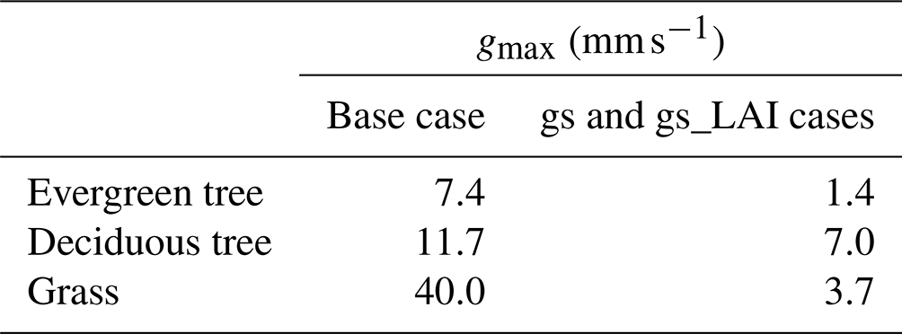
3. The “gs” case. The same as the base case but with g_max values collected from observational studies over vegetation species in Beijing (Appendix E). The site-specific g_max values are in general lower than the values used by the base case (Table 4).

4. The “gs_LAI” case. The same as the base case but with both LAI and g_max modified as described in the LAI and gs cases.

Table 3 Comparison in leaf area index (LAI) parameters between the base case and LAI and gs_LAI cases. All vegetation types (evergreen tree, deciduous tree, and grass) use the same LAI parameters within one case. The base case values are the same as in Järvi et al. (2011).

4.5.2 Sensitivity to radius of modeled area

SUEWS output will be evaluated against EC-measured turbulent fluxes, but the challenge is that the source area of the observations is different to the exact modeling domain. To consider the impact of the chosen modeling domain on model evaluation, we designed three additional model cases where circular areas around the IAP tower with different radii are considered. The default run is with the 1 km radius circle, but SUEWS is also run within 500, 750, and 1500 m circular areas, corresponding to the flux footprint of roughly 60 %, 70 %, and 80 %–90 %, respectively (Liu et al., 2012). Used vegetation parameters are as in the gs_LAI case, but land surface fractions, population, and traffic parameters are modified accordingly (Appendix F).

4.6 Statistical metrics for model evaluation

Common statistical metrics are used to quantify the model performance, including the coefficient of determination (R²), root-mean-square error (RMSE), and mean bias error (MBE). Simple linear regression is used to estimate the relationship between the model output and the observations, and the square of the correlation coefficient is taken as R². The other statistical metrics are defined as follows:

$$\begin{array}{}\text{(18)}& {\displaystyle }\mathrm{RMSE}=\sqrt{{\displaystyle \frac{{\sum }_{i=\mathrm{1}}^n(y_i-\widehat{y_i}{)}^{\mathrm{2}}}{n}}},\text{(19)}& {\displaystyle }\mathrm{MBE}={\displaystyle \frac{\mathrm{1}}{n}}\sum _{i=\mathrm{1}}^n(\widehat{y_i}-y_i),\end{array}$$

where $\widehat{y_i}$ is the modeled value and y_i the measured value. Statistical metrics are calculated at annual and seasonal scale, i.e., DJF (winter), MAM (spring), JJA (summer), and SON (autumn).

Table 4 Comparison of maximum conductances (g_max) between the base case and gs and gs_LAI cases. Parameters for the base case follow Järvi et al. (2011). More details can be found in Appendix E.

5 Results and discussion

5.1 Seasonal dynamics of the optimized LAI

The control base case simulates the onset of leaf growth and the ending of senescence reasonably well (Fig. 3). The performance of LAI modeling is further improved after the optimization (Appendix A). In the base case, the modeled LAI starts to increase rapidly from day-of-year (DOY) 70 and plateaus at DOY 105, which is too early when compared to the remotely sensed LAI (Landsat 7 LAI). The optimized LAI starts to grow at the same time but slightly slower and peaks 20 d later than in the base case. In autumn, LAI modeled by the base case drops rapidly at DOY 310, while the optimized LAI starts to decline rapidly at DOY 267. The LAI model with optimized parameters is better at capturing the behavior of senescence than in the base case.

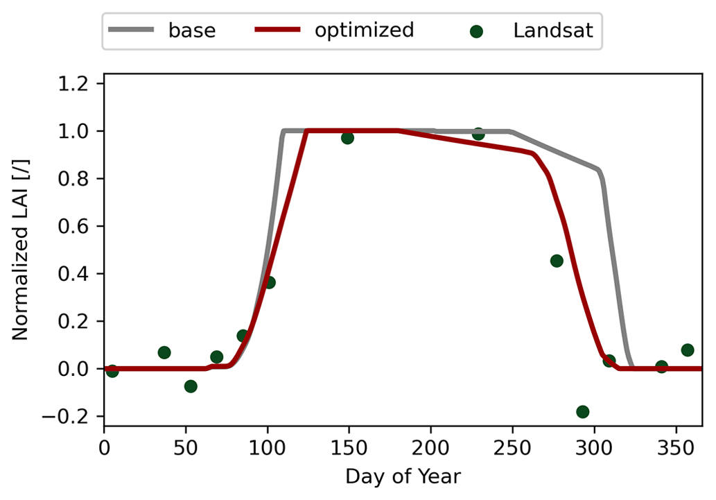
Figure 3 Normalized LAI in 2016, where the value 0 (1) represents the minimum (maximum) of LAI. “Base” denotes the modeled LAI for the base case, “Landsat” denotes the remotely sensed LAI of the adjacent park near the IAP tower, and “optimized” denotes the modeled LAI using the parameters derived with CMA-ES (Appendix A).

Although previous studies suggested that LAI was generally modeled well using default parameters following Järvi et al. (2011), Ward et al. (2016) reported that leaf growth is reached too early and suddenly in spring in two UK cities. In contrast, Ao et al. (2018) showed that the simulated LAI might be lower than reality when vegetation remained green in winter and spring in Shanghai, China. These lead to the bias in g_s and therefore Q_E estimates (Eqs. 2 and 3). In Beijing, the rainy season lasts from May to October, while the rest of the year is the dry season (Liu et al., 2012). It is possible that the distinct dry season leads to a lack of soil moisture in spring and autumn and thus influences the LAI seasonal dynamics if there is no external water input (Omidvar et al., 2022). However, the urban green spaces in Beijing are usually sufficiently or even excessively irrigated (Zhang et al., 2017). Observations also provided evidence to support the relationship between air temperature and phenological dynamics in the urban environment in Beijing (Lu et al., 2006; Luo et al., 2007). Therefore, the air temperature-dependent LAI model is applicable in Beijing, but the “default” LAI parameters might be not suitable. We recommend evaluating the LAI model when SUEWS is applied to a different city and deriving the optimal LAI parameters if necessary.

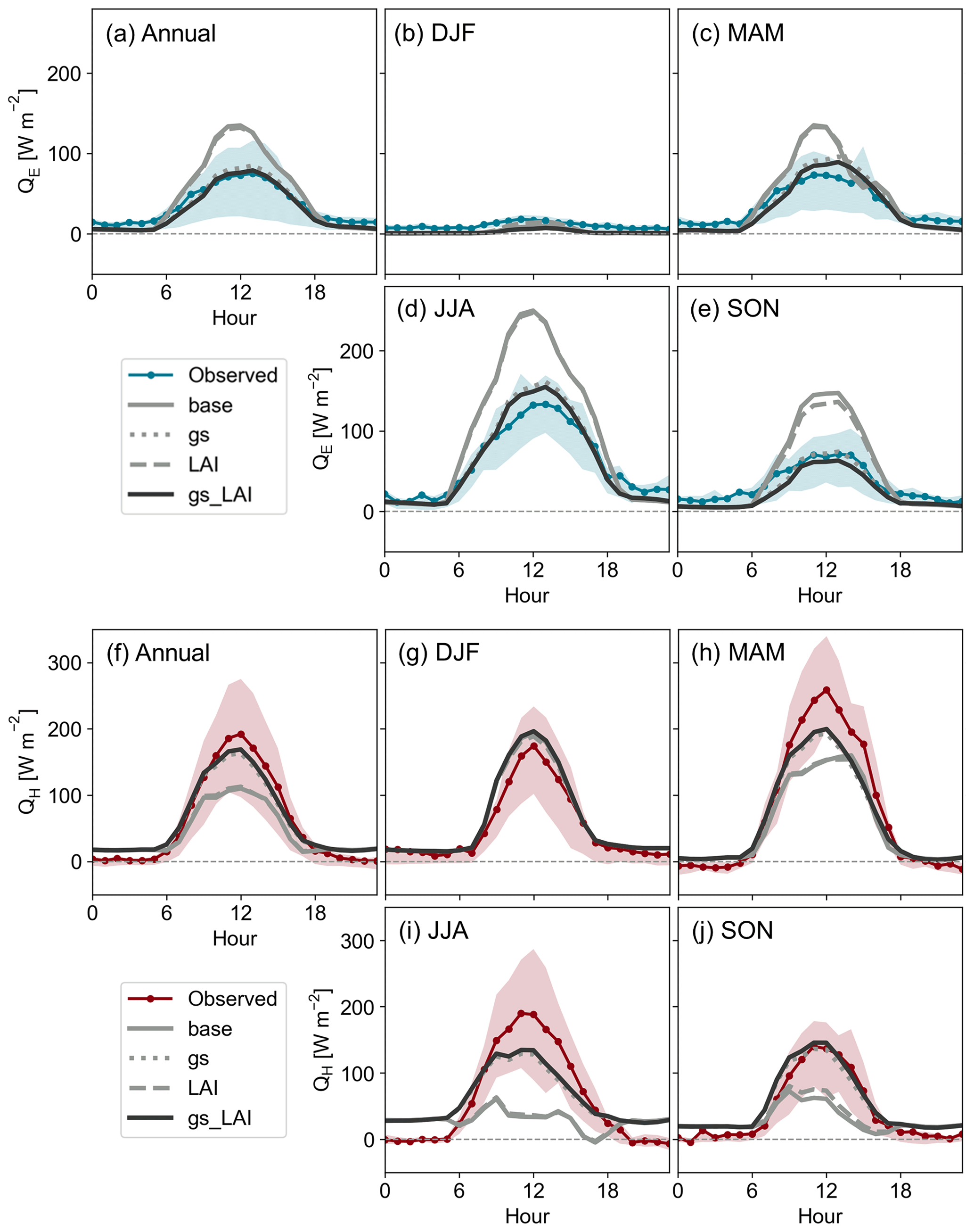
Figure 4 Annual and seasonal mean diurnal cycles of observed and modeled (a–e) latent heat flux (Q_E) and (f–j) sensible heat flux (Q_H) for the four model cases (base, gs, LAI, and gs_LAI) in the year 2016. The shaded area denotes the interquartile range.

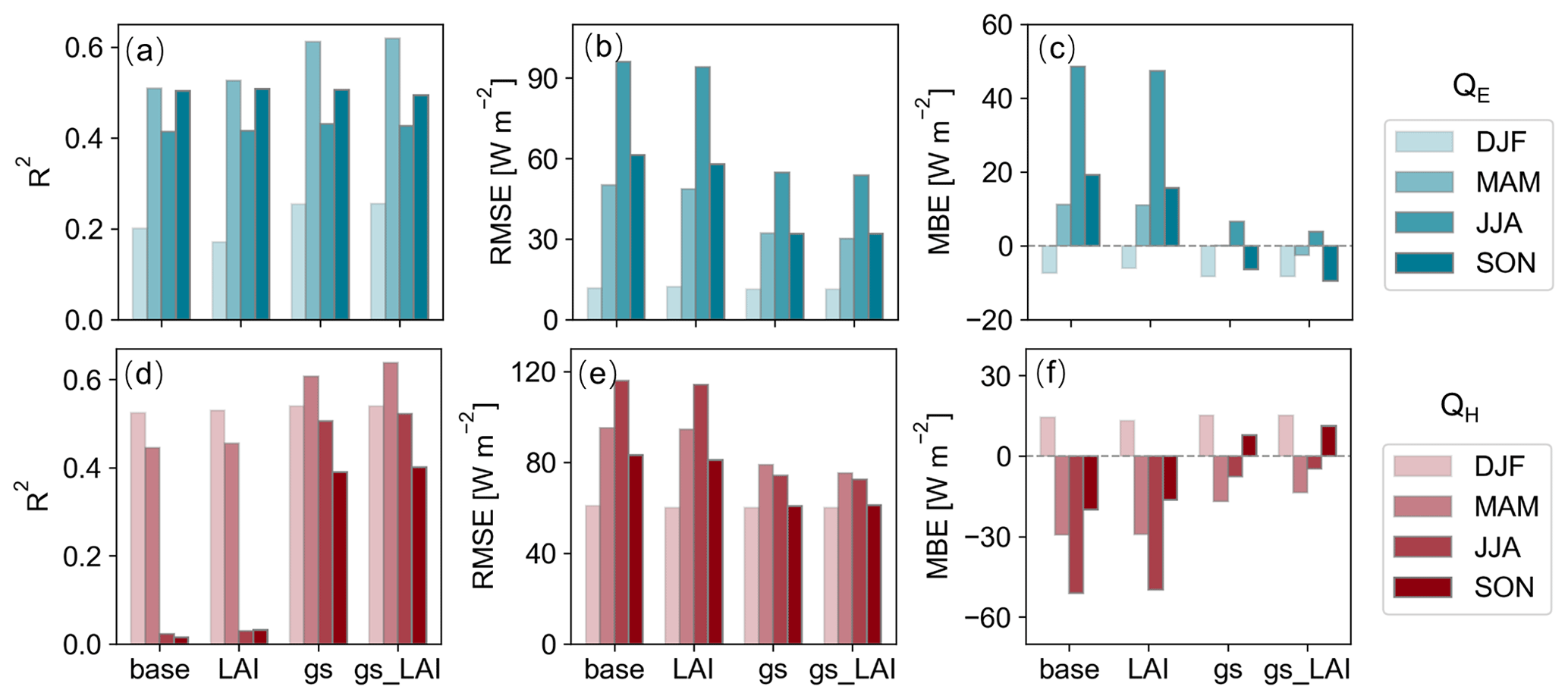
Figure 5 Model performance statistics R², RMSE, and MBE of (a–c) latent heat flux (Q_E) and (d–f) sensible heat flux (Q_H) for the four model cases (base, gs, LAI, and gs_LAI) in the year 2016.

5.2 Evaluation of turbulent heat flux modeling

Both observed Q_E and Q_H reach their maxima around noon (Fig. 4). The observed Q_E has the largest amplitude during the summer months, while Q_H during the spring months. All four model cases capture their diurnal cycles, but large differences in the amplitude and model performance are observed among the model cases (Fig. 5).

In the base case, the model overestimates Q_E (with MBE from −7.4 to 48.6 W m⁻²) except in winter months (Fig. 5). With the optimized LAI (the LAI case), model performance in Q_E remains virtually unchanged, with RMSE (12.1–94.1 W m⁻²) and R² (0.17–0.53) when compared to the base case (with RMSE 11.7–96.1 W m⁻² and R² 0.20–0.51) (Fig. 5a–c). Q_E is to a large extent determined by surface conductance, which is scaled by g_max of each vegetated surface for the modeled area (Eq. 3). Clear improvement is observed when the local g_max is used (the gs case), especially during summer. The overestimation of Q_E is largely reduced, RMSE drops to 11.3–54.7 W m⁻², and R² increases to 0.25–0.61. With both the optimized LAI and the local g_max introduced (the gs_LAI case), the R² is similar to the gs case, while RMSE slightly decreases by 1–2 W m⁻² in spring and summer compared to the gs case. Q_E is underestimated throughout the day in winter (MBE = −8.3 W m⁻²). Observational studies have shown that combustion-derived water vapor often contributes 5 %–10 % of total urban humidity during the heating season (Fiorella et al., 2018; Liu et al., 2022; Salmon et al., 2017). The observed Q_E ranges from 0 to 30 W m⁻² in winter when vegetation is dormant; this suggests that combustion and evaporation, as the dominant sources of Q_E, might lead to Q_E at this magnitude. The anthropogenic water vapor release might be underestimated by SUEWS in winter.

In SUEWS, Q_H is estimated as the residual of energy balance and is therefore directly affected by the modeled Q_E. As a result of overestimating Q_E in the base case, Q_H is greatly underestimated with MBE of −51.1–14.4 W m⁻² and RMSE of 60.9–116.0 W m⁻². R² values in summer months and autumn months are lower than 0.1. The model performance is barely improved by the optimized LAI (the LAI case) but it is noticeably improved after the local g_max is introduced (the gs case) (Fig. 5d–f). The best model performance for Q_H is obtained by the gs_LAI case, decreasing the magnitudes of MBE to −13.6–15.2 W m⁻² and RMSE to 60.1–75.3 W m⁻² and increasing R² to 0.40–0.64 (Fig. 5d–e).

Q_H is also influenced by Q_F. Nighttime Q_F in summer might be overestimated, leading to the overestimation in Q_H. Turbulent heat fluxes are also related to ΔQ_S. Both Q_E and Q_H correlate negatively with ΔQ_S (Eqs. 2 and 9). For instance, Q_E is underestimated, while Q_H is overestimated at noon in summer in the gs_LAI case. The decrease in ΔQ_S will lead to a simultaneous increase in Q_E and Q_H, lowering the bias of Q_H while increasing the bias of Q_E. Therefore, the adjustment of ΔQ_S can hardly improve the Q_E and Q_H modeling at the same time.

Our results suggest that the model performance of heat fluxes is more sensitive to the adjustment of g_max than to the change in LAI seasonal dynamics. By incorporating local LAI and g_max, SUEWS simulates the heat fluxes noticeably better, increasing R² by 0.03 (0.30) and decreasing RMSE by 27.0 (23.7) W m⁻² for Q_E (Q_H) compared to the base case.

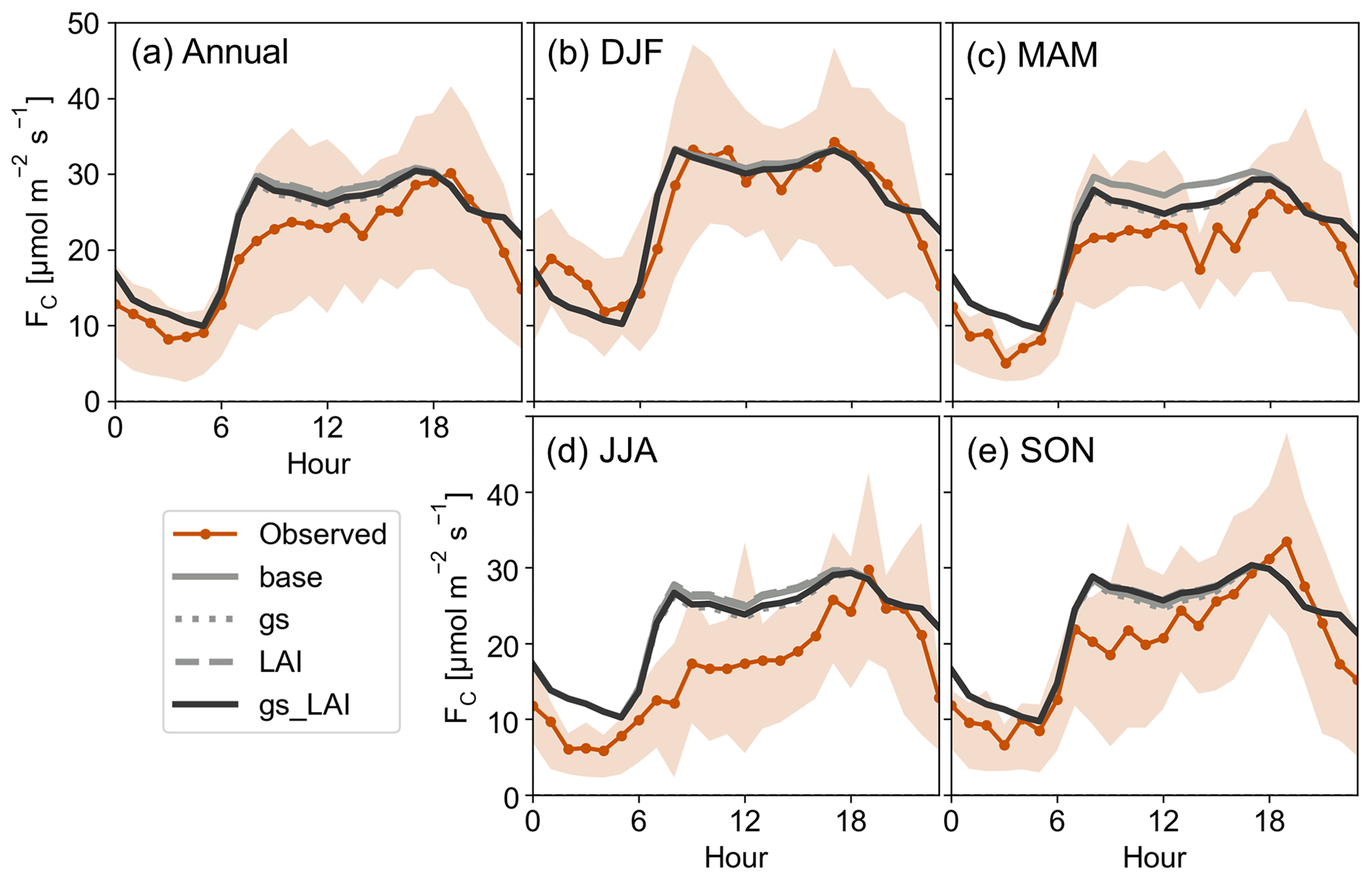
Figure 6 Annual and seasonal average diurnal cycles of observed and modeled CO₂ flux (F_C) for the four model cases (base, gs, LAI, and gs_LAI) in the year 2016. The shaded area denotes the interquartile range.

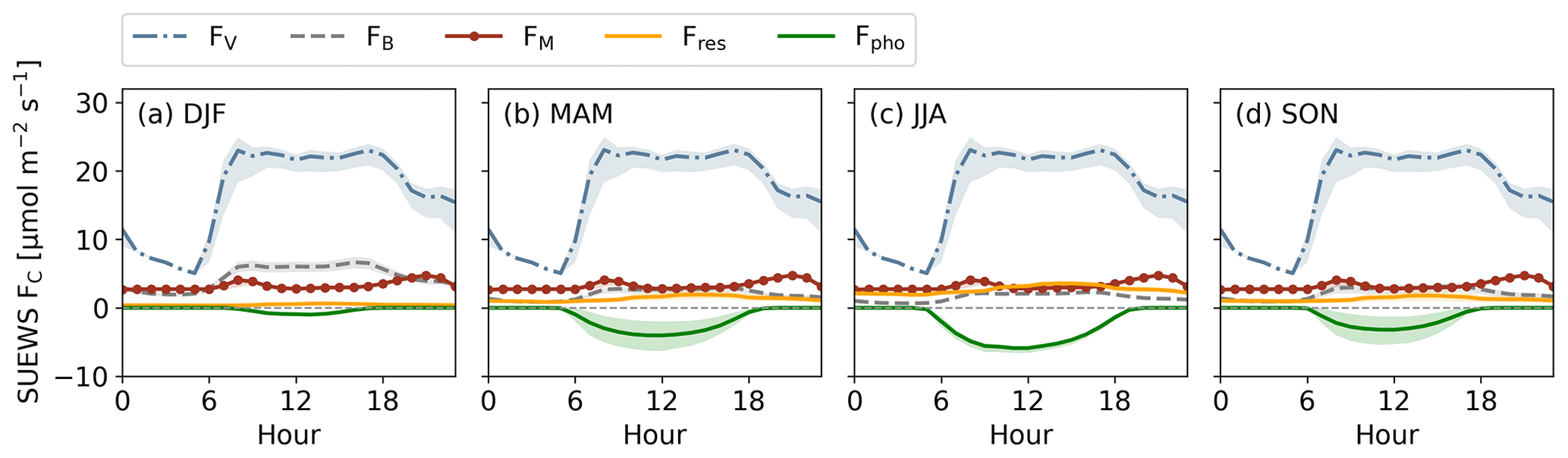
Figure 7 Seasonal average diurnal cycles of modeled CO₂ flux (F_C) components in the gs_LAI case in 2016. F_V denotes the CO₂ emissions from on-road traffic, F_B denotes buildings, F_M denotes human metabolism, F_res denotes vegetation and soil respiration, and F_pho denotes the CO₂ uptake by vegetation photosynthesis. Positive values indicate emissions of CO₂, and negative values indicate the uptake of CO₂ with respect to the atmosphere. The shaded area denotes the interquartile range.

5.3 Evaluation of CO₂ flux modeling

5.3.1 Model performance

SUEWS basically reproduces the average annual and seasonal diurnal cycle of observed F_C (Fig. 6). The diurnal behavior is dominated by on-road traffic emission, which reaches 22.6 and 23.0 $\mathrm{\mu }\mathrm{mol}{\mathrm{m}}^{-\mathrm{2}}{\mathrm{s}}^{-\mathrm{1}}$ for the morning peak and afternoon peak, respectively, during the rush hours (Fig. 7). Human metabolism (maximum 4.8 $\mathrm{\mu }\mathrm{mol}{\mathrm{m}}^{-\mathrm{2}}{\mathrm{s}}^{-\mathrm{1}}$) is the second largest source of CO₂ emissions. In winter, the building CO₂ emission has a maximum of 6.7 $\mathrm{\mu }\mathrm{mol}{\mathrm{m}}^{-\mathrm{2}}{\mathrm{s}}^{-\mathrm{1}}$ in the daytime. The maximum photosynthesis rate is 5.9 $\mathrm{\mu }\mathrm{mol}{\mathrm{m}}^{-\mathrm{2}}{\mathrm{s}}^{-\mathrm{1}}$ around noon in summer, while soil and vegetation respiration constantly serves as a CO₂ source with a rate lower than 3.6 $\mathrm{\mu }\mathrm{mol}{\mathrm{m}}^{-\mathrm{2}}{\mathrm{s}}^{-\mathrm{1}}$.

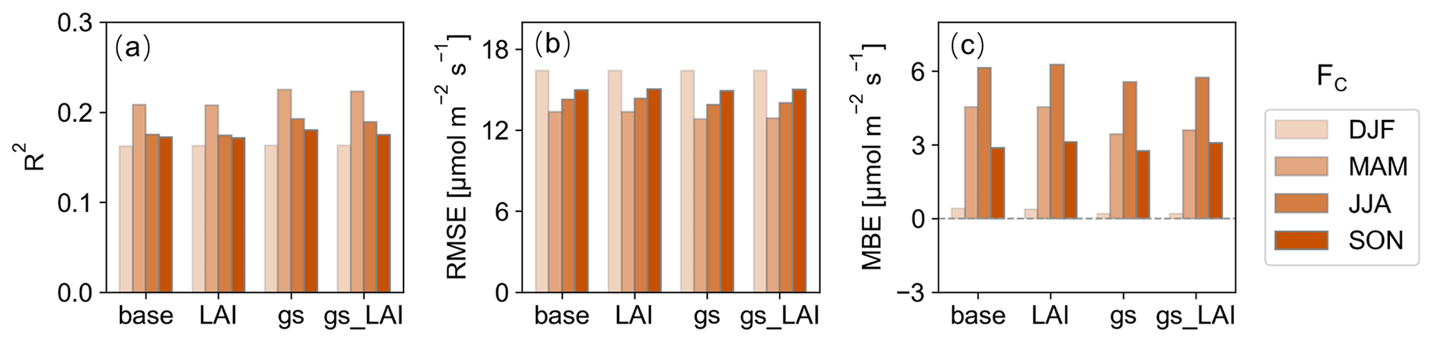
Figure 8 Model performance statistics for (a) R², (b) RMSE, and (c) MBE of CO₂ flux (F_C) for the four cases (base, gs, LAI, and gs_LAI) in the year 2016.

Each of the model performance statistics of F_C is of a similar magnitude among cases, indicating the F_C modeling is far less sensitive to the choices of g_max and LAI-related parameters than Q_E and Q_H shown in Sect. 5.2 (Fig. 8). Under the current parameterizations, F_res considers only air temperature (Eq. 15). The adjustments of g_max and LAI parameters affect the modeled heat fluxes, influencing 2 m air temperature, and finally F_res, but the difference in annual CO₂ release from respiration is less than 0.01 $\mathrm{kg}\mathrm{C}{\mathrm{m}}^{-\mathrm{2}}{\mathrm{yr}}^{-\mathrm{1}}$ among cases. F_pho is sensitive to the adjustments of g_max and LAI parameters. In the base case, the large values of g_max allow relatively high evapotranspiration (namely Q_E). As a result, the average Δθ during January and June is larger than 105 mm, which is only 27 mm lower than the wilting point deficit (Δθ_WP). The dry soil lowers the surface conductance and photosynthetic CO₂ uptake through the limiting function of g(Δθ) (Eq. 8). As the local g_max is introduced, the soil remains moister with Δθ lower than 75 mm throughout the year, allowing more favorable conditions for the photosynthetic CO₂ assimilation. The CO₂ assimilated through photosynthesis is 0.57 $\mathrm{kg}\mathrm{C}{\mathrm{m}}^{-\mathrm{2}}{\mathrm{yr}}^{-\mathrm{1}}$ in the gs case, which is 0.21 $\mathrm{kg}\mathrm{C}{\mathrm{m}}^{-\mathrm{2}}{\mathrm{yr}}^{-\mathrm{1}}$ higher than in the base case. The LAI reduction in spring and autumn in the gs_LAI case, on the other hand, directly limits surface conductance and photosynthesis (Eq. 14), leading to a decrease of 0.07 $\mathrm{kg}\mathrm{C}{\mathrm{m}}^{-\mathrm{2}}{\mathrm{yr}}^{-\mathrm{1}}$ in annual photosynthetic CO₂ uptake when compared to the gs case.

In SUEWS, photosynthetic and respiration rates are proportional to the fractions of vegetated surfaces, which account for only 29 % of the modeled area. The magnitude of F_pho is substantially lower than the traffic emission, making the effect of photosynthesis, as well as its response to the adjustments of g_max and LAI parameters, hardly visible in the F_C diurnal cycles (Fig. 6).

Expectedly, SUEWS has difficulty in capturing the hourly variability of F_C, resulting in the overall low R² (0.16–0.22) and high RMSE (12.9–16.4 $\mathrm{\mu }\mathrm{mol}{\mathrm{m}}^{-\mathrm{2}}{\mathrm{s}}^{-\mathrm{1}}$) (Fig. 8a). On the one hand, observed F_C has great variability at the hourly scale throughout the year, as indicated by the large interquartile range (Fig. 6). On the other hand, under the current parameterization, two of the anthropogenic F_C components are static: modeled traffic emission diurnal cycle is only dependent on whether it is a weekend or a weekday, and modeled human metabolism diurnal cycle is invariable throughout the year (Fig. 7), making it difficult to capture the extreme values. Other urban F_C bottom-up modeling studies also reported similar challenges in modeling F_C hourly variability in Helsinki and in Basel (Järvi et al., 2019; Stagakis et al., 2022).

SUEWS gives a reasonable estimate of annual accumulated F_C (8.6 $\mathrm{kg}\mathrm{C}{\mathrm{m}}^{-\mathrm{2}}{\mathrm{yr}}^{-\mathrm{1}}$), which is 15 % higher than the observed gap-filled value (7.5 $\mathrm{kg}\mathrm{C}{\mathrm{m}}^{-\mathrm{2}}{\mathrm{yr}}^{-\mathrm{1}}$). F_C is overestimated in all seasons, with the lowest MBE (0.2 $\mathrm{\mu }\mathrm{mol}{\mathrm{m}}^{-\mathrm{2}}{\mathrm{s}}^{-\mathrm{1}}$) in winter and the highest MBE (5.7 $\mathrm{\mu }\mathrm{mol}{\mathrm{m}}^{-\mathrm{2}}{\mathrm{s}}^{-\mathrm{1}}$) in summer (Fig. 8c).

There are multiple reasons to explain the difficulty in accurately capturing the diurnal cycle of the observed F_C for each season. First, the underlying seasonal variation in the diurnal wind pattern makes the F_C diurnal cycle from the NW quadrant more “seen” in winter and spring, while the diurnal cycle from the SE quadrant is more seen in summer and autumn (Fig. S2a–d). Second, the observed F_C varies noticeably with wind direction (Fig. S2e–h). An evident afternoon and evening F_C peak is observed from the NE and SE throughout the year. This might be attributed to the relatively high traffic volumes and more severe traffic congestion in the afternoon and evening than in the morning, especially at the nearby crossroads (Fig. 1d). The morning F_C peak only comes from the NE and NW and only during winter months, suggesting that there might be seasonal variation in the traffic pattern that is not captured by SUEWS. The noticeable increase in F_C in winter from the SE and NW indicates that the building heating emissions might mainly originate from these two sectors. However, SUEWS cannot consider this F_C's wind direction dependency as it simulates the overall flux from the simulation domain.

Apart from the wind direction, atmospheric stability influences the real-time footprint fetch of F_C (Crawford and Christen, 2015), but this is not considered in our study. Furthermore, there might be biases in simulating the seasonal cycles of F_C components. SUEWS might underestimate the vegetation photosynthetic rate or overestimate the CO₂ release from respiration due to the lack of site-specific biogenic parameters. Nonetheless, the model performance over the F_C diurnal cycle is reasonably good compared to a previous study (Järvi et al., 2019).

Uncertainties in traffic emission originate from the traffic rates and EFs. SUEWS adopts static traffic EFs and neglects the relationship between traffic emission and T_air as reported by Alvarez and Weilenmann (2012) and Fontaras et al. (2017). In order to examine the impact of seasonal variation of T_air in traffic emission, correction is conducted using the regression function following Zhang et al. (2021), but only a marginal difference is seen at monthly scale: a difference of 3 % in winter, −2 % in spring, ∼ 0 % in summer, and −1 % in autumn. Therefore, we believe that the static traffic EFs adopted by SUEWS can provide reasonable traffic emission values without considering the seasonal dynamics of T_air.

Järvi et al. (2019) reported that using a different coefficient of CO₂ release per capita (C_M) led to a 6 % decrease in the human metabolic CO₂ emission estimate. If C_M is set to a daily mean value of 242 $\mathrm{\mu }\mathrm{mol}{\mathrm{m}}^{-\mathrm{2}}{\mathrm{s}}^{-\mathrm{1}}$ (Prairie and Duarte, 2007) instead of the current values (Table 1), the human metabolic emission will increase and the annual F_C will be 4 % higher than the original estimate.

Building emissions are calculated based on the Q_F estimates and heating fraction. Modeled average Q_F in December is 52.7 W m⁻², which is higher than another model estimate (21.6 W m⁻²) in the modeled area (Wang et al., 2020). Observations of Q_F are rarely available, and thus these Q_F estimates have not yet been validated. The representativeness of the heating fraction estimated from yearbook statistics is yet to be examined because the location and heating capacity of heating boilers within the modeled area is unknown. However, the building emission estimate (0.97 $\mathrm{kg}\mathrm{C}{\mathrm{m}}^{-\mathrm{2}}{\mathrm{yr}}^{-\mathrm{1}}$) falls in the range of estimates (∼ 0–3.0 $\mathrm{kg}\mathrm{C}{\mathrm{m}}^{-\mathrm{2}}{\mathrm{yr}}^{-\mathrm{1}}$) by other cities (Björkegren and Grimmond, 2018; Christen et al., 2011; Järvi et al., 2019; Moriwaki and Kanda, 2004).

The modeled CO₂ release by respiration is larger than CO₂ assimilated through photosynthesis in our study. At the annual scale, urban vegetative surfaces can have a net CO₂ uptake (Awal et al., 2010; Konopka et al., 2021) but may also have a net emission (Peters and McFadden, 2012). Admittedly, bias might exist in biogenic CO₂ flux estimates since the parameters used in this study are derived from the observations over street trees in Helsinki and over a lawn at Ossinlampi, Finland, where the climate and vegetative species are different from Beijing. With these parameters, the model might underestimate the CO₂ sequestrated by the local vegetation or overestimate the CO₂ release by respiration.

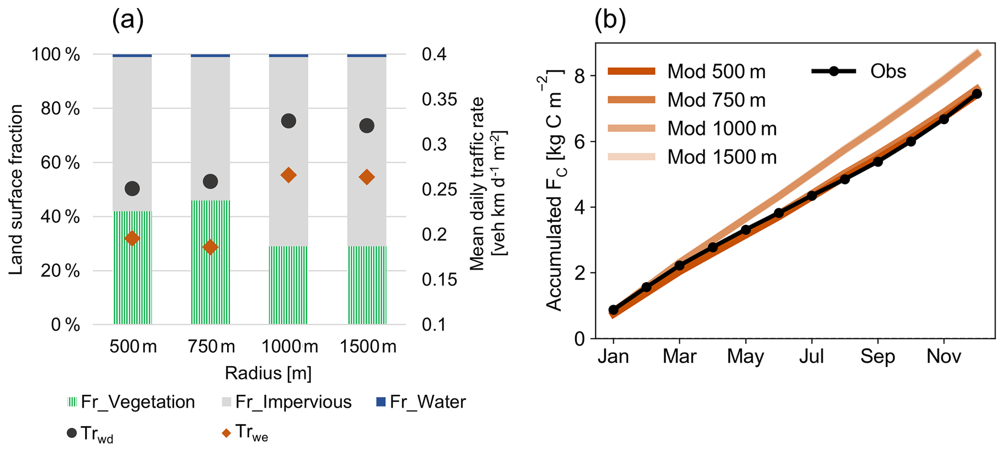
Figure 9 (a) Land use fraction and mean daily traffic rate (Tr_wd/we) and (b) accumulated CO₂ flux (F_C) for the modeling domain, with the radius ranging from 500 m to 1500 m. “Wd” denotes weekday, “we” denotes weekend, “Mod” denotes modeled F_C, and “Obs” denotes observed F_C. Note that in (b) the lines for Mod 500 m and Mod 750 m nearly overlap, while the lines for Mod 1000 m and Mod 1500 m nearly overlap.

5.3.2 The impact of the modeling domain size

The surroundings of the IAP tower are heterogeneous in terms of land surface fraction and mean daily traffic rate (Fig. 9a). The fraction of vegetated surfaces is higher closer to the tower than further away due to the green spaces adjoining the IAP tower (Fig. 1b). Additionally, there is a traffic hot spot on the 3rd Ring North Road located 850 m to the south of IAP tower (Fig. 1d), where the traffic rate is 2 to 7 times the value for the other roads inside the circle of a 1000 m radius (figure not shown). A large increase of 26 % in daily traffic rate is seen when the radius of modeling domain is 1000 or 1500 m when compared to domains with lower radii (Fig. 9a). Thus, the modeled annual accumulated F_C largely depends on the modeling domain size chosen, giving estimates of 7.4, 7.6, 8.6 ,and 8.7 $\mathrm{kg}\mathrm{C}{\mathrm{m}}^{-\mathrm{2}}{\mathrm{yr}}^{-\mathrm{1}}$ for the radii of 500, 750, 1000, and 1500 m, respectively. Observational annual F_C (7.5 $\mathrm{kg}\mathrm{C}{\mathrm{m}}^{-\mathrm{2}}{\mathrm{yr}}^{-\mathrm{1}}$) falls within this range, which indicates the good model performance of SUEWS (Fig. 9b).

The turbulent flux modeling is usually evaluated over a fixed extent, such as a circle with a certain radius, to approximate the flux source area (Demuzere et al., 2017; Järvi et al., 2019). However, when a circle with the radius ≥ 1000 m is selected to approximate the ≥ 80 % footprint fetch in our study, SUEWS does not give the closest estimate of annual F_C. This can be explained by the mismatch between the modeling domain and the real flux source area – the single fixed-extent modeled area cannot perfectly represent the land surface characteristics (e.g., the nonuniform land cover and human activities), biassing turbulent flux modeling (Chu et al., 2021; Laine et al., 2009). First, the accumulated footprint area of the observed fluxes is irregular in shape and varies with time (Liu et al., 2012). Second, the relative contribution to flux from the land surface decreases as the distance to the measurement instrument increases (Christen et al., 2011; Rebmann et al., 2005). Thus, when the modeling domain is a 1000 m radius circle, the model might underestimate the relative contribution from the adjacent vegetated surface and overestimate the contribution of the traffic hot spot at the edge of 80 % footprint fetch.

Regardless of the modeling domain size, traffic is the dominant CO₂ source, contributing 59 %–70 % to the total CO₂ emissions, followed by human metabolism (14 %–18 %), building energy use (11 %–14 %), and CO₂ release by vegetation and soil respiration (6 %–10 %). Vegetation photosynthesis offsets only 5 %–10 % of the total annual CO₂ emissions (Fig. 10). Several bottom-up modeling studies show that the on-road traffic is the greatest source in a densely built neighborhood, contributing to 70 % in central London, 61 % in Helsinki, 53 %–78 % in Tokyo, and 70 % in Vancouver, while human metabolism also plays an important role, contributing 5 %–39 % to the annual total F_C (Björkegren and Grimmond, 2018; Christen et al., 2011; Järvi et al., 2019; Moriwaki and Kanda, 2004). Our results are in general agreement with these studies. The contribution of the local building emissions within the study area is more variable among cities: a contribution of 70 % is reported in Basel (Stagakis et al., 2022), while ∼ 0 % is reported in Helsinki (Järvi et al., 2019), and our estimate falls in this range. The direct CO₂ sequestration by urban plants is minor compared with the total CO₂ emissions in this densely built neighborhood, which is in general agreement with Pataki et al. (2011) and Christen et al. (2011). For more accurate biogenic component estimates in Beijing, photosynthetic and respiration observations over local species are needed in the future.

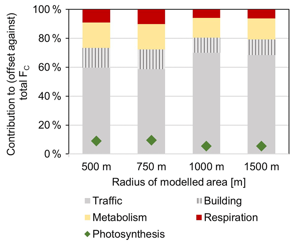
Figure 10 The contribution to total CO₂ emissions by each component at the annual scale for the modeled area with a radius ranging from 500 to 1500 m. Note that for photosynthesis the percentages denote the offset against total CO₂ emissions.

6 Conclusions

A correct description of vegetation is vital in order to simulate the energy and CO₂ fluxes over urban surfaces using the urban land surface model SUEWS. In this study, the impact of selecting appropriate vegetation parameters, including LAI parameters and g_max, on simulating the surface fluxes is examined in Beijing, China. In addition, the newly developed CO₂ emissions module in SUEWS is evaluated against EC measurements.

The model performance of heat fluxes (Q_E and Q_H) is more sensitive to the adjustment of g_max than to the change in LAI seasonal dynamics in our study area. The LAI model has been improved by using CMA-ES to optimize the LAI parameters with a remotely sensed LAI product, providing more realistic vegetation phenological dynamics, especially for the senescence season. The parameter g_max was parameterized according to leaf-level observations of vegetation species in Beijing. By incorporating local LAI and g_max, SUEWS simulates the heat fluxes noticeably better, increasing R² by 0.03 (0.30) and decreasing RMSE by 27.0 (23.7) W m⁻² for Q_E (Q_H), and showing more realistic seasonal dynamics when compared to EC observations.

F_C modeling appears to be less sensitive to the choice of LAI-related parameters and g_max. Only one of the F_C components, F_pho, responds noticeably to them. SUEWS can catch the general diurnal and seasonal behavior of F_C but tends to overestimate F_C, especially in summer months. We also tested the influence of chosen modeling domain size on simulated F_C. By selecting the modeled radii of circular areas ranging from 500 to 1500 m (i.e., an accumulated footprint area from 60 % to 80 %–90 %), the modeled annual F_C ranges from 7.4 to 8.7 $\mathrm{kg}\mathrm{C}{\mathrm{m}}^{-\mathrm{2}}{\mathrm{yr}}^{-\mathrm{1}}$, which is comparable with the EC observations (7.5 $\mathrm{kg}\mathrm{C}{\mathrm{m}}^{-\mathrm{2}}{\mathrm{yr}}^{-\mathrm{1}}$). This shows that the model also performs well on the annual scale. Regardless of the modeling domain size, traffic is the dominant CO₂ source, contributing 59 %–70 % to the total CO₂ emissions, followed by human metabolism (14 %–18 %), buildings (11 %–14 %), and CO₂ release by vegetation and soil respiration (6 %–10 %). Vegetation photosynthesis offsets only 5 %–10 % of the CO₂ emissions.

We highlight the importance of choosing more site-specific LAI parameters or g_max when SUEWS is used for heat flux modeling before the more advanced application such as urban climate and hydrological modeling. Observations are needed to support more accurate parameterizations of biogenic CO₂ fluxes. We believe that the bottom-up approach to model F_C by SUEWS can be a promising tool in capturing the CO₂ emission hot spots, quantifying the relative contribution of the local CO₂ sources, and assisting us in mitigating urban CO₂ emissions.

Appendix A: Workflow of LAI parameters optimization

In SUEWS, LAI influences the surface conductance and subsequently Q_E and F_pho (Sect. 2). A workflow for parameter derivation for the LAI sub-model based on remotely sensed data is designed for natural ecosystems (Omidvar et al., 2022). However, vegetation in urban areas behaves differently from natural ecosystems (Zhang et al., 2022) and needs to be considered separately. Therefore, we propose a workflow to obtain the parameters for urban area based on remotely sensed LAI and covariance matrix adaptation evolution strategy (CMA-ES). This workflow can also be applied to natural ecosystems. The related data and codes are openly available (Zheng et al., 2022).

Covariance matric adaptation evolution strategy (CMA-ES) is one of the strategies for numerical optimization of non-convex problems. It is based on the principle of biological evolution. The evolution strategy takes a certain number of individuals (candidate solutions) in a stochastic way, selects individuals based on the fitness, and repeats this process for generations so that a better or an optimal solution is obtained. Adaptation of the covariance matrix amounts to learning a second-order model of the underlying objective function. Compared with classic optimization methods, CMA-ES requires neither derivatives nor an objective function; it only requires the ranking of candidate solutions. Besides, CMA-ES outranks many of other optimization algorithms, performing especially strongly for “difficult functions” or larger dimensional search spaces (Hansen et al., 2010).

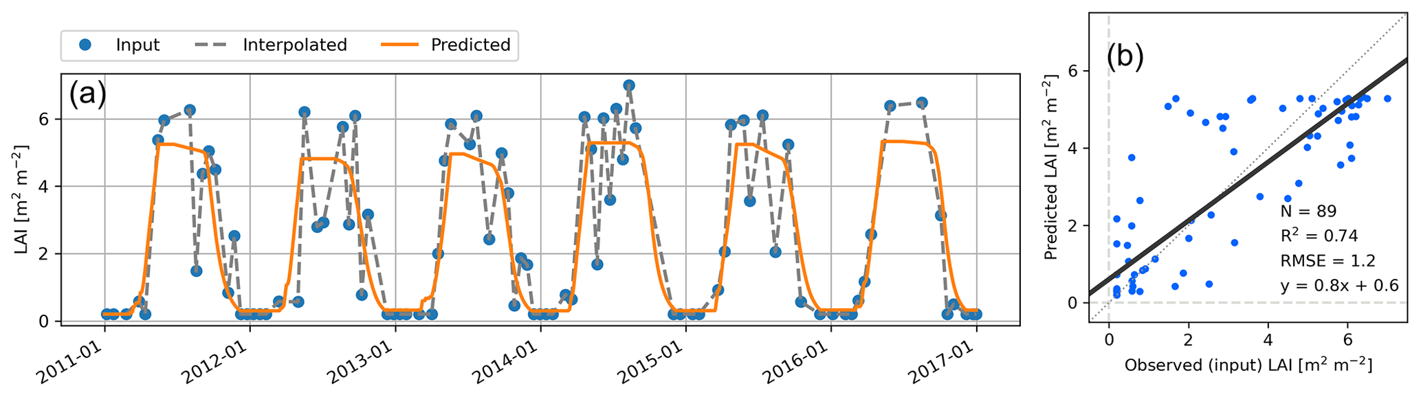
Figure A1 (a) Time series of the input LAI, the interpolated LAI, and the predicted LAI and a (b) comparison of the predicted LAI against the observed LAI.

Taking our study area as an example, the LAI parameters are optimized as follows:

1. LAI derivation. A 6-year time series (2011–2016) of LAI of the vegetation in a park near the IAP tower is calculated from the atmospherically corrected surface reflectance provided by USGS Landsat 7 Enhanced Thematic Mapper + (ETM+) (30 m spatial resolution) via the Google Earth Engine Data Catalog (Masek et al., 2006). The time series is treated as the “original LAI”.

2. Spikes removal. There are outliers in the LAI time series caused by instrument problems, uncertainties in the retrieval algorithm, and cloud contamination. Values larger than 10 m² m⁻² and negative values are first removed. The LAI values during December and January are set to a fixed value, i.e., the average of these months (0.2 m² m⁻²), in order to reduce the noise in winter and improve the optimization performance.

3. Scaling the original LAI to the canopy level. The original LAI might be noticeably lower than the measured LAI at the canopy level over a homogeneous vegetated surface. Nonetheless, the original LAI provides the signals of vegetation phenology (e.g., leaf out, peak growing season, leaf fall). In order to give a more realistic estimate of LAI at the canopy level, the original LAI needs to be scaled. Therefore, LAI_max and LAI_min need to be given manually, preferably based on observational studies over local species. Here, the original LAI is scaled to allow the optimized LAI to reach 5–6 m² m⁻² in the peak growing season as reported by an observational study in Beijing (Wang et al., 2021). The canopy-level LAI is marked as the “input LAI” for the process of optimization and marked as the “observed LAI” for the process of evaluation.

4. Interpolation. The observed LAI values are linearly interpolated between values to obtain a daily time series, marked as the “interpolated LAI”.

5. Parameter derivation using CMA-ES. The time series of interpolated LAI and T_air are subjected to CMA-ES to optimize the parameters. Using the LAI model and the derived parameters, LAI is calculated and marked as the “predicted LAI”.

Despite the spike removal step, noise is observed in the LAI time series such as the abrupt drop and recovery during summer. Smoothing techniques are used to extract valid information from the satellite data with noise. In other words, the overall pattern (e.g., the moving average) of the time series is the information of interest, and CMA-ES has successfully reproduced the overall pattern out of the input LAI time series contaminated by noise (Fig. A1a). Moreover, the LAI has been “scaled” as shown in the scaling step to allow the output LAI to reach 5–6 m² m⁻² in order to avoid the underestimation of the predicted values. Therefore, the noise in the input LAI during summer is kept since it has little impact on the outcome. We conclude that the model performance is overall good (with R² = 0.74 and RMSE = 1.2 m² m⁻²) (Fig. A1b).

Appendix B: Evaluation of WFDE5 reanalysis against observed meteorological variables

To force SUEWS, local-scale meteorological data within the inertial sublayer is required. However, they can be unavailable for the area and period desired. Reanalyses provide spatially and temporally complete datasets, which might make the modeling run easier for users. Kokkonen et al. (2018) and Kokkonen et al. (2019) evaluated one of the reanalyses, WATCH Forcing Data ERA-Interim (WFDEI), suggesting that WFDEI can serve as the forcing of SUEWS but should be corrected beforehand when the bias is large.

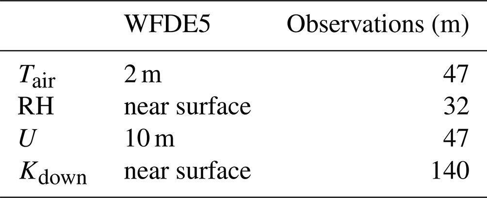
WFDE5 is a bias-corrected dataset of near-surface meteorological variables derived from the fifth generation of the European Centre for Medium-Range Weather Forecasts (ECMWF) atmospheric reanalysis (ERA5) (Cucchi et al., 2021). It is generated using the same methodology as WFDEI, and provides a single layer at 0.5^∘ spatial resolution and hourly temporal resolution. The evaluation of WFDE5 and the use of it as forcing data to SUEWS have been neglected so far. Here, we compare WFDE5 against observed meteorological variables including air temperature (T_air), relative humidity (RH), wind velocity (U) at 47 m, and incoming shortwave radiation (K_down) at 140 m on the IAP tower (Liu et al., 2012). The evaluation of K_down is conducted from May 2010 to June 2011, and the rest is conducted from January 2010 to December 2011. All the observed variables are resampled from 30 min to 1 h resolution.

With the difference in height for each meteorological variable (Table B1), however, WFDE5 is close to the observed data as a whole (Fig. B1). Compared with the observed data, WFDE5 T_air is lower, RH is higher, U is lower, and K_down is higher. WFDE5 may underestimate T_air and overestimate RH due to it neglecting the urban anthropogenic heat release; WFDE5 might overestimate K_down due to insufficient consideration of aerosol's effect in decreasing solar radiation received by the urban surface. The lower U of WFDE5 can be explained by the lower height compared with the observations (Table B1). If the WFDE5 U is adopted as a forcing of SUEWS, aerodynamic resistance might be overestimated, and therefore Q_E might be underestimated.

Table B1 The height of WFDE5 and observed meteorological variables.

Admittedly, some meteorological variables of WFDE5 correlate poorly with the observations in a particular season (e.g., R² = 0.13 for U in JJA). However, the overall high R² and low RMSE and MBE in magnitude suggest that WFDE5 provides reasonably good estimates of each meteorological variable (Table B2). Therefore, WFDE5 is adopted as the forcing data of SUEWS in this study.

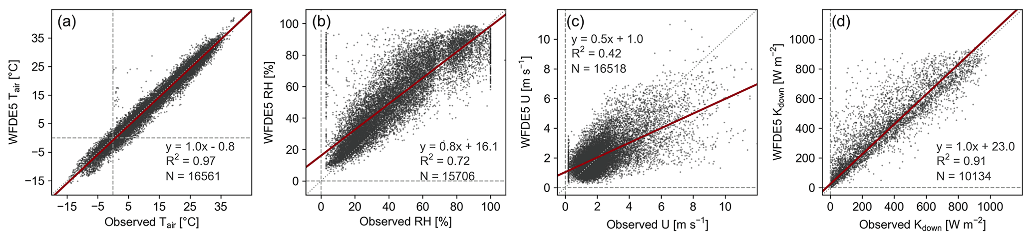
Figure B1 Comparison of WFDE5 and observed meteorological variables including (a) air temperature (T_air), (b) relative humidity (RH), (c) wind velocity (U), and (d) incoming solar radiation (K_down) at an hourly resolution.

Table B2 Statistics for WFDE5 compared against the observed meteorological variables.

Appendix C: Evaluation of radiation fluxes

The radiation parameterization scheme Net All-wave Radiation Parameterization (NARP) does not involve g_max or LAI. As expected, the four experiments (Sect. 4.5.1) give identical radiation flux components in the output. Therefore, only the gs_LAI case is further analyzed here.

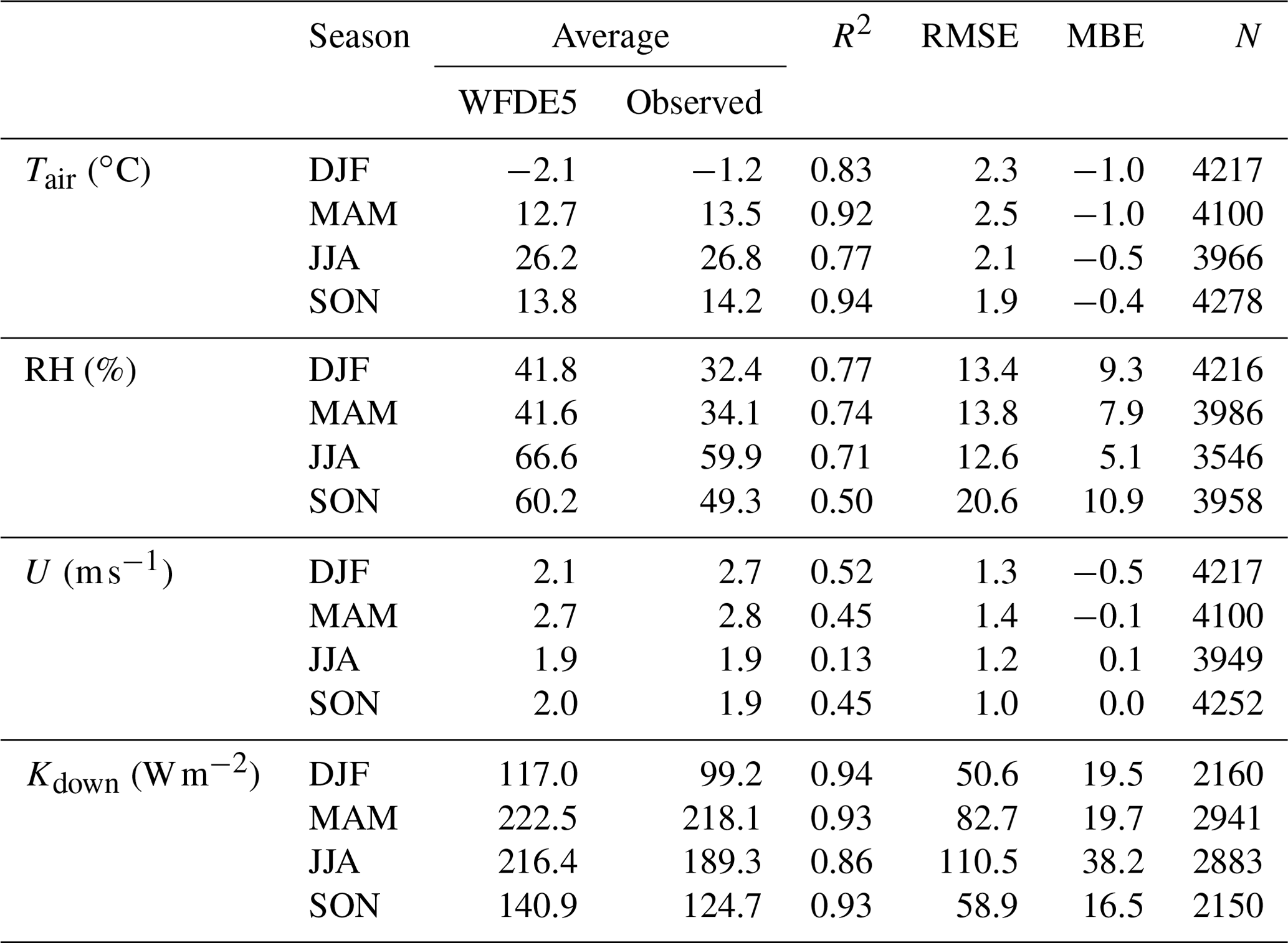
The model performance of SUEWS in simulating radiation fluxes is good (Fig. C1, Table C1), and it can reproduce the diurnal cycle of each radiation flux well (Fig. C2). K_up is overestimated in all seasons, with MBE ranging from 0 to 10 W m⁻². This overestimation can at least partly be explained by the positive bias (MBE > 15 W m⁻² in all seasons) of WFDE5 K_down when compared to the observed K_down (Appendix B). The overestimation in K_up can also be caused by surface albedo. Observational studies have shown that the urban surface albedo near the IAP tower varies between 0.1 and 0.15 with season (Jiang et al., 2007; Miao et al., 2012). The annual bulk albedo for the modeling domain given to SUEWS is 0.14, which is relatively high but still consistent with the observations. A larger positive bias in K_up is observed in summer than in winter. Surface albedo is influenced by many factors, such as surface wetness and street canyon trapping effect (Ao et al., 2016; Dou et al., 2019), which have not yet been considered by SUEWS. By simply (1) adjusting the albedos for surface types following Ward et al. (2016) and (2) allowing albedo for vegetation to vary from a lower value in summer to a higher value in winter (Table S5), the RMSE for K_up decreases for all seasons, especially in summer (from 18.0 to 13.6 W m⁻²), but this only has a minor impact on Q_N modeling (Table S6).

Table C1 SUEWS model performance statistics for radiation fluxes. The abbreviations are the same as those in Fig. C1. Note that K_down is an input of SUEWS, while the others are outputs of SUEWS.

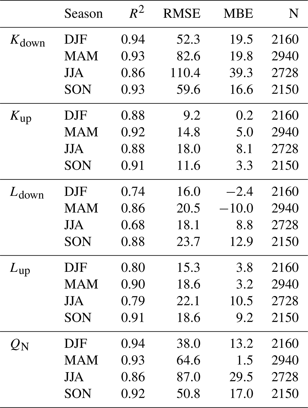
The average seasonal and diurnal cycles of L_down are well captured by the model (Fig. C2i–l), although R² (0.68–0.88) is lower than with other radiation fluxes. The difference might result from the discrepancy between the observed and modeled cloud fraction as clear skies and overcast conditions are especially difficult to capture using the radiation model NARP, as also reported by Ao et al. (2016) and Ward et al. (2016). The diurnal amplitude of L_up is slightly overestimated by SUEWS (Fig. C2m–p). The model tends to overestimate L_up, particularly at high values of L_up (Fig. C1m–p). The values of emissivity of building materials used in SUEWS might be slightly higher than in reality. L_up is also dependent on K_down in NARP. Therefore, the overestimation of L_up can partly be explained by the overestimated K_down provided by WFDE5, especially around noon and in summer.

We conclude that SUEWS is applicable to provide a realistic estimate of radiation fluxes in Beijing, in general accordance with previous studies (Järvi et al., 2014; Karsisto et al., 2016; Ward et al., 2016), despite the absence of site-specific parameters.

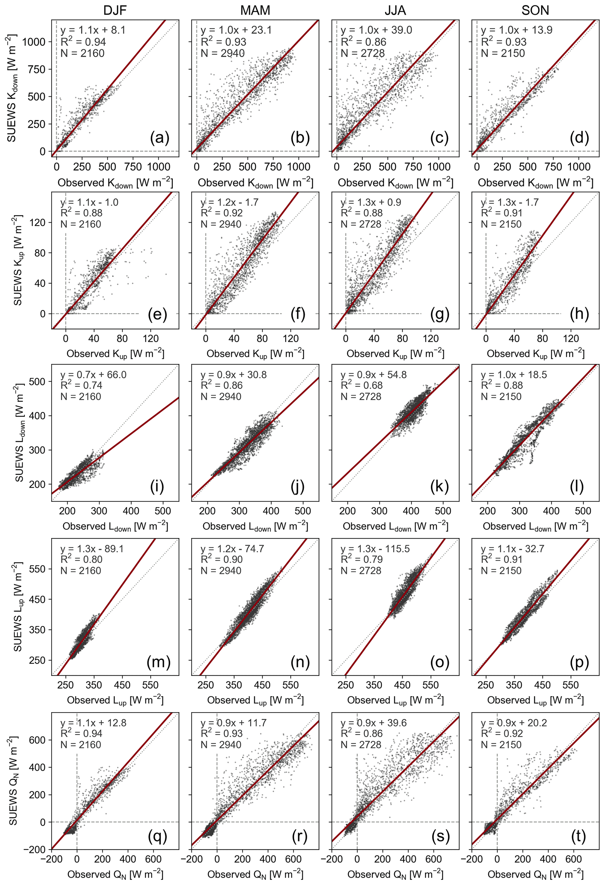
Figure C1 Input or modeled vs. observed hourly radiation fluxes, including (a–d) incoming solar radiation (K_down), (e–h) outgoing shortwave radiation (K_up), (i–l) incoming longwave radiation (L_up), (m–p) outgoing longwave radiation (L_up), and (q–t) net radiation (Q_N) from May 2010 to June 2011. Note that while K_down is input, the rest are model output.

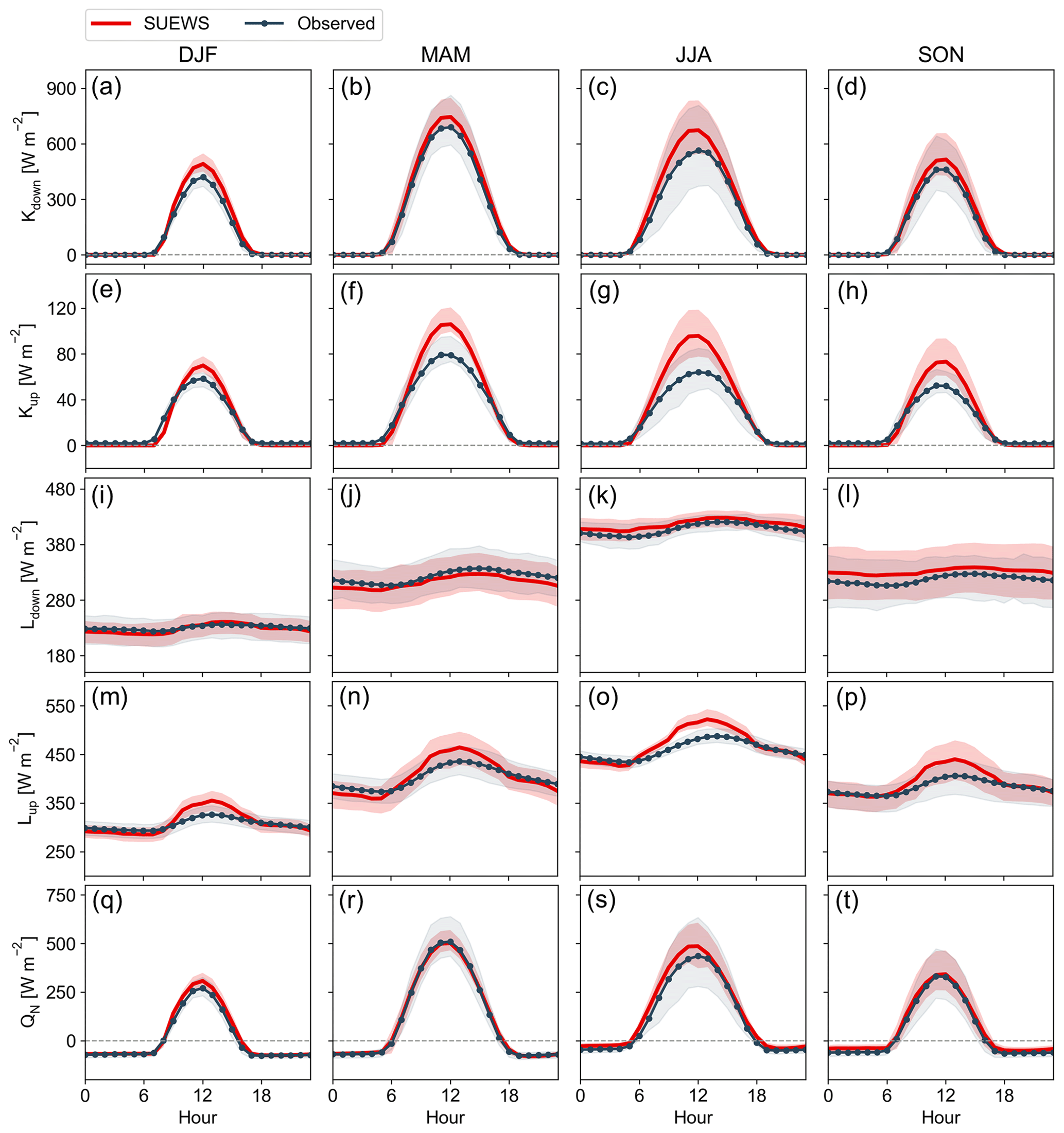
Figure C2 Average diurnal cycle of input or modeled and observed hourly radiation fluxes by season, including (a–d) incoming solar radiation (K_down), (e–h) outgoing shortwave radiation (K_up), (i–l) incoming longwave radiation (L_up), (m–p) outgoing longwave radiation (L_up), and (q–t) net radiation (Q_N) from May 2010 to June 2011. The shaded area denotes the standard deviation. Note that while K_down is input, the rest are model output.

Appendix D: Fitting the maximum photosynthetic rate for the grass and lawn vegetation type

In order to find the maximum photosynthetic rate for the vegetation type of grass to be used in SUEWS simulation, the environmental response functions g(T_air), g(Δq), g(Δθ), and g(K_down) in Eq. (14) were fitted to observations from an eddy covariance (EC) station (60^∘11^′16.02^′′ N, 24^∘49^′56.85^′′ E) situated on an urban lawn in Espoo, Finland. A 1.2 m high EC tower was located at the center of the urban lawn covering an area of 0.7 ha. The EC setup consisted of a three-dimensional sonic anemometer (Metek GmbH, Germany) for measuring the three wind components and sonic temperature and a closed-path infrared gas analyzer (LI-7200; LI-COR, Lincoln, NE, USA) for measuring the CO₂ and H₂O mixing ratios. The gas analyzer inlet was positioned 13 cm below the anemometer, and air was drawn into the gas analyzer using a 60 cm length of steel tube, having an inner diameter of 4.57 mm and a mean flow rate of 12 L min⁻¹. The tube was heated to avoid water vapor condensation on tube walls. The raw EC data were sampled at 10 Hz and stored for post-processing. The steps before 30 min flux calculations consisted of despiking, linear detrending, and planar fitting of the raw data.

The biogenic CO₂ flux F_C,bio from EC measurements was partitioned into F_res and F_pho using the nighttime temperature dependency of F_res. The nighttime F_C,bio was considered nighttime F_res, and it was related to the observed T_air by fitting the exponential model:

$$\begin{array}{}\text{(D1)}& F_{\text{res}}=a_{\text{grass}}\cdot \text{exp}\left(T_{\text{air}}{b}_{\text{grass}}\right),\end{array}$$

where a_grass and b_grass are parameters controlling the temperature dependency. The nighttime temperature dependency of F_res was then extrapolated to daytime, and F_pho was then calculated by

$$\begin{array}{}\text{(D2)}& F_{\text{pho}}=F_{\mathrm{C},\text{bio}}-F_{\text{res}}.\end{array}$$

Then F_pho was used as a dependent variable, whereas on-site measurements of net radiation (CNR4; Kipp&Zonen, Delft, Netherlands), air temperature and relative humidity (HMP110 A15; Vaisala Oyj, Vantaa, Finland), and soil moisture (ML3 Thetaprobe; Delta-T, Cambridge, UK) were used to estimate the independent variables in g(T_air), g(Δq), g(Δθ), and g(K_down). Atmospheric pressure from the Finnish Meteorological Institute Kumpula station was used to calculate Δq. Additional reference values of soil properties (field capacity and wilting point), which were estimated to be same as in an urban lawn in Kumpula (Järvi et al., 2019), were used to calculate Δθ_WP. Parameters F_pho,max, and G₂–G₆ were fitted using a nonlinear least-squares approach.

Data from mid-July to the end of August 2021 were used and in the fitting only data points with K_down < 10 W m⁻² and Δq > 1 g kg⁻¹ were selected (Havu et al., 2022a). After applying a bootstrapping method to randomly select seven-eighths of the data 100 times, the final parameters fitted for grass were obtained as medians with the uncertainties as follows: F_pho,max = 5.497 ± 0.110 $\mathrm{\mu }\mathrm{mol}{\mathrm{m}}^{-\mathrm{2}}{\mathrm{s}}^{-\mathrm{1}}$, G₂ = 195.019 ± 5.601 W m⁻², G₃ = 0.741 ± 0.008, G₄ = 0.413 ± 0.015, G₅ = 30.000 ± 0.000 ^∘C, and G₆ = 0.500 ± 0.000 mm⁻¹. The value of F_pho,max is used for grass and lawn in the Beijing simulation.

Appendix E: Maximum conductance of urban green space in Beijing

The weighted average of g_max is 7.0 mm s⁻¹ for the deciduous tree weighted by the population ratio of each species (Table E1). The average g_max for grass is 3.7 mm s⁻¹. Note that when the species in the modeled area are known, we suggest the g_max is selected accordingly. Here, we seek values that can represent the overall vegetation over the urban area in Beijing, and therefore the average is taken from different species.

Xu et al. (2020)Wang et al. (2018)Xu et al. (2020)Song et al. (2015)Chen et al. (2021)Wang et al. (2006)Wang et al. (2006)Wang et al. (2006)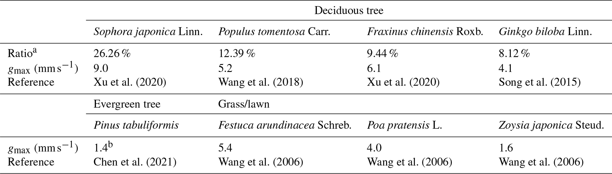

Table E1 Maximum conductance (g_max) for each vegetated surface.

^a Obtained from a field survey over Beijing (Ma et al., 2019). ^b obtained by dividing maximum canopy conductance by G₁ (= 3.5)

Appendix F: Comparison of parameters for modeling domain with different radii

Table F1 Land surface fraction for modeling domain with different radii, where “Paved” denotes paved surface, “Bldgs” denotes buildings, “EveTr” denotes evergreen trees, “DecTr” denotes deciduous trees, “Grass” denotes grassland and lawn, “Bsoil” denotes bare soil, and “Water” denotes waterbodies.

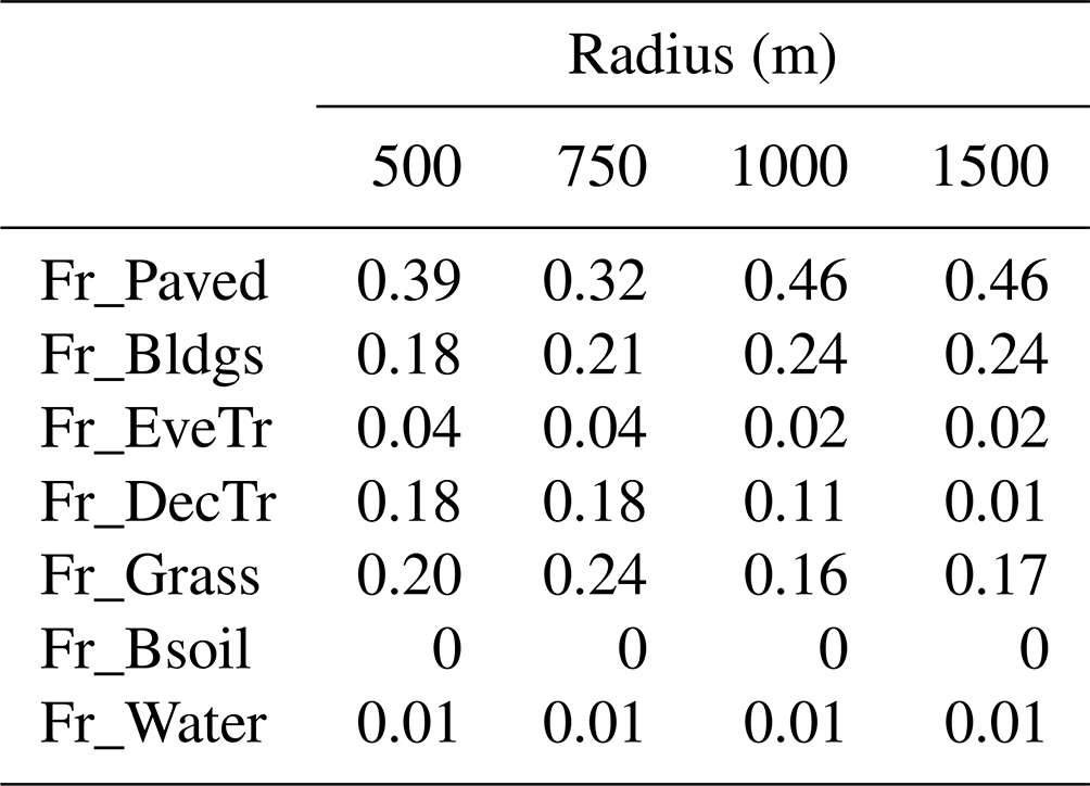
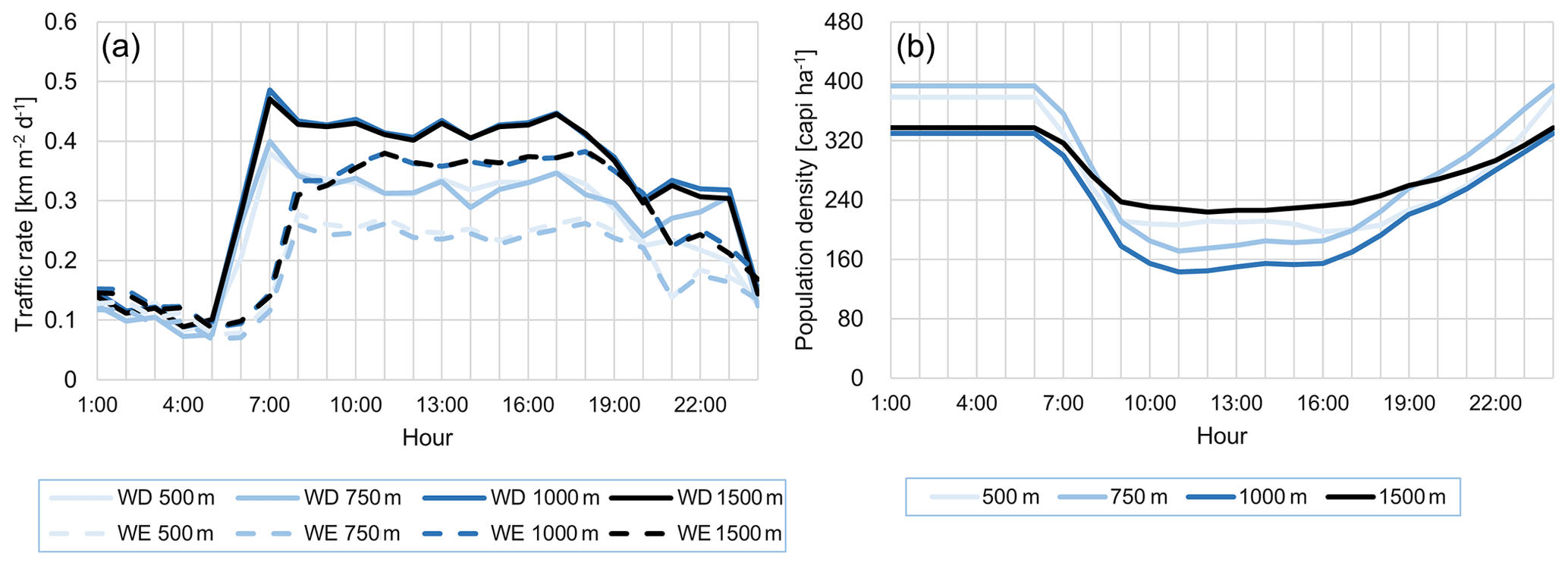
Figure F1 Diurnal cycles of (a) traffic rate and (b) population density for the modeling domain with different radii, where WD denotes weekday and WE denotes weekday.