the Creative Commons Attribution 4.0 License.
the Creative Commons Attribution 4.0 License.
 | 02 Aug 2023
A Python library for computing individual and merged non-CO2 algorithmic climate change functions: CLIMaCCF V1.0
Simone Dietmüller
Sigrun Matthes
Katrin Dahlmann
Hiroshi Yamashita
Abolfazl Simorgh
Manuel Soler
Florian Linke
Benjamin Lührs
Maximilian M. Meuser
Christian Weder
Volker Grewe
Feijia Yin
Federica Castino
Aviation aims to reduce its climate effect by adopting trajectories that avoid regions of the atmosphere where aviation emissions have a large impact. To that end, prototype algorithmic climate change functions (aCCFs) can be used, which provide spatially and temporally resolved information on aviation's climate effect in terms of future near-surface temperature change. These aCCFs can be calculated with meteorological input data obtained from, e.g., numerical weather prediction models. We present here the open-source Python library called CLIMaCCF, an easy-to-use and flexible tool which efficiently calculates both the individual aCCFs (i.e., aCCF of water vapor, nitrogen oxide (NOx)-induced ozone production and methane depletion, and contrail cirrus) and the merged non-CO2 aCCFs that combine all these individual contributions. To construct merged aCCFs all individual aCCFs are converted to the same physical unit. This unit conversion needs the technical specification of aircraft and engine parameters, i.e., NOx emission indices and flown distance per kilogram of burned fuel. These aircraft- and engine-specific values are provided within CLIMaCCF version V1.0 for a set of aggregated aircraft and engine classes (i.e., regional, single-aisle, wide-body). Moreover, CLIMaCCF allows the user to choose from a range of physical climate metrics (i.e., average temperature response for pulse or future scenario emissions over the time horizons of 20, 50, or 100 years). Finally, we demonstrate the abilities of CLIMaCCF through a series of example applications.
- Article
(7949 KB) - Full-text XML
-
Supplement
(1187 KB) - BibTeX
- EndNote


Global aviation significantly contributes to anthropogenic climate change through CO2 and non-CO2 emissions. Not all non-CO2 emissions have a direct effect on climate. Aircraft NOx emissions are not radiatively active themselves, but they are very effective in the photochemical production of ozone (O3), causing a positive radiative forcing. At the same time increased NOx and O3 concentrations lead to increased oxidation of methane (CH4), causing a negative radiative forcing (e.g., Stevenson et al., 2004; Terrenoire et al., 2022). This destruction of methane leads to a subsequent reduction in the ozone productivity, which reduces background ozone concentrations (PMO, primary-mode ozone; e.g., Stevenson et al., 2004), also causing a negative forcing. Furthermore, induced by non-CO2 emissions, contrails and contrail cirrus can form in ice-supersaturated regions and alter the radiation budget (e.g., Kärcher, 2018). Overall, as recently reviewed by Lee et al. (2021), global aviation contributes 3.5 % of the total anthropogenic radiative forcing (RF). The total aviation RF comprises about one-third CO2 effects and about two-thirds non-CO2 effects. The largest single contribution to aviation RF comes from contrails and contrail cirrus, but this estimate is affected by a very large uncertainty, as well as from NOx effects (Grewe et al., 2019). In contrast to the CO2 effect, the non-CO2 effects reveal a strong dependence on atmospheric conditions. Thus, the non-CO2 effects depend on the geographical location, altitude, and time of aircraft emission (e.g., Grewe et al., 2014; Frömming et al., 2021). In order to provide information on the spatially and temporally resolved climate effect of these non-CO2 effects, climate change functions (CCFs) were developed with an atmospheric chemistry–climate model system (Frömming et al., 2021). These CCFs provide a measure of the spatial and temporal climate effect for a given emission by using the metric of average temperature response (ATR). These CCFs were calculated for a wide range of time steps and for eight representative weather types in summer and winter classified after Irvine et al. (2013) over the North Atlantic region (Frömming et al., 2021).
Based on these CCFs, Grewe et al. (2014) investigated the transatlantic air traffic for one single winter day and analyzed the routing changes that are required to achieve a reduction in the effect of air traffic on climate. Thus, this study provides the first comprehensive and valuable basis for weather-dependent flight trajectory optimization with respect to minimum climate effect. However, as the calculation of these CCFs within a global chemistry–climate model system requires large computational cost, it cannot be used for operational climate-optimized flight planning. To address this issue, the initial concept of CCFs was extended to algorithmic climate change functions (aCCFs). These functions provide a very fast computation of the individual non-CO2 climate effect as they are based on mathematical formulas which only need a fairly limited number of relevant local meteorological parameters as input (e.g., Matthes et al., 2017; van Manen and Grewe, 2019; Yin et al., 2023). To derive the mathematical formulation of the individual aCCFs (a detailed formulation of these prototype aCCFs is given in Appendix A), statistical methods were used. A detailed explanation of the concept of the aCCF approach can be found in van Manen and Grewe (2019) for the NOx-emission-induced effect on the species ozone and methane (as NOx acts as a precursor to ozone production and methane depletion), as well as for water vapor. In the case of the contrail aCCFs approach, a detailed description is available in the Supplement of Yin et al. (2023). These aCCF formulas facilitate the prediction of the climate effect of individual species by means of meteorological input data from, e.g., weather forecast, without computationally extensive recalculation using chemistry–climate models. Of course, a number of assumptions and simplifications are necessary for this kind of statistical approach. Nevertheless, it was shown in the studies of van Manen and Grewe (2019) and Yin et al. (2023) that these prototype aCCFs are in broad agreement with the climate change metric of earlier studies, i.e., CCFs (Frömming et al., 2021).
Indeed, aCCFs can be used for trajectory planning purposes. The weather-dependent rerouting of flight trajectories in order to reduce the climate effect of air traffic needs the information on regions that are highly sensitive to aviation emissions. In order to quantify the potential of mitigating aviation's climate effect, case studies with optimized aircraft trajectories that use the aCCFs described above were performed. These studies showed that rerouting has large potential to reduce air traffic's contribution to climate change. Even small changes in the flight trajectory can lead to significant reduction of the climate effect (see, e.g., Matthes et al., 2017, 2020; Lührs et al., 2021; Castino et al., 2021; Rao et al., 2022).
Nevertheless, a climate-optimal trajectory (interested readers are also referred to Simorgh et al., 2022, for a recent, thorough survey on climate-optimal aircraft trajectory planning) requires a quantitative estimate of CO2 and non-CO2 climate effects. The latter is needed as a four-dimensional data set (latitude, longitude, altitude, time). This location- and time-dependent quantitative estimate can be generated by combining the individual aCCFs of water vapor, NOx-induced ozone (production), NOx-induced methane (depletion), and contrail cirrus into a merged non-CO2 aCCF by means of a consistent climate metric. However, for combining the individual aCCFs, it has to be considered that the aCCF algorithms provide their estimates in average temperature change per emitted mass of the relevant species, e.g., in K kg(NO2)−1, for the ozone aCCF. Thus, before merging the individual aCCFs, all individual aCCFs have to be converted to the unit of K kg(fuel)−1. For this conversion the information on NOx emission indices and flown distance per kilogram of burned fuel (specific range) is needed. Based on these generated merged non-CO2 aCCFs, climate-optimized trajectories that aim to avoid climate-sensitive regions can be calculated efficiently. Note that the total merged aCCFs (non-CO2 as well as CO2 effects included) can also be calculated; however, as the CO2 aCCF is a constant in location and time, we focus on the merged non-CO2 aCCFs.
The development of the Python library, CLIMaCCF, which will be released together with this paper (available on Zenodo with the software DOI: https://doi.org/10.5281/zenodo.6977272, Dietmüller, 2022), represents a technical enabler to seamlessly integrate information on spatially and temporally dependent non-CO2 climate effects (in terms of individual and also merged non-CO2 aCCFs) in a trajectory optimization tool. In this paper we will present both the scientific background of merging aCCFs and the technical framework of the user-friendly and flexible Python library CLIMaCCF V1.0.
The paper is structured as follows. In Sect. 2 we explain how individual aCCFs are combined into a merged non-CO2 by making assumptions about emission indices of NOx and flown distance per kilogram of burned fuel. We also provide a detailed overview of the scientific climate background needed to understand which decisions have to be made before generating the merged aCCFs. This includes insights into physical climate metrics and forcing-dependent efficacies. In Sect. 3 the technical implementation (general architecture) of the Python library CLIMaCCF is given by describing how the user can generate individual and merged aCCFs in a flexible manner. Sect. 4 provides various analyses of the individual aCCFs and the merged aCCFs, showing their characteristic patterns. Moreover, the sensitivity of merged aCCFs to different assumptions, as well as identifying regions of high climate sensitivity in the presence of aircraft emissions, is given. A discussion about the capability and limitations of the Python library follows (Sect. 5), before the conclusions are drawn in Sect. 6.
Based on aCCFs that represent the individual effects of water vapor, NOx-induced ozone increase, NOx-induced methane decrease, and contrail cirrus, a single aCCF function which combines these individual CO2 and non-CO2 effects can be generated (i.e., merged aCCFs). This merged aCCF can be used as advanced meteorological (MET) information for flight planning, as a climate-optimized trajectory requires the quantification of the total climate effect as a four-dimensional data set (latitude, longitude, altitude, and time). Such a merged aCCF can only be constructed by using assumptions on several aircraft- and engine-specific parameters as well as consistent climate metrics. In the following, we describe the concept of merging aCCFs and the underlying assumptions (choice of aircraft and engine parameters, climate metric, and efficacy) in detail.
2.1 Mathematical formulation of individual aCCFs
As mentioned in the Introduction, aCCFs were developed to provide a computationally fast way to calculate the climate effect of individual non-CO2 aviation emissions as a function of their geographical location, altitude, time, and weather. Correlations and statistical methods were used to derive the individual prototype aCCFs of water vapor, NOx-induced ozone (production), NOx-induced methane (destruction), and contrail cirrus. For water vapor, ozone, and methane aCCFs, this was done by linking a large range of climate change function (CCF) data, which were calculated in a detailed chemistry–climate model simulation (Frömming et al., 2021), to selected meteorological data, such as temperature or geopotential height (van Manen and Grewe, 2019). The algorithm for contrail aCCFs was developed differently. Contrail aCCFs are obtained from contrail radiative forcing calculations, which are based on European Centre for Medium-Range Weather Forecasts (ECMWF) reanalysis and contrail trajectory data (Yin et al., 2023). A short overview of the mathematical formulation of these emission-type-dependent prototype aCCFs is given in Appendix A of this document. For a detailed description of the first complete and consistent set of prototype aCCFs (aCCF-V1.0) the reader is referred to Yin et al. (2023). Moreover, within the EU project FlyATM4E an updated set of aCCFs (aCCF-V1.0A) was developed that considers the current level of scientific understanding of aviation's climate effects: for more details, readers are referred to Matthes et al. (2023b) and FlyATM4E-D1.2 (2023). Overall, for the development of the aCCF a number of assumptions and simplifications were necessary, e.g., in the statistical approach or in the calculation of the CCF data in a climate–chemistry model. Nevertheless, it was shown that these aCCFs are in broad agreement with the climate change metric of earlier studies (e.g., van Manen and Grewe, 2019; Yin et al., 2023).
2.2 Merged non-CO2 aCCFs and total aCCFs
To build the merged non-CO2 aCCFs, all individual aCCFs are consistently converted to the same physical units of [K kg(fuel)−1]. In order to be independent of the aircraft type the individual aCCFs (except the water vapor aCCF) are given in specific units, i.e., K km−1 for contrail aCCFs or K kg(NO2)−1 for the NOx-induced ozone and methane aCCF. By simply multiplying the NOx-induced aCCFs (, and aCCFPMO) by the NOx emission indices ( in g(NO2) kg(fuel)−1) and the contrail-cirrus aCCF (aCCFcontrail) by flown distance per kilogram burned fuel (Fkm in [km kg(fuel)−1]) all individual aCCFs are converted to the same unit (K kg(fuel)−1), and in a second step the converted individual aCCFs are combined into a merged aCCF (see Eq. 1). Note that the water vapor aCCF formula is already fuel-related and thus does not need to be multiplied by the emission index of water vapor. Typical transatlantic fleet mean values of and of Fkm are available from the literature: the transatlantic fleet mean value for Fkm is 0.16 km kg(fuel)−1 (Graver and Rutherford, 2018 and Florian Linke, TU Hamburg, personal communication, 2020) and for it is 13 g(NO2) kg(fuel)−1 (e.g., Penner et al., 1999), respectively. Another possibility is to take specific emitted amounts of NOx emissions and fuel consumption values from an engine performance model. In this study we also provide altitude-dependent mean emission indices for NOx and flown distance per kilogram of burned fuel for aggregated aircraft and engine classifications (e.g., regional, single-aisle, and wide-body; see Sect. 2.3) and combine that with the choice of climate metric (Sect. 2.4) and the use of forcing efficacies (Sect. 2.5) to merge non-CO2 aCCFs:
where aCCFX represents the algorithmic climate change functions for species X, i.e., water vapor (H2O), ozone (O3), methane (CH4), primary-mode ozone (PMO), and contrail cirrus. The variables and z indicate the three spatial variables () and time (t). iac is the identifier for three mean aircraft and engine classes: regional, single-aisle, and wide-body (see Sect. 2.3). rX(ir) is the efficacy (see Sect. 2.5) of the species X with the switch for disregarding or using the efficacies (i.e., rX(0)=1), and CMX(iCM) is the climate metric conversion factor (see Sect. 2.4) for species X and the choice of currently four climate metrics .
By additionally including the aviation climate effect of CO2 the total merged aCCF is given.
Note that the CO2 aCCF is independent of the location , efficacy (rX), and aircraft class.
For a merged aCCF it is required that the individual aCCFs are based on the same physical climate metric, emission scenario, and time horizon. The recent publication of Yin et al. (2023) comprises such a consistent set of individual updated prototype aCCFs. Note that earlier publications (e.g., Yamashita et al., 2020) provided mathematical formulations that assumed different emission scenarios for water vapor and NOx aCCFs as well as for contrail aCCFs, as they were developed separately.
Overall, merged aCCFs are a function not only of time and location, but also of aircraft- and engine-specific data, climate metric, and efficacy. For an efficient and flexible provision of such merged aCCFs we developed the Python library CLIMaCCF.
2.3 Choice of aircraft- and engine-specific parameters
The calculation of merged non-CO2 aCCFs requires knowledge about the emission index of NOx, , and the flown distance per kilogram of burned fuel, Fkm (see Eq. 1). As these indices vary depending on the actual aircraft–engine combination (iac) and the cruise altitude (z), the use of global mean emission indices should be avoided. Moreover, there is a strong altitude dependency of the NOx emission index and flown distance Fkm, which should be considered as well. Aggregated values for altitude-dependent emission indices are derived from trajectory simulation and emission inventory data. Similarly, aggregated values for the specific range (i.e., flown distance per kilogram of burned fuel) Fkm are obtained.
For instance, analyzing the 10 most frequented routes in the North Atlantic flight corridor (NAFC) with the 10 most used aircraft types in 2012 yields an average flown distance per kilogram of burned fuel of 0.16 km kg(fuel)−1 (Florian Linke, personal communication, 2020) for transatlantic flights. More differentiated values are obtained by analyzing available emission inventory data from the DLR project “Transport and Climate” (TraK). These data contain the air traffic emission distribution in the year 2015 and can be evaluated separately per aircraft type, altitude, or region. The basis for the development of these emission inventories was a database of reduced emission profiles within the Global Air Traffic Emission Distribution Laboratory (GRIDLAB, Linke et al., 2017). Those profiles were created by simulating aircraft trajectories for various ranges and load conditions with aircraft performance models from EUROCONTROL's Base of Aircraft Data (BADA, Nuic and Mouillet, 2012) model families 3 and 4. Along those trajectories engine emissions were calculated using the EUROCONTROL-modified Boeing fuel flow method 2 (DuBois and Paynter, 2006; Jelinek, 2004) applied to engine certification data for the landing and take-off cycle (LTO) taken from the International Civil Aviation Organization (ICAO) engine emission database. In order to create the reduced profiles, those trajectory emission data were finally resampled to only consider key points along the profile such as transitions between flight phases. The emission inventory contains gridded data at a resolution of 0.25∘ × 0.25∘ × 1000 ft. Associated with each grid cell are the amounts of the individual emission species as well as the flown distance in that grid cell. The aggregated mean value at a given altitude is calculated by dividing the sum of the amounts of emissions per species in all grid cells at that altitude by the sum of burned fuel at that altitude. The specific range is calculated accordingly. We evaluated aggregated fleet-level values for (iac, z) and the specific range Fkm(iac, z) for a variety of aircraft and engine classes. As the aircraft-specific values are similar for certain aircraft and engine classes, we group those aircraft classes and provide their average fleet values and their standard deviation in Tables 1 and 2. Three different aircraft types are given: regional (small aircraft with a short range, up to 100 seats), single-aisle (short- to medium-range narrow-body aircraft), and wide-body (medium- to long-range aircraft, 250–600 seats).
Table 1Average specific NOx emission indices and their standard deviation (in g(NO2) kg(fuel)−1) for the three aircraft classes (regional, single-aisle, wide-body) derived from the global TraK emission inventory. ((iac, z)) values are shown for various typical flight altitudes (20 000–40 000 ft). Besides the flight altitude in feet, the corresponding pressure level under ICAO standard atmosphere is given (hPa).
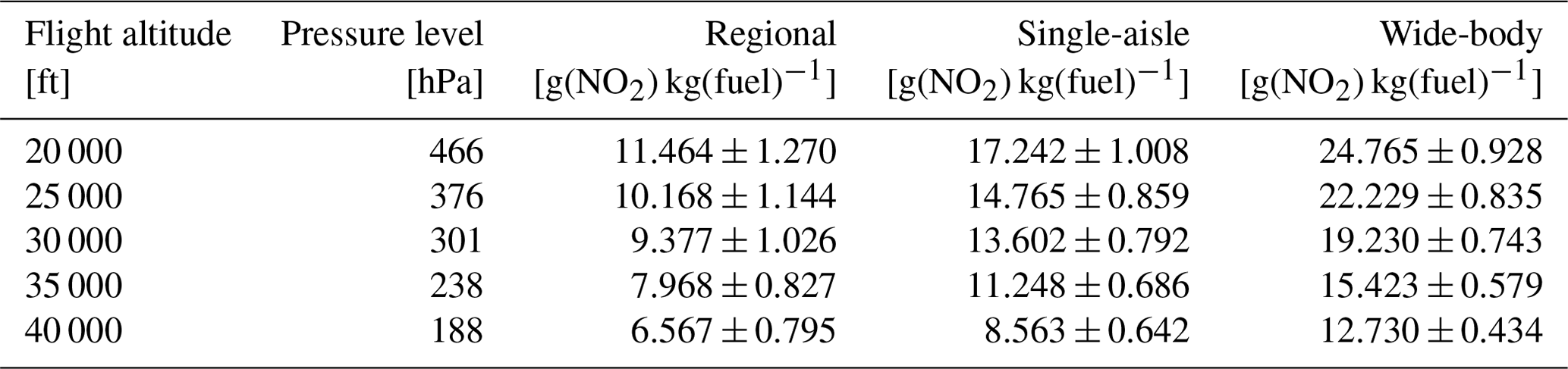
Table 2Average flown distances per burned fuel and their standard deviation (in km kg(fuel)−1) for the three aircraft classes (regional, single-aisle, wide-body) derived from the global TraK emission inventory. Fkm(iac, z) values are shown as a function of typical flight altitude (20 000–40 000 ft). Besides the flight altitude in feet, the corresponding pressure level under ICAO standard atmosphere is given (hPa).
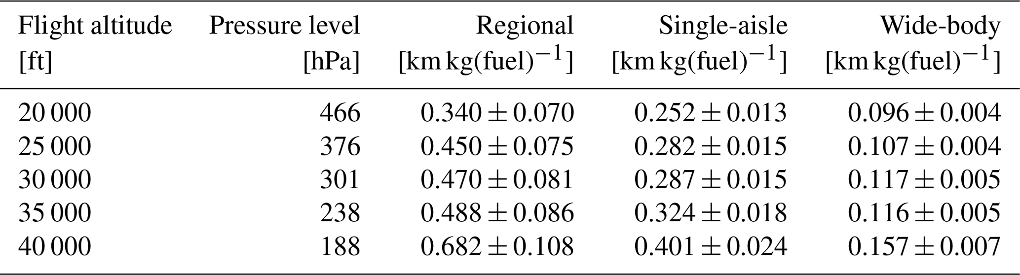
Table 1 clearly shows that average values increase with increasing aircraft class and size, while values decrease with increasing altitude. NOx emissions are produced during combustion due to high combustion temperatures, which are connected to high thrust settings and engine load conditions. In general, the thrust requirement increases with the aircraft size. Increasing the thrust requirement leads to an increase in the combustion temperature and therefore an increase in NOx emissions. Below cruise altitude, e.g., during climb, the aircraft is operated with climb thrust and during descent with nearly idle conditions, leading to higher average engine loads at lower altitudes than during cruise. The flown distance in Table 2 increases with altitude, as the aircraft is operated in nearly fuel-optimal conditions during cruise. On the other hand, larger aircraft tend to have a lower specific range than aircraft with shorter range, as they become less fuel-efficient on longer ranges, on which they have to carry additional fuel solely for the purpose of transporting a higher fuel mass over a long distance.
2.4 Choice of physical climate metric
Physical climate metrics can be understood as methods to directly compare the climate effect of different forcing agents or different sectors and sources (Fuglestvedt et al., 2010). A climate metric is a combination of a climate indicator (e.g., average temperature response – ATR – or global warming potential – GWP), time horizon (e.g., 20, 50, or 100 years), and emission scenario (Fuglestvedt et al., 2010). For the time development of aircraft emissions a pulse (emission at a certain time), sustained (emission sustained at a certain time), or future increasing (emission continue to develop) scenario might be considered (Grewe and Dahlmann, 2015). The choice of an adequate climate effect metric depends on the specific question of climate effect (e.g., what is the contribution to the current climate effect? What is the long-term climate effect?) to be answered (Grewe and Dahlmann, 2015). Thus, depending on the question different climate effect metrics should be used.
The aCCFs were developed based on the climate metric of average temperature response over a time horizon of 20 years (ATR20). The emission scenario assumed was either based on pulse emission (P) or on the future business-as-usual emission scenario (F). This inconsistency has been discovered, and a revision of the aCCFs is given in the recent publication of Yin et al. (2023). Now all direct outputs of aCCF formulas are given in P-ATR20 (ATR20 based on pulse emission). P-ATR20 may not be well suited for all questions; e.g., for the question of the climate effect reduction of steadily applying a certain routing strategy, future emission scenarios are more suitable. Thus, we introduced conversion factors CMX(iCM) (see Eq. 1) which make it possible to switch from the P-ATR20 metric (which is the basis of the aCCF-V1.0 formulas in the Appendix A) to other physical climate metrics, such as ATR based on the future emission scenario (i.e., business as usual) with different time horizons (i.e., F-ATR20, F-ATR50, or F-ATR100). To calculate these conversion factors we use the nonlinear climate response model AirClim (Grewe and Stenke, 2008; Dahlmann et al., 2016) and perform several simulations with different emission scenarios. A first set of conversion factors for four different metrics (iCM) is presented in Table 3. Note that for the conversion factor the time development of the forcing is important. As we use the impact on an annual basis the time development of O3 and H2O forcing is the same. Therefore, the conversion factors for O3 and H2O are also the same. The conversion factors of PMO and CH4 are the same, as the time development (and forcing) of PMO is coupled with the time development (and forcing) of CH4. Conversion factors for other emission scenarios and other climate indicators will be presented in an upcoming publication.
Table 3Climate metric conversion factors CMx from P-ATR20 (pulse-emission-based ATR over 20 years) to F-ATR20 (future-emission-based ATR over 20 years), F-ATR50 (future-emission-based ATR over 50 years), and F-ATR100 (future-emission-based ATR over 100 years) for water vapor, ozone, methane, primary-mode ozone (PMO), contrail-cirrus, and CO2 aCCFs.

2.5 Choice of climate-forcing-related efficacy
Radiative forcing (RF, in W m−2) describes the change in the planetary energy balance. RF is often used as a metric for comparing the global climate effect of specific forcing components (e.g., CO2, ozone, aerosols). What makes RF so useful for comparison is its empirically based linear relationship to the steady-state global mean near-surface temperature change (e.g., Forster et al., 1997). The model-dependent constant, which relates these two parameters, is the so-called climate sensitivity parameter λ (e.g., Hansen et al., 2005; Cess et al., 1989). This relation is a good approximation for many spatially homogeneously distributed climate forcing components, such as CO2. However, for radiatively active gases with a distinctly inhomogeneous structure (vertically and horizontally), like ozone change patterns from precursor emissions of the aviation sectors and contrail cirrus, the relation with the constant climate sensitivity parameter fails (e.g., Joshi et al., 2003; Stuber et al., 2005; Hansen et al., 2005). Thus, RF of some non-CO2 forcing agents may be more or less effective in changing global mean temperature per unit forcing compared to the response of CO2 forcing. As pointed out by, e.g., Rieger et al. (2017) and Richardson et al. (2019), this can be explained by the fact that such nonhomogeneous forcings trigger feedbacks that differ from those induced by CO2 (giving a climate response different from CO2). A way to account for this is to introduce a forcing-dependent efficacy parameter, which is defined as warming per unit global average forcing divided by the warming per unit forcing from CO2. By considering this efficacy (Hansen et al., 2005; Ponater et al., 2006; Lee et al., 2021), a better prediction of the expected global mean temperature change is given.
As mentioned before, aCCFs are based on the climate metric average temperature response (ATR) over a certain time horizon, a useful metric to assess the aviation-induced climate effect (Dahlmann et al., 2016). However, here ATR was calculated without taking the efficacy of the different non-CO2 forcing components into account. Integrating the efficacies rX of water vapor, ozone, methane, and contrail cirrus into the merged aCCFs (see Eq. 1) has the potential to make the predictions of aviation-induced temperature change and climate effect more reliable. Efficacies were recently summarized in Lee et al. (2021) and are shown in Table 4. The efficacy of the NOx-induced short-term ozone and NOx-induced methane is larger than 1. This means that ozone and methane RFs have a higher impact on the temperature response than CO2. However, the efficacy values provided by Lee et al. (2021) may require updates, e.g., other values for ozone efficacies were provided by Ponater (2010), using a more realistic ozone change pattern from aviation emission. Moreover, Lee et al. (2021) assume the PMO efficacy to be equal to that for methane, although the PMO change pattern is largely unknown and there are no dedicated PMO climate sensitivity simulations available. For contrails, the efficacy given in Lee et al. (2021) is lower than 1, meaning that contrail RF has a lower impact on the global temperature response than CO2. Note that the contrail efficacy of 0.42 in Lee et al. (2021) is based on three different contrail efficacy estimates from earlier studies, including an estimate of 0.59 (Ponater et al., 2005), an estimate of 0.31 (Rap et al., 2010), and an estimate of 0.35 (Bickel et al., 2020). Efficacies strongly deviating from unity (as in the case of contrail cirrus) can substantially affect the assessment of mitigation measures (e.g., Deuber et al., 2013; Irvine et al., 2014), but it would be desirable to have more model studies on the subject to establish more reliable values.
Ponater et al. (2006)Ponater et al. (2006)Lee et al. (2021)Lee et al. (2021)Ponater et al. (2005)Rap et al. (2010)Bickel et al. (2020)Lee et al. (2021)Table 4Overview of efficacies rX of NOx-induced ozone, methane, PMO, water vapor, and contrail cirrus. Respective references are given on the right side of the table.
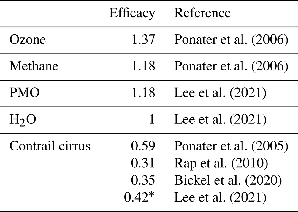
* The Lee et al. (2021) value is the mean over the values given by Bickel et al. (2020), Ponater et al. (2005), and Rap et al. (2010).
The generation of individual and merged non-CO2 aCCFs will be performed by using a user-friendly library developed with Python, called CLIMaCCF. The scope of CLIMaCCF is to provide individual and merged aCCFs as spatially and temporally resolved information considering meteorology from the actual synoptical situation, the engine and aircraft type, the selected physical climate metric, and the selected version of prototype algorithms in individual aCCFs (i.e., aCCF-V1.0 and aCCF-V1.0AQ; see Sect. 2.1). In the following, some details on the technical implementation of the Python library are presented. For more comprehensive documentation, the reader is referred to the CLIMaCCF user manual that is provided as a Supplement to this paper. Overall, the Python library consists of three main blocks: input block, processing block, and output block (see the schematic workflow in Fig. 1). In the input block, the Python library obtains the weather data (e.g., forecast, reanalysis) containing the required meteorological input and configurations like the climate metric as well as the aircraft and engine class. In the processing block, the individual aCCFs are calculated and merged aCCFs are generated. In the output block the individual and merged aCCFs are stored. In the following we describe these three blocks in more detail.
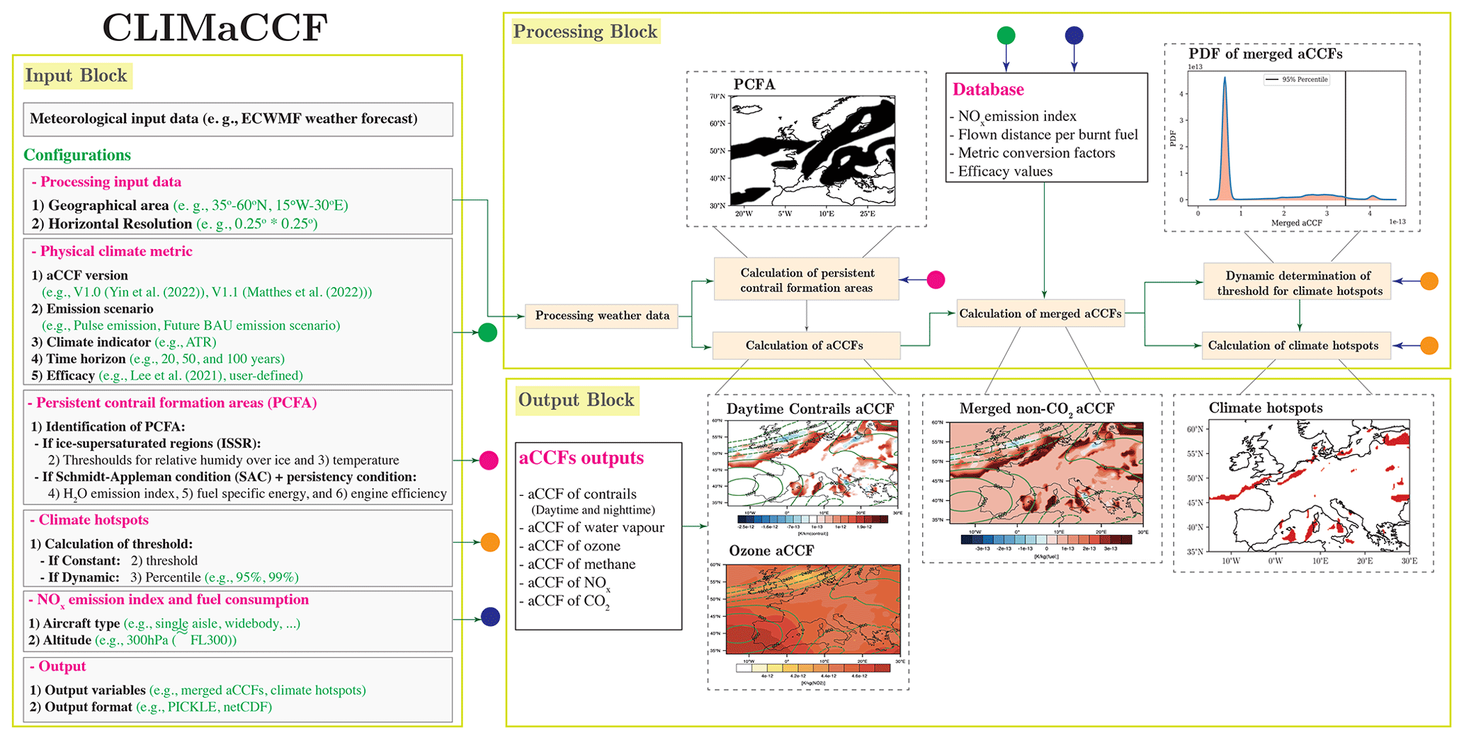
Figure 1Schematic workflow of calculating individual and merged aCCFs using the Python library CLIMaCCF version 1.0. The left box describes the input block, the upper right box the processing block, and the lower left box the output block.
3.1 Input block
Within the input block (left box in Fig. 1), the meteorological input data needed to calculate aCCFs are specified by the user. All meteorological input data needed to calculate the individual aCCFs are summarized in Table 5. The current implementation of the library is compatible and tested with several data products of the European Centre for Medium-Range Weather Forecasts (ECMWF) (i.e., reanalysis data ERA5 and ERA-Interim, forecast). These user settings include the selections of geographical area, horizontal resolution, and several output options (e.g., the output file can include merged aCCFs, individual aCCFs, and the input data used). Besides the specification of meteorological input data, users can select the version of aCCFs they aim to use. These options include aCCF-V1.0, which is the first consistent and complete set of aCCFs (Yin et al., 2023), aCCF-V1.0A, in which the aCCF-V1.0 is calibrated to the climate response model AirClim (see Matthes et al., 2023b; FlyATM4E-D1.2, 2023). Additionally user-defined scaling factors can be applied to the selected aCCF version. These scaling factors are set to 1 by default; however, if a scaling of the aCCFs (to higher or lower values) is desired (e.g., for sensitivity studies) the user can adopt them accordingly. User settings for the generation of individual and merged aCCFs can also be selected. Here, the user can choose different assumptions for aircraft-specific parameters and the physical climate metric (emission scenario, physical climate indicator, time horizons). Moreover, the user can decide if the aCCF calculation is performed with or without consideration of efficacy. As for efficacy, users can use the values reported by Lee et al. (2021) or use efficacy values provided by other studies. As the selection of aircraft and engine classification is an important factor in determining reliable merged aCCF (see Sect. 2), we have implemented an initial set of specific emission indices for some selected aircraft–engine combinations. By selecting an aggregated aircraft and engine type, tabulated flight-level-dependent NOx emission indices and flown distance per burned fuel values are used to calculate the merged aCCFs. An additional functionality is the identification of areas that are very sensitive to aviation emission, in the following called “climate hotspots”. To quantify these areas, a threshold value is used to identify the regions with very large effects induced by aviation. The threshold to determine these climate hotspot areas is also considered an adjustable parameter (for details, see Sect. 4). In the end, the users can specify output parameters such as merged aCCFs or the aCCFs of each species. In the case of using ensemble forecasts, one can also receive the ensemble mean and ensemble spread of the resulting individual or merged aCCFs from CLIMaCCF. The user can select the output format (either netCDF or PICKLE). There is also a possibility to output the climate hotspots in the GeoJSON file format.
3.2 Processing block
The processing block (upper right box in Fig. 1) performs the aCCF calculations using the given weather data and the user settings described above. The processing block includes, for the aCCF calculation, preprocessing of input variables, the calculation of individual and merged aCCFs, and the calculation of climate-sensitive regions (climate hotspots). A more detailed description of these calculations is given in the following.
Before calculating individual and merged aCCFs, preprocessing of several input data is needed.
-
Processing weather data. In an initial step, based on the user preferences, the geographical areas where the merged aCCFs are calculated can be reduced, or the default resolutions can be changed. In these cases, some modifications are applied to the original input weather data. Notice that the horizontal resolution cannot be increased, and the decrease in resolution is a factor i of natural numbers. For instance, if the resolution of meteorological input data is 0.25∘ × 0.25∘, the resolution can be reduced to for i∈ℕ.
-
Calculate required weather variables form alternative variables. If some required meteorological variables are missing in the input data set, they can be retrieved from alternative variables included in the data set, but only if alternative variables described in Table 5 exist in the data set, as they will be employed to calculate the required variables.
-
Tabulated aircraft- and engine-specific parameters. In the database of the library, NOx emission indices () and flown distances (Fkm) are provided for different types of aircraft (i.e., regional, single-aisle, wide-body) at different flight levels. By using spline interpolations, these indices are calculated for any given flight level (or pressure level).
-
Calculate persistent contrail formation areas. The units of the daytime and nighttime contrail aCCFs are [K km−1], meaning that they are defined only in areas where the formation of persistent contrails is possible, called persistent contrail formation areas (PCFAs). These regions are identified by two atmospheric conditions (e.g., Gierens et al., 2020): first, the Schmidt–Appleman condition (SAC) (Appleman, 1953), stating that contrails form if the exhaust–air mixture in the expanding plume reaches water saturation, has to be fulfilled. SAC describes the formation of both short-lived and long-lasting (or persistent) contrails. For the persistence of contrails a second criteria is needed: the ambient air has to be supersaturated with respect to ice, meaning that the relative humidity over ice (rhumice) is higher than 100 %. Within CLIMaCCF the PCFAs are calculated in the processing step. Here the user has two possibilities: the first possibility is to calculate PCFA by using the thresholds of ice-supersaturated regions (ISSRs) with the temperature threshold of T<235 K and the threshold of relative humidity over ice >100 % (see the Supplement of Yin et al., 2023) (PCFA-ISSR). The second possibility, which is more accurate, is to calculate SAC explicitly to define the temperature threshold and then additionally assume ice supersaturation (PCFA-SAC). Note, however, that for the exact calculation of SAC, parameters of aircraft and engine properties are also needed.
-
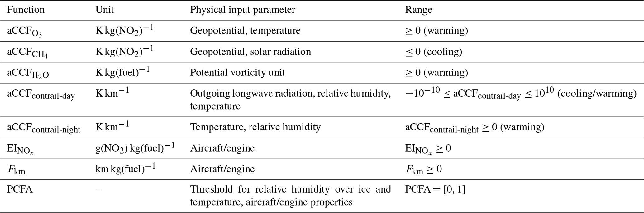
The calculation of the individual and merged aCCFs within CLIMaCCF is based on the aCCF formulas of Yin et al. (2023) (see Appendix A). By using the provided original and preprocessed input data the individual and merged aCCFs are calculated. Moreover, user-specific conversion factors due to the selected physical climate metric, efficacy, and aircraft-specific emission indices are needed. Table 6 summarizes all the individual aCCFs and parameters needed to calculate merged aCCFs. Additionally the processing block includes the calculation of climate hotspots, areas that are very sensitive to aviation emissions. The calculation of climate hotspots is based on the calculated merged aCCFs. To identify these climate hotspots a threshold based on the merged aCCFs is needed. This threshold can either be fixed to a user-defined parameter or determined dynamically within CLIMaCCF by calculating the percentile value (e.g., 90 % or 95 %) of the merged aCCF (a more detailed explanation of the dynamical approach is given in Sect. 4).
3.3 Output block
In the output block (lower right box in Fig. 1), the processed aCCFs are saved. In the current version, for saving aCCFs (e.g., individual aCCFs, merged aCCF, and climate hotspots) and weather variables (if selected), NetCDF and PICKLE file formats can be selected. In addition, the user can choose the GeoJSON format for storing polygons of climate-sensitive regions (i.e., climate hotspots).
Table 5Meteorological variables and their alternatives needed to calculate aCCFs.
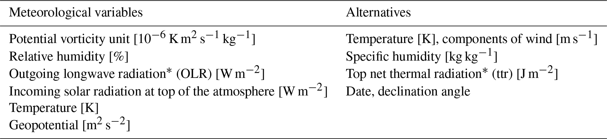
* Values of OLR and ttr have to be negative.
The Python library CLIMaCCF allows easily generating output of the spatially and temporally resolved climate effect of aviation emissions by using available aCCFs. As mentioned above the individual aCCFs of NOx-induced ozone and methane, water vapor, and contrail cirrus, as well as the merged non-CO2 aCCFs, can be calculated with CLIMaCCF. In this section, we describe different characteristic patterns of individual and merged aCCFs over the European airspace. We use the aCCFs over the whole European airspace (although they were developed over the NAFC), as weather pattern analysis showed that Europe is highly influenced by North Atlantic dynamics. We also compare merged aCCFs using different assumptions of aircraft types and metrics, and we explain how to identify regions that are very sensitive to aviation emissions (so-called climate hotspots) and how these climate hotspots behave.
The meteorological input data used for calculating the aCCFs within the CLIMaCCF were taken from the ERA5 high-resolution realization reanalysis data set (Hersbach et al., 2020). ERA5 is the fifth generation of the European Centre for Medium-Range Weather Forecasts (ECMWF) atmospheric reanalysis. ERA5 high-resolution (HRES) data are archived with a horizontal resolution of 0.28∘ × 0.28∘.
Table 6The functions and variables needed to calculate merged aCCFs.
4.1 Analysis of individual and merged aCCFs by using the Python library CLIMaCCF
As an application example we show typical summer patterns of water vapor, NOx-induced (including ozone, methane, and PMO), contrail-cirrus, and merged non-CO2 aCCFs at 12:00 UTC (under daytime conditions) on 15 June 2018 over the geographical region of Europe (15∘ W–30∘ E, 35–60∘ N) at a pressure level of 250 hPa. With this analysis we aim to give an impression of the typical structure and of gradients of the specific aCCFs over the European airspace. Note that in this subsection, we generated individual and merged aCCFs using aCCF-V1.0A and by assuming the climate metric of F-ATR20 with inclusion of efficacies. For merging we used typical transatlantic fleet mean parameters (see Sect. 2). In the case of merged aCCFs we will focus on the merged non-CO2 aCCFs (Eq. 1), as the merged aCCF pattern does not change if including the CO2 aCCF, which has a constant value in time and location. But of course, for climate-optimal trajectory optimization, fuel consumption also has to be taken into account, as this is directly linked to CO2 emissions.
4.1.1 Water vapor aCCF
Figure 2 presents the typical water vapor aCCFs over Europe for the specific summer day. As aircraft-induced water vapor emissions have a warming effect, the water vapor aCCFs reveal positive values in all regions. The values of water vapor aCCF are highly variable, and they vary with location by a factor of about 3. This regional variation in the aCCFs pattern highly follows the weather pattern; the maximum value can be observed over the region with negative geopotential height anomalies (see overlaid green lines), indicating low pressure and a low tropopause.
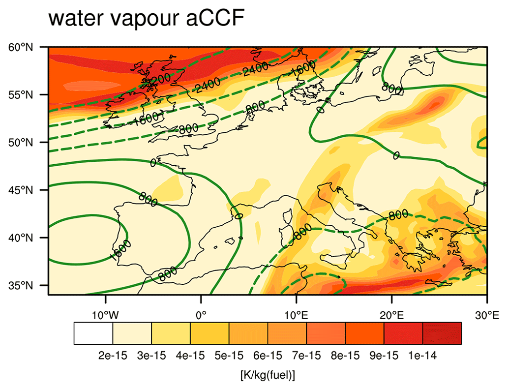
Figure 2Water vapor aCCF at a pressure level of 250 hPa over Europe at 12:00 UTC on 15 June 2018. Units are given in [K kg(fuel)−1]. Overlaid green lines indicate positive (solid line) and negative (dashed line) geopotential height anomalies (in m2 s−2).
4.1.2 NOx-induced aCCFs
To better understand the total NOx-induced aCCF, the NOx aCCF is displayed in Fig. 3 together with the ozone and methane aCCF. Note that the long-term primary-mode ozone (PMO) is included here in the methane aCCF. The ozone aCCF (Fig. 3a) is positive (warming), as NOx emissions from aviation induce the production of the greenhouse gas ozone. It reveals generally higher values in southern regions, as photochemical ozone formation increases with the availability of sunlight as well as with temperature. Additionally, the synoptical weather pattern influences the ozone aCCF values, as emitted NOx that is transported to lower latitudes experiences more solar radiation, and thus photochemical ozone production is higher compared to that which remains at higher latitudes. The methane aCCF is negative (Fig. 3b), as NOx emissions cause a decrease in methane concentrations, as there is a decrease in warming from methane. The resulting total NOx aCCF (Fig. 3c), a combination of ozone warming and methane net cooling effects, reveals that the ozone effect dominates the overall warming effect of NOx emissions. Note that by using the metric of ATR20 and an underlying future emission scenario, the differences in lifetime between NOx, ozone, and methane are taken into account.
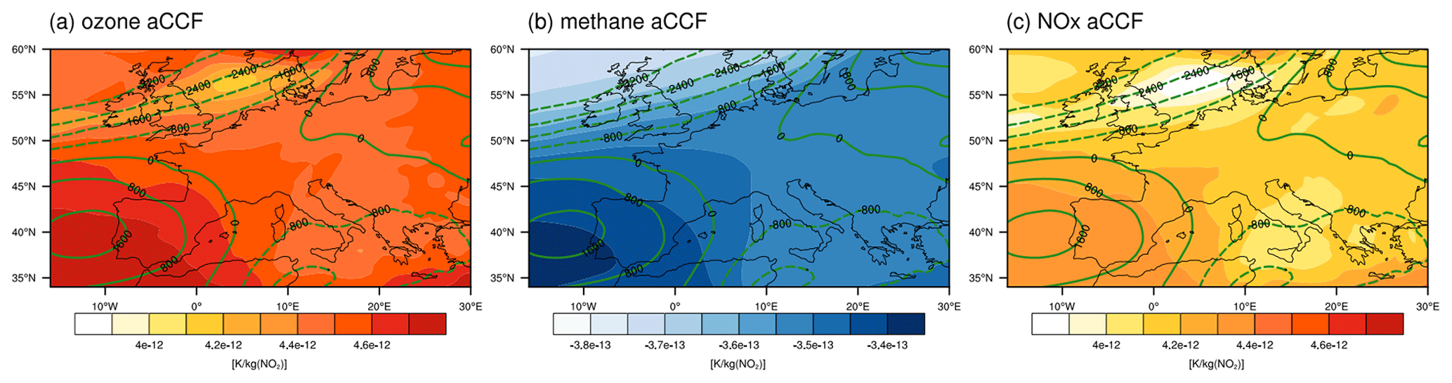
Figure 3(a) Ozone aCCF, (b) methane aCCF (including PMO), and (c) total NOx aCCF (sum of ozone, methane, and PMO aCCFs) at a pressure level of 250 hPa over Europe at 12:00 UTC on 15 June 2018. Units are given in [K kg(NO2)−1]. Overlaid green lines indicate positive (solid line) and negative (dashed line) geopotential height anomalies (in m2 s−2).
4.1.3 Contrail-cirrus aCCFs
Only if the atmospheric conditions allow for a contrail formation is the contrail aCCF nonzero. Figure 4 shows the daytime contrail-cirrus aCCF that can lead to either a positive or negative climate effect. Whether the climate effect is positive or negative depends mainly on the solar insolation, as contrails not only reduce the outgoing longwave radiation (warming) but also reflect the shortwave incoming radiation (cooling). The spatial variability in the contrail aCCF is very high and ranges from zero (regions with no persistent contrail formation) to high positive or negative values. This is clear as the formation of persistent contrails is highly sensitive to the actual atmospheric conditions.
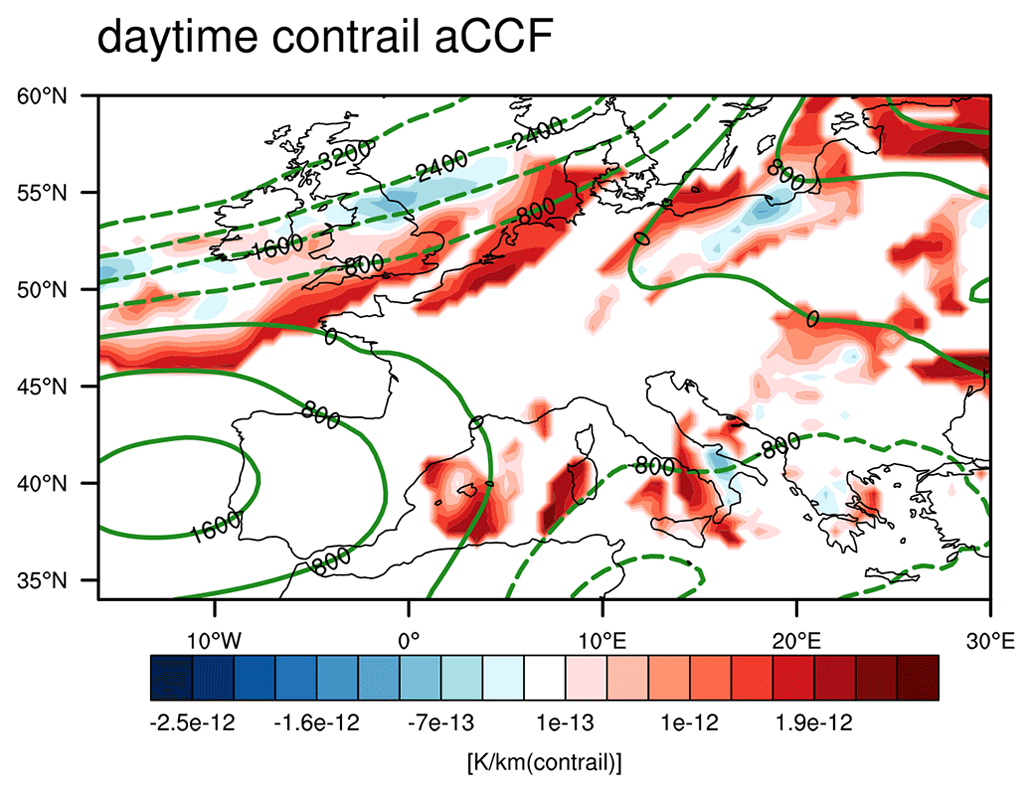
Figure 4Daytime contrail aCCF at a pressure level of 250 hPa over Europe at 12:00 UTC on 15 June 2018. Units are given in [K km−1]. Overlaid green lines indicate positive (solid line) and negative (dashed line) geopotential height anomalies (in m2 s−2).
4.1.4 Merged non-CO2 aCCFs
Figure 5 shows the merged non-CO2 aCCF, which combines the water vapor, NOx-induced, and contrail-cirrus aCCFs. The shown merged aCCF is calculated based on the climate metric of F-ATR20, taking into account the different efficacies of contrails, ozone, and methane. Moreover, the typical averaged fleet mean values of transatlantic flights are taken for the NOx emission index and the specific range. The comparison of the individual aCCF components (see Figs. 2–4) with the merged non-CO2 aCCF (Fig. 5) clearly shows that the contrail-cirrus aCCF dominates the non-CO2 climate effect in the regions where contrails form. By converting all the individual aCCFs to the same unit (K kg(fuel)−1), the direct comparison of the aCCFs can be allowed (see Appendix B, Fig. B2 first row). This shows that contrail aCCFs have the highest climate effect in the contrail formation areas, followed by the NOx-induced aCCF, whereas the water vapor aCCF is of negligible magnitude in this case. Thus, adding the high values of the positive contrail aCCF to the smaller positive NOx aCCF values leads to very high values in the merged aCCF, whereas areas of negative contrail aCCF mostly lead to the negative merged aCCF, as the magnitude of the negative aCCF is often higher than that of the NOx-induced aCCF. On the basis of the merged aCCF (Fig. 5), a hypothetical climate-optimized European flight (which will stay on this pressure level for simplification) would certainly try to avoid the areas with high positive merged aCCFs. Further, this flight trajectory will probably find a compromise between avoiding long distances through enhanced climate warming areas and at the same time avoiding long detours as these would induce a penalty with respect to CO2 aCCF. Thus, if the trajectory is optimized based on the merged non-CO2 aCCF, this penalty is not taken into account.
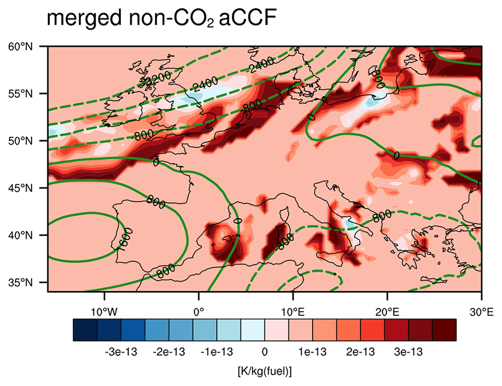
Figure 5Merged non-CO2 aCCF at a pressure level of 250 hPa over Europe at 12:00 UTC on 15 June 2018. Units are given in [K kg(fuel)−1]. Overlaid green lines indicate positive (solid line) and negative (dashed line) geopotential height anomalies (in m2 s−2).
4.2 Sensitivity of merged aCCFs to different aircraft and aircraft classes as well as climate metrics
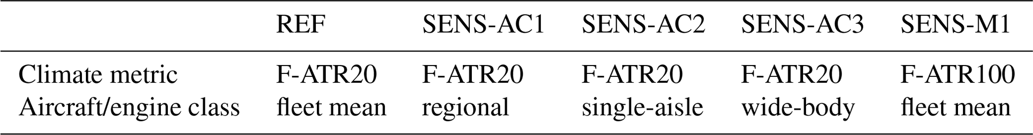
As mentioned above, the merged aCCFs can be used as advanced MET information for flight planning, as CLIMaCCF enables quantifying the total non-CO2 climate effect as a four-dimensional data set (latitude, longitude, altitude, and time) that is necessary for a climate-optimized trajectory. In Sect. 4.1, we showed the merged aCCF constructed with CLIMaCCF assuming the climate metric of F-ATR20 (the efficacies included) as well as the transatlantic fleet mean value of the NOx emission index and the specific range. However, as described in Sect. 2, there are several choices for generating the merged aCCFs. These choices are related to the climate objective (climate metric) and the emission behavior of the aircraft type, and they depend of course on a user objective. In the following, we investigate how sensitive the merged non-CO2 aCCFs are to different assumptions. Table 7 summarizes the different considerations of merged non-CO2 aCCFs that were performed with CLIMaCCF. The reference calculation is the same as shown in Sect. 4.1 (using the climate metric F-ATR20, inclusion of efficacies, and emission indices of typical fleet mean values of transatlantic flights). Additionally, we conducted three sensitivity calculations with height-dependent emission indices and specific ranges of different aircraft types (i.e., regional, single-aisle, and wide-body), as well as one sensitivity calculation with a different climate metric of F-ATR100.
Table 7Overview of the conducted calculations of merged non-CO2 aCCFs. Besides the reference calculation (REF), which uses transatlantic fleet mean values, there are three sensitivity calculations using height-dependent aircraft and engine parameters (i.e., , Fkm) of different aggregated aircraft types (SENS-AC1, SENS-AC2, and SENS-AC3) as well as one sensitivity calculation using a different climate metric (SENS-M1). Efficacy is taken into account for all simulations.
In the first three sensitivity calculations (SENS-AC1, SENS-AC2, and SENS-AC3), we varied the emission indices by using different aircraft types. By choosing different aggregated aircraft types (i.e., regional, single-aisle, and wide-body), the respective values of Fkm and were used (see Tables 1 and 2). Note, moreover, that, in contrast to the mean fleet value used for the reference calculation, and specific range values are flight-altitude-dependent. These sensitivity calculations are used to investigate how the aircraft type influences the overall climate effect in terms of the average temperature change. Figure 6 shows the merged aCCFs for the reference calculation (REF) and for the aircraft-dependent sensitivity calculations (SENS-AC1, SENS-AC2, and SENS-AC3) on 15 June 2018 at a pressure level of 250 hPa. Additionally, Fig. B1 in Appendix B provides aircraft- and engine-dependent merged aCCF patterns together with the respective water vapor, NOx, and contrail-cirrus aCCFs, all given in the same unit (K kg(fuel)−1). Generally, for all aggregated aircraft types, the highest climate effect is found in the areas of contrail formation. Comparing the aircraft-type-dependent merged aCCFs reveals that contrails are more dominant for the regional and single-aisle aircraft types. In the case of regional (SENS-AC1) and single-aisle (SENS-AC2) aircraft types, the merged aCCFs have very high contrail aCCF values (see Fig. B1), leading to the high absolute merged aCCF values. The maximum merged aCCF values are smaller if the transatlantic fleet mean (REF) and the wide-body (SENS-AC3) aircraft type emission indices are chosen. Moreover, in regions where no contrails form, the NOx-induced aCCF (i.e., the sum of the ozone, methane, and PMO aCCFs) shows relatively high values for REF and SENS-AC3 compared to those for SENS-AC1 and SENS-AC2. Compared to the aircraft- and engine-dependent NOx emission indices and flown distances at a flight altitude of 35 000 ft (roughly corresponding to the pressure layer of 250 hPa) in Tables 1 and 2, these differences can be explained: at this cruise altitude the aggregated regional aircraft type shows the lowest (7.968 g(NO2) kg(fuel)−1) but the highest flown distance values Fkm (0.488 km kg(fuel)−1).
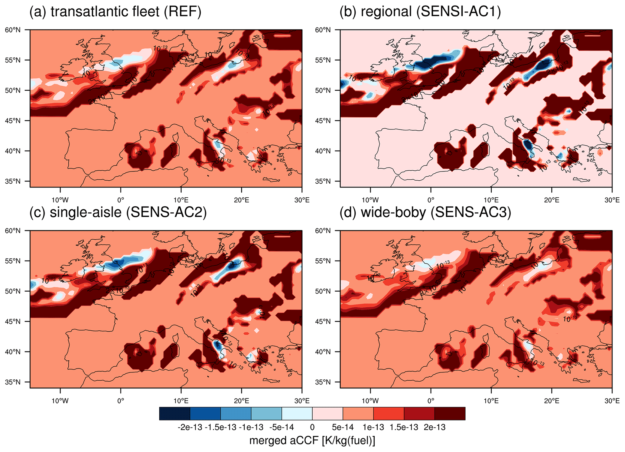
Figure 6Merged non-CO2 aCCF at a pressure level of 250 hPa over Europe on 15 June 2018 (12:00 UTC) using four different assumptions for the NOx emission index and the flown distance values: (a) typical transatlantic fleet mean, (b) regional aircraft type, (c) single-aisle aircraft type, and (d) wide-body aircraft type. Units are all given in [K kg(fuel)−1].
To generate a merged non-CO2 aCCF, it is necessary to choose a consistent climate metric for all individual aCCFs. As mentioned in Sect. 2.4, there are many metrics used in the literature to assess the climate effect; however, the choice of the metric depends on the objective of the study (e.g., Grewe and Dahlmann, 2015). CLIMaCCF provides the possibility to choose between a set of different climate metrics. Thus, we can show how different metrics influence the merged non-CO2 aCCF. As an example we compare the reference calculation (REF), which is based on F-ATR20 (Fig. 7a), to the SENS-M1 calculation, which assumes the climate metric of F-ATR100 (Fig. 7b). For the F-ATR100 metric, the focus lies more on long-term mitigation effects, whereas the choice of the F-ATR20 metric focuses on the short-term mitigation effect. Choosing the time horizon of 100 years for the F-ATR largely impacts the absolute values of the merged aCCF, as the metric conversion factor of all species is higher for F-ATR100 (see Table 3). Moreover, in Fig. B2 (Appendix B) the individual aCCFs for these two metrics are shown in terms of the same unit (K kg(fuel)−1), and we see that the climate effect of NOx-induced emissions gets more important compared to the contrail aCCFs in the case of ATR100.
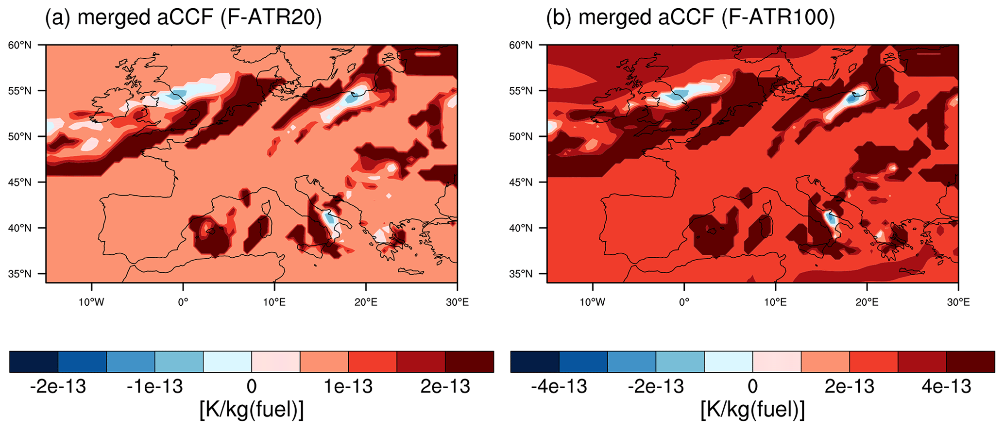
Figure 7Merged non-CO2 aCCF at a pressure level of 250 hPa over Europe at 12:00 UTC on 15 June 2018 using two different assumptions for the climate metric: (a) F-ATR20 (REF) and (b) F-ATR100 (SENS-M1).
4.3 Identification of climate-sensitive regions (climate hotspots)
Any trajectory planning tool capable for planning climate-optimized aircraft trajectories (see Simorgh et al., 2022) can use the information on the location-, altitude-, and time-dependent climate effect of non-CO2 emissions and aim to avoid such highly sensitive regions by planning for an alternative, climate-optimized, or eco-efficient aircraft trajectory. CLIMaCCF offers the possibility to identify regions with a large climate effect, called climate hotspots. Threshold values that define these climate hotspots have to be provided. These threshold values are based on the merged non-CO2 aCCF values: if the merged aCCF exceeds a certain threshold value of the merged aCCF the region is defined as a climate hotspot. As the merged aCCFs highly vary with season, flight altitude, geographical latitude, daytime and nighttime conditions, and synoptic weather situation, these threshold values should be determined dynamically for every time step and flight altitude over a certain geographical region (e.g., European airspace). To do so, we calculate the percentile (e.g., 95th percentile) of the merged aCCF distribution over all grid points spanning, e.g., the European airspace (in our example we use the geographical region of 35–60∘ N, 15∘ W–30∘ E). This percentile then provides the time step and level-dependent threshold of the merged aCCF. As mentioned above, regions are defined as climate hotspots if the corresponding merged aCCF lies above this threshold. Thus, e.g., in the case of the 95th percentile the highest 5 % of the merged aCCFs are declared as climate hotspots. In CLIMaCCF the user has the possibility to select the geographical region over which the percentile of the merged aCCF is calculated as well as the percentage (e.g., 90 %, 95 %) of the percentile.
Figure 8 illustrates such climate hotspots (in red) over the European airspace at the different cruise altitudes of 200, 250, and 300 hPa for 15 June 2018 at 12:00 UTC. The underlying merged non-CO2 aCCF used here is based on the REF calculation (see Table 7 and Fig. 5). By selecting the 95th percentile for the calculations we get different threshold values for different altitudes: K kg(fuel)−1 for 200 hPa, K kg(fuel)−1 for 250 hPa, and K kg(fuel)−1 for 300 hPa. The threshold at 250 hPa has the highest value, meaning that aviation's climate effect (in terms of merged non-CO2 aCCFs) is generally larger here. Comparing the climate hotspot patterns in Fig. 8, it is clear that these regions vary a lot for different altitudes.
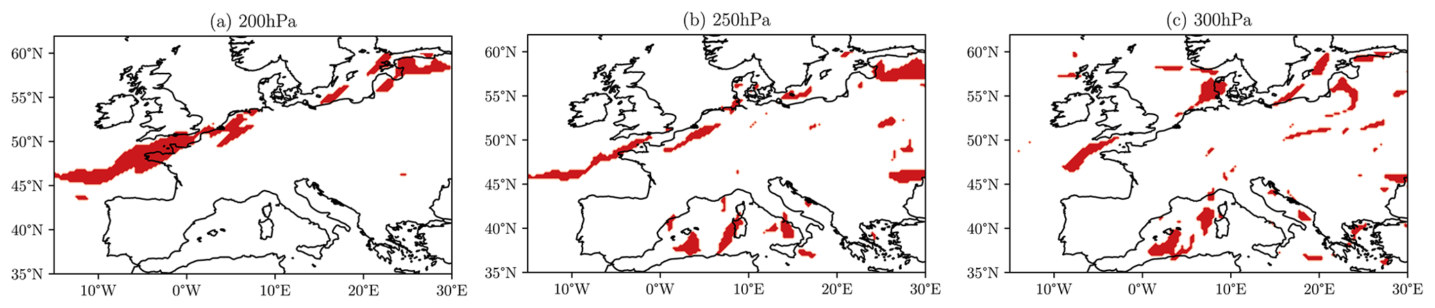
Figure 8Climate hotspots over the European airspace on the 15 June 2018 (12:00 UTC) for the flight altitudes (a) 200 hPa, (b) 250 hPa, and (c) 300 hPa. The thresholds are based on the respective (pressure-level-dependent) 95th percentile of the merged non-CO2 aCCF.
5.1 CLIMaCCF configuration
With the open-source Python library CLIMaCCF we provide a simple and easy-to-use framework for quantifying the spatially and temporally resolved climate effect of aviation emissions by making use of the aCCFs that are published in the studies of van Manen and Grewe (2019), Yamashita et al. (2020), Yin et al. (2023), and Matthes et al. (2023b). CLIMaCCF is easy to install and to run, and it efficiently calculates the individual and merged non-CO2 aCCFs, taking the actual meteorological situation into account. Merged non-CO2 aCCFs are generated by combining the individual aCCFs of water vapor, NOx-induced ozone, methane, and contrail cirrus by making assumptions on the technical specification of the engine–aircraft combination (i.e., and Fkm) and on an appropriate physical climate metric. With this newly developed Python library, the user has the possibility to investigate merged aCCFs for three different aggregated aircraft types (regional, single-aisle, wide-body) that provide flight-level-dependent values of and Fkm (for details see Tables 1 and 2). This novel feature of calculating merged aCCFs by considering the flight-level- and aircraft-dependent values of and Fkm, rather than using the transatlantic fleet mean values, leads to a better representation of aviation's non-CO2 climate effect. Compared to the study of Frömming et al. (2021), which showed aviation's merged climate effect (in terms of CCFs) by using transatlantic fleet mean values, this is a real improvement, as merged aCCFs vary significantly for different aircraft types as also shown in Fig. 6.
Moreover, CLIMaCCF offers the possibility to calculate aCCFs for a set of different physical climate metrics. For instance, the user has the flexibility to calculate the aCCFs for the climate metric of global average temperature response (ATR) with pulse emission or future emission scenario over the time horizons of 20, 50, and 100 years. However, we want to point out here that any optimization study has to carefully choose an adequate physical climate metric (i.e., its climate indicator, emission scenario, and time horizon) so that it is suitable for the specific application, which depends on strategic decisions, on given constraints, and on policy assumptions (e.g., Fuglestvedt et al., 2010; Grewe and Dahlmann, 2015). For example, a pulse emission compares the future climate effect in a given year, whereas a future emission scenario compares the effect of increasing emissions over a future time period. This leads to different estimates of the ATR, as also shown in Fig. 7.
5.2 Threshold of relative humidity for ice-supersaturated regions (ISSRs)
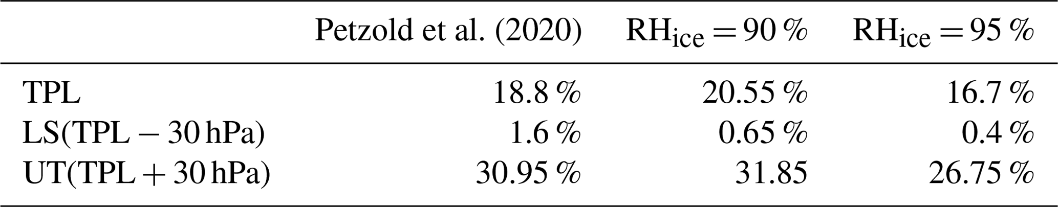
Besides the wise selection of an appropriate climate metric, other configuration parameters also have to be chosen carefully by the user. Thus, if using the Python library CLIMaCCF for calculating the climate effect of contrails the user has to pay special attention to defining the threshold of relative humidity for ice-supersaturated regions (ISSRs). In the case of contrail aCCFs we need to determine these ISSRs, as persistent contrails can only form in these regions, and the contrail aCCF is calculated only for these regions. These ISSRs are identified by two conditions: the temperature is below 235 K (in order to avoid identification of mixed-phase regions Pruppacher et al., 1998), and the relative humidity with respect to ice (RHice) exceeds 100 % (see, e.g., Yin et al., 2023, their Supplement on contrail aCCFs). However, for considering the sub-grid-scale variability in the relative humidity field in numerical weather forecast model data, e.g., ERA5, RHice thresholds below 100 % are needed. For example, Irvine et al. (2014) showed that the relatively coarse resolution of the ERA-Interim data leads to a grid box with a grid mean humidity slightly below 100 %, as it is likely within this grid box that some air parcels show relative humidity values above 100 %. In the following we explain how we derive the threshold value of RHice in order to consider the sub-grid-scale variability for the data product ERA5 HRES (see Sect. 4). To do so we calculated the annual mean (2009–2010) ISSR frequency over the European region (5∘ W–30∘ E, 40–60∘ N) using the ERA5 data set. For the ISSR frequency calculation we varied the threshold value of RHice (i.e., taking 90 % and 95 %), but leaving the temperature threshold of 235 K constant, and compared the results to the observationally based ISSR frequency values of the study of Petzold et al. (2020). This study used in situ measurement data for temperature and RHice from the full MOZAIC program1 over the period 1995–2010. Table 8 summarizes the results of our ERA5-based ISSR calculations together with the results of Petzold et al. (2020) obtained by observational data. The frequency of ISSR in the European area is shown for three different vertical levels, the tropopause layer (TPL, thermal tropopause), the upper troposphere (UT, 30 hPa below thermal tropopause), and the lower stratosphere (LS, 30 hPa above thermal tropopause). From this table we see that by setting the RHice threshold value to 90 % for ERA5 the ISSR values of Petzold et al. (2020) are best matched. Thus, taking RHice threshold values of 90 %, the ISSR frequency of Petzold et al. (2020) is only slightly overestimated in the TPL (2 %) and in the UT (1 %). Note that the threshold values for the RHice have to be adopted if using other resolutions of ERA5 data or other data products. The contrail aCCF shown in Sect. 4 of this publication uses the 90 % threshold, as it is based on ERA5 HRES input data.
Petzold et al. (2020)Table 8Frequency and coverage area of annual mean ISSR (in %) over the European region (5∘ W–30∘ E, 40–60∘ N) at the TPL, LS (30 hPa above thermal tropopause), and UT (30 hPa below thermal tropopause). Values are shown for MOZAIC in situ measurement data (Petzold et al., 2020) and for ERA5 HRES using RHice thresholds of 90 % and 95 %,
5.3 Limitations of prototype aCCFs
It is also essential to note here that CLIMaCCF is facing limitations. An important limitation is the prototype character of the aCCFs. As described in Sect. 2.1 the aCCF algorithms were developed based on a set of detailed comprehensive climate model simulations for meteorological summer and winter conditions with a focus on the North Atlantic flight corridor (van Manen and Grewe, 2019; Frömming et al., 2021). We do not recommend off-design use of these aCCFs, especially using the aCCFs for tropical regions or for spring and autumn. However, the development of the aCCFs is a current research activity, and an expansion of their geographic scope and seasonal representation is ongoing. New developments and improved understanding in aCCF algorithms will provide updated aCCF formulas that will be included in future versions of CLIMaCCF as soon as they are published. As the current version of CLIMaCCF provides the possibility to chose between different aCCF versions, it will be easy to implement further aCCF versions.
Moreover, aCCFs are associated with different aspects of uncertainties, as current scientific understanding still recognizes uncertainties in the quantitative estimates of weather forecast and climate effect prediction. The uncertainty range of the individual aviation climate effects was recently specified in Lee et al. (2021) (see the confidence interval of the RF estimates in their Fig. 3). They showed that large uncertainties of individual non-CO2 effect (i.e., contrail cirrus, NOx, water vapor, and the indirect aerosol effect) estimates still exist. Within the EU project FlyATM4E, a concept is developed that incorporates these uncertainties in order to generate robust aCCFs (Matthes et al., 2023a). Thus, for this purpose, aCCF-V1.0A was developed (Matthes et al., 2023b; FlyATM4E-D1.2, 2023) in order to calibrate the individual aCCF quantities to the state-of-the-art climate response model AirClim. The option to choose aCCF-V1.0A is included in CLIMaCCF and can be selected in the configuration script. A more detailed description on aCCF-V1.0A is given in Matthes et al. (2023b) and FlyATM4E-D1.2 (2023). Besides choosing between two different aCCF versions (i.e., aCCF-V1.0, aCCF-V1.0A), the individual aCCFs (either version 1.0 or version 1.0A) can be modified by being multiplied by any factors specified by the user. By using these alternative factors the user has the possibility to generate upper- and lower-limit estimates of the aCCF. With that the different degrees of level of scientific understanding can be reflected.
5.4 Application using ERA5 reanalysis data
CLIMaCCF was successfully applied to ERA5 HRES reanalysis data. Obtained results show the characteristic patterns of the individual and merged aCCFs for a single day in June 2018 over the European airspace. The patterns of the individual aCCFs show the overall positive climate effect of NOx and water vapor emissions as well as negative and positive values for the daytime contrail aCCFs. These features were found in several studies before (e.g., Frömming et al., 2021; Yamashita et al., 2021; Yin et al., 2023). Looking at the merged aCCFs it is clear that NOx and contrail aCCFs dominate the magnitude of merged aCCFs, while the water vapor aCCF only plays a minor role for the total non-CO2 aCCF. Overall, the merged aCCF pattern is highly dominated by the very variable contrail aCCF pattern, and thus avoiding the contrail climate effect leads to the most promising mitigation potential. This is in line with earlier studies that also showed the dominating effect of contrail cirrus (e.g., Frömming et al., 2021; Yin et al., 2023; Castino et al., 2021).
Applying CLIMaCCF to data sets other than ERA5 HRES can influence the aCCF patterns in magnitude and granularity. This depends on how the meteorological input data and also their vertical and horizontal resolution differ from the ERA5 HRES data set used in this study.
In this publication we developed a tool for efficiently calculating the spatially and temporally resolved climate effect of aviation emissions by making use of aCCFs. In the novel Python library CLIMaCCF, these aCCFs can be simply calculated with meteorological input data from the forecast or reanalysis data products of ECMWF. Besides the individual aCCFs of water vapor, nitrogen oxide (NOx)-induced ozone and methane, and contrail cirrus, CLIMaCCF generates merged (non-CO2) aCCFs that combine the individual spatially and temporally resolved aCCFs. However, these merged aCCFs can only be constructed with the technical specification of the and Fkm of a selected engine and aircraft type. Additionally, these merged aCCFs can be calculated for a range of user-defined parameters, such as the choice of a physical climate metric. Thus, generating user-defined merged non-CO2 aCCFs can serve as advanced MET information for trajectory flight planning. Additionally, CLIMaCCF provides a method to identify regions that are very sensitive to aviation emissions.
We apply CLIMaCCF to the ERA5 HRES reanalysis data set and show the characteristic pattern of the individual and merged aCCFs for a single day in June 2018 over the European airspace. Our results describe the geographical distributions of individual and merged non-CO2 aCCFs. Comparing the individual aCCFs to the merged aCCF shows that contrail aCCFs dominate the total non-CO2 effect. These merged aCCFs were calculated for different aircraft–engine combinations and with different metrics, showing that magnitude and structure of merged aCCFs vary with different assumptions for aircraft–engine combinations or for climate metrics.
Current limitations of CLIMaCCF could be addressed in future development. Overall, future efforts should be directed towards improvement of aCCFs and expansion of user configuration parameters. At the moment CLIMaCCF is designed for ECMWF data; thus, possible future extensions of CLIMaCCF could, for example, include the adaption to other data products, such as climate–chemistry model data or other numerical weather forecast data. This would be possible by simply adopting the source code of the library. Additionally, future versions of CLIMaCCF could include metric conversion factors for a larger set of climate metrics, such as greenhouse warming potential. Also, an expansion of the emission indices to further engine–aircraft combinations or to future aircraft types is possible.
Thus, overall, with CLIMaCCF we provide a user-friendly tool that can be used for climate-optimized trajectory planning.
A detailed explanation of the aCCFs approach can be found in van Manen and Grewe (2019) for NOx-induced species and water vapor, and in the case of the contrail aCCFs approach, a detailed description is given in Yin et al. (2023). In the following we describe the mathematical formulation of the individual aCCFs (aCCF-V1.0, see Yin et al., 2023). We want to mention here that the aCCF-V1.0 (Yin et al., 2023) is not identical to van Manen and Grewe (2019) but differs by certain factors (explanation is given in Yin et al., 2023). Note, moreover, that all aCCF formulations are consistently given in P-ATR20, and efficacy is excluded.
A1 NOx-induced aCCFs
The total NOx aCCF is a combined effect of the NOx-induced ozone aCCFs and the NOx-induced methane aCCFs. This can be explained by the fact that the NOx emissions of aviation lead to the formation of ozone (O3), which induces a warming of the atmosphere. Additionally, NOx emissions lead to the destruction of the long-lived greenhouse gas (GHG) methane (CH4), which then induces a cooling of the atmosphere. In the following, the mathematical formulation of both the ozone and the methane aCCFs are described.
A2 NOx-induced ozone aCCFs
The mathematical formulation of the ozone aCCFs is based on temperature T [K] and geopotential Φ [m2 s−2]. Note here that although the solar incoming radiation highly influences ozone production, the meteorological parameters T and Φ turned out to give the best correlations (see Table 3 in van Manen and Grewe, 2019). Thus, the relation for the ozone aCCFs () at a specific atmospheric location and time is given in temperature change per emitted NO2 emission [K kg(NO2)−1]:
Accordingly, the ozone aCCFs takes positive values and is set to 0 in the case of negative aCCF values.
A3 NOx-induced methane aCCFs
The methane aCCF is based on the geopotential Φ [m2 s−2] and the incoming solar radiation at the top of the atmosphere Fin [W m−2]. The relation of the methane aCCF () at a specific location and time is given in temperature change per emitted NO2 emission [K kg(NO2)−1].
Thus, the methane aCCF is negatively defined. It is set to 0 if the term is 0 or positive. Fin is defined as incoming solar radiation at the top of the atmosphere as a maximum value over all longitudes and is calculated by , with total solar irradiance S=1360 W m−2, and . Here θ is the solar zenith angle, φ is latitude, and d is the declination angle, which defines the time of year via the day of the year N.
The mathematical formulation of the ozone aCCF is only valid for the short-term ozone effect of NOx. The primary-mode ozone (PMO), which describes the long-term decrease in the background ozone as result of a methane decrease, is not included (van Manen and Grewe, 2019). Also, the stratospheric water vapor decrease via the methane oxidation is not included. Thus, if merging the total NOx effect be aware that only the NOx effect on short-term ozone increase and on methane decrease is taken into account. For the NOx-induced PMO climate effect we have the possibility to include it to the total NOx aCCF, as the PMO aCCF can be derived by applying a constant factor of 0.29 to the methane aCCF (Dahlmann et al., 2016). Thus, .
A4 Water vapor aCCFs
The water vapor aCCF is based on the potential vorticity (PV) given in standard PV units [10−6 K m2 s−1 kg−1]. The relation of the water vapor aCCF () at a specific location and time is given in temperature change per fuel [K kg(fuel)−1].
The absolute value of the PV is taken to enable a calculation for the Southern Hemisphere, where PV has a negative sign.
A5 Contrail aCCFs
The algorithm that generates contrail aCCFs is obtained by the calculation of the contrail radiative forcing using ERA-Interim data as input (Yin et al., 2023). In contrast, the NOx and water vapor aCCFs described above are based on CCFs that were calculated with the chemistry–climate model EMAC (Jöckel et al., 2016). Contrail aCCFs are calculated separately for daytime and nighttime contrails because their climate effect differs between daylight and darkness, as the shortwave forcing is only relevant for daylight conditions. To differentiate between daytime and nighttime contrail aCCFs, the local time and solar zenith angle are calculated. For locations in darkness, the time of sunrise is calculated. In order to determine the contrail aCCFs, the RF of daytime or nighttime contrails is calculated as described in the following.
The RF of daytime contrails (RFaCCF-day in [W m−2]) is based on the outgoing longwave radiation (OLR) at the top of the atmosphere in [W m−2] at the time and location of the contrail formation. For a specific atmospheric location and time, the RFaCCF-day is given by
Note that the values of the OLR always have to be negative (although OLR is normally positive defined). Thus, according to the equation, the RF for the daytime contrails can take positive and negative values, depending on the OLR (i.e., negative RF for OLR W m−2 and positive RF for any larger OLR values). The RF of nighttime contrails (RFaCCF-night) in [W m−2] is based on temperature (T) in [K]. For an atmospheric location (x, y, z) at time t,
For temperatures less than 201 K, the nighttime contrail is set to zero. The RF of contrails calculated above can be converted to global temperature change (P-ATR20) by multiplying with a constant factor of 0.0151 K (W m−2)−1 (Yin et al., 2023). The resulting contrail aCCFs are then given in temperature change per flown kilometer [K km−1].
Contrail aCCFs are only relevant at locations where persistent contrails can form, and accordingly regions without persistent contrails have to be set to zero. Locations in which persistent contrails can form have to be calculated. Persistent contrails can be identified by two conditions: temperature below 235 K and relative humidity with respect to ice at or above 100 % (see the Supplement of Yin et al., 2023). Alternatively, the more accurate Schmidt–Appleman criterion (Appleman, 1953), which additionally considers the aircraft engine type, could be used.
A6 CO2 aCCF
In order to compare these merged non-CO2 aCCFs to the climate effect of CO2 a value for a CO2 aCCF is calculated with the climate–chemistry response model AirClim (Dahlmann et al., 2016). In the case of the pulse scenario also used for the aCCFs above, the CO2 is given by [K kg(fuel)−1] (Yin et al., 2023). Note that the CO2 aCCFs also vary with the emission scenario used.
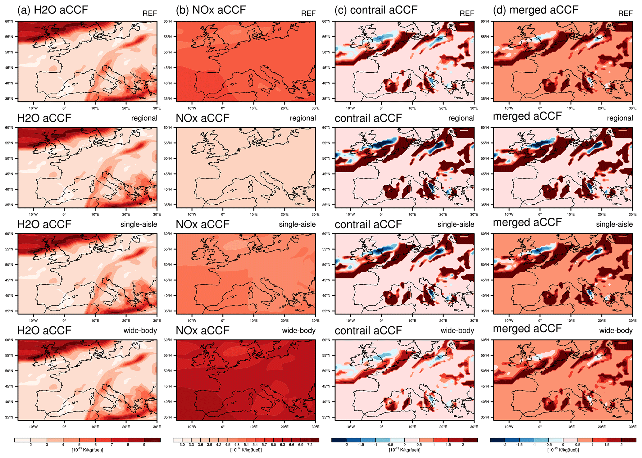
Figure B1Individual aCCFs of water vapor, NOx, and contrail cirrus together with merged aCCFs at a pressure level of 250 hPa over Europe on 15 June 2018 (12:00 UTC) using four different assumptions for the NOx emission index and the specific range values (typical transatlantic fleet mean) (first row): regional aircraft type (second row), single-aisle aircraft type (third row), and wide-body aircraft type (last row). Units are all given in [K kg(fuel)−1]. Note that water vapor aCCFs require no conversion (see Eq. 1).
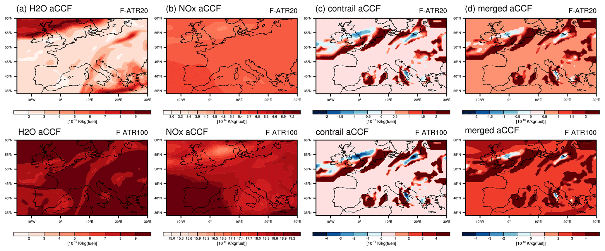
Figure B2Individual aCCFs of water vapor, NOx, and contrail cirrus together with merged aCCFs at a pressure level of 250 hPa over Europe on 15 June 2018 (12:00 UTC) using two different assumptions for the metric: ATR20 and ATR100. Units are all given in [K kg(fuel)−1].
CLIMaCCF is a newly developed open-source Python library. It is developed at https://github.com/dlr-pa/climaccf/ (last access: 5 June 2022) and is available via the DOI (https://doi.org/10.5281/zenodo.6977272, Dietmüller, 2022). It is distributed under the GNU Lesser General Public License (version 3.0). The respective user manual, which includes details on the software and its user configuration, is included as the Supplement to this paper.
The ERA5 data sets used in this study can be freely accessed from the respective repositories after registration. ERA5 data were retrieved from the Copernicus Climate Data Store (https://cds.climate.copernicus.eu/, last access: 8 May 2022, Hersbach et al., 2020) (DOI: https://doi.org/10.24381/cds.bd0915c6, Hersbach et al., 2023).
The supplement related to this article is available online at: https://doi.org/10.5194/gmd-16-4405-2023-supplement.
SD and SM developed the concept of the Python library CLIMaCCF. AS implemented the code to the library (software implementation). AS and HY tested the library. Metric conversion factors were provided by KD, and tabulated aircraft-specific parameters were provided by CW and FL. HY performed the aCCF calculations (used here) with the Python library. SD analyzed the results presented in this paper. SD wrote the paper with text contributions of KD, AS, and FL as well as review from all co-authors. Moreover, all co-authors contributed to the discussion.
At least one of the (co-)authors is a member of the editorial board of Geoscientific Model Development. The peer-review process was guided by an independent editor, and the authors also have no other competing interests to declare.
Publisher's note: Copernicus Publications remains neutral with regard to jurisdictional claims in published maps and institutional affiliations.
High-performance computing simulations with the chemistry–climate model EMAC were performed at the Deutsches Klima-Rechenzentrum (DKRZ), Hamburg.
The current study has been supported by the FlyATM4E project, which has received funding from the SESAR Joint Undertaking (grant agreement no. 891317) under the European Union's Horizon 2020 research and innovation program. Moreover, this project has received funding from the SESAR Joint Undertaking (JU) under grant agreement no. 891467. The JU receives support from the European Union's Horizon 2020 research and innovation program and the SESAR JU members other than the union. Additionally, the ALARM project (SESAR JU under grant agreement no. 891467), coordinated by Manuel Soler (UC3M Madrid), supported this study.
The article processing charges for this open-access publication were covered by the German Aerospace Center (DLR).
This paper was edited by Andrea Stenke and reviewed by Kieran Tait and one anonymous referee.
Appleman, H.: The formation of exhaust condensation trails by jet aircraft, B. Am. Meteorol. Soc., 34, 14–20, 1953. a, b
Bickel, M., Ponater, M., Bock, L., Burkhardt, U., and Reineke, S.: Estimating the effective radiative forcing of contrail cirrus, J. Climate, 33, 1991–2005, 2020. a, b, c
Castino, F., Yin, F., Grewe, V., Soler, M., Simorgh, A., Yamashita, H., Matthes, S., Baumann, S., Dietmüller, S., Linke, F., and Lührs, B.: Seasonal Variability of Aircraft Trajectories reducing NOx-climate Impacts under a Multitude of Weather Patterns, in: 11th SESAR Innovation Days, online, 7–9 December 2021, https://pure.tudelft.nl/ws/portalfiles/portal/113785893/SIDs_2021_paper_81.pdf (last access: 3 March 2022), 2021. a, b
Cess, R., Potter, G., Blanchet, J., Boer, G., Ghan, S., Kiehl, J., Letreut, H., Li, Z., Liang, X., Mitchell, J., Morcrette, J., Randall, D., Riches, M., Roeckner, E., Schlese, U., Slingo, A., Taylor, K., Washington, W., Wetherrald, R., and Yagi, I.: Interpretation of cloud-climate feedback as produced by 14 atmospheric general-circulation models, Science, 245, 513–516, https://doi.org/10.1126/science.245.4917.513, 1989. a
Dahlmann, K., Grewe, V., Frömming, C., and Burkhardt, U.: Can we reliably assess climate mitigation options for air traffic scenarios despite large uncertainties in atmospheric processes?, Transport. Res. D-Tr. E., 46, 40–55, 2016. a, b, c, d
Deuber, O., Sigrun, M., Robert, S., Michael, P., and Ling, L.: A physical metric-based framework for evaluating the climate trade-off between CO2 and contrails – The case of lowering aircraft flight trajectories, Environ. Sci. Policy, 25, 176–185, 2013. a
Dietmüller, S.: dlr-pa/climaccf: Dataset update for GMDD, Zenodo [code], https://doi.org/10.5281/zenodo.6977272, 2022. a, b
DuBois, D. and Paynter, G. C.: “Fuel Flow Method2” for Estimating Aircraft Emissions, SAE Technical Paper 2006-01-1987, SAE Transactions, 1–14, https://doi.org/10.4271/2006-01-1987, 2006. a
FlyATM4E-D1.2: FlyATM4E, Report on expanded aCCFs including robustness and eco-efficiency aspect, D1.2, H2020-SESAR-2019-2, https://flyatm4e.files.wordpress.com/2023/03/flyatm4e_d1.2_00.04.00.pdf (last access: 13 September 2022), 2023. a, b, c, d
Forster, P. D. F., Freckleton, R., and Shine, K.: On aspects of the concept of radiative forcing, Clim. Dynam., 13, 547–560, 1997. a
Frömming, C., Grewe, V., Brinkop, S., Jöckel, P., Haslerud, A. S., Rosanka, S., van Manen, J., and Matthes, S.: Influence of weather situation on non-CO2 aviation climate effects: the REACT4C climate change functions, Atmos. Chem. Phys., 21, 9151–9172, https://doi.org/10.5194/acp-21-9151-2021, 2021. a, b, c, d, e, f, g, h, i
Fuglestvedt, J. S., Shine, K. P., Berntsen, T., Cook, J., Lee, D., Stenke, A., Skeie, R. B., Velders, G., and Waitz, I.: Transport impacts on atmosphere and climate: Metrics, Atmos. Environ., 44, 4648–4677, 2010. a, b, c
Gierens, K., Matthes, S., and Rohs, S.: How well can persistent contrails be predicted?, Aerospace, 7, 169, https://doi.org/10.3390/aerospace7120169, 2020. a
Graver, B. and Rutherford, D.: Transatlantic airline fuel efficiency ranking, 2016, International Council on Clean Transportation, http://www.theicct.org/transpacific-airline-fuel-efficiency-ranking-2016 (last access: 6 May 2022), 2018. a
Grewe, V. and Dahlmann, K.: How ambiguous are climate metrics? And are we prepared to assess and compare the climate impact of new air traffic technologies?, Atmos. Environ., 106, 373–374, 2015. a, b, c, d
Grewe, V. and Stenke, A.: AirClim: an efficient tool for climate evaluation of aircraft technology, Atmos. Chem. Phys., 8, 4621–4639, https://doi.org/10.5194/acp-8-4621-2008, 2008. a
Grewe, V., Frömming, C., Matthes, S., Brinkop, S., Ponater, M., Dietmüller, S., Jöckel, P., Garny, H., Tsati, E., Dahlmann, K., Søvde, O. A., Fuglestvedt, J., Berntsen, T. K., Shine, K. P., Irvine, E. A., Champougny, T., and Hullah, P.: Aircraft routing with minimal climate impact: the REACT4C climate cost function modelling approach (V1.0), Geosci. Model Dev., 7, 175–201, https://doi.org/10.5194/gmd-7-175-2014, 2014. a, b
Grewe, V., Matthes, S., and Dahlmann, K.: The contribution of aviation NOx emissions to climate change: are we ignoring methodological flaws?, Environ. Res. Lett., 14, 121003, https://doi.org/10.1088/1748-9326/ab5dd7, 2019. a
Hansen, J., Sato, M., Ruedy, R., Nazarenko, L., Lacis, A., Schmidt, G., Russell, G., Aleinov, I., Bauer, M., Bauer, S., Bell, N., Cairns, B., Canuto, V., Chandler, M., Cheng, Y., Del Genio, A., Faluvegi, G., Fleming, E. and Friend, A. and Hall, T. and Jackman, C. and Kelley, M. and Kiang, N. and Koch, D. and Lean, J. and Lerner, J. and Lo, K. and Menon, S. and and Miller, R. and Minnis, P. and Novakov, T. and Oinas, V. and Perlwitz, Shindell, D., Stone, P., Sun, S., Tausnev, N., Thresher, D., Wielicki, B., Wong, T., Yao, M., and Zhang, S.: Efficacy of climate forcings, J. Geophys. Res.-Atmos., 110, D18104, https://doi.org/10.1029/2005JD005776, 2005. a, b, c
Hersbach, H., Bell, B., Berrisford, P., Hirahara, S., Horányi, A., Muñoz-Sabater, J., Nicolas, J., Peubey, C., Radu, R., Schepers, D., et al.: The ERA5 global reanalysis, Q. J. Roy. Meteor. Soc., 146, 1999–2049, 2020. a, b
Hersbach, H., Bell, B., Berrisford, P., Biavati, G., Horányi, A., Muñoz Sabater, J., Nicolas, J., Peubey, C., Radu, R., Rozum, I., Schepers, D., Simmons, A., Soci, C., Dee, D., and Thépaut, J.-N.: ERA5 hourly data on pressure levels from 1940 to present, Copernicus Climate Change Service (C3S) Climate Data Store (CDS) [data set], https://doi.org/10.24381/cds.bd0915c6, 2023. a
Irvine, E., Hoskins, B., and Shine, K.: A Lagrangian analysis of ice-supersaturated air over the North Atlantic, J. Geophys. Res.-Atmos., 119, 90–100, 2014. a, b
Irvine, E. A., Hoskins, B. J., Shine, K. P., Lunnon, R. W., and Froemming, C.: Characterizing North Atlantic weather patterns for climate-optimal aircraft routing, Meteorol. Appl., 20, 80–93, 2013. a
Jelinek, F.: The Advanced Emission Model (AEM3)-Validation Report, Ratio, 306, 1–13, https://www.eurocontrol.int/sites/default/files/library/016a_AEM_Validation.pdf (last access: 6 May 2022), 2004. a
Jöckel, P., Tost, H., Pozzer, A., Kunze, M., Kirner, O., Brenninkmeijer, C. A. M., Brinkop, S., Cai, D. S., Dyroff, C., Eckstein, J., Frank, F., Garny, H., Gottschaldt, K.-D., Graf, P., Grewe, V., Kerkweg, A., Kern, B., Matthes, S., Mertens, M., Meul, S., Neumaier, M., Nützel, M., Oberländer-Hayn, S., Ruhnke, R., Runde, T., Sander, R., Scharffe, D., and Zahn, A.: Earth System Chemistry integrated Modelling (ESCiMo) with the Modular Earth Submodel System (MESSy) version 2.51, Geosci. Model Dev., 9, 1153–1200, https://doi.org/10.5194/gmd-9-1153-2016, 2016. a
Joshi, M., Shine, K., Ponater, M., and Stuber, N.: A comparison of climate response to different radiative forcings in the general circulation models: toward an improved metric of climate change, Clim. Dynam., 20, 843–854, https://doi.org/10.1007/s00382-003-0305-9, 2003. a
Kärcher, B.: Formation and radiative forcing of contrail cirrus, Nat. Commun., 9, 1824, https://doi.org/10.1038/s41467-018-04068-0, 2018. a
Lee, D. S., Fahey, D., Skowron, A., Allen, M., Burkhardt, U., Chen, Q., Doherty, S., Freeman, S., Forster, P., Fuglestvedt, J., Gettelman, A., De León, R. R., Lim, L. L., Lund, M. T., Millar, R. J., Owen, B., Penner, J. E., Pitari, G., Prather, M. J., Sausen, R., and Wilcox, L. J.: The contribution of global aviation to anthropogenic climate forcing for 2000 to 2018, Atmos. Environ., 244, 117834, https://doi.org/10.1016/j.atmosenv.2020.117834, 2021. a, b, c, d, e, f, g, h, i, j, k, l, m
Linke, F., Grewe, V., and Gollnick, V.: The implications of intermediate stop operations on aviation emissions and climate, Meteorol. Z., 26, 697–709, 2017. a
Lührs, B., Linke, F., Matthes, S., Grewe, V., and Yin, F.: Climate impact mitigation potential of European air traffic in a weather situation with strong contrail formation, Aerospace, 8, 50, https://doi.org/10.3390/aerospace8020050, 2021. a
Marenco, A., Thouret, V., Nédélec, P., Smit, H., Helten, M., Kley, D., Karcher, F., Simon, P., Law, K., Pyle, J., Poschmann, P., Von Wrede, R., Hume, C., and Cook, T.: Measurement of ozone and water vapor by Airbus in-service aircraft: The MOZAIC airborne program, An overview, J. Geophys. Res.-Atmos., 103, 25631–25642, 1998. a
Matthes, S., Grewe, V., Dahlmann, K., Frömming, C., Irvine, E., Lim, L., Linke, F., Lührs, B., Owen, B., Shine, K., Stromatas, S., Yamashita, H., and Yin, F.: A concept for multi-criteria environmental assessment of aircraft trajectories, Aerospace, 4, 42, https://doi.org/10.3390/aerospace4030042, 2017. a, b
Matthes, S., Lührs, B., Dahlmann, K., Grewe, V., Linke, F., Yin, F., Klingaman, E., and Shine, K. P.: Climate-optimized trajectories and robust mitigation potential: Flying ATM4E, Aerospace, 7, 156, https://doi.org/10.3390/aerospace7110156, 2020. a
Matthes, S., Dahlmann, K., Dietmüller, S., Yamashita, H., Grewe, V., Soler, M., Simorgh, A., González Arriba, D., Linke, F., Lührs, B., Meuser, Maximilian, C. F., and Yin, F.: Concept for identifying robust eco-efficient aircraft trajectories: methodological concept of climate-optimized aircraft trajectories in FlyATM4E, Meteorol. Z., submitted, 2023a. a
Matthes, S., Dietmüller, S., Dahlmann, K., Frömming, C., Yamashita, H., Grewe, V., Yin, F., and Castino, F.: Updated algorithmic climate change functions (aCCF) V1.0A: Evaluation with the climate response model AirClim, Geosci. Model Dev., submitted, 2023b. a, b, c, d, e
Nuic, A. and Mouillet, V.: User Manual for the Base of Aircraft Data (BADA) Family 4, Eurocontrol. ECC Technical/Scientific Report No. 12/11/22‐58, 2012. a
Penner, J. E., Lister, D., Griggs, D. J., Dokken, D. J., and McFarland, M.: Aviation and the global atmosphere: a special report of the Intergovernmental Panel on Climate Change, https://www.ipcc.ch/site/assets/uploads/2018/03/av-en-1.pdf (last access: 22 July 2022), 1999. a
Petzold, A., Neis, P., Rütimann, M., Rohs, S., Berkes, F., Smit, H. G. J., Krämer, M., Spelten, N., Spichtinger, P., Nédélec, P., and Wahner, A.: Ice-supersaturated air masses in the northern mid-latitudes from regular in situ observations by passenger aircraft: vertical distribution, seasonality and tropospheric fingerprint, Atmos. Chem. Phys., 20, 8157–8179, https://doi.org/10.5194/acp-20-8157-2020, 2020. a, b, c, d, e, f
Ponater, M.: Distinctive efficacies of the components contributing to total aviation climate impact, in: 2nd International Conference on Transport, Atmosphere and Climate (TAC-2), 22–25 June 2009, Aachen, Germany and Maastricht, the Netherlands, Deutsches Zentrum für Luft- und Raumfahrt,227–232, ISSN 1434-8454, 2010. a
Ponater, M., Marquart, S., Sausen, R., and Schumann, U.: On contrail climate sensitivity, Geophys. Res. Lett., 32, L10706, https://doi.org/10.1029/2005GL022580, 2005. a, b, c
Ponater, M., Pechtl, S., Sausen, R., Schumann, U., and Hüttig, G.: Potential of the cryoplane technology to reduce aircraft climate impact: A state-of-the-art assessment, Atmos. Environ., 40, 6928–6944, 2006. a, b, c
Pruppacher, H. R., Klett, J. D., and Wang, P. K.: Microphysics of Clouds and Precipitation, Aerosol Sci. Tech., 28, 381–382, https://doi.org/10.1080/02786829808965531, 1998. a
Rao, P., Yin, F., Grewe, V., Yamashita, H., Jöckel, P., Matthes, S., Mertens, M., and Frömming, C.: Case Study for Testing the Validity of NOx-Ozone Algorithmic Climate Change Functions for Optimising Flight Trajectories, Aerospace, 9, 231, https://doi.org/10.3390/aerospace9050231, 2022. a
Rap, A., Forster, P. M., Haywood, J. M., Jones, A., and Boucher, O.: Estimating the climate impact of linear contrails using the UK Met Office climate model, Geophys. Res. Lett., 37, L20703, https://doi.org/10.1029/2010GL045161, 2010. a, b, c
Richardson, T., Forster, P., Smith, C., Maycock, A., Wood, T., Andrews, T., Boucher, O., Faluvegi, G., Fläschner, D., Hodnebrog, Ø., Kasoar, M., Kirkevåg, A., Lamarque, J.‐F., Mülmenstädt, J., Myhre, G., Olivié, D., Portmann, R. W., Samset, B. H., Shawki, D., Shindell, D., Stier, P., Takemura, T., Voulgarakis, A., and Watson‐Parris, D.: Efficacy of climate forcings in PDRMIP models, J. Geophys. Res.-Atmos., 124, 12824–12844, 2019. a
Rieger, V. S., Dietmüller, S., and Ponater, M.: Can feedback analysis be used to uncover the physical origin of climate sensitivity and efficacy differences?, Clim. Dynam., 49, 2831–2844, 2017. a
Simorgh, A., Soler, M., González-Arribas, D., Matthes, S., Grewe, V., Dietmüller, S., Baumann, S., Yamashita, H., Yin, F., Castino, F., Linke, F., Lührs, B., and Meuser, M. M.: A Comprehensive Survey on Recent Climate Optimal Aircraft Trajectory Planning, Aerospace, 9, 146, https://doi.org/10.3390/aerospace9030146, 2022. a, b
Stevenson, D. S., Doherty, R. M., Sanderson, M. G., Collins, W. J., Johnson, C. E., and Derwent, R. G.: Radiative forcing from aircraft NOx emissions: Mechanisms and seasonal dependence, J. Geophys. Res.-Atmos., 109, D17307, https://doi.org/10.1029/2004JD004759, 2004. a, b
Stuber, N., Ponater, M., and Sausen, R.: Why radiative forcing might fail as a predictor of climate change, Clim. Dynam., 24, 497–510, 2005. a
Terrenoire, E., Hauglustaine, D. A., Cohen, Y., Cozic, A., Valorso, R., Lefèvre, F., and Matthes, S.: Impact of present and future aircraft NOx and aerosol emissions on atmospheric composition and associated direct radiative forcing of climate, Atmos. Chem. Phys., 22, 11987–12023, https://doi.org/10.5194/acp-22-11987-2022, 2022. a
van Manen, J. and Grewe, V.: Algorithmic climate change functions for the use in eco-efficient flight planning, Transport. Res. D-Tr. E., 67, 388–405, 2019. a, b, c, d, e, f, g, h, i, j, k
Yamashita, H., Yin, F., Grewe, V., Jöckel, P., Matthes, S., Kern, B., Dahlmann, K., and Frömming, C.: Newly developed aircraft routing options for air traffic simulation in the chemistry–climate model EMAC 2.53: AirTraf 2.0, Geosci. Model Dev., 13, 4869–4890, https://doi.org/10.5194/gmd-13-4869-2020, 2020. a, b
Yamashita, H., Yin, F., Grewe, V., Jöckel, P., Matthes, S., Kern, B., Dahlmann, K., and Frömming, C.: Analysis of aircraft routing strategies for north atlantic flights by using airtraf 2.0, Aerospace, 8, 33, https://doi.org/10.3390/aerospace8020033, 2021. a
Yin, F., Grewe, V., Castino, F., Rao, P., Matthes, S., Dahlmann, K., Dietmüller, S., Frömming, C., Yamashita, H., Peter, P., Klingaman, E., Shine, K. P., Lührs, B., and Linke, F.: Predicting the climate impact of aviation for en-route emissions: the algorithmic climate change function submodel ACCF 1.0 of EMAC 2.53, Geosci. Model Dev., 16, 3313–3334, https://doi.org/10.5194/gmd-16-3313-2023, 2023. a, b, c, d, e, f, g, h, i, j, k, l, m, n, o, p, q, r, s, t, u, v, w
The MOZAIC (Measurement of Ozone, Water Vapour, Carbon Monoxide and Nitrogen Oxides by Airbus In-Service Aircraft) program was designed to collect trace gases by using automatic equipment installed on board five long-range Airbus A340 aircraft operated by European airlines. See Marenco et al. (1998).
- Abstract
- Introduction
- Generation of merged aCCFs
- Technical implementation of individual and merged aCCFs in the Python library CLIMaCCF version 1.0
- Application of CLIMaCCF to ERA5 reanalysis data
- Discussion
- Conclusions
- Appendix A: Mathematical formulation of aCCFs-V1.0
- Appendix B: Additional figures
- Code availability
- Data availability
- Author contributions
- Competing interests
- Disclaimer
- Acknowledgements
- Financial support
- Review statement
- References
- Supplement