the Creative Commons Attribution 4.0 License.
the Creative Commons Attribution 4.0 License.
 | 18 Jan 2023
Implementation and sensitivity analysis of the Dam-Reservoir OPeration model (DROP v1.0) over Spain
Simon Munier
Aaron Boone
Sophie Ricci
The prediction of water resource evolution is considered to be a major challenge for the coming century, particularly in the context of climate change and increasing demographic pressure. Water resources are directly linked to the continental water cycle, and the main processes modulating changes can be represented by global hydrological models. However, anthropogenic impacts on water resources, and in particular the effects of dams-reservoirs on river flows, are still poorly known and generally neglected in coupled land surface–river routing models. This paper presents a parameterized reservoir model, DROP (Dam-Reservoir OPeration), based on Hanasaki's scheme to compute monthly releases given inflows, water demands and the management purpose. With its significantly anthropized river basins, Spain has been chosen as a study case for which simulated outflows and water storage variations are evaluated against in situ observations over the period 1979–2014. Using a default configuration of the reservoir model, results reveal its positive contribution in representing the seasonal cycle of discharge and storage variation, specifically for large-storage capacity irrigation reservoirs. Based on a bounded version of the Nash–Sutcliffe efficiency (NSE) index, called C2M, the overall outflow representation is improved by 43 % in the median. For irrigation reservoirs, the improvement rate reaches 80 %. A comprehensive sensitivity analysis of DROP model parameters was conducted based on the performance of C2M on outflows and volumes using the Sobol method. The results show that the most influential parameter is the threshold coefficient describing the demand-controlled release level. The analysis also reveals the parameters that need to be focused on in order to improve river flow or reservoir water storage modeling by highlighting the difference in the individual effects of the parameters and their interactions depending on whether one focuses on outflows or volume mean seasonal patterns. The results of this generic reservoir scheme show promise for modeling present and future reservoir impacts on the continental hydrology within global land surface–river routing models.
- Article
(6001 KB) - Full-text XML
-
Supplement
(961 KB) - BibTeX
- EndNote


Dams are used to provide essential services to mankind in terms of economic, environmental and social impacts. They provide water supply for domestic, industrial and irrigation needs, enable hydroelectric power generation and river navigation and prevent extreme hydrological events. There are currently more than 58 700 large dams (heights >15 m) worldwide, with an estimated cumulative storage capacity between 7700 and 8300 km3 (Vörösmarty et al., 2003; Downing et al., 2006; Lehner et al., 2011; ICOLD, 2020). When including millions of smaller dams (∼16.7 M larger than 0.01 ha; Lehner et al., 2011), the total global impounded water may even exceed 10 000 km3 (Chao et al., 2008). This means that reservoirs hold more than 4 times the amount of water stored in rivers (the average annual river water storage ranges from approximately 1200 to 2120 km3), and they account for approximately 20 % of average annual river flow to the oceans (40 000–45 500 km3 yr−1) (Baumgartner and Reichel, 1975; Oki and Kanae, 2006; Syed et al., 2010; Lehner et al., 2011). More than 60 % of the world's largest rivers are fragmented by the construction of dams, which account for 90 % of the flow from these river basins (Dynesius and Nilsson, 1994; Revenga et al., 2005; Grill et al., 2015, 2019).
Several studies have demonstrated the significant impact of reservoirs on river flow regimes at not only local scales, but also at larger regional and global scales: reservoirs impact the magnitude of downstream river flows and alter the temporal pattern of river discharge over the continental surface (Haddeland et al., 2006; Hanasaki et al., 2006; Döll et al., 2009; Biemans et al., 2011; Shin et al., 2019; Gutenson et al., 2020). Through surface evaporation and water exchanges with groundwater, lakes and floodplains, reservoirs not only affect the water budget over land, but also throughout the Earth's horological cycle by interacting with the atmosphere and oceans (Pokhrel et al., 2012; Zhao et al., 2012; Wada et al., 2016; Frederikse et al., 2020). There is therefore an increasingly pressing need to integrate reservoir operations in large-scale land surface and global hydrological models (LSMs-GHMs) to overcome the existing biases in continental water cycle and river flow modeling given the number of highly regulated basins.
Models developed to date which represent reservoir releases at a large scale can be categorized as data-driven and process-based approaches. The first category of models is built on the basis of observed release data, water levels and volumes. These methods range from simplified representations of reservoir operation using linear or multilinear regression (e.g., Young, 1967; Raman and Chandramouli, 1996) to very sophisticated models based on machine learning and artificial intelligence techniques, such as neural-network-based methods (e.g., Maier and Dandy, 2000; Razavi and Karamouz, 2007; Ehsani et al., 2016; Coerver et al., 2018). However, this approach requires specific knowledge of the studied reservoirs and requires access to a large amount of observed data. This approach also remains limited in its applicability for future predictions since the generated operational rules are based on historical data and thus do not take into account future potential socioeconomic and predicted climatic changes in the operation of these reservoirs. Process-based approaches, on the other hand, are based on conceptualizing reservoir responses according to its operational purpose by linking release control to physical processes, such as crop growth and the associated water requirements, or to water and energy demands that can be estimated at the global scale. The representation of dam operations is thus achieved without having to explicitly observe the actual release operations performed on each reservoir (Gutenson et al., 2020). The best-known schemes in this category are those developed by Hanasaki et al. (2006) and Haddeland et al. (2006), which are inflow- and demand-based models as presented by Yassin et al. (2019). These two generic models have been implemented in several global hydrological and water management models (e.g., WaterGAP, Döll et al., 2009; VIC, Haddeland et al., 2006; H08, Hanasaki et al., 2008; PCR-GLOBWB, Van Beek et al., 2011).
Of all the studies which have been carried out with these models, very few have been focused on Iberian Peninsula basins, where the prevailing semi-arid climate leads to a greater necessity to store water in large-capacity reservoirs, which leads to larger reservoir effects on rivers (Batalla et al., 2004; López-Moreno et al., 2009; Lorenzo-Lacruz et al., 2010). Spain is, in fact, among the top 10 dam-building countries, with more than 1064 dams (ICOLD, 2020). The study of Grill et al. (2019), which assessed global river connectivity, revealed that the regulation effect of dams is the dominant pressure source in Spain's rivers, where very high degrees of regulation cause an alteration of the natural river flow regime for its five main rivers.
A large number of studies can be found in the literature focusing on the sensitivity analysis of various models, in various science fields, such as machine learning (e.g., Zouhri et al., 2022) or civil engineering (e.g., Zamanian et al., 2021). Pianosi et al. (2016) provided a classification of the sensitivity analysis methods used in environmental sciences and their benefits. A comprehensive sensitivity analysis, as provided by global methods such as Sobol indices, is essential for a precise understanding of a model (Saltelli et al., 2008; Saltelli, 2013). It can help to improve parameter calibration efficiency and avoid overparameterization (e.g., Shin and Jung, 2022; Tang et al., 2007a, b). It is also an efficient tool to better understand the model structure (Saltelli et al., 2008), its uncertainties (e.g., Pheulpin et al., 2022) and the dominant processes under various conditions (e.g., Huang et al., 2021; Zhang et al., 2013). If understanding and quantifying uncertainties is necessary for hydrological modeling, it is also particularly critical to efficiently weight observations and model states in data assimilation techniques (Liu and Gupta, 2007; Abdolghafoorian and Farhadi, 2016). Finally, for a potential extension to the global scale, in which the model parameters cannot be calibrated and validated using observations (that do not exist or are not accessible in most reservoirs of the world), a full understanding of the model sensitivity to the parameters is crucial, especially when models are used as support tools for decision-making (Herrera et al., 2022). A few sensitivity tests on the Hanasaki scheme can be found in the literature (e.g., Hanasaki et al., 2006; Shin et al., 2019), but all of them only focused on one or two parameters supposed to be the most sensitive, which may not be sufficient for a thorough understanding of the impact of parameter uncertainties (Saltelli and Annoni, 2010). To our knowledge, no comprehensive sensitivity analysis has been conducted on this scheme yet.
This study proposes a global and parameterized reservoir model, DROP (Dam-Reservoir OPeration), built on the basis of the generic scheme by Hanasaki et al. (2006), and the aim of the study is to implement it in Spain as a case study to represent reservoir releases and to provide a comprehensive understanding of how uncertainties in each of the model parameters are affecting the overall accuracy of its predictions. In this regard, the study aims to set up a comprehensive sensitivity analysis based on Sobol indices in order to quantify the influence of each parameter and to reveal the types of influence that each of them holds by dissociating individual effects from possible interactions. Further work will focus on implementing this scheme in global hydrological models in order to provide a physical representation of reservoirs on large scales.
This paper is organized as follows: Sect. 2 provides a description of the DROP model and a theoretical outline of the sensitivity analysis method. The study area in Spain, the available observational data, the model setup and the sensitivity analysis implementation are described in Sect. 3. Sections 4–5 illustrate and discuss the model's overall performance and the parameter sensitivity results. Conclusions and perspectives of the study are presented in the last section.
2.1 DROP
The parameterized DROP model has been developed based on the Hanasaki et al. (2006) scheme. The model works at the level of each reservoir individually and is based on the mass balance (as shown below in Eq. 1) of each reservoir to calculate the release at its outlet.
Qin and Qout stand, respectively, for the net inflow to the reservoir and its outflow at the outlet. In fact, the net inflow, Qin, combines different physical processes, as shown in Eq. (2): it includes water inputs from precipitation P, direct runoff Rd representing water flows running off the surrounding ground surface that also feeds the reservoir, and tributary streamflows Qtrib flowing into the reservoir. Evaporation E and groundwater exchange Qgw are also included in Qin.
where Areservoir is the reservoir surface area.
In order to simulate dam releases, Qout, the reservoir model categorizes reservoirs as irrigation and non-irrigation reservoirs, computes the mass balance for each reservoir individually, and calculates releases based on inflow and water demands. A schematic of the DROP model is shown in Fig. 1 with its six parameters (in blue). To give an overview of its overall functioning, the model takes as input inflow and water demands and calculates at a monthly time step dam releases according to the reservoir management purpose and its relative capacity compared to inflow, denoted as c. Operating rules are set following an “operational year”. This type of year has been introduced by Hanasaki et al. (2006), and it differs from hydrological and calendar years. It starts the first month of the water release period and is therefore specific to each reservoir. This specific month, representing the first parameter of the model, will be denoted as mstart in the remaining sections of this article. At the beginning of each operational year, defined by mstart, reservoir storage volume Sinit is compared to the ideal filling value Sideal, defined as a ratio, α, of storage capacity C. Reservoir-simulated releases are impacted by this step as they are retrospectively revised upwards or downwards depending on whether the reservoir has more or less water storage than the ideal rate. Dam monthly releases are then computed following two steps: first, a provisional release is calculated based on water demands and the annual mean inflow. In irrigation reservoirs, two parameters are involved: dmax, setting the control area of the reservoir and thus the water needs to be supplied, and M, defining the minimum release to be provided for environmental requirements. The calculation scheme remains simplistic for other management purposes where releases are set to mean annual inflow. The provisional release is then corrected by incorporating a “demand-controlled release” ratio R, controlled by two parameters cthreshold and b, which accounts for inflow pattern influence in reservoirs with low storage capacities compared to inflow. The DROP model therefore has six parameters, as shown in Fig. 1.

Figure 1Schematic representation of the DROP model showing its six parameters (in blue): mstart defines the start of the reservoir operational year. α sets the ideal filling rate of the reservoir to be reached at each starting month of the year. The remaining four parameters are used in dam release computation: dmax and M, operating only in irrigation reservoirs, set the control area of the reservoir (and therefore irrigation water demands) and the minimum release to be provided, respectively. cthreshold and b, on the other hand, account for inflow pattern influence in reservoirs with low relative storage capacity to inflow (i.e., run-of-river reservoirs).
The operating rules are detailed below. First, at the beginning of each operational year, an annual release coefficient Ky is computed to determine the filling rate of the reservoir. Ky is a ratio between the reservoir storage at the beginning of the year Sfirst,y and the long-term target storage Sideal:
where , α being a nondimensional constant, and C is the total storage capacity of the reservoir. Sideal represents the ideal filling level at the beginning of each year; α was set semi-empirically to 0.85 of the maximum capacity for all reservoirs based on sensitivity tests conducted in Hanasaki et al. (2006). This annual release coefficient is the one used to weight the provisional releases calculated afterwards depending on whether the reservoir has more (Ky>1) or less (Ky<1) water storage than the ideal rate. The underlying aim is to reduce interannual variation in streamflow.
The following steps describe how reservoir releases are computed. The provisional monthly releases, , are set depending on the reservoir's main purpose. The scheme is simplified for a non-irrigation reservoir since it constantly releases the mean annual inflow imean calculated over the whole simulation period (noted “long-term” in the remaining sections of this article):
For an irrigation reservoir, monthly releases are proportional to water demands. They are parameterized here following Shin et al. (2019) as
where dm and dmean,y are, respectively, monthly and annual mean water demands. DPI (demand per inflow) is, as introduced by Shin et al. (2019), the ratio between dmean,y and imean, and M represents the minimum monthly release as a percentage of imean. It is set to 0.5 by Hanasaki et al. (2006) and Döll et al. (2009) and to 0.1 by Biemans et al. (2011) and Shin et al. (2019).
When the DPI is above the set threshold (1−M), water needs are considered to be very high and can only be partially fulfilled by the water stored throughout the coming year. The priority is to first ensure a minimum release, M×(imean), in order to meet the environmental flow requirements. The remaining part of the annual inflow is released throughout the year on a monthly basis following the sub-annual water demand fluctuation curve. Otherwise, when the DPI is below (1−M), the reservoir releases all the monthly water demand that is needed.
In this scheme, only irrigation demand is considered. Since dams provide water for the downstream demand within a certain distance, a maximum distance, dmax, is a parameter to define, for each reservoir, the irrigated grid cells within the river basin to be supplied and thus delimits a “command area” for each reservoir. In contrast to Hanasaki et al. (2006) (where a crop growth model is considered to calculate the irrigation demand), here the distribution of irrigated areas is based on ECOCLIMAP SG (Calvet and Champeaux, 2020; Druel et al., 2022), which is used by the irrigation module in the ISBA LSM (Druel et al., 2022) to compute irrigation demands for 5×5 km-resolution grid cells (see Sect. 3). The irrigation water demands are aggregated within the command area for each reservoir. Unlike the Hanasaki et al. (2006) scheme, the DROP model entirely separates irrigation from non-irrigation reservoirs and only accounts for irrigation water demands for this category of reservoirs. Moreover, industrial and domestic demands are highly uncertain and hardly accessible. In fact, these consumptions are strongly linked to each country's specific political and economical policies, and extensive records are generally not made public. Some global databases, such as the Food and Agriculture Organization of the United Nations (FAO) global information system AQUASTAT (AQUASTAT, 1994), provide estimates of average annual water withdrawals by activity sector and by water resource publicly accessed at the country level. However, such estimates are still limited in terms of temporal and spatial resolution and would consequently add a non-negligible source of error to the model. They are therefore neglected in this study.
In all possible cases, regardless of the reservoir purpose, the water released over the operational year is equivalent to the long-term mean annual inflow.
The release computed so far is provisional. The real monthly release is calculated as follows:
where c is the relative capacity of a reservoir and is defined as the ratio between storage capacity C and the long-term mean annual inflow water volume (). The parameter R, as introduced by Shin et al. (2019) (and also parameterized as β by Horan et al., 2021), is a so-called “demand-controlled release ratio”. It is parameterized in the current study as
where R describes the influence of the inflow regime on release for small storage capacity reservoirs. It varies between 0 and 1 and includes two parameters: cthreshold and the b coefficient. In fact, the smaller the reservoir capacity is compared to inflow, the closer it gets to run-of-river dams where release is close to the natural river flow and thus the influence of the inflow annual pattern. Otherwise, when c is above the threshold (large-capacity dams), then R=1 and the release is fully controlled by water demand. cthreshold and b are set, respectively, as 0.5 and 2 in both Hanasaki et al. (2006) and Biemans et al. (2011). Shin et al. (2019), on the other hand, proposed an analytical formula to compute R, which is reproduced in this study, and set cthreshold and b, respectively, to and 1. The monthly releases are also weighted by the annual coefficient, Ky from Eq. (3), which is calculated at the beginning of the operational year and describes how full the reservoir is relative to the ideal rate. Reservoir releases can therefore be revised upwards or downwards depending on whether the reservoir had more or less water storage than the ideal rate.
The modifications brought to the model from the previous version of Hanasaki et al. (2006) and the Shin et al. (2019) parameterization can be summarized in the following list.
-
The starting month of the operational year, which was calculated in previous versions at the level of each reservoir based on observed inflows and dam releases, is considered in this model version as a parameter, denoted as mstart. This overcomes the challenge faced by the old versions when applying the model in ungauged basins. Within our version, mstart is to be set separately for irrigation and non-irrigation reservoirs.
-
The same applies to dmax, initially set to a constant value depending on the spatial resolution of the river routing model in which the scheme is being implemented in each study. Here, dmax is defined as a parameter to be set for reservoir command area delimitation.
-
dm and dmean,y in Eq. (5) are monthly and annual mean irrigation water demands, respectively. Industrial and domestic water demands are not taken into account, unlike in Hanasaki et al. (2006).
-
M, set to 0.1 in the Biemans et al. (2011) and Shin et al. (2019) schemes and 0.5 in Hanasaki et al. (2006), is considered as a parameter in this version, keeping the same notation used in Shin et al. (2019).
-
A more explicit parameterization of the demand-controlled release ratio R is provided here compared to what is proposed in Shin et al. (2019). The generalized formulation of R in Eq. (7) highlights the last two parameters of the present model version. This enables one to distinguish the dual role of cthreshold in Eq. (6) from that of the coefficient b, which only describes the transition made between a demand-controlled reservoir and an input-controlled reservoir. Hanasaki et al. (2006) and Shin et al. (2019) have set (cthreshold, b) to (0.5,2) and (,1), respectively.
A description of the reservoir model parameters is given in Table 1.

The reservoir volume is derived at each time step from the water balance. Boundary conditions are defined considering two possible scenarios: (i) if the reservoir is full, the excess water is spilled. (ii) When reservoir storage falls below 10 % of the capacity, the reservoir reaches the dead storage zone and water release is prevented.
In order to run the model, reservoir characteristics, such as the storage capacity and main purpose, are needed. The model also requires continuous time series of inflow and water demands to compute releases. In the current study, all of the modeled reservoirs are located in Spain, where the physical characteristics, in situ observations of natural and anthropized flows, and storage volumes are publicly available. Section 3 describes the global and local datasets used herein.
2.2 Sensitivity analysis: Sobol's method
The Sobol sensitivity analysis method (Sobol, 1993) has been widely used in hydrological models in order to identify the parameters that contribute the most to the model output uncertainty. It is a global variance-based approach where, for a chosen variable of interest Y, the total variance is decomposed into fractions attributed to each individual input as well as the interactions between them. If Y=f(X) is a goodness-of-fit metric of the model with X representing the set of parameters of size p, the total variance of Y, D(Y), is decomposed as follows (Zhang et al., 2013):
where Di is the amount of variance due to a parameter Xi alone, Dij is the amount of variance arising from the interaction between the parameters Xi and Xj, and so on. Equation (8) is known as Hoeffding decomposition (Hoeffding, 1992).
The sensitivity indices, called Sobol indices, are computed as ratios between the component variances and total variance in order to measure the contribution of each single parameter and each parameter interaction. The first-order Sobol index, S1, captures the sensitivity of Y to each input parameter Xi taken alone. The second-, S2, and higher-order indices describe the contribution of the multiple interactions between parameters. A model with p parameters requires 2p−1 indices to be evaluated, which rapidly becomes computationally challenging for high values of p. The total-order index, ST, measures the full influence of a parameter by including all of the variance caused by its interactions with the rest of the parameters, all orders included. The first-, second- and total-order Sobol sensitivity measure formulas are
where D∼i is the amount of variance due to all of the parameters except for Xi.
Model parameter sampling and Sobol index estimation are performed here using the open-source Python library SALib (Herman, 2017). The parameter samples are generated following quasi-random sequences (Saltelli, 2002) in order to scatter the sample points as uniformly as possible over the parameter space. Following the theorem, the different orders of Sobol indices are estimated from a total number of model runs of , where N and d are, respectively, the sample size and the number of parameters. The package also provides confidence intervals of the index estimates at the 95 % confidence level.
3.1 Spain river basins description
Spain has an estimated area of 505 983 km2 (INE, 2022), representing more than 85 % of the Iberian Peninsula (estimated area 583 254 km2, Lorenzo-Lacruz et al., 2012). It has river basins with sizes ranging from a few square kilometers to more than 80 000 km2 (i.e., the Ebro basin). The five largest river basins are the Ebro, flowing into the Mediterranean Sea, and the Duero, Tajo, Guardiana and Guadalquivir, flowing into the Atlantic Ocean. They also represent the river basins where the natural river flow pattern is the most significantly altered in the country, with high degrees of regulation resulting from extensive reservoir construction. These different rivers have a Mediterranean hydrological pattern, which is characterized by high flows during the wet season (i.e., fall and winter) and low flows during its dry season (i.e., late spring, summer). This seasonality explains the strong anthropization of the Spanish hydrographic basins and, in particular, the construction of more than 1200 dams mainly in the second half of the 20th century. They are essential for retaining enough water to meet irrigation and domestic water demands as well as for hydropower production, which represents ∼13 % of Spanish electricity generation (IEA, 2022, in 2020,).
3.2 Dataset
The data series required as inputs to the model and the ones used to validate the outputs are taken from the Spain database. Reservoir characteristics are taken from the global GRanD database. Irrigation demands are simulated by the ISBA irrigation module. The needed input data are detailed below.
-
Local (Spain) database. In situ observations of natural and anthropized flow and volume data are made publicly available by the Center for Hydrographic Studies of Spain (CEDEX, Ministry of Public Works and Ministry for Ecological Transition, Spain). The national database includes the location and daily time series of discharge for 1119 gauge stations and outflows from 347 reservoirs over the period 1900–2014.
-
The Global Reservoir and Dam (GRanD) database, from which the general characteristics of dams are taken (Lehner et al., 2011). Version 1.3 published in 2019 includes 7320 reservoirs and provides the geographical locations of dams as well as attribute information such as the construction year, maximum storage capacity, surface area and set of purposes of reservoirs; 263 of the reservoirs listed in GRanD are located in Spain. Most of them were built from 1955 to 2000, reaching a total storage capacity of 56 480 hm3 in 2016, which exceeds the mean annual streamflow of the eight major rivers of the Iberian Peninsula (55 850 hm3 yr−1) (Lorenzo-Lacruz et al., 2012). Irrigation and hydroelectricity are the most identified purposes of more than half the reservoirs, and water supply comes third. In this paper, all management purposes different from irrigation are grouped in the “other purposes” category.
-
Simulated irrigation demands. The irrigation water demands are simulated by the new irrigation scheme implemented in the ISBA LSM (Druel et al., 2022). It uses the ECOCLIMAP-SG land cover classification to identify the areas within the grid cell that can be irrigated. The three main parameters are set in the model to control, respectively, the irrigation triggering (when the plant reaches the wilting point), the period of crop growth where irrigation is possible (between emergence and harvest) and the amount of water used for irrigation. In the default configuration, a predefined amount of water of 30 mm is set for each irrigation and a 7 d minimum return period is fixed between two irrigation operations. These parameters can be user-defined for each vegetation type and in each grid cell. To generate irrigation demands over Spain, we used the 5 km resolution SAFRAN-based meteorological datasets for that country (Quintana-Seguí et al., 2017) that were available over the period 1979–2014 to force the ISBA land surface model. Set to the default configuration, the irrigation module within the LSM computed daily irrigation demands for each grid cell over that time period. At the input of the reservoir model, dmax is set beforehand and delimits for each reservoir a command area made up of a selection of grid cells within the same basin at a lower altitude. The equivalent amount of irrigation water requested from a reservoir in a given month corresponds to the aggregated daily irrigation demands of all crop types within the retained grid cells.
3.3 Model setup: pre-processing steps
3.3.1 Cross-referencing global and local datasets
Out of the 263 reservoirs listed in GRanD, only 216 were kept after cross-referencing the two databases and for which both the characteristics and time series of release and volume could be identified. In fact, two reservoirs were doubly identified in GRanD v1.3 (the IDs were 2882 and 2844) because they were rebuilt and/or renamed; their most recent characteristics are those retained. The 45 remaining reservoirs, located mainly in the northwest and south of Spain, were not identified in the Spanish database since they were built after 2014.
The maximum storage capacity of the chosen reservoirs goes from 9.5 (the San Lorenzo Mongay dam, located on the Segre River in the Ebro basin) to 3200 hm3 (the La Serena dam on the Zujar River in the Gardiana basin), with a mean of 236 hm3 and a standard deviation of 441 hm3. Using the latitude and longitude information, the chosen reservoirs were located on the new ∘-resolution river network derived from the CTRIP river routing model (Munier and Decharme, 2022). Dam locations were adjusted so as to have comparable drainage surfaces between those given by the GRanD database and those estimated by CTRIP.
An initial analysis conducted on observed river flows upstream and downstream of the reservoirs has identified a common seasonal behavior among those with irrigation, which is that the peak dam release is shifted in time from the natural inflow. This is due to the typical operating mode of these reservoirs, which are designed to retain water arriving upstream during winter (wet season) and release it during summer (dry season) to meet irrigation needs.
3.3.2 Reconstructing inflow
The reservoir scheme requires reservoir net inflows and water demands as inputs to estimate volume variations and outflows. In existing studies, water demands are estimated and net inflows are either modeled by a river routing scheme or estimated from gauge observations in rivers and tributaries upstream the reservoir. Reservoir abstraction is also sometimes accounted for in the reservoir water balance. However, some processes are usually neglected, such as precipitation interception, direct runoff, evaporation or groundwater exchanges. This introduces a bias into the water budget and consequently increases the model uncertainties, especially when inflows are derived from land surface and river routing models (see, e.g., Vanderkelen et al., 2022). In this study, the water balance (Eq. 2) is used in a first step to derive the result of all these components (net inflow) from observations of reservoir volume and outflow, as described below. The advantage compared to previous studies is that it removes the uncertainties related to each of these components, enabling the analysis of the model uncertainties themselves and the capacity of the model to reproduce the reservoir behavior alone, without additional uncertainties or potential compensations between the components of the water budget and the model parameters.
Note that, in a future work, the DROP model aims to be coupled to a series of models that can represent these different processes. In the ISBA-CTRIP land surface–river routing model, for example (Decharme et al., 2019), evaporation is computed by FLake, a module representing energy balance in lakes (Le Moigne et al., 2016), direct runoff is derived from the ISBA land surface model, and inflows from tributaries as well as groundwater exchanges are computed by the CTRIP river routing model (Munier and Decharme, 2022).
For each of the selected reservoirs, the longest continuous common periods of daily observed outflows and volumes were first determined. At this stage, only reservoirs with more than 3-year time series were retained, which leaves 215 reservoirs to be simulated. The net inflows were then derived from outflows and volume variations at the daily scale (Eq. 1). The computed net inflows were then corrected by removing outliers in two steps: first, all peak flows were selected when their maximum value exceeded 5 times the long-term mean. Among the peak values, outliers are then identified when the relative difference of slopes before and after peak flow is less than 10 %. Both thresholds were set empirically. This step differentiates the outliers from the hydraulic behavior of a river in flood recession periods. The outlier is replaced by a linearly interpolated value. The length of the corrected time series goes from 3.5 to 34 years with a median of 23 years. The main purposes, simulation period lengths and relative capacities of the 215 reservoirs simulated are shown in Fig. 2.
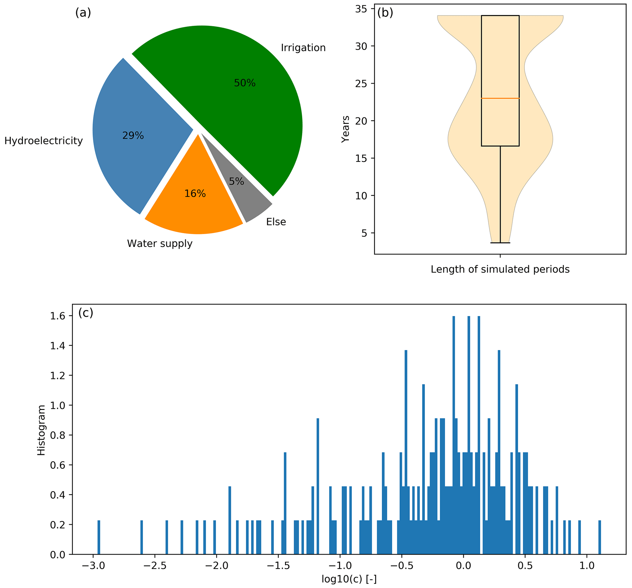
Figure 2Main characteristics of the chosen reservoirs. (a) Classification of their main purpose, (b) distribution of simulation period lengths, and (c) histogram showing decimal log values of their relative capacity.
We note a good distribution of management purposes and relative inflow capacities in the final selected reservoirs. Overall, half the reservoirs are primarily used for irrigation, which is mainly due to the semi-arid climate of the Iberian Peninsula and the high needs of irrigation in the country. The rest of the reservoirs are allocated to hydropower generation, water supply and different other purposes with respective percentages of 29 %, 16 % and 5 % and are grouped in the non-irrigation reservoir category.
3.4 Sensitivity analysis implementation
A sensitivity analysis with respect to the six parameters was conducted on the performance of a Nash–Sutcliffe efficiency (NSE, Nash and Sutcliffe, 1970) bounded version, called C2M (Mathevet et al., 2006), on outflows using the Sobol method. In fact, the NSE values in some reservoirs were highly negative for some simulations, and thus this metric was not suitable for a variance-based sensitivity analysis method like Sobol's. C2M is used instead as it is a normalized version of NSE that varies between −1 and 1 and where all negative values are bounded between 0 and −1. Parameter default values, bounds and distributions are listed in Table 2. The parameter distributions were all considered uniform except for relative capacity, for which the distribution is logarithmic to align with the observed pattern on the modeled reservoirs (Fig. 2).
Table 2Summary of the DROP model parameter default values and feasible ranges for the sensitivity analysis.
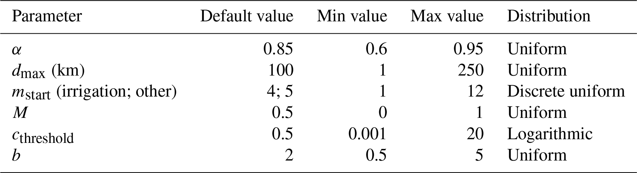
The default values for α, M, cthreshold and b are those considered in Hanasaki et al. (2006). α-selected bounds cover a realistic range of ideal reservoir filling rates. The distribution and bound values of the cthreshold parameter are drawn from the relative capacity distribution of the 215 modeled reservoirs (Fig. 2). The b lower limit is 0.5, below which the shift to the demand-controlled state of a reservoir becomes too abrupt once c exceeds cthreshold. The upper limit considered for b is 5, beyond which the transition curve between the behavior of a low relative capacity reservoir and a high relative capacity one becomes unchanged, following the sensitivity test run conducted on this parameter. For dmax, both the default value and the lower and upper limits were set to be consistent with the sizes of Spanish river basins. The operational year starting month, mstart, is set to April for irrigation reservoirs in order to match the beginning of the crop irrigation season considered in the irrigation model. For other reservoirs, mstart is chosen empirically to be May as the default value based on the observed filling curves of the reservoirs, which tend to be at the maximum filling level near May.
The sensitivity analysis was performed on each of the 215 reservoirs separately, distinguishing between irrigation and non-irrigation reservoirs since the number of parameters involved depends on the main purpose of the reservoir (six and four, respectively, as dmax and M are only considered in irrigation reservoirs).
Using Saltelli's quasi-random sampling method (Saltelli et al., 2010), a sample size of 4096 was used for this analysis in each category, resulting in and model runs for each of the 107 irrigation and 108 non-irrigation reservoirs, respectively. By comparing with smaller sample sizes, the confidence intervals estimated by SALib show that the Sobol indices converged and that the chosen sample size is sufficient to reliably represent the results.
This section presents the main results of this study. First, simulation results of the reservoir releases using the default configuration of the model are displayed. Then, a sensitivity analysis of the model parameters is presented.
4.1 Reproducing the flow seasonal shift in irrigation reservoirs
Using the default parameterization with the parameters listed in Table 2, an operating rule is determined for each of the 215 reservoirs, and both outflows and water storage variations are simulated through complete operational years within the overall period 1979–2014. Figure 3 shows the C2M values at reservoir outlets by evaluating the simulated monthly outflow time series against in situ observations. Panel a shows the results obtained using a reference simulation where rivers are considered in their natural state (Qout=Qin). Panel b shows the C2M improvement rate when considering the DROP model.
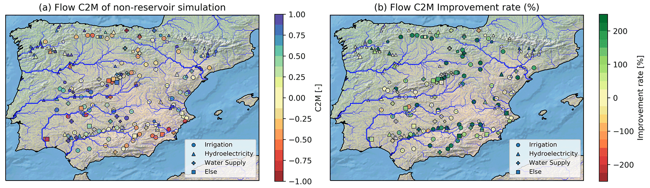
Figure 3Results of the DROP model contribution (default configuration) in river flow modeling at reservoir outlets: (a) C2M performance metrics of non-reservoir simulation (reference simulation where Qout=Qin) and (b) C2M improvement rates by integrating the reservoir model. Symbols represent the different reservoir management purposes. They come in two different sizes: larger if c≥0.5 and smaller if c<0.5.
Overall, with DROP, the river flow representation is clearly improved at nearly all the reservoirs' locations. The median C2M index for flows is 0.52, which corresponds to a 43 % improved flow representation when compared to natural river representation. For storage volume representation, the mean correlation is 0.53 with a standard deviation of 0.3. Half of the reservoirs have a correlation greater than 0.63 between observed and simulated storage volumes.
The results reveal the model's positive contribution in representing the seasonal cycle of river flow, specifically for irrigation large-storage capacity reservoirs, as the model reproduces the seasonal shift between inflows and outflows caused by irrigation management rules with reasonable accuracy. For these reservoirs, the correlation between simulated and observed discharge increases from 0.49 (reference simulation) to 0.75 in the median. Regarding storage volumes, correlation reaches 0.74 in the median. As an example, the Gonzalez Lacasa reservoir located in the Ebro basin shows typical results in Fig. 4. In fact, this irrigation reservoir stores incoming water during winter/early spring, which explains a lower outflow than inflow (in blue and orange, respectively, for observed discharges, panels (a) and (b) in Fig. 4) between October and March and releases the water in summer when there is insufficient water to supply all crops' irrigation needs. The period of release, from April to September in this case (shown in the annual cycle, Fig. 4c), corresponds to the crop-growing period and therefore to high irrigation water needs. As a result, the discharge seasonal curve is shifted and the maximum monthly discharge, in this example, is reached in July instead of April. This management scheme is well reproduced by the DROP model, as the simulated outflows (shown in red) align well with the observations (in blue), and consequently so do the volume variations.
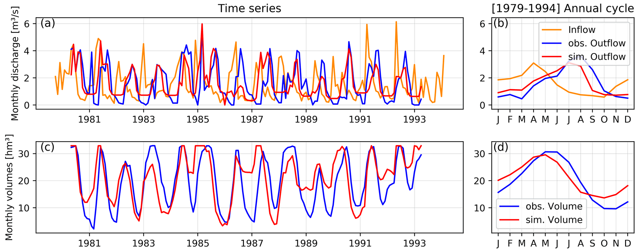
Figure 4Simulation results for the Gonzalez Lacasa irrigation reservoir within the Ebro River basin over the period [1979–1994]. The monthly time series of dam releases and storage volumes are shown in panels (a) and (c), respectively (observations are indicated in blue and simulations in red). Their corresponding mean annual cycles are shown in panels (b) and (d), respectively.
The improvement of the C2M distribution for each category of dams, in terms of main purpose and relative capacity, is shown in Fig. 5. Note that, for irrigation reservoirs, the improvement rate reaches 80 % in terms of the median and 123 % for those considered of high relative capacity (here c≥0.5) and which are fully demand-controlled. The flow improvement rates for the rest of the high relative capacity reservoirs are dispersed but remain positive at the median despite the simplistic approach of DROP. For low relative capacity reservoirs (here c<0.5), and independent of the management purpose, the model's contribution is almost null since the reservoirs are considered “run-of-river” and the influence of the inflow regime is predominant.
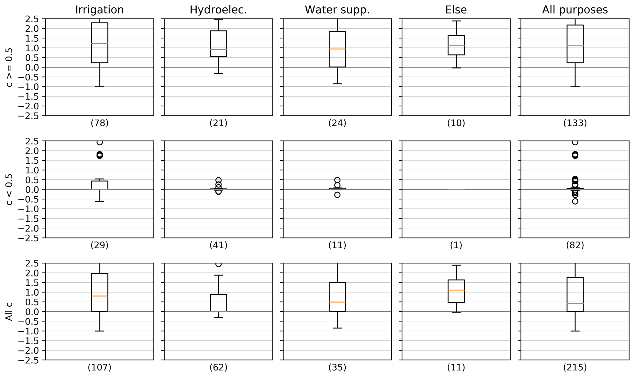
Figure 5Distribution of river flow, C2M, improvement rates with the DROP model based on their main purpose (columns) and relative capacity (rows). The x-axis labels show the number of reservoirs in each category, and the y axis shows C2M improvement rates.
4.2 Results of the sensitivity analysis
The distributions of first-order Sobol indices for each parameter calculated at each of the 107 irrigation and 108 non-irrigation reservoirs are shown in Fig. 6 with a box plot. Overall, it emerges from Fig. 6 that the most influential parameter is cthreshold. In fact, based on the definition of S1, ∼48 % of the total variance in C2M is attributed to cthreshold alone within irrigation reservoirs. In non-irrigation reservoirs, this parameter accounts for ∼74 % of C2M variance. The M parameter is ranked second in irrigation reservoirs and accounts for 15 % alone in the median of all of the variance, followed by dmax with an S1 index of 0.03. The parameter controlling the month for which the operational year starts, mstart, alone has very little influence on the overall outflow C2M variance, although the effect is slightly more noticeable in the non-irrigation reservoirs. α and b are considered the least influential parameters for most reservoirs.

Figure 6Distribution of first (S1)-order Sobol indices in the modeled reservoirs for each parameter: (a) in irrigation and (b) in non-irrigation reservoirs.
To better illustrate how each parameter individually affects the model outputs, the Gonzalez Lacasa reservoir (GRanD ID 2699; c=0.65) is set as an example. Given the sensitivity analysis results, a screening step is added on cthreshold, M and α separately and the rest of the parameters are set to their default values. The means of monthly outflows over the simulation period (1979–1994) are shown in Fig. 7.
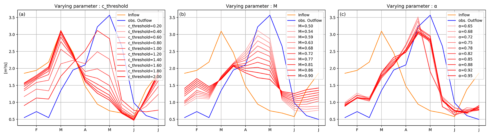
Figure 7Example of seasonal pattern sensitivity of Gonzalez Lacasa reservoir outflow to three of the DROP model parameters: (a) cthreshold, (b) M and (c) α. The remaining parameters were at their default values (see Table 2).
Regarding the first parameter and for values of cthreshold below the relative capacity of the reservoir (lower than 0.65 for the Gonzalez Lacasa case), the reservoir is considered with high storage capacity, and so monthly releases are completely driven by demand, resulting in a seasonal shift between inflow and outflow and a peak of discharge in July in order to meet the irrigation needs. Conversely, when the cthreshold is higher, the dam is considered to have a low storage capacity, which reduces the buffering effect and increasingly aligns the simulated release curve (in red) with the seasonal trend cycle of inflow (in orange), as shown in Fig. 7a. The buffer role of the reservoir is therefore conditioned by the value of the cthreshold.
The influence of M on the minimum release is shown in Fig. 7b. The higher the value of M, the greater the part of mean inflow set as minimum release and the lower the remaining part of water dedicated to meeting irrigation needs during peak demand. Since the Gonzalez Lacasa reservoir is considered to have a relatively large storage capacity (with cthreshold=0.5 as the default value) among the considered reservoirs, the outflow will still follow the seasonal curve of water demand, but M will influence the release peak by extending or flattening the outflow curve to maintain a minimum release level required through the year. For run-of-river dams, M is irrelevant since the release follows the monthly inflow. dmax also controls the variation of outflows over the year in the same way, but only when the DPI ratio is low. Its impact remains limited beyond the (1−M) threshold, as the release curve is fixed to maintain the required minimum outflow.
The parameter α, on the other hand, does not affect the long-term mean pattern of release. In fact, α only operates on outflows on an inter-annual basis, through Ky, to offset the excess or shortage of stored water from one year to the other, especially when the critical filling zones are reached (reservoir in a dead storage zone or overflowing), in order to bring the reservoir water state to the ideal filling curve over the long term (Fig. 7c). The same behavior is noted for mstart, which is not shown in Fig. 7.
The cthreshold, α and mstart parameters have the same effect on non-irrigation reservoirs. The influence of each of the three parameters on [1979–2013] monthly mean outflows from the “Alcantara II” reservoir (GRanD ID 2800) in the Tagus River basin, which has a relative capacity of 0.6 and is mainly used for electricity generation, is shown in Fig. 8. For this specific reservoir, the simulated period includes several wet years, and there were periods when water flowed over the spillways during winter, which explains the alignment of the outflow with the inflow during this season.

Figure 8An example of the seasonal pattern sensitivity of the Alcantara II hydroelectricity reservoir outflow to three of the DROP model parameters: (a) cthreshold, (b) α and (c) mstart. The remaining parameters were set at default values (see Table 2).
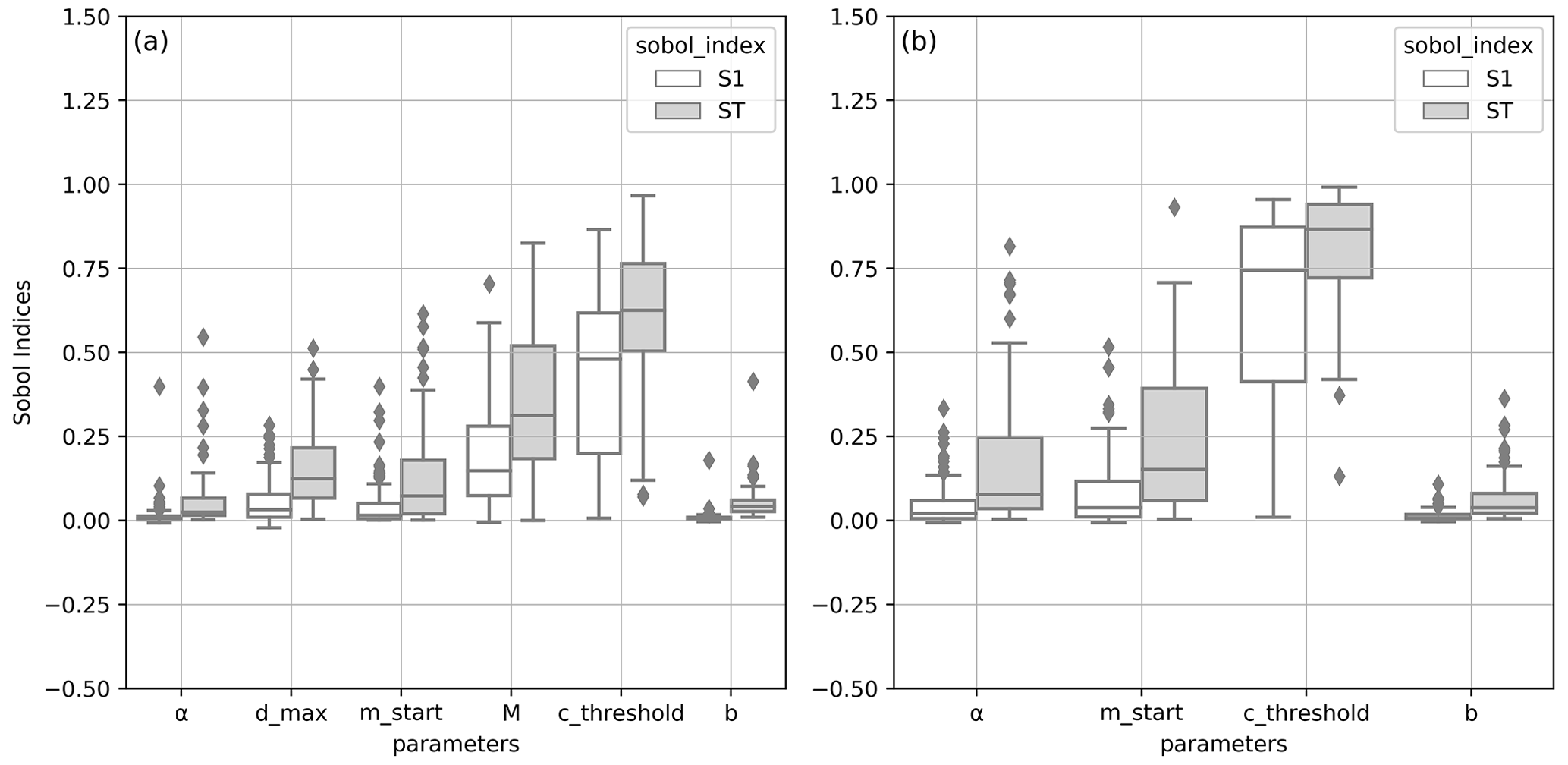
Figure 9Distribution of first (S1)- and total (ST)-order Sobol indices in the modeled reservoirs for each parameter: (a) in irrigation and (b) in non-irrigation reservoirs.
The distributions of total sensitivity indices ST (in grey), alongside S1 (in white), of each parameter are shown in Fig. 9. A significant gap is observed between the first- and total-order index distributions. This confirms the non-negligible effect of the parameters' interactions on the output variance involving mainly cthreshold. In the median, based on the ST definition, ∼62 % of C2M variance in irrigation reservoirs and ∼87 % in non-irrigation reservoirs are attributed exclusively to cthreshold and its interactions with other parameters: it is indeed the most important parameter of the DROP model. α and b, on the other hand, were in the median low values, which makes them the least important parameters.
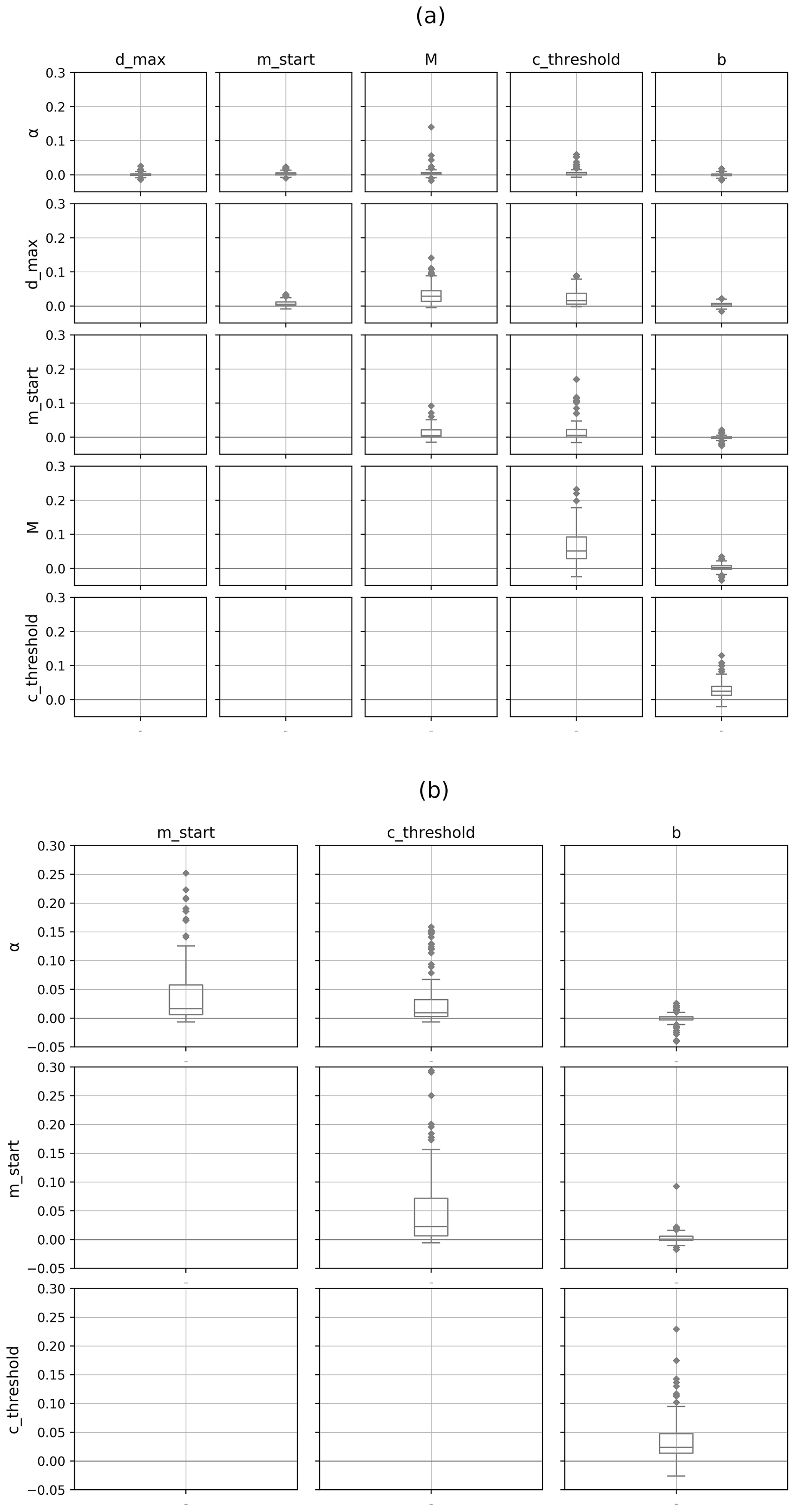
Figure 10Distribution of second-order Sobol indices (S2) in the modeled reservoirs for each pair of parameters: (a) in irrigation and (b) in non-irrigation reservoirs.
The distributions of second-order Sobol indices for each parameter couple for the irrigation and non-irrigation reservoirs considered separately are shown in Fig. 10. The results reveal that the parameter with the most interactions overall with other parameters is cthreshold. This is mainly due to its position at the end of the model chain, where provisional releases are corrected. For the rest of the parameters, the interaction between mstart and α is more marked in non-irrigation reservoirs since the scheme is simplistic and the outflow depends mainly on the Ky annual coefficient that is driven by both mstart and α. In irrigation reservoirs, the coefficients dmax and M interact because they control irrigation water demand and the reservoir water storage allocated to it. As they are both involved in the reservoir water balance, they jointly control the outflow. The b coefficient meanwhile interacts only with cthreshold when computing the demand-controlled release ratio R calculation. The total influence of b, mostly resulting from the interaction with cthreshold, is only seen in reservoirs with low relative capacities.
Since c is a defining characteristic of each reservoir and is involved in the outflow computation, the first- and total-order Sobol indices were rearranged according to their reservoir-correspondent c values, here grouped into six ranges to simplify the presentation of the results to better identify the impact on parameter ordering and interactions (Fig. 11).
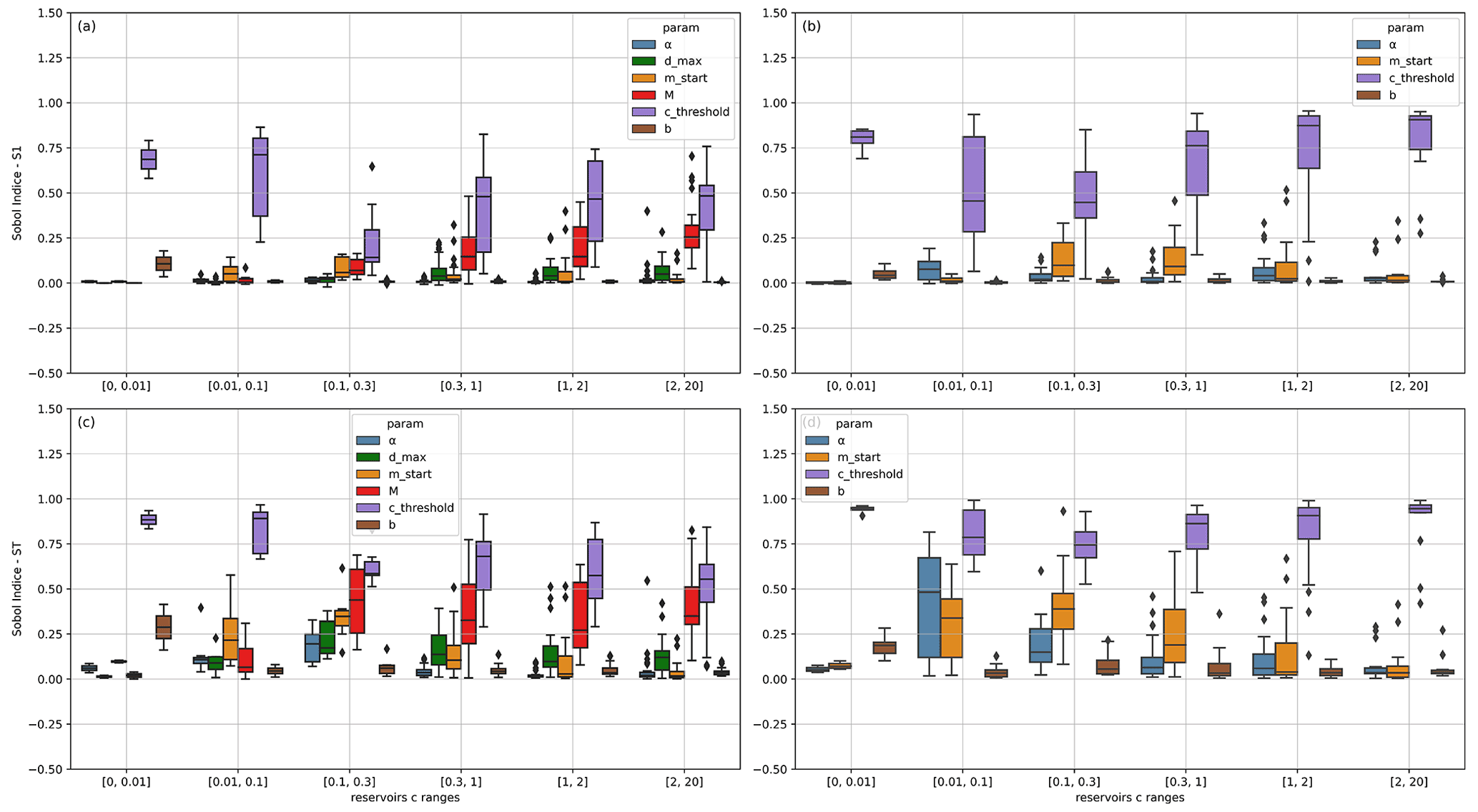
Figure 11Distribution of first- (“S1”) and total-order (“ST”) Sobol indices of parameters according to relative capacity: (a, c) in irrigation and (b, d) in non-irrigation reservoirs.
For low values of c (less than 0.01), cthreshold is the only relevant parameter. The total influence of b, on the other hand, is mostly related to its interaction with cthreshold. The remaining parameters are negligible since their first-order Sobol indices are almost zero and the total order is very low. For reservoirs with a medium storage capacity (), a significant part of total variance is due to parameter interactions, apart from b, as all Sobol indices increase significantly from first to total order. This is even more noticeable when . Above a relative capacity of 0.3, the M parameter in irrigation reservoirs gains in importance and increases interactions with the cthreshold as c is bigger. For non-irrigation reservoirs of the same category, cthreshold takes on more importance as the storage capacity increases (less spreading and very high S1). The remaining parameters lose relative importance. For the very high relative capacity values, α and mstart are almost irrelevant, regardless of the operating objective. Finally, for nearly all reservoirs combined (except those with very small values of c), the b coefficient has almost no influence and can therefore be set to a nominal value.
When using Sobol indices, the representation of model output uncertainty is limited to the variance only, which is not fully representative of all the statistical characteristics (or moments) of the C2M distribution. Using the distribution function instead provides a complete description of uncertainty in the model output. Here, we evaluate the sensitivity of parameters by assessing their influence on the entire C2M distribution without reference to a specific moment of the output (Chun et al., 2000; Borgonovo, 2007, moment-independent methods). This method is used as a validation step for the overall conclusions found with the variance-based Sobol method. The deviation of the C2M distribution function caused by two different parameters cthreshold and α over the irrigation reservoirs is shown in Fig. 12. Here, the same samples generated for Sobol's index calculation were used. First, the unconditional probability distribution function (PDF) of the model output C2M is obtained when all input parameters are randomly sampled from their distributions. Then, for each input parameter, conditional PDFs of C2M are computed following different value ranges from the total parameter distribution: here, five ranges are considered. The importance of each parameter is proportional to the magnitude of the conditional PDF deviation from the unconditional one.
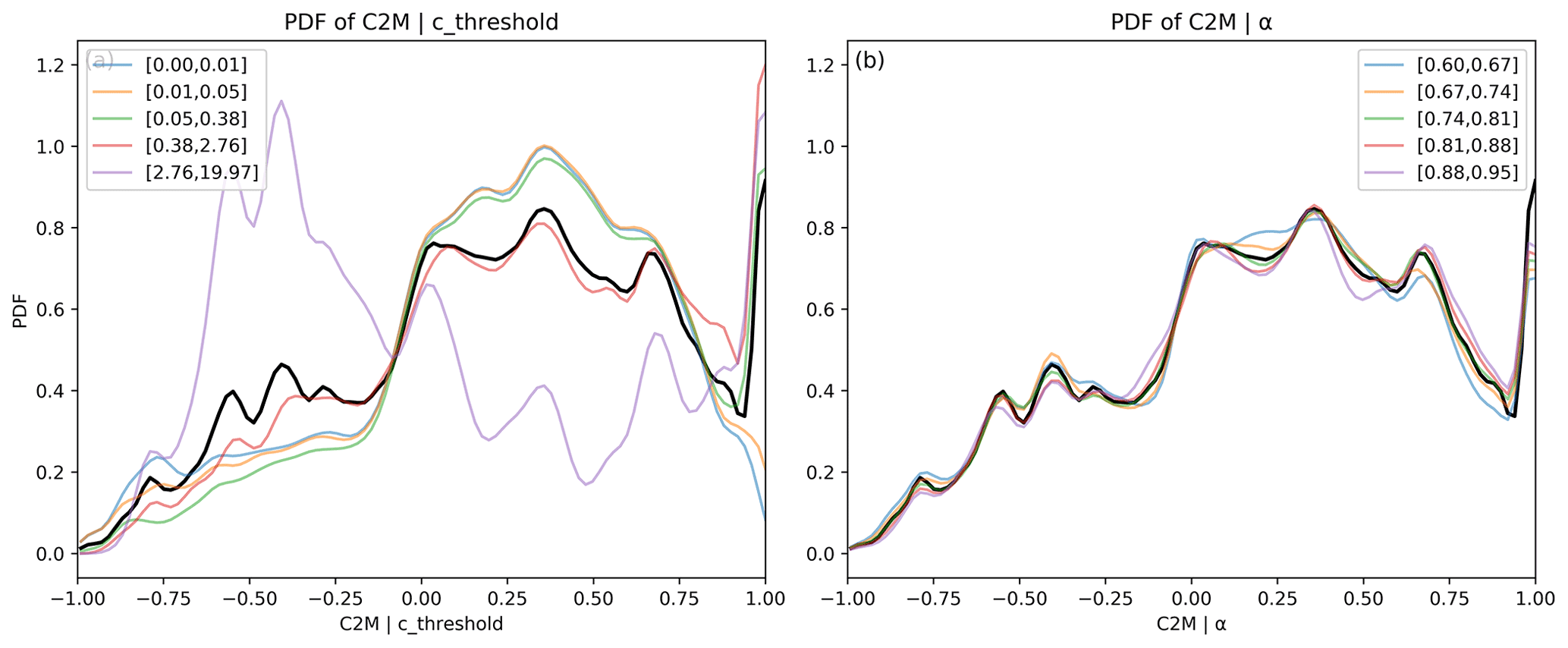
Figure 12Shifts in C2M' probability distribution function (PDF) depending on cthreshold (a) and α (b) range values, within irrigation reservoirs. The unconditional PDFs of the DROP model output C2M, obtained when all input parameters are randomly sampled, are displayed in black. The conditional PDFs are shown in color depending on the parameter value range.
The large dispersion of the conditional PDFs (colored) shows the strong impact of cthreshold in the model outlet in Fig. 12a. All PDFs are nearly aligned for α, and thus the value of this parameter has very little significance for C2M distribution. Moment-independent sensitivity indicators like “Kolmogorov”, “Kuiper” and “Delta” (Borgonovo and Plischke, 2016) were used to measure the deviation from the unconditional PDF, and the results were consistent with the conclusions made with the Sobol index. It is also noted that DROP tends to have very poor performance scores for high values of cthreshold (above 2.76) where all the reservoirs are considered run-of-river and the release would be close to the lines alignments with inflow as shown in Fig. 12. This figure indirectly demonstrates the reservoir model contribution in terms of improving river flow representation in anthropized basins where the magnitude and seasonal flow dynamics are significantly altered by large storage capacity reservoirs, especially those for irrigation purposes.
5.1 Limits of the DROP model scheme
The DROP model outputs are affected by several uncertainties linked to the model inputs and the algorithm. The parameterized model is based on a generic scheme of reservoir operation, which inevitably implies a simplification in terms of water release. Concerning the representation of operational purposes, the algorithm fails to differentiate between other purposes than irrigation and considers that a constant release is expected by the rest of the reservoirs. In addition, only the main objective of the reservoir is represented, and the releases of the multi-purpose reservoirs are not entirely represented since their management rules are more complex to describe. This explains the poor performance of the model at the level of reservoirs that are used for irrigation, though it is not their main objective: DROP is very simplistic for the rest of its possible purposes, so that the seasonal shift in water discharge is not always well reproduced. This is the case of the reservoir “Los Bermejales”, for example, a multi-purpose reservoir located in the basin of the Guadalquivir River, southern Spain, which is mainly used for water supply, but it is also used to meet irrigation water demands (Fig. 13).
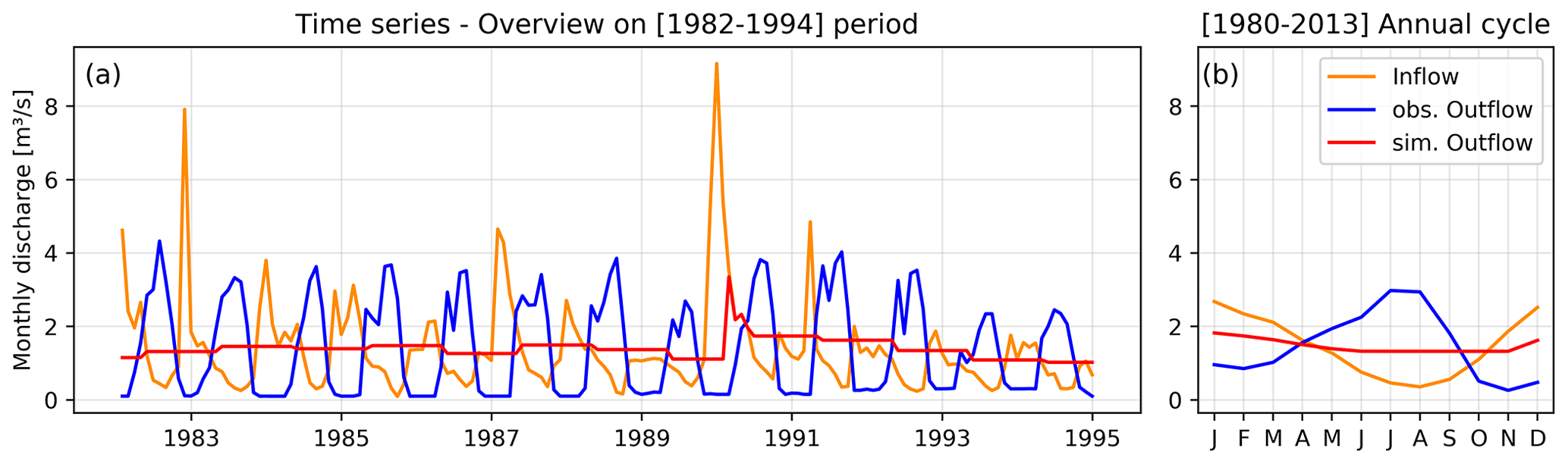
Figure 13Example of time series (a) and monthly means (b) of simulated releases from Los Bermejales reservoir, a multi-purpose reservoir primarily used for water supply and which also operates to meet irrigation water demands. The reservoir model failed to reproduce observed irrigation releases as it does not consider secondary objectives.
In addition, the model computes releases independently on each reservoir. The cascades of reservoir operations, which can be coordinated with each other, are thus not captured. More specific studies on multi-objective reservoirs (Wu and Chen, 2012; Wang et al., 2019) and multi-reservoir systems have been conducted (Chang et al., 2014; Tan et al., 2017; Rougé et al., 2021), but they all remain complex and are reservoir-specific. These methods were evaluated only at the local scale and are very difficult to extend to a global scale because they need a significant amount of observed input data and require detailed operating rule knowledge.
Regarding the representation of releases from non-irrigation reservoirs more generally, the scheme remains very simplistic since release policy is not driven by physical processes. In fact, operation rules of these types of reservoirs involve complex socioeconomic and political factors that are different in each country. Simulating other management purposes is mainly based on optimization algorithms, as is the case for hydro-power dam releases, for instance, where the objective functions are economically oriented (i.e., to maximize energy production; Moeini et al., 2011; Feng et al., 2017; Chong et al., 2021). These methods remain very reservoir-specific and are currently deemed to be too complex to be applicable at a large scale.
The model provides a relatively good performance in representing irrigation reservoir operations because of its physical approach that links water releases to crop water demands. However, some simplifications are to be noted which could be improved in the future. The irrigation water demand estimation is based on the irrigation scheme in ISBA LSM, which has its own limitations (Druel et al., 2022). Also, in this version of the reservoir scheme, water demands for each irrigation reservoir are reduced to considering pixels that are downstream of the reservoir at a given maximum distance dmax. This creates inconsistencies because water demand is not linked to the reservoir water storage capacity, which leads for some reservoirs to much higher water demands compared to water supply. Moreover, here there is no proportionality rule set between reservoirs with common irrigation grid cells. They are recorded on multiple reservoirs when their command areas are overlapping because the model runs on each reservoir independently. We end up repeatedly counting shared pixels, and this leads to overestimation of water demands at the level of each reservoir. According to results from the sensitivity analysis, parameter dmax alone (ranging from 1 to 250 km) does not have much influence on outflow variance, and this is even more true when irrigation demands are considered excessive compared to inflow (DPI ), because in that case the amount of irrigation demand is not more significant in outflow computing; only the seasonal variation defines the reservoir release curve. Zhou et al. (2021) suggested an efficient way to overcome this issue by defining a least-cost adduction network, based on Portoghese et al. (2013) and Neverre et al. (2016), to connect each irrigation grid cell to a unique abstraction point, either a river or a reservoir, by using topographic information, distance and upstream areas of the river abstraction points. This approach has the advantage of considering not only the downstream grid cells, but all the surrounding ones. Most importantly, it ensures that reservoir command areas do not overlap anymore and that each pixel irrigation demand is only counted once. The method is implemented in the routing model of ORCHIDEE (ORganizing Carbon and Hydrology In Dynamic EcosystEms; Nguyen-Quang et al., 2018) and can be easily implemented in other routing models. It is also interesting at this stage to account for all possible sources of water withdrawals, including underground water, canals, but also the abstractions made directly from the reservoirs' storage, in order to have a more realistic representation of reservoir releases.
Another aspect which is not explicitly simulated in the model is water abstraction. In this study, abstractions are taken into account indirectly since the inflow is reconstructed from observations at the inlet of each reservoir. However, once the DROP model is implemented in a hydrological model, the tributary inflows will correspond to river flows simulated by the routing model, and therefore there should be a deterioration of the performance index on discharge with an error spreading along the anthropized rivers. However, by coupling the above with a model that takes irrigation into account, such as the new version of the ISBA land surface model, for example (Druel et al., 2022), the water releases from the reservoir model can be linked to crop irrigation needs, and thus river water withdrawals can be represented as well as those taken directly from the reservoirs.
5.2 Contributions of the sensitivity analysis to a clearer understanding of the DROP model
The sensitivity analysis has revealed the most influential parameters and those that can be set using predefined values without impacting the model output uncertainty distribution. It emerged that cthreshold is the most influential parameter in representing reservoir releases, and this result is consistent with the analysis of Shin et al. (2019) on the role of the release ratio R where cthreshold is involved. Indeed, the aforementioned study showed the positive contribution of this formulation to the R ratio (R=α c, i.e., ) and its optimization in improving the representation of release and stabilizing water storage in the simulated reservoirs, especially those with (the values of c for which 4c2=α c and , α being set at 0.85).
Hanasaki et al. (2006) conducted a sensitivity test on the α parameter for a case study of a large relative capacity hydroelectric reservoir (c=2.28). The model was tested with four different values of α (0.65, 0.75, 0.85, and 0.95) and found that this parameter had a low impact on the simulated release but a high impact on the simulated storage, except when the reservoir is full. α showed high sensitivity to releases when events with water passing over spillways were more frequent. Their conclusions concerning the sensitivity to outflows are also in line with the results found here.
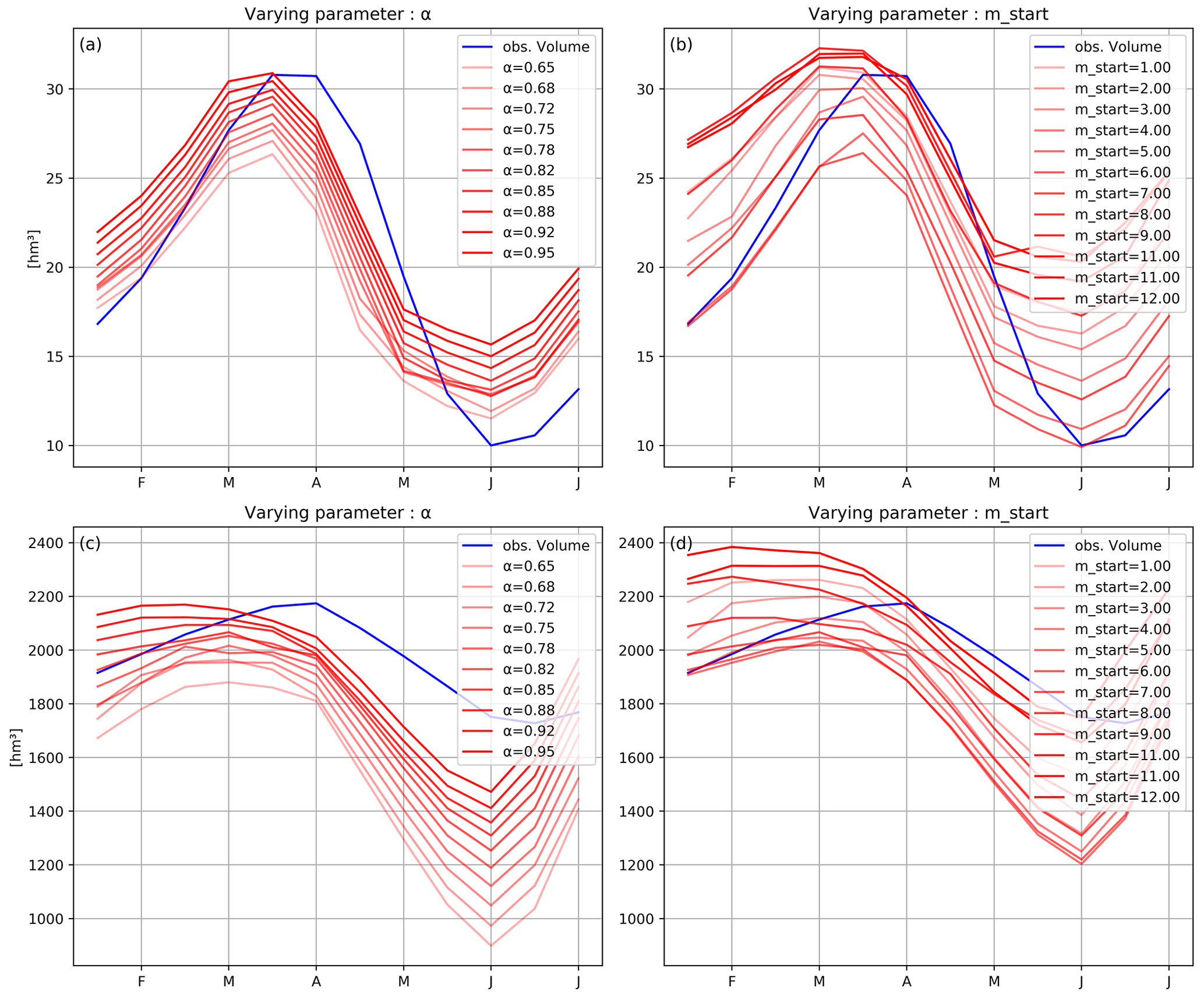
Actually, the sensitivity analysis undertaken in this study focused on the model sensitivity in the average representation of releases rather than on the filling levels of reservoirs since the focus of the study is on flow representation and the effect of anthropogenic factors in altering the flow dynamics along the rivers. If we were to focus on water resource availability and water management issues, the sensitivity analysis should also focus on the uncertainty in representing water storage levels in the reservoirs, considering the C2M over volumes as the variable of interest. In this configuration, as shown in Fig. 14, the parameters α and mstart, alongside cthreshold, will emerge as the most influential parameters with significantly high sensitivity indices of both first and total orders.
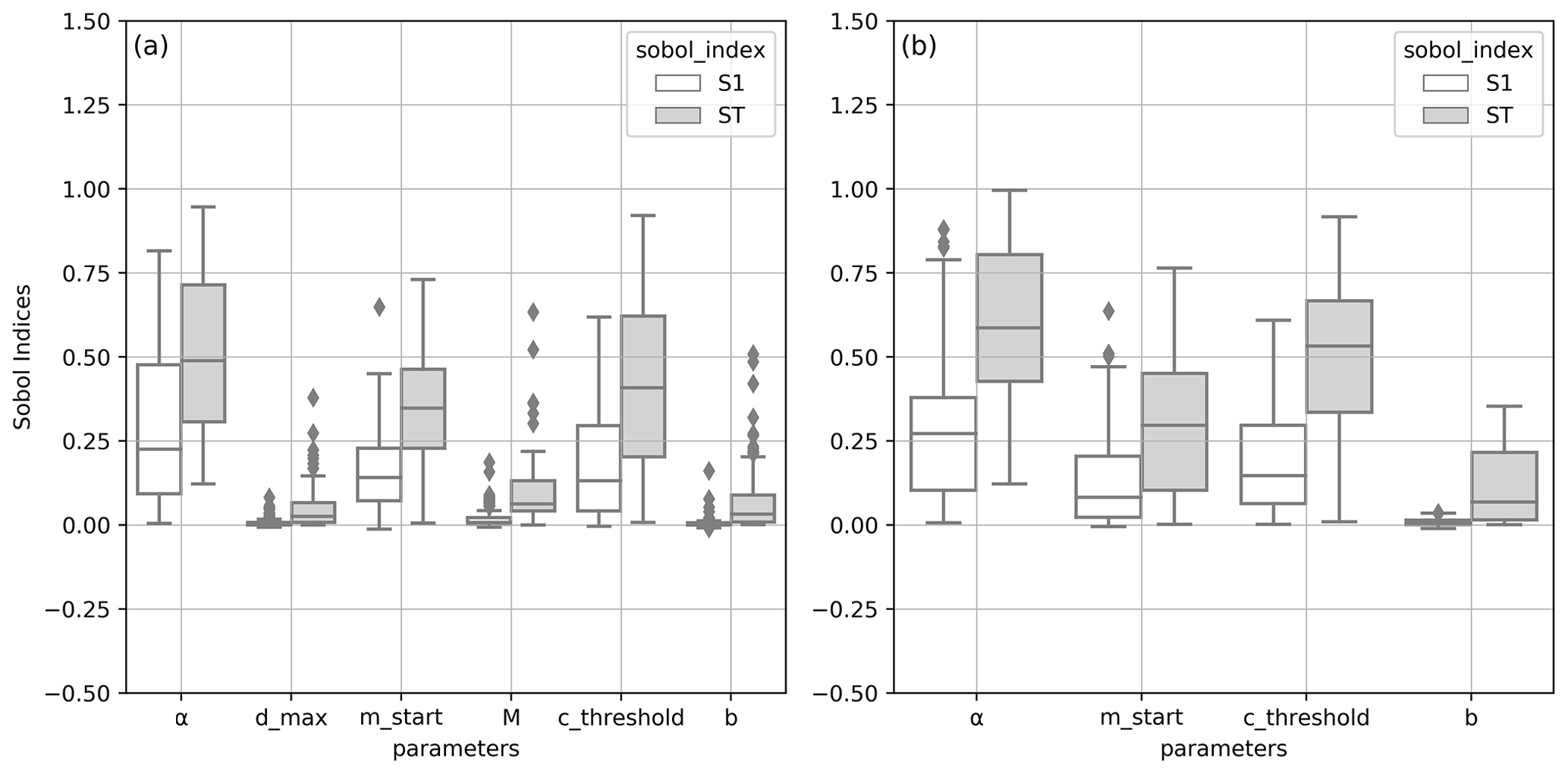
Figure 14Distribution of first- (“S1”) and total-order (“ST”) Sobol indices of parameters based on C2M variance over volumes: (a, c) in irrigation and (b, d) in non-irrigation reservoirs.
Both α and mstart directly affect the bias in the filling curve representation. In the ideal case where the reservoir state is not on the boundary conditions, the filling curve is vertically shifted following the value of α and the chosen month in order to bring the reservoir volume at the beginning of each operating year in line with the ideal filling rate α C, as shown in Fig. 15, without changing the seasonal release pattern. The larger the seasonality of reservoir water levels, the greater the effect of both parameters, which is very noticeable in large-storage capacity reservoirs used for water supply and hence explains the two parameters' interaction with cthreshold.
In this paper, a global parameterized model, DROP, was reconstructed based on the Hanasaki et al. (2006) generic scheme to represent reservoir releases in Spain. Results reveal the positive contribution of the model in representing the seasonal cycle of discharge and storage variation, specifically for irrigation large-storage capacity reservoirs, as the model succeeds in reproducing the seasonal shift between inflows and outflows, improving river flow representation (C2M improvement rate) by 123 % in the median. The results also provide a further validation of the Hanasaki et al. (2006) formulation on 215 reservoirs in Spain where reliable observed data are readily accessible. While Spain represented an idealized case study in terms of data availability, different remote sensing data will allow the extension of the model to any other river basin over the globe, more specifically to those which are ungauged, since the reservoir model relies only on the GRanD reservoir database (which is global). This work is in preparation for the upcoming SWOT wide-swath altimetry mission (Biancamaria et al., 2016), which will provide the data necessary to make improved global-scale river and reservoir storage and flow estimates. Furthermore, the results highlight the importance of incorporating reservoir operations into large-scale hydrological models for a more realistic representation of river flows and thus the water mass exchange with oceans and the atmosphere. The physical approach of DROP is consistent with that of the ISBA-CTRIP LSM RRM (land surface–river routing model): irrigation demands used as input to the reservoir model can be simulated by the irrigation module recently integrated into ISBA (Druel et al., 2022), and CTRIP already includes a lake model, “MLake” (Guinaldo et al., 2021), that a priori models inland water bodies at a global scale, calculates mass balance and lake outflow at the global scale, and provides the foundation for integrating human reservoir operations. The next step is to implement the DROP model in MLake and create a link between the two anthropization models by coupling the new versions of ISBA (irrigation) and CTRIP (reservoirs).
The sensitivity analysis, based on Sobol's method, was conducted on the C2M representation of the mean seasonal outflow patterns. The results show that the most important parameter overall is cthreshold. M and dmax are ranked second, in the median, in terms of irrigation reservoir release representation, and their importance is linked to the reservoir relative capacity. α and mstart have less influence on both types of reservoir outflow seasonal dynamics but are important if the focus is on reservoir water storage values. It has also been proven that the significance of the model's parameters varies according to the range of reservoir relative capacities being studied. The results represent an essential step to further improve either river flow modeling or reservoir water storage, through calibration schemes and assimilation of new remote sensing products, by targeting the most influential reservoir model parameters. A supplementary application of this work is provided as a calibration study of the model over Spain (see Supplement). This work provides future studies with a fully generalized parameterization of the reservoir scheme along with a deeper insight into the way each of the parameters influences the model outputs and how their importance changes depending on the reservoir characteristics and the output variable of interest.
Overall, integrating this reservoir model into LSM RRMs, which are in turn coupled to climate and Earth system models (such as the CNRM-CM and CNRM-ESM; Voldoire et al., 2019; Séférian et al., 2019), will provide a major advance in understanding past climate reanalysis and will enable a more realistic representation of future scenarios under climate change.
The DROP model and the sensitivity analysis codes are available on Zenodo. Post-processing codes are also available. All information can be found in the following repository: https://doi.org/10.5281/zenodo.6389405 (Sadki, 2022).
The supplement related to this article is available online at: https://doi.org/10.5194/gmd-16-427-2023-supplement.
MS, SM, AB and SR designed the study and determined the methodology. MS and SM developed the reservoir model and the sensitivity analysis algorithm. MS performed the analysis and wrote the original draft. All the authors contributed to the editing and review of the paper.
The contact author has declared that none of the authors has any competing interests.
Publisher's note: Copernicus Publications remains neutral with regard to jurisdictional claims in published maps and institutional affiliations.
We would like to thank Pere Quintana-Segui from Ebro Observatory for providing the SAFRAN-based meteorological dataset for Spain which was used to force the ISBA LSM and compute irrigation demands. We also thank him for providing pre-processed products of the in situ natural and anthropized flow and volume observations over Spain.
This study is part of Malak Sadki's thesis work, co-funded by the French National Center for Space Studies (CNES) and the Occitania Region in France.
This paper was edited by Min-Hui Lo and reviewed by three anonymous referees.
Abdolghafoorian, A. and Farhadi, L.: Uncertainty quantification in land surface hydrologic modeling: Toward an integrated variational data assimilation framework, IEEE J. Sel. Top. Appl. Earth Obs., 9, 2628–2637, https://doi.org/10.1109/JSTARS.2016.2553444, 2016. a
AQUASTAT: FAO's Global Information System on Water and Agriculture, https://www.fao.org/aquastat/ (last access: 16 February 2022), 1994. a
Batalla, R. J., Gomez, C. M., and Kondolf, G. M.: Reservoir-induced hydrological changes in the Ebro River basin (NE Spain), J. Hydrol., 290, 117–136, 2004. a
Baumgartner, A. and Reichel, E.: The world water balance: mean annual global, continental and maritime precipitation and run-off, Elsevier, CRID 1573668924526185088, 1975. a
Biancamaria, S., Lettenmaier, D. P., and Pavelsky, T. M.: The SWOT mission and its capabilities for land hydrology, in: Remote sensing and water resources, Springer International Publishing, 117–147, https://doi.org/10.1007/978-3-319-32449-4_6, 2016. a
Biemans, H., Haddeland, I., Kabat, P., Ludwig, F., Hutjes, R., Heinke, J., von Bloh, W., and Gerten, D.: Impact of reservoirs on river discharge and irrigation water supply during the 20th century, Water Resour. Res., 47, https://doi.org/10.1029/2009WR008929, 2011. a, b, c, d
Borgonovo, E.: A new uncertainty importance measure, Reliab. Eng. Syst. Safe., 92, 771–784, 2007. a
Borgonovo, E. and Plischke, E.: Sensitivity analysis: a review of recent advances, Eur. J. Oper. Res., 248, 869–887, 2016. a
Calvet, J.-C. and Champeaux, J.-L.: L'apport de la télédétection spatiale à la modélisation des surfaces continentales, La Météorologie, 2020, 52–58, 2020. a
Chang, J., Meng, X., Wang, Z., Wang, X., and Huang, Q.: Optimized cascade reservoir operation considering ice flood control and power generation, J. Hydrol., 519, 1042–1051, 2014. a
Chao, B. F., Wu, Y.-H., and Li, Y.: Impact of artificial reservoir water impoundment on global sea level, Science, 320, 212–214, 2008. a
Chong, K. L., Lai, S. H., Ahmed, A. N., Jaafar, W. Z. W., and El-Shafie, A.: Optimization of hydropower reservoir operation based on hedging policy using Jaya algorithm, Appl. Soft Comput., 106, 107325, https://doi.org/10.1016/j.asoc.2021.107325, 2021. a
Chun, M.-H., Han, S.-J., and Tak, N.-I.: An uncertainty importance measure using a distance metric for the change in a cumulative distribution function, Reliab. Eng. Syst. Safe., 70, 313–321, 2000. a
Coerver, H. M., Rutten, M. M., and van de Giesen, N. C.: Deduction of reservoir operating rules for application in global hydrological models, Hydrol. Earth Syst. Sci., 22, 831–851, https://doi.org/10.5194/hess-22-831-2018, 2018. a
Decharme, B., Delire, C., Minvielle, M., Colin, J., Vergnes, J.-P., Alias, A., Saint-Martin, D., Séférian, R., Sénési, S., and Voldoire, A.: Recent changes in the ISBA-CTRIP land surface system for use in the CNRM-CM6 climate model and in global off-line hydrological applications, J. Adv. Model. Earth Sy., 11, 1207–1252, 2019. a
Döll, P., Fiedler, K., and Zhang, J.: Global-scale analysis of river flow alterations due to water withdrawals and reservoirs, Hydrol. Earth Syst. Sci., 13, 2413–2432, https://doi.org/10.5194/hess-13-2413-2009, 2009. a, b, c
Downing, J. A., Prairie, Y. T., Cole, J. J., Duarte, C. M., Tranvik, L. J., Striegl, R. G., McDowell, W. H., Kortelainen, P., Caraco, N. F., Melack, J. M., and Middelburg, J. J.: The global abundance and size distribution of lakes, ponds, and impoundments, Limnol. Oceanogr., 51, 2388–2397, 2006. a
Druel, A., Munier, S., Mucia, A., Albergel, C., and Calvet, J.-C.: Implementation of a new crop phenology and irrigation scheme in the ISBA land surface model using SURFEX_v8.1, Geosci. Model Dev., 15, 8453–8471, https://doi.org/10.5194/gmd-15-8453-2022, 2022. a, b, c, d, e, f
Dynesius, M. and Nilsson, C.: Fragmentation and flow regulation of river systems in the northern third of the world, Science, 266, 753–762, 1994. a
Ehsani, N., Fekete, B. M., Vörösmarty, C. J., and Tessler, Z. D.: A neural network based general reservoir operation scheme, Stoch. Env. Res. Risk A., 30, 1151–1166, 2016. a
Feng, M., Liu, P., Guo, S., Shi, L., Deng, C., and Ming, B.: Deriving adaptive operating rules of hydropower reservoirs using time-varying parameters generated by the E n KF, Water Resour. Res., 53, 6885–6907, 2017. a
Frederikse, T., Landerer, F., Caron, L., Adhikari, S., Parkes, D., Humphrey, V. W., Dangendorf, S., Hogarth, P., Zanna, L., Cheng, L., and Wu, Y.-H.: The causes of sea-level rise since 1900, Nature, 584, 393–397, 2020. a
Grill, G., Lehner, B., Lumsdon, A. E., MacDonald, G. K., Zarfl, C., and Liermann, C. R.: An index-based framework for assessing patterns and trends in river fragmentation and flow regulation by global dams at multiple scales, Environ. Res. Lett., 10, 015001, https://doi.org/10.1088/1748-9326/10/1/015001, 2015. a
Grill, G., Lehner, B., Thieme, M., Geenen, B., Tickner, D., Antonelli, F., Babu, S., Borrelli, P., Cheng, L., Crochetiere, H., Ehalt Macedo, H., Filgueiras, R., Goichot, M., Higgins, J., Hogan, Z., Lip, B., McClain, M. E., Meng, J., Mulligan, M., Nilsson, C., Olden, J. D., Opperman, J. J., Petry, P., Reidy Liermann, C., Sáenz, L., Salinas-Rodríguez, S., Schelle, P., Schmitt, R. J. P., Snider, J., Tan, F., Tockner, K., Valdujo, P. H., van Soesbergen, A., and Zarfl, C.: Mapping the world’s free-flowing rivers, Nature, 569, 215–221, 2019. a, b
Guinaldo, T., Munier, S., Le Moigne, P., Boone, A., Decharme, B., Choulga, M., and Leroux, D. J.: Parametrization of a lake water dynamics model MLake in the ISBA-CTRIP land surface system (SURFEX v8.1), Geosci. Model Dev., 14, 1309–1344, https://doi.org/10.5194/gmd-14-1309-2021, 2021. a
Gutenson, J. L., Tavakoly, A. A., Wahl, M. D., and Follum, M. L.: Comparison of generalized non-data-driven lake and reservoir routing models for global-scale hydrologic forecasting of reservoir outflow at diurnal time steps, Hydrol. Earth Syst. Sci., 24, 2711–2729, https://doi.org/10.5194/hess-24-2711-2020, 2020. a, b
Haddeland, I., Skaugen, T., and Lettenmaier, D. P.: Anthropogenic impacts on continental surface water fluxes, Geophys. Res. Lett., 33, https://doi.org/10.1029/2006GL026047, 2006. a, b, c
Hanasaki, N., Kanae, S., and Oki, T.: A reservoir operation scheme for global river routing models, J. Hydrol., 327, 22–41, 2006. a, b, c, d, e, f, g, h, i, j, k, l, m, n, o, p, q, r, s
Hanasaki, N., Kanae, S., Oki, T., Masuda, K., Motoya, K., Shirakawa, N., Shen, Y., and Tanaka, K.: An integrated model for the assessment of global water resources – Part 1: Model description and input meteorological forcing, Hydrol. Earth Syst. Sci., 12, 1007–1025, https://doi.org/10.5194/hess-12-1007-2008, 2008. a
Herman, J.: Usher W, SALib: An open-source Python library for Sensitivity Analysis, JOSS, 2, 97, https://doi.org/10.21105/joss.00097, 2017. a
Herrera, P. A., Marazuela, M. A., and Hofmann, T.: Parameter estimation and uncertainty analysis in hydrological modeling, Wiley Interdisciplinary Reviews: Water, 9, e1569, https://doi.org/10.1002/wat2.1569, 2022. a
Hoeffding, W.: A class of statistics with asymptotically normal distribution, in: Breakthroughs in statistics, Springer, New York, NY, 308–334, 1992. a
Horan, R., Rickards, N. J., Kaelin, A., Baron, H. E., Thomas, T., Keller, V. D. J., Mishra, P. K., Nema, M. K., Muddu, S., Garg, K. K., Pathak, R., Houghton-Carr, H. A., Dixon, H., Jain, S. K., and Rees, G.: Extending a large-scale model to better represent water resources without increasing the model's complexity, Water, 13, 3067, https://doi.org/10.3390/w13213067, 2021. a
Huang, C., Tong, J., and Ye, M.: Global sensitivity analysis for a prediction model of soil solute transfer into surface runoff, J. Hydrol., 599, 126342, https://doi.org/10.1016/j.jhydrol.2021.126342, 2021. a
ICOLD: International Commission of Large Dams (ICOLD) (2020), World Register of Dams, Int. Comm. Large Dams, Paris, France, https://www.icold-cigb.org/ (last access: 25 January 2022), 2020. a, b
IEA: International Energy Agency, https://www.iea.org/data-and-statistics/data-tables?country=SPAIN&energy=Electricity&year=2020, last access: 31 January 2022. a
INE: Instituto Nacional de Estadística. España, https://www.ine.es/explica/explica_infografias.htm, last access: 31 January 2022. a
Lehner, B., Liermann, C. R., Revenga, C., Vörösmarty, C., Fekete, B., Crouzet, P., Döll, P., Endejan, M., Frenken, K., Magome, J., et al.: High-resolution mapping of the world's reservoirs and dams for sustainable river-flow management, Front. Ecol. Environ., 9, 494–502, 2011. a, b, c, d
Le Moigne, P., Colin, J., and Decharme, B.: Impact of lake surface temperatures simulated by the FLake scheme in the CNRM-CM5 climate model, Tellus A, 68, 31274, https://doi.org/10.3402/tellusa.v68.31274, 2016. a
Liu, Y. and Gupta, H. V.: Uncertainty in hydrologic modeling: Toward an integrated data assimilation framework, Water Resour. Res., 43, https://doi.org/10.1029/2006WR005756, 2007. a
López-Moreno, J. I., Vicente-Serrano, S. M., Beguería, S., García-Ruiz, J. M., Portela, M. M., and Almeida, A.: Dam effects on droughts magnitude and duration in a transboundary basin: The Lower River Tagus, Spain and Portugal, Water Resour. Res., 45, https://doi.org/10.1029/2008WR007198, 2009. a
Lorenzo-Lacruz, J., Vicente-Serrano, S. M., López-Moreno, J. I., Beguería, S., García-Ruiz, J. M., and Cuadrat, J. M.: The impact of droughts and water management on various hydrological systems in the headwaters of the Tagus River (central Spain), J. Hydrol., 386, 13–26, 2010. a
Lorenzo-Lacruz, J., Vicente-Serrano, S. M., López-Moreno, J. I., Morán-Tejeda, E., and Zabalza, J.: Recent trends in Iberian streamflows (1945–2005), J. Hydrol., 414, 463–475, 2012. a, b
Maier, H. R. and Dandy, G. C.: Neural networks for the prediction and forecasting of water resources variables: a review of modelling issues and applications, Environ. Model. Softw., 15, 101–124, 2000. a
Mathevet, T., Michel, C., Andréassian, V., and Perrin, C.: A bounded version of the Nash-Sutcliffe criterion for better model assessment on large sets of basins, in: Large sample basin experiments for hydrological model parameterisation: Results of the Model Parameter Experiment – MOPEX, edited by: Andréas-sian, V., Hall, A., Chahinian, N., and Schaake, J., IAHS Red Books Series no. 307, IAHS, Wallingford, UK, 211–219, 2006. a
Moeini, R., Afshar, A., and Afshar, M.: Fuzzy rule-based model for hydropower reservoirs operation, Int. J. Elec. Power, 33, 171–178, 2011. a
Munier, S. and Decharme, B.: River network and hydro-geomorphological parameters at ∘ resolution for global hydrological and climate studies, Earth Syst. Sci. Data, 14, 2239–2258, https://doi.org/10.5194/essd-14-2239-2022, 2022. a, b
Nash, J. E. and Sutcliffe, J. V.: River flow forecasting through conceptual models part I – A discussion of principles, J. Hydrol., 10, 282–290, 1970. a
Neverre, N., Dumas, P., and Nassopoulos, H.: Large-scale water scarcity assessment under global changes: insights from a hydroeconomic framework, Hydrol. Earth Syst. Sci. Discuss. [preprint], https://doi.org/10.5194/hess-2015-502, in review, 2016. a
Nguyen-Quang, T., Polcher, J., Ducharne, A., Arsouze, T., Zhou, X., Schneider, A., and Fita, L.: ORCHIDEE-ROUTING: revising the river routing scheme using a high-resolution hydrological database, Geosci. Model Dev., 11, 4965–4985, https://doi.org/10.5194/gmd-11-4965-2018, 2018. a
Oki, T. and Kanae, S.: Global hydrological cycles and world water resources, Science, 313, 1068–1072, 2006. a
Pheulpin, L., Bertrand, N., and Bacchi, V.: Uncertainty quantification and global sensitivity analysis with dependent inputs parameters: Application to a basic 2D-hydraulic model, LHB, 108, 2015 265, 2022. a
Pianosi, F., Beven, K., Freer, J., Hall, J. W., Rougier, J., Stephenson, D. B., and Wagener, T.: Sensitivity analysis of environmental models: A systematic review with practical workflow, Environ. Model. Softw., 79, 214–232, 2016. a
Pokhrel, Y. N., Hanasaki, N., Yeh, P. J., Yamada, T. J., Kanae, S., and Oki, T.: Model estimates of sea-level change due to anthropogenic impacts on terrestrial water storage, Nat. Geosci., 5, 389–392, 2012. a
Portoghese, I., Bruno, E., Dumas, P., Guyennon, N., Hallegatte, S., Hourcade, J.-C., Nassopoulos, H., Pisacane, G., Struglia, M. V., and Vurro, M.: Impacts of climate change on freshwater bodies: quantitative aspects, in: Regional Assessment of Climate Change in the Mediterranean, Advances in Global Change Research, vol. 50, Springer, Dordrecht, 241–306, https://doi.org/10.1007/978-94-007-5781-3_9, 2013. a
Quintana-Seguí, P., Turco, M., Herrera, S., and Miguez-Macho, G.: Validation of a new SAFRAN-based gridded precipitation product for Spain and comparisons to Spain02 and ERA-Interim, Hydrol. Earth Syst. Sci., 21, 2187–2201, https://doi.org/10.5194/hess-21-2187-2017, 2017. a
Raman, H. and Chandramouli, V.: Deriving a general operating policy for reservoirs using neural network, J. Water Resour. Plan. Manag., 122, 342–347, 1996. a
Razavi, S. and Karamouz, M.: Adaptive neural networks for flood routing in river systems, Water Int., 32, 360–375, 2007. a
Revenga, C., Campbell, I., Abell, R., De Villiers, P., and Bryer, M.: Prospects for monitoring freshwater ecosystems towards the 2010 targets, Philos. T. Roy. Soc. B, 360, 397–413, 2005. a
Rougé, C., Reed, P. M., Grogan, D. S., Zuidema, S., Prusevich, A., Glidden, S., Lamontagne, J. R., and Lammers, R. B.: Coordination and control – limits in standard representations of multi-reservoir operations in hydrological modeling, Hydrol. Earth Syst. Sci., 25, 1365–1388, https://doi.org/10.5194/hess-25-1365-2021, 2021. a
Sadki, M.: Implementation and sensitivity analysis of a Dam-Reservoir OPeration model (DROP v1.0) over Spain – Supplement, Zenodo [code], https://doi.org/10.5281/zenodo.6389405, 2022. a
Saltelli, A.: Making best use of model evaluations to compute sensitivity indices, Comput. Phys. Commun., 145, 280–297, 2002. a
Saltelli, A.: The cautious modeller: craftsmanship without wizardry. Preface to “Analyse de sensibilité et exploration de modèles. Applications aux modèles environnementaux”, edited by: Faivre, R., Iooss, B., Mahévas, S., Makowski, D., and Monod, H., Edition QUAE, 352 p., Collection Savoir-Faire, ISBN 978-2-7592-1906-3, 2013. a
Saltelli, A. and Annoni, P.: How to avoid a perfunctory sensitivity analysis, Environ. Model. Softw., 25, 1508–1517, 2010. a
Saltelli, A., Ratto, M., Andres, T., Campolongo, F., Cariboni, J., Gatelli, D., Saisana, M., and Tarantola, S.: Global sensitivity analysis: the primer, John Wiley & Sons, ISBN 9780470725177, 2008. a, b
Saltelli, A., Annoni, P., Azzini, I., Campolongo, F., Ratto, M., and Tarantola, S.: Variance based sensitivity analysis of model output. Design and estimator for the total sensitivity index, Comput. Phys. Commun., 181, 259–270, 2010. a
Séférian, R., Nabat, P., Michou, M., Saint-Martin, D., Voldoire, A., Colin, J., Decharme, B., Delire, C., Berthet, S., Chevallier, M., Sénési, S., Franchisteguy, L., Vial, J., Mallet, M., Joetzjer, E., Geoffroy, O., Guérémy, J.-F., Moine, M.-P., Msadek, R., Ribes, A., Rocher, M., Roehrig, R., Salas-y-Mélia, D., Sanchez, E., Terray, L., Valcke, S., Waldman, R., Aumont, O., Bopp, L., Deshayes, J., Éthé, C., and Madec, G.: Evaluation of CNRM earth system model, CNRM-ESM2-1: Role of earth system processes in present-day and future climate, J. Adv. Model. Earth Sy., 11, 4182–4227, 2019. a
Shin, M.-J. and Jung, Y.: Using a global sensitivity analysis to estimate the appropriate length of calibration period in the presence of high hydrological model uncertainty, J. Hydrol., 607, 127546, https://doi.org/10.1016/j.jhydrol.2022.127546, 2022. a
Shin, S., Pokhrel, Y., and Miguez-Macho, G.: High-resolution modeling of reservoir release and storage dynamics at the continental scale, Water Resour. Res., 55, 787–810, 2019. a, b, c, d, e, f, g, h, i, j, k, l, m
Sobol, I. M.: Sensitivity analysis for non-linear mathematical models, Mathematical modelling and computational experiment, Mathematical modelling and computational experiment, 1, 407–414, 1993. a
Syed, T. H., Famiglietti, J. S., Chambers, D. P., Willis, J. K., and Hilburn, K.: Satellite-based global-ocean mass balance estimates of interannual variability and emerging trends in continental freshwater discharge, P. Natl. Acad. Sci. USA, 107, 17916–17921, 2010. a
Tan, Q.-f., Wang, X., Wang, H., Wang, C., Lei, X.-h., Xiong, Y.-S., and Zhang, W.: Derivation of optimal joint operating rules for multi-purpose multi-reservoir water-supply system, J. Hydrol., 551, 253–264, 2017. a
Tang, Y., Reed, P., Van Werkhoven, K., and Wagener, T.: Advancing the identification and evaluation of distributed rainfall-runoff models using global sensitivity analysis, Water Resour. Res., 43, https://doi.org/10.1029/2006WR005813, 2007a. a
Tang, Y., Reed, P., Wagener, T., and van Werkhoven, K.: Comparing sensitivity analysis methods to advance lumped watershed model identification and evaluation, Hydrol. Earth Syst. Sci., 11, 793–817, https://doi.org/10.5194/hess-11-793-2007, 2007b. a
Van Beek, L., Wada, Y., and Bierkens, M. F.: Global monthly water stress: 1. Water balance and water availability, Water Resour. Res., 47, https://doi.org/10.1029/2010WR009791, 2011. a
Vanderkelen, I., Gharari, S., Mizukami, N., Clark, M. P., Lawrence, D. M., Swenson, S., Pokhrel, Y., Hanasaki, N., van Griensven, A., and Thiery, W.: Evaluating a reservoir parametrization in the vector-based global routing model mizuRoute (v2.0.1) for Earth system model coupling, Geosci. Model Dev., 15, 4163–4192, https://doi.org/10.5194/gmd-15-4163-2022, 2022. a
Voldoire, A., Saint-Martin, D., Sénési, S., Decharme, B., Alias, A., Chevallier, M., Colin, J., Guérémy, J.-F., Michou, M., Moine, M.-P., Nabat, P., Roehrig, R., Salas y Mélia, D., Séférian, R., Valcke, S., Beau, I., Belamari, S., Berthet, S., Cassou, C., Cattiaux, J., Deshayes, J., Douville, H., Ethé, C., Franchistéguy, L., Geoffroy, O., Lévy, C., Madec, G., Meurdesoif, Y., Msadek, R., Ribes, A., Sanchez-Gomez, E., Terray, L., and Waldman, R.: Evaluation of CMIP6 deck experiments with CNRM-CM6-1, J. Adv. Model. Earth Sy., 11, 2177–2213, 2019. a
Vörösmarty, C. J., Meybeck, M., Fekete, B., Sharma, K., Green, P., and Syvitski, J. P.: Anthropogenic sediment retention: major global impact from registered river impoundments, Global Planet. Change, 39, 169–190, 2003. a
Wada, Y., de Graaf, I. E., and van Beek, L. P.: High-resolution modeling of human and climate impacts on global water resources, J. Adv. Model. Earth Sy., 8, 735–763, 2016. a
Wang, K., Shi, H., Chen, J., and Li, T.: An improved operation-based reservoir scheme integrated with Variable Infiltration Capacity model for multiyear and multipurpose reservoirs, J. Hydrol., 571, 365–375, 2019. a
Wu, Y. and Chen, J.: An operation-based scheme for a multiyear and multipurpose reservoir to enhance macroscale hydrologic models, J. Hydrometeorol., 13, 270–283, 2012. a
Yassin, F., Razavi, S., Elshamy, M., Davison, B., Sapriza-Azuri, G., and Wheater, H.: Representation and improved parameterization of reservoir operation in hydrological and land-surface models, Hydrol. Earth Syst. Sci., 23, 3735–3764, https://doi.org/10.5194/hess-23-3735-2019, 2019. a
Young Jr., G. K.: Finding reservoir operating rules, J. Hydraul. Div., 93, 297–322, 1967. a
Zamanian, S., Hur, J., and Shafieezadeh, A.: Significant variables for leakage and collapse of buried concrete sewer pipes: A global sensitivity analysis via Bayesian additive regression trees and Sobol’indices, Struct. Infrastruct. E., 17, 676–688, 2021. a
Zhang, C., Chu, J., and Fu, G.: Sobol′’s sensitivity analysis for a distributed hydrological model of Yichun River Basin, China, J. Hydrol., 480, 58–68, 2013. a, b
Zhao, T., Yang, D., Cai, X., Zhao, J., and Wang, H.: Identifying effective forecast horizon for real-time reservoir operation under a limited inflow forecast, Water Resour. Res., 48, https://doi.org/10.1029/2011WR010623, 2012. a
Zhou, X., Polcher, J., and Dumas, P.: Representing human water management in a land surface model using a supply/demand approach, Water Resour. Res., 57, e2020WR028133, https://doi.org/10.1029/2020WR028133, 2021. a
Zouhri, W., Homri, L., and Dantan, J.-Y.: Handling the impact of feature uncertainties on SVM: a robust approach based on Sobol sensitivity analysis, Expert Syst. Appl., 189, 115691, https://doi.org/10.1016/j.eswa.2021.115691, 2022. a