the Creative Commons Attribution 4.0 License.
the Creative Commons Attribution 4.0 License.
 | 27 Jul 2023
Description and evaluation of the JULES-ES set-up for ISIMIP2b
Camilla Mathison
Eleanor Burke
Andrew J. Hartley
Douglas I. Kelley
Chantelle Burton
Eddy Robertson
Nicola Gedney
Karina Williams
Andy Wiltshire
Richard J. Ellis
Alistair A. Sellar
Chris D. Jones
Global studies of climate change impacts that use future climate model projections also require projections of land surface changes. Simulated land surface performance in Earth system models is often affected by the atmospheric models' climate biases, leading to errors in land surface projections. Here we run the Joint UK Land Environment Simulator Earth System configuration (JULES-ES) land surface model with the Inter-Sectoral Impact Model Intercomparison Project second-phase future projections (ISIMIP2b) bias-corrected climate model data from four global climate models (GCMs). The bias correction reduces the impact of the climate biases present in individual models. We evaluate the performance of JULES-ES against present-day observations to demonstrate its usefulness for providing required information for impacts such as fire and river flow. We include a standard JULES-ES configuration without fire as a contribution to ISIMIP2b and JULES-ES with fire as a potential future development. Simulations for gross primary productivity (GPP), evapotranspiration (ET) and albedo compare well against observations. Including fire improves the simulations, especially for ET and albedo and vegetation distribution, with some degradation in shrub cover and river flow. This configuration represents some of the most current Earth system science for land surface modelling. The suite associated with this configuration provides a basis for past and future phases of ISIMIP, providing a simulation set-up, postprocessing and initial evaluation, using the International Land Model Benchmarking (ILAMB) project. This suite ensures that it is as straightforward, reproducible and transparent as possible to follow the protocols and participate fully in ISIMIP using JULES.
- Article
(7779 KB) - Full-text XML
-
Supplement
(2172 KB) - BibTeX
- EndNote


The works published in this journal are distributed under the Creative Commons Attribution 4.0 License. This license does not affect the Crown copyright work, which is re-usable under the Open Government Licence (OGL). The Creative Commons Attribution 4.0 License and the OGL are interoperable and do not conflict with, reduce or limit each other.
© Crown copyright 2022
The Joint UK Land Environment Simulator (JULES; Clark et al., 2011; Best et al., 2011) is a community-supported and developed land surface model used by land, hydrological, weather and climate communities. JULES is a configurable code base supporting weather, climate and Earth system science applications. Here, we describe and evaluate the JULES Earth System (JULES-ES) configuration and experimental set-up used in the Inter-Sectoral Impact Model Intercomparison Project (ISIMIP; Frieler et al., 2017). JULES-ES builds on the JULES-GL7 configuration described in Wiltshire et al. (2020) by including additional biogeochemical fluxes governing carbon and nitrogen cycles that influence Earth system processes; these are considered to be more relevant to ecosystems and people, which could be affected by climate change. While we run JULES-ES in offline mode, it is also coupled to the atmosphere within the Earth system model UKESM (Sellar et al., 2019). Climate change impacts are already a feature of everyday life for much of the world, and quantifying these allows us to understand future benefits and trade-offs of climate mitigation and adaptation policies. ISIMIP provides a consistent framework for assessing impacts, using a large ensemble of impacts models across various sectors (Warszawski et al., 2013, 2014). ISIMIP has recently completed its second phase, having more than 60 modelling groups contributing simulations to ISIMIP2a (reanalysis-driven hindcasts) and ISIMIP2b (bias-corrected global-climate-model-driven historical and future scenarios). We present the JULES-ES configuration and experimental set-up that has contributed to ISIMIP2b and will be the basis for further development in subsequent ISIMIP phases. An advantage of using JULES-ES as an offline impact model is that it uses a prescribed atmosphere; without these feedbacks, JULES-ES is 10 000–20 000 times more computationally efficient than the closely aligned land surface scheme coupled to the atmosphere in UKESM1 (Sellar et al., 2019), and, in using a multi-model climate ensemble, it samples scientific uncertainty in our understanding of the climate system that would not be possible within a single climate model framework.
This paper briefly describes the changes to JULES-GL7 (Wiltshire et al., 2020) that form the JULES-ES configuration, the ISIMIP set-up and an evaluation of the arising simulations. JULES-ES has been widely evaluated and applied for global biogeochemical modelling (Sellar et al., 2019; Slevin et al., 2017), including in the Global Carbon Budget (Friedlingstein et al., 2020). Here we focus on using JULES for impact applications. Alongside this work, we provide a suite to run JULES-ES, following the ISIMIP2b modelling protocol (Frieler et al., 2017) for tailored impact projections that are consistent across sectors such as water and biomes. The suite includes the code to postprocess output into ISIMIP formatted netCDF output and run the International Land Model Benchmarking (ILAMB) system to allow quick evaluation (see Sect. S1). Data from the JULES-ES ISIMIP2b suite have been submitted to the biomes and water ISIMIP2b sectors, are available via the ISIMIP model archive (https://data.isimip.org/, last access: 27 June 2023) and provide simulations of the historical and future land surface in the Popescu et al. (2022) wildfire report. The JULES ISIMIP2b simulations with fire provide the basis for the contribution of JULES to the next Fire Model Intercomparison Project (FireMIP), which will use the ISIMIP3 set-up. The historical simulations and their evaluation are shown in Sect. 3, with the discussion and conclusions in Sects. 4 and 5, respectively.
2.1 JULES-ES configuration
To better represent the variation in plant traits and managed land, we extend the standard representation of 5 plant functional types (PFTs) to 13 in JULES-ES, building on Harper et al. (2016), with 4 managed and 9 natural PFTs. Natural PFTs are extended by splitting trees into deciduous and evergreen types and then distinguishing between temperate and tropical broadleaf evergreen trees. These additional PFTs represent a wider range of leaf lifespans and metabolic capacities. Evergreen trees typically have less access to nutrients, higher leaf mass per unit area, longer lifespans and lower carbon assimilation and respiration rates, whereas a deciduous PFT typically has leaves with a higher nutrient concentration, shorter lifespan and lower leaf mass per unit area. Tropical broadleaf evergreen trees have lower maximum carbon assimilation rates than temperate trees. The nine natural PFTs used are tropical broadleaf evergreen trees (BET-Tr), temperate broadleaf evergreen trees (BET-Te), broadleaf deciduous trees (BDT), needleleaf evergreen trees (NET), needleleaf deciduous trees (NDT), C3 grasses (C3G), C4 grasses (C4G), evergreen shrubs (ESh) and deciduous shrubs (DSh). Harper et al. (2016) also updated several parameters required for calculating photosynthesis and respiration using the TRY database (Kattge et al., 2011). They also reduced the bias in model simulations by tuning parameters relating to leaf dark respiration, canopy radiation, canopy nitrogen, stomatal conductance, root depth, and temperature sensitivities of the maximum carboxylation rate of RuBisCO (Vcmax) based on available observations. The four managed PFTs are C3 and C4 crop and pasture (C3Cr, C4Cr, C3Pa and C4Pa) PFTs and are functionally similar to natural grasses, but, in the case of crops, are assumed not to be nitrogen limited, and litter carbon is removed as a simple representation of crop harvest (Sellar et al., 2019; Robertson, 2019). This simple fertilisation of crops through lack of nitrogen limitation does not make a distinction between mineral and manure fertiliser. Both crop and pasture surface types undergo land use change according to externally forced time-varying land use, but the pasture is not grazed and is otherwise unmanaged. Within the respective crop and pasture fraction, only the C3 and C4 crop and pasture PFTs are allowed to grow, with the area of each determined by the TRIFFID dynamic vegetation module (Burton et al., 2019).
Outside of the managed land area, the nine natural PFTs (including natural C3 grasses and C4 grasses) can grow in the remainder of the grid box once the non-vegetated surfaces have been accounted for (urban, ice and lakes, represented by corresponding non-vegetation surface types, and ocean, which is not simulated). As the net prescribed crop or pasture fraction increases with land use change, natural vegetation is removed from the portion of the grid box into which agriculture has expanded, representing anthropogenic land clearance. Conversely, when crop and pasture areas are reduced, the natural PFTs are allowed to recolonise the vacated grid box fraction. The vacated grid box fraction is initially bare soil, and the existing natural PFTs gradually expand their coverage into this area; the rate of expansion is determined by the TRIFFID vegetation dynamics scheme and will follow a succession of faster-growing grass PFTs, followed by shrubs and then trees. Bare soil occupies any remaining space, once the vegetation dynamics have been simulated. Simple representations of fertilisation and harvesting are applied to the crop PFTs, but otherwise, these are physiologically identical to the natural grasses. After accounting for land use, the fractional coverage and biomass of each PFT within a grid box is determined by the TRIFFID dynamic vegetation model. Inter-PFT competition is based on vegetation height, with the taller vegetation shading and therefore dominating other PFTs (Harper et al., 2018).
The other major change introduced in JULES-ES is a representation of nitrogen and nutrient limitation effects on ecosystem carbon assimilation. The nitrogen component of JULES is described in Wiltshire et al. (2021). In brief, JULES-ES represents all the key terrestrial nitrogen processes. Inputs to the land surface are via biological fixation, fertilisation and nitrogen deposition, with losses from the land surface occurring via leaching and gas loss, with nitrogen deposition being externally provided to the model. JULES simulates a nitrogen-limited ecosystem by reducing the carbon use efficiency if there is insufficient available nitrogen to satisfy plant nitrogen demand. This results in a reduced net primary production (NPP) when we include nitrogen limitation. The soil biogeochemistry is based on the representation of the four-pool RothC soil carbon (Clark et al., 2011), consisting of decomposable plant material (DPM), resistant plant material (RPM), microbial biomass (BIO), and humus (HUM). For each soil carbon pool, there is an equivalent soil nitrogen pool (Wiltshire et al., 2021). Nitrogen transfers between the organic and inorganic nitrogen pools depend on decomposition rates and the carbon to nitrogen ratio of the organic pool.
Another important change is the inclusion of a fire module. Fire is simulated in JULES by the fire model INFERNO (INteractive Fire and Emission algoRithm for Natural envirOnments; Mangeon et al., 2016). Burnt area is calculated from flammability and ignitions. Temperature, saturation vapour pressure, relative humidity and precipitation, together with the soil moisture and fuel load from JULES, give flammability by PFT and the prescribed population density (Klein Goldewijk et al., 2017) gives human ignitions, while the prescribed climatological lightning gives natural ignitions. Previous evaluation of JULES-INFERNO, which compared model output against observational constraints, showed that the burnt area is relatively insensitive to changes in lightning (Mangeon et al., 2016; Burton et al., 2022). Here we use INFERNO coupled to the dynamic vegetation model TRIFFID (Burton et al., 2019), enabling carbon cycle feedbacks from fire onto the land surface via vegetation mortality, regrowth and burnt litter fluxes. Recent updates to INFERNO allow fire mortality to vary by PFT, and updates to the representation of land use and PFTs in JULES allow for reduced burning in C3 crop and C4 crop PFTs (Burton et al., 2020), based on global trends of agricultural fire suppression (Bistinas et al., 2014; Andela et al., 2017). Background mortality rates were reduced compared to the model without fire to account for the extra vegetation mortality from fire, as per Burton et al. (2019). We use fire and background mortality in Burton et al. (2020). C3 pasture and C4 pasture burn at the same rate as natural grasses, as per Burton et al. (2019), which reflects observational constraints that show an increase in burnt area for pasture areas (Kelley et al., 2019; Bistinas et al., 2014).
2.2 Modifications for ISIMIP2b
In JULES with dynamical vegetation switched on, the TRIFFID period is a number (in days) that defines the frequency at which the TRIFFID dynamic vegetation code is called. In the ISIMIP JULES-ES configuration, it has been reduced from a 10 to a 1 d period to allow for shorter restart periods, which were necessary to meet the diagnostic requirements of ISIMIP (a large number of variables on short temporal scales). A daily TRIFFID period also allows the vegetation dynamics to respond more realistically to variations in plant productivity on shorter timescales, although the effect of this change is minimal in test historical runs.
Another key difference to the standard set-up of JULES is the use of daily meteorological driving data. JULES needs a model time step of no more than 1 h to accurately simulate the diurnal cycle and exchange of heat, water and momentum and to avoid numerical instabilities. In the ISIMIP experimental set-up, we use the internal disaggregation (Williams and Clark, 2014) to calculate driving data values at the model time step of 1 h. The method uses the IMOGEN model disaggregation (Huntingford et al., 2010) to initially disaggregate to every 3 h, which the model linearly interpolates to 1 h. The diurnal cycle of downward shortwave radiation is calculated from the position of the Sun in the sky. Temperature is calculated from a sinusoidal function, with a maximum 0.15 of a day's length after local noon and normalised by the diurnal temperature range. Downward longwave radiation is a linear function of temperature, and specific humidity is kept below saturation at each time step. Precipitation is considered to occur in a single event, with a globally specified duration parameter (6 h for convective rainfall, 1 h for large-scale rainfall and convective snowfall and large-scale snowfall). Convective rainfall occurs when temperature exceeds 288.15 K. The model assumes convective rainfall is more intense and so leads to more runoff and less infiltration into the soil. Given that precipitation events do not, by construction, overlap with midnight (GMT) on average, this produces a spurious trapezoidal diurnal cycle, which is zero at midnight (GMT; Williams and Clark, 2014). Precipitation above 350 mm d−1 is redistributed. Note that convective precipitation occurs only on a fraction of the grid box (Best et al., 2011), set to 30 % in the ISIMIP2b runs and, within this fraction, is modelled as a negative exponential distribution (Dolman and Gregory, 1992). Therefore, the grid box average intensity is not the same as the effective intensity at a point. Given the strong effect of intensity on canopy interception and runoff, the water cycle in the model is sensitive to the duration parameter choices (Williams and Clark, 2014).
2.3 ISIMIP2b protocol
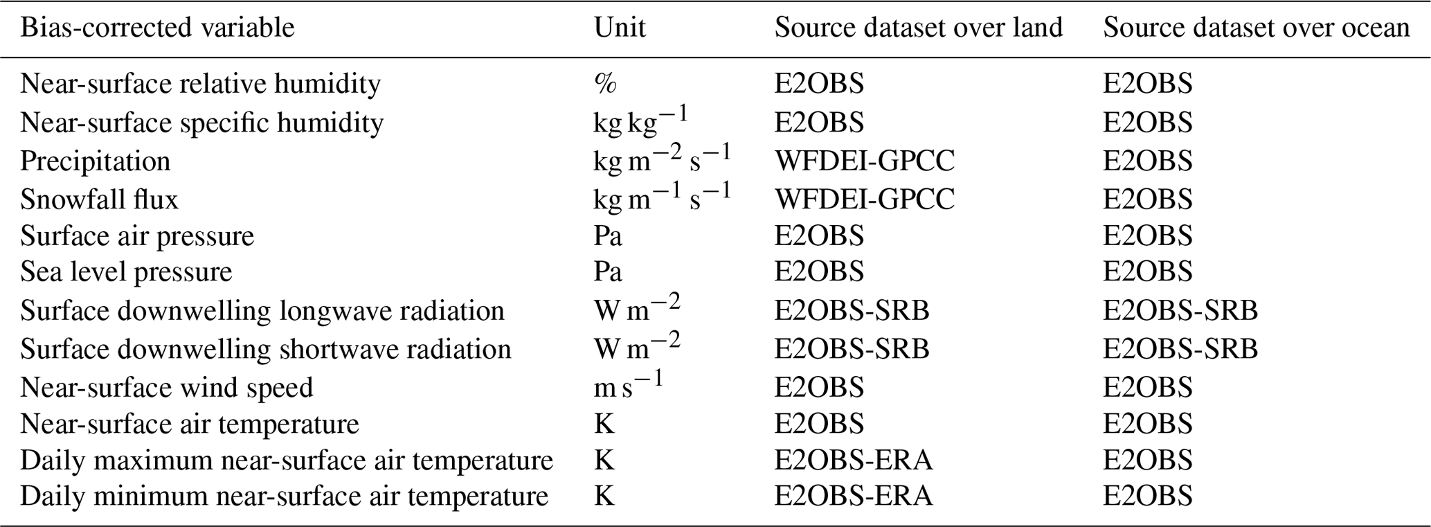
The ISIMIP2b experiments focus on understanding different levels of mitigation. They use two Representative Concentration Pathway (RCP) scenarios to explore the international commitments made under the Paris Agreement to stabilise global warming at well below 2 ∘C, relative to preindustrial mean temperatures. ISIMIP2b uses simulations from the Coupled Model Intercomparison Project 5 (CMIP5), using an historical scenario (1860–2005) and the RCP2.6 and RCP6.0 concentration pathways (post-2005) to represent a higher ambition, lower temperature outcome and a low ambition pathway, respectively (Riahi et al., 2017). Land use data and population density are based on the Shared Socioeconomic Pathway (SSP2) scenario and applied to RCP2.6 and RCP6.0 simulations. Lightning ignitions for fire are from the LIS/OTD version 2.3.2015 climatology (Cecil, 2006) and applied for the historical reference period and the future, as per Rabin et al. (2017) and Hantson et al. (2020). To capture a range of climate sensitivities, the following four CMIP5 global climate model (GCM) driving models are chosen: GFDL-ESM2M, HadGEM2-ES, IPSL-CM5A-LR and MIOC5. The GCM driving data are global, bias-corrected, daily data at 0.5∘ resolution (Hempel et al., 2013; Frieler et al., 2017; Lange, 2018). Bias correction means we can compare the observed and simulated impacts during the historical reference period, with a smooth transition into the future period. The bias-correction methodology adjusts multi-year monthly mean distribution throughout the historical and RCP periods, based on comparison of GCM output against EWEMBI reanalysis data distributions (Dee et al., 2011), for the period 1979 to 2013, using CMIP5 RCP8.5 post-2005 (the end of the CMIP5 historic period), such that trends and interannual variability are preserved in absolute and relative terms for temperature and non-negative variables, respectively (Lange, 2018). EWEMBI combines data from multiple reanalysis sources to cover all the required variables. The variables bias-corrected for ISIMIP2b are listed in Table 1, as reproduced from Frieler et al. (2017). The ISIMIP2b bias correction includes humidity in addition to shortwave and longwave radiation, using quantile mapping. Transfer functions are used to adjust the distributions of daily anomalies from monthly mean values. ISIMIP2b bias-correction methods adjust distributions independently for each variable, grid cell and month, preserving the statistical dependencies between variables in space and changes over time. The bias-correction approach preserves the trends (and therefore sensitivities) from different GCMs but removes absolute biases found over the reference period from the historical and RCP periods. Each GCM therefore has a different variability and simulated climate outside of the reference period but with a smooth transition going from the historical period into the reference period or from the reference period into the future. Some small biases remain after bias correction, particularly in precipitation (Fig. S1), where biases are a small fraction of the total local rainfall but can affect precipitation particularly in the South America (Fig. S2). As part of the set-up provided here, we include code for preparing JULES data for submitting to ISIMIP and ensuring that it conforms to the strict protocols (see Sect. S1) and the ILAMB system for rapid evaluation of the simulations (see Sect. S2).
Table 1Bias-corrected variables for ISIMIP2b simulations, reproduced from Table 1 of Frieler et al. (2017).
2.4 Model evaluation
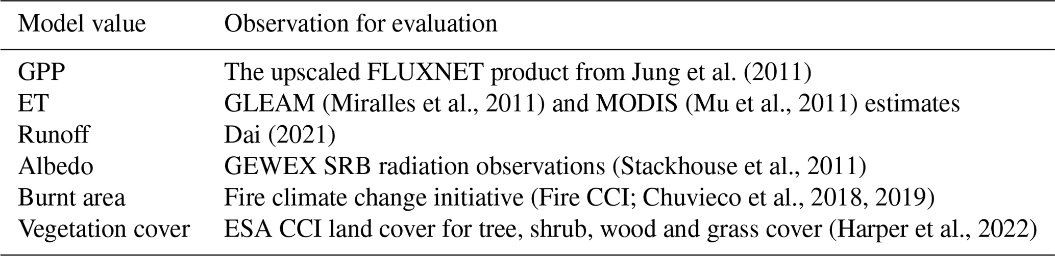
We evaluate the model for key impacts sectors and use the International Land Model Benchmarking (ILAMB) tool (Collier et al., 2018) to assess model performance for gross primary productivity (GPP), evapotranspiration (ET), runoff and albedo. ILAMB evaluates performance against observations from remote sensing, reanalysis data and FLUXNET site measurements and produces graphical and statistical scores of model results. The model values and the observation datasets we use for the evaluation are given in Table 1. As ILAMB does not include vegetation cover evaluation, we also include the Manhattan metric (Kelley et al., 2013) comparison with ESA CCI (European Space Agency Climate Change Initiative) land cover for tree, shrub, wood and grass cover (Harper et al., 2022). Results and further details of the ILAMB and vegetation cover analysis are provided in Sect. S2. We evaluate the historical simulations separately for each GCM because the bias correction preserves interannual differences between GCMs. We conduct an evaluation over common time periods between observations and simulation, using the historical period and, for observational periods beyond the end of 2006, RCP6.0.
2.5 The experimental suite
To run JULES, we collect all the tasks and input files that are needed into what is known as a suite; this allow runs to be reproduced using exactly the same applications, options and commands as previously run, possibly by another user, scheduling them to run based on the dependencies between the tasks. Full instructions on how to run JULES in a suite are provided on GitHub (https://jules-lsm.github.io/tutorial/bg_info/tutorial_julesrose/jr_structures.html#jrsuite, last access: 27 June 2023). We provide a full set-up for running the ISIMIP2b simulations using JULES-ES in the form of the suite u-cc669, which is available via the Met Office Science Repository Service (MOSRS; https://code.metoffice.gov.uk/trac/roses-u, last access: 27 June 2023; see the data availability section for more information). The bias-corrected driving data are available from ISIMIP at https://www.isimip.org/gettingstarted/input-data-bias-adjustment/ (last access: 27 June 2023). We also use the following datasets from ISIMIP. In situations in which the preprocessing of these datasets requires the use of these data within JULES, this preprocessing code is also part of the suite.
-
CO2 concentration
-
Future land use patterns
-
Nitrogen deposition
-
Land–sea mask
The Total Runoff Integrating Pathways (TRIP) river-routing model allows JULES to collect and route water through river channels, essentially converting runoff to river discharge or river flow. A TRIP 0.5∘ river-routing ancillary file is also required for these runs, which is available from http://hydro.iis.u-tokyo.ac.jp/~taikan/TRIPDATA/ (last access: 27 June 2023).
3.1 Water
We evaluated the water cycle using runoff derived from Dai (2021) for the 50 largest river catchments. Estimated observed mean basin runoff combines river flow measurements at downstream gauge stations with a river flow model to estimate the flow at the river mouth. By assuming that there are no losses from the river, we calculated the long-term mean of the basin-averaged runoff by dividing the river flow at the river mouth by the basin area.
Particularly in temperate regions north and south of the Equator, simulations using all four sets of driving data show similar biases. However, differences between the driving datasets are the greatest in tropical or sub-tropical river catchments (Fig. 1). This is particularly evident in the Amazon basin, where mean runoff biases range from approximately 0 in the simulation driven by HADGEM2-ES to more than −0.6 mm d−1 in the simulation driven by IPSL-CM5A-LR. Strong variations between the simulations are also seen in the Brahmaputra basin, with some smaller variations in the Changjiang basin (Fig. 2). The general underestimate of runoff in the higher latitudes may be due to the treatment of moisture infiltration into partially frozen soils (see below) but could also be caused by biases in precipitation estimates due to the gauge undercatch of snow (Adam and Lettenmaier, 2003). In arid and semi-arid basins, river flow and runoff tend to be overestimated, which could be due to missing processes such as river channel evaporation and transmission losses (Haddeland et al., 2011; Döll and Siebert, 2002) and anthropogenic water extraction, which is primarily irrigation (Richey et al., 2015).
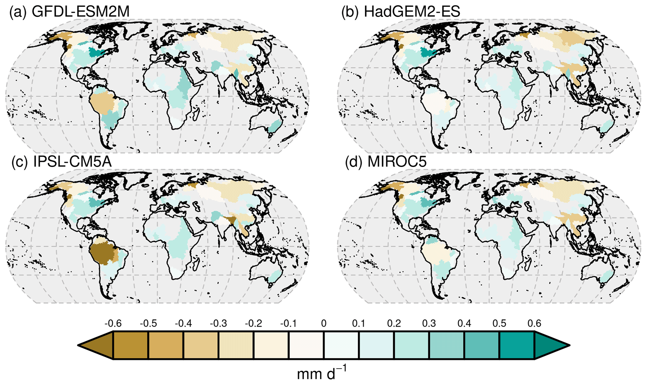
Figure 1Multi-year mean bias of catchment-scale runoff simulated by JULES driven by four sets of climate-driving data compared to runoff derived from Dai (2021). The number of years of observations contributing to the multi-year mean varies, depending on catchment and the observations that are available. Observations used are within the period 1980–2006. ISIMIP2b forcing data are derived from four CMIP5 GCMs (GFDL-ESM2M, HadGEM2-ES, IPSL-CM5A-LR and MIROC5).
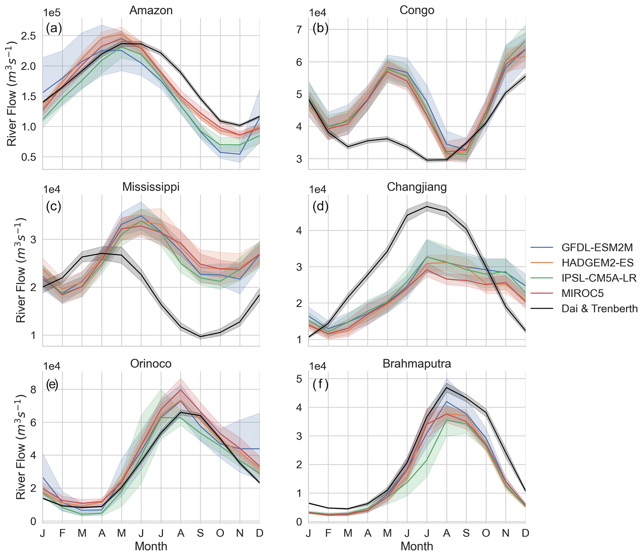
Figure 2Comparison of the simulated long-term monthly mean river flow with observations (Dai, 2021) for the six largest rivers. (a) Amazon (Óbidos; −1.95∘ N, −55.51∘ E). (b) Congo (Kinshasa; −4.3∘ N, 15.3∘ E). (e) Orinoco (Puente de Angostura ; 8.15∘ N, −63.6∘ E). (d) Changjiang (Datong; 30.77∘ N, 117.62∘ E). (f) Brahmaputra (Bahadurabad; 25.18∘ N, 89.67∘ E). (c) Mississippi (Vicksburg; 32.31∘ N, −90.91∘ E). The observations are over the time period from 1980 to 2010.
Figure 2 compares the long-term monthly mean river flow (1980–2014 inclusive, where observations are available) over the six largest rivers to those of the downstream observations in Dai (2021). All the simulations reproduce the overall seasonal river flow over the Amazon. After the wet season, the modelled river flows decline earlier than observed, and the simulated river flows at low water are too low. This could be due to too much evaporation in the drier months (see JJA in Fig. S3) and/or the simulated speed of flow through the soil and/or river channel being too fast, although GFDL-ESM2M and IPSL-CM5A-LR driving precipitation data also have a dry bias during the dry season (Fig. S2). All simulations overestimate river flow over the Democratic Republic of the Congo (hereafter abbreviated as Congo), mainly due to overestimates in the rainy months. This could be driven by too little evaporation from the vegetation canopy or from flooded areas (see ET in Figs. 3 and S3). The simulations reproduce the seasonal river flow over the Orinoco well. The timings of peak river flow for the Changjiang and Brahmaputra are well simulated, although the amplitudes are too low. Dams, which we do not model, are likely to affect the observed seasonal cycle. The simulated river flow over the Mississippi lags observations by several months. This lag is also evident over many high-latitude basins (not shown). The observed river flow peak is mainly driven by spring melt, whereas the simulated river flow peak is in line with that of precipitation. This is due to this configuration allowing significant soil infiltration of snowmelt when the soil surface is mainly frozen, rather than resulting in surface runoff. This may also result in the underestimate of annual river flow because once the water has infiltrated the soil then it may then be evaporated.
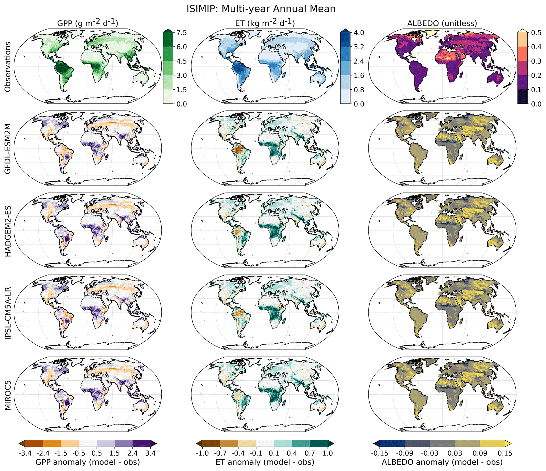
Figure 3Multi-year annual mean for GPP (column 1), evapotranspiration (column 2) and albedo (column 3) for observations (row 1), and subsequent rows show the anomaly compared with observations for each set of ISIMIP2b forcing data derived from GFDL-ESM2M (row 2), HADGEM2-ES (row 3), IPSL-CM5A-LR (row 4) and MIROC5 (row 5). Observations have been downloaded from ILAMB (https://www.ilamb.org/doc/ilamb_fetch.html, last access: 27 June 2023), and the datasets shown are GBAF for GPP (Jung et al., 2011), GLEAM for ET (Miralles et al., 2011) and GEWEX SRB for albedo (Stackhouse et al., 2011).
3.2 Surface fluxes
Global gross primary productivity (GPP) is 134–137 PgC yr−1, depending on driving data, which is above the estimate of IPCC AR6 (Canadell et al., 2021) of 113 PgC yr−1 but agrees well with the estimates of 146 ± 21 PgC yr−1 in Cheng et al. (2017; Table S1). Net biome productivity (NBP) is 0.94–1.46 PgC yr−1 between 2011–2020, within the 1.0–2.8 PgC yr−1 range estimated by the Global Carbon Budget (Friedlingstein et al., 2022). All simulations show positive GPP biases in similar regions, such as central and southern Africa, south of the Himalaya and east towards Bangladesh and Myanmar, compared to the observations in Jung et al. (2011; Fig. 3). South America is a more complicated picture, with Brazil broadly split between negative GPP to the northeast and positive GPP to the country's southeast. For Brazil, the ET bias has a more northwest–southeast split, with the northwest having a slightly negative bias and the southeast more positive. The northwest bias in ET and the bias in GPP in South America is more prominent and widespread in early wet season (September–November) when driven by climate data from GFDL-ESM2M and IPSL-CM5A-LR (see Fig. S4) and is due to a longer dry season in both sets of driving data (Fig. S2), with rains starting in October rather than September. The areas in the far north of Columbia, Bolivia and Argentina also have a negative bias in both GPP and ET across the simulations. Australia also has a north–south split, with a slightly positive ET bias to the north and the inverse to the south.
Albedo (Fig. 3; right column) generally shows a positive bias across most regions and simulations. However, there are small regions with a negative bias, for example, south of the Sahel and small regions at higher northern latitudes. Eastern Siberia has a positive bias in all simulations (see Sect. 4).
3.3 Biomes
All simulations show similar vegetation cover patterns that largely follow observations, capturing high tree cover fractions in boreal and tropical forests, grass cover in tropical, temperate and boreal grasslands and bare ground in arid regions (Fig. 4). There are, however, some biases common to all simulations. The tree cover fraction is too high globally, with a simulated range of 4.97–5.31 Mkm2, which is higher than the observations and depends on driving data (Table S2). Shrub cover and grasses dominate eastern Siberian taiga in the model instead of the observed high tree cover (Fig. 4). There is also slightly too much shrub cover in tropical forests at the expense of tree cover, contributing to a global bias in shrub cover of 1.22–1.31 Mkm2. Conversely, simulated tropical tree cover is too high in savanna regions, giving the impression of more continuous and fewer fragmented forests across the tropics (Fig. 4). Boundaries between temperate and warm temperate forests and tropical forests are too sharp, suggesting that JULES-ES does not capture processes in temperate woodland transition. Savanna and grasslands tend to be too narrow, with more bare soil in the models in semi-arid regions such as southern Africa, the Mojave Desert and the Sahel.
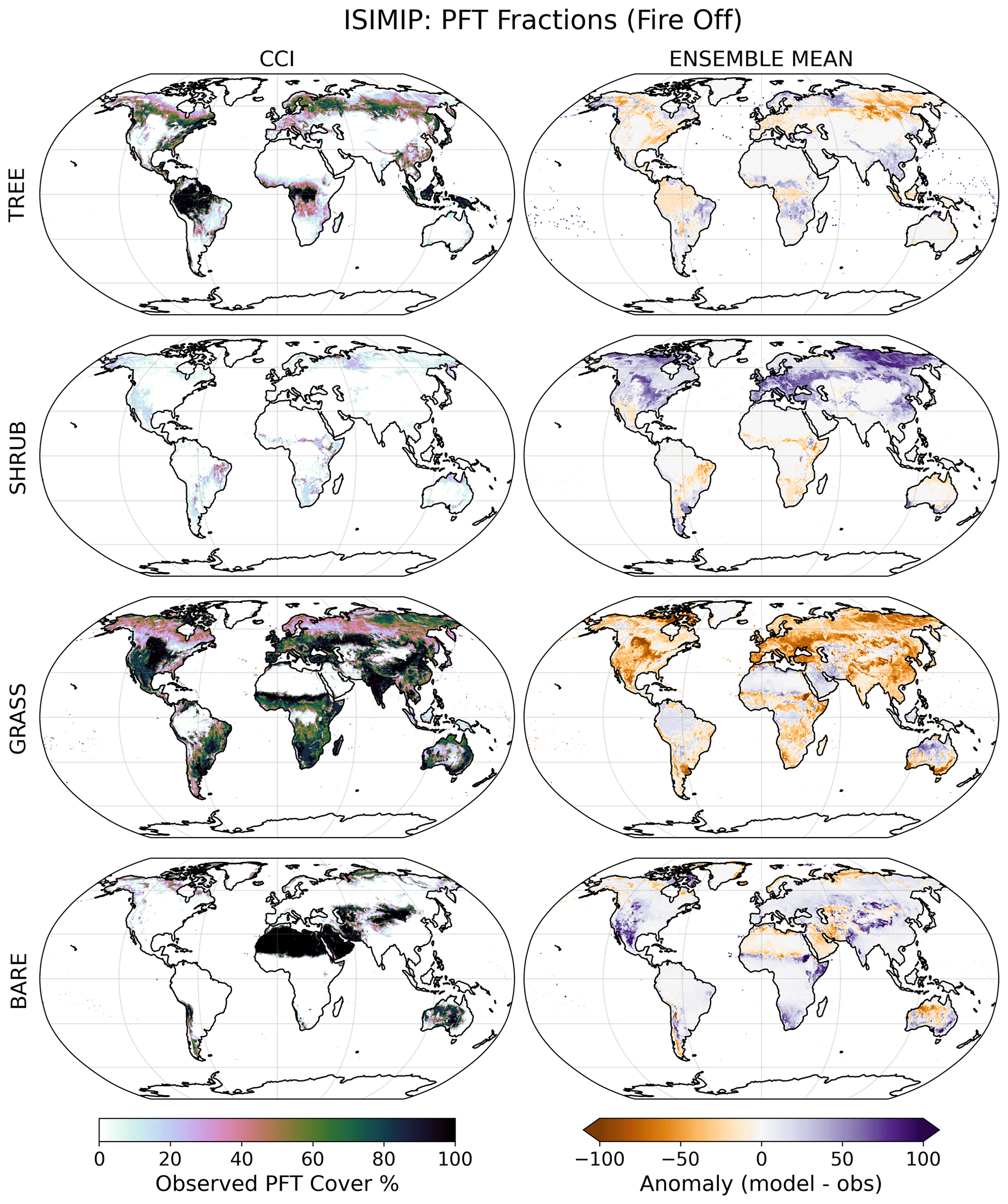
Figure 4Observed vegetation fractional cover. The first column is derived from ESA CCI land cover (v2.0.7) for 2010 (Harper et al., 2022). The second column is the difference between the observations and the simulated ensemble mean. Top to bottom rows show the tree, shrub, grass and unvegetated (bare) fraction.
3.4 Fire
In addition to the simulations without fire submitted to the archive, we performed additional simulations with fire and fire feedbacks switched on. These fire simulations provide burnt area and alter vegetation cover, carbon, fluxes, albedo and runoff (Burton et al., 2019). Burnt area is similar across all four simulations (Fig. 5). The model simulates the present-day burnt area well compared to satellite observations, with the global total burnt area average for 2000–2020 observed by MODIS CCI v5.1 as being 4.55 Mkm2, and the model simulating between 3.94 and 4.43 Mkm2, depending on the driving data (Table S3). The model captures the high burnt area in southern hemispheric Africa – a common area of low bias in global fire models (Hantson et al., 2020). The model also performs better than other FireMIP models at simulating the high burnt areas in northern hemispheric Africa, though fire is still lower than in the observations. This is partly due to very low simulated burnt areas in Nigeria's Guinean savanna, which Kelley et al. (2019) show is a consequence of global parameterisations of population density and agricultural drivers of burnt area.
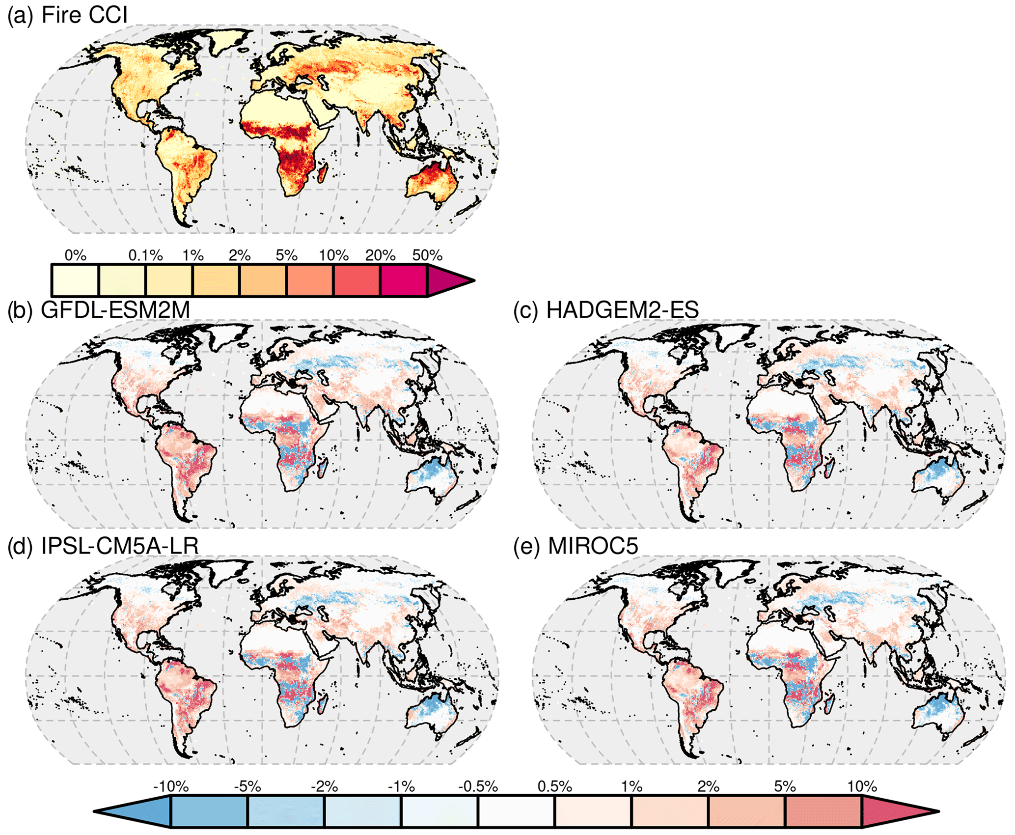
Figure 5Present-day percentage of burnt area (2000–2020) from fire CCI observations (a) (Chuvieco et al., 2018, 2019) and modelled by JULES, driven by GFDL-ESM2M (b), HadGEM2-ES (c), IPSL-CM5A-LR (d) and MIROC5 (e).
We also show an area in Australia that is burnt too little, which is a common problem across fire models (Hantson et al., 2020), even in models optimised to burnt area observations (Kelley et al., 2019; Bistinas et al., 2014). This may be due to the unique fire ecology in northern Australia (Kelley, 2014) and to high uncertainty in observations of burnt area (Giglio et al., 2010). High burning in South America occurs in areas where cropland fragmentation reduces the burnt area beyond the extent of agricultural areas (Kelley et al., 2019; Andela et al., 2017), which is hard to reproduce in tile- and PFT-based models (Hantson et al., 2016). We also simulate an area that is burnt too little in Eurasia. Some of the observed burnt areas at these high latitudes come from peatland fires, which, as in most other fire models (Rabin et al., 2017), are not simulated in INFERNO. Observational burnt area products tend to underestimate the levels of burning in forests (Randerson et al., 2012), which may explain the slight bias towards burnt areas that are simulated to be too high in tropical forests.
Fire is simulated well in savanna bands (15∘ N and 15∘ S), which improves the representation of tree cover by reducing the positive bias compared to observations (Fig. 6; Table S2). The inclusion of interactive fire has the overall effect of decreasing simulated global tree cover (from 38.66–39, depending on driving data to 34.32–35.65 Mkm2) to be more in line with the observations (34.86 Mkm2) and increasing grasses and bare soil. In the tropics, this tends to bring the modelled forest (areas dominated by trees) to being more in line with the observations, with high simulated tree cover restricted to observed forested areas. However, including fire does reduce tree cover in savanna areas (Fig. S5), particularly in Africa, which means the spatial distribution of trees in this region compared with observations is not as good as without fire (Table S2). There is an increase and improvement in tree cover in some high-latitude North American areas due to changes in background mortality in the with-fire simulation. Fire reduces shrub cover to well below observations (Table S2), though given the well-documented issues in distinguishing tall and short woody vegetation (Gerard et al., 2017; Adzhar et al., 2022), it is probably more meaningful to assess total woody cover. Here, including fire reduces model bias (from 6.19 to 6.59 to −3.60 to −2.25 Mkm2) and improves the spatial pattern (Table S2). Including fire reduces the global bias of high GPP when compared against estimations by the Global Carbon Budget (Friedlingstein et al., 2020), bringing global total down by ∼ 2 PgC yr−1 across all simulations (Table S1). However, fire does slightly degrade the GPP spatial pattern (Table S1). Including fire also reduced global NBP (Table S1) by 0.12–0.38 PgC yr−1, depending on driving data.
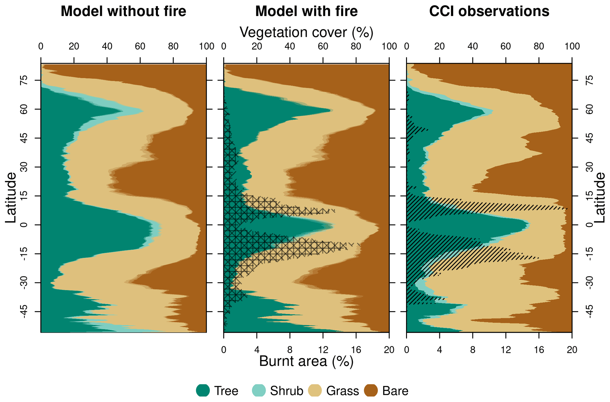
Figure 6Modelled vegetation cover without fire (left) and with fire (middle) compared to observations from ESA CCI land cover and fire (right). Dark green, light green, light brown and dark brown indicate the tree, shrub, grass and unvegetated fraction of the latitude band. The shaded transition between colours indicates the ensemble range, which is quite narrow, indicating agreement across ensemble members. Black hashing indicates the burnt area, with observations taken from MODIS CCI v5.1 (Chuvieco et al., 2018). In the middle column, the burnt area from the four driving models is shown by hatching at four different angles.
Fire alleviates some of the high bias in ET, improving the model's overall performance (Table S4). Without fire, in semi-arid areas we already overestimate river flow (probably due, in part, to human extraction). The addition of fire lowers ET, thereby increasing river flow bias in semi-arid regions, which slightly degrades overall runoff performance (Fig. S6). Fire also improves spatial pattern of albedo (Table S5), though seasonal performance decreases. This is in line with well-documented biases in fire seasonal cycles across all global fire models, which tend to have longer-than-observed fire seasons in tropical savanna, and in human-dominated fire regimes, the season timing shifts and is often late compared to observations (Hantson et al., 2016, 2020). Previous evaluations of JULES configurations incorporating INFERNO also show these biases (Burton et al., 2019, 2022, 2023; Hantson et al., 2020).
We have presented simulations of the JULES-ES land surface model, run according to the ISIMIP2b protocols using bias-corrected climate model data from four GCMs for the historical period. The configuration will be used to perform simulations under two future scenarios (RCP2.6 and RCP6.0). The JULES-ES ISIMIP2b configuration simulates the surface fluxes (GPP, ET and albedo) reasonably well. Including fire improves the ET and albedo but not the GPP, which is biased to be high. Including fire in the simulations currently degrades the runoff (Table S6).
The configurations of JULES can capture the seasonal cycle of many of the largest rivers, although high-latitude rivers and managed rivers are generally not captured as well. Including irrigation and structural hydrological developments, such as dams and reservoirs, would likely improve the simulations of managed rivers. Previously, Falloon et al. (2011) found that GCM precipitation biases contribute to errors in TRIP river flows for some basins in both HadGEM1 and HadCM3. In this study, we use bias-corrected data, which reduces these errors, meaning that differences in JULES-ES results between the driving models are due to differences in inter-seasonal or interannual variability between driving models (e.g. Fig. S2). However, errors in evapotranspiration, runoff generation or other missing processes e.g. snow accumulation and snowmelt processes, could also contribute. Uncertainty in precipitation due to the sparsity of observation networks and the undercatch of solid precipitation for high-latitude (Falloon et al., 2011) and high-altitude rivers, for example, in the Himalaya (Mathison et al., 2015), means that it is difficult to interpret model performance in these basins.
Some basins show the same bias direction in runoff (Fig. 1) and ET (Fig. 3); it is notable that the Amazon is too dry for both variables and the Nile too wet, whereas we would expect opposing biases if they were from land surface simulation. In these basins, there is a dry and wet bias (respectively) in the driving precipitation data (Fig. S1). HadGEM2-ES and IPSL-CM5A-LR have particularly dry driving data in the Amazon, and this results in the driest runoff and ET in the simulation. This translates to biases in GPP (Fig. 3) and vegetation cover (Fig. 4). So, while ISIMIP bias correction reduces climate model biases compared to those in an Earth system model (see evaluation in Sellar et al., 2019) or when run with a non-bias-corrected climate (Burton et al., 2022), they are not eliminated.
Land cover is an important factor for the surface fluxes. Grassy regions, for example, correlate with the regions of positive ET bias. The annual mean global GPP biases are small, but this is not the case for GPP on a seasonal timescale and over a smaller region such as South America. The albedo and land cover area bias are also closely related. For example, if JULES simulates a larger number of trees than observed, then this may lead to a lower albedo than observed, and vice versa. Conversely, higher grass cover just north of the Sahel corresponds to simulated low-albedo biases. Vegetation impacts on albedo are particularly important at high latitudes, where there is snow cover; for example, the positive albedo bias in eastern Siberia is because JULES simulates too few trees and too much grass there. Grasses are more readily buried below snow than trees, making these areas more reflective (Sellar et al., 2019), which in turn affects the albedo. JULES represents the bending and partial burying of vegetation by snow (Ménard et al., 2014); however, the settings controlling this interaction described in Sellar et al. (2019) have been tuned for the coupled UKESM1 model rather than the standalone JULES model. Eastern Siberia is a vulnerable region, which has experienced increased climate-related impacts, including heatwaves (Ciavarella et al., 2021) and fires (Kelley et al., 2019); it is very likely that climate change will exacerbate these feedbacks by the end of the 21st century (Popescu et al., 2022). Developments by Mercado et al. (2018), which improve the representation of plant acclimation to thermal stress, may improve spatial variations across different vegetation types in JULES.
In general, the simulations with fire improve the spatial distribution of plant functional types and vegetation productivity, particularly for tropical forests, the boundary between forests and savannas, and in North America. Developing JULES to include fire processes will improve simulations for these areas and properly capture the climate impacts on vegetation cover and carbon fluxes. The results show that there are too few trees compared to observations for the western parts of Brazil. The simulations with fire improve tree cover in savanna, which is consistent with the findings of Staver et al. (2011) and Lasslop et al. (2016); however, there is still ongoing discussion around how much impact fire really has on tree cover in the savanna compared to other dry disturbances such as wind throw, heat stress and rainfall distribution (Veenendaal et al., 2018; Brovkin et al., 2009).
We have presented a configuration of JULES-ES set-up to run and generate output following the ISIMIP protocols. We provide a suite for running the simulations that includes driving data, ancillaries, postprocessing and a first-look evaluation (ILAMB) for any phase of ISIMIP. Outputs using this set-up were submitted to the biomes and water ISIMIP2b sectors, and our evaluation helps inform of any difference between JULES-ES and other models participating in ISIMIP2b. The suite also provides a starting point for further JULES-ES developments. We evaluate a set-up with the representation of fire, using the INFERNO fire model in anticipation of ISIMIP3, which will include a fire sector. We show that including fire has an impact on model results, and that it is important to include in simulations of climate impacts. While fire mostly improves model performance, it does degrade certain vegetation distributions (for example, by simulating too little larch forest) and runoff. However, fire has a substantial impact on both ecosystem composition and hydrological processes and should therefore still be included when studying impacts under changing climate and environmental conditions. Therefore, while documentation of the configuration without fire will be useful for anyone using previously submitted results, we recommend using the configuration with fire in any future JULES-ES development. Future work using this configuration and the new phases of ISIMIP will focus on using the full benefit and extent of the ISIMIP ensemble to enable more in-depth exploration of climate impacts, together with the quantification of Earth system uncertainties, co-benefits of mitigation and adaptation to climate change.
The JULES-ES for ISIMIP configuration (based on JULES version 5.5) is preserved at https://code.metoffice.gov.uk/trac/roses-u/browser/b/k/8/8/6 (last access: 27 June 2023; fire off) and https://code.metoffice.gov.uk/trac/roses-u/browser/c/f/1/3/7 (last access: 27 June 2023; fire on). JULES and associated configurations are freely available for non-commercial research use, as set out in the JULES user terms and conditions (http://jules-lsm.github.io/access_req/JULES_Licence.pdf, last access: 27 June 2023). For a comprehensive guide on how to access, install and run the configurations used in this research, we direct the reader to Appendix A in Wiltshire et al. (2020), which is available at https://gmd.copernicus.org/articles/13/483/2020/#section6. Note that in order to view and use the JULES-ES source code, access will be required from the Met Office Science Repository Service (https://code.metoffice.gov.uk/trac/home, last access: 27 June 2023) and is available to those who have signed the JULES user agreement. The easiest way to access the repository is by completing the online form to register at http://jules-lsm.github.io/access_req/JULES_access.html (last access: 27 June 2023).
The data and code used for the evaluation of the JULES-ES outputs with ILAMB in the study are available at https://www.ilamb.org/datasets.html (Collier et al., 2018) and https://github.com/rubisco-sfa/ILAMB (last access: 27 June 2023), with a New BSD 3-clause license (https://github.com/rubisco-sfa/ILAMB/blob/master/LICENSE.rst, last access: 27 June 2023)
The JULES model data output used in the model evaluation in the study are available at https://www.isimip.org/impactmodels/details/289/ (DOIs: https://doi.org/10.48364/ISIMIP.223634, Reyer et al., 2023; https://doi.org/10.48364/ISIMIP.626689, Gosling et al., 2023), using the search tag “jules-es-55” https://data.isimip.org/search/query/jules-es-55/ (last access: 27 June 2023), with a Creative Commons Attribution 4.0 International license (https://creativecommons.org/licenses/by/4.0/, last access: 27 June 2023).
© British Crown Copyright 2022, the Met Office. All rights reserved. The software is provided by the Met Office to the topical editor at Geoscientific Model Development under the software licence for peer review (use, duplication or disclosure of this code is subject to the restrictions as set forth in the aforementioned software licence for peer review). The software is provided to facilitate the peer review of this paper, “Description and Evaluation of the JULES-ES set-up for ISIMIP2b”, and should be used and distributed to authorised persons for this purpose only. The software is extracted from the Unified Model (UM) and JULES trunks, with the revisions of the MOSRS repositories corresponding to the stated version, having passed both science and code reviews according to the UM and JULES working practices.
The supplement related to this article is available online at: https://doi.org/10.5194/gmd-16-4249-2023-supplement.
CM: conceptualisation; data curation; formal analysis; investigation; methodology; project administration; software; writing – original draft; writing – review and editing. EB: conceptualisation; data curation; investigation; methodology; software; writing – original draft; writing – review and editing. AH: data curation; formal analysis; investigation; methodology; project administration; validation; visualisation; writing – original draft; writing – review and editing. DIK: formal analysis; investigation; methodology; validation; visualisation; writing – original draft; writing – review and editing. CB: data curation; methodology; formal analysis; investigation; validation; visualisation; writing – original draft; writing – review and editing. ER: formal analysis; software; validation; writing – review and editing. NG: validation; visualisation; writing – original draft; writing – review and editing. KW: methodology; writing – review and editing. AW: writing – review and editing. RJE: software; writing – review and editing. AAS: software. CDJ: validation; writing – review and editing.
The contact author has declared that none of the authors has any competing interests.
Publisher’s note: Copernicus Publications remains neutral with regard to jurisdictional claims in published maps and institutional affiliations.
This work and its contributors have been supported by the Newton Fund through the Met Office Climate Science for Service Partnership Brazil (CSSP Brazil; Chantelle Burton, Camilla Mathison, Andrew J. Hartley, Andy Wiltshire, Chris D. Jones and Nicola Gedney), the Met Office Climate Science for Service Partnership South Africa (CSSP South Africa; Andrew J. Hartley and Camilla Mathison). Camilla Mathison, Karina Williams, Andy Wiltshire, Andrew J. Hartley, Alistair A. Sellar, Eleanor Burke, Eddy Robertson and Chris D. Jones have been supported by the Met Office Hadley Centre Climate Programme funded by BEIS and Defra. The contribution by Douglas I. Kelley and Richard J. Ellis has been supported by the UK Natural Environment Research Council through the UK Earth System Modelling Project (UKESM; grant no. NE/N017951/1). Douglas I. Kelley has been additionally supported by the UK Natural Environment Research Council as part of the NC-International programme (grant no. NE/X006247/1). Eleanor Burke and Chris D. Jones have been supported by the European Union's Horizon 2020 Research and Innovation programme (grant no. 101003536; ESM2025 – Earth System Models for the Future).
This research has been supported by the Newton Fund (Met Office Climate Science for Service Partnership Brazil and Met Office Weather and Climate Science for Service Partnership South Africa), the Department for Business, Energy and Industrial Strategy, UK government (Met Office Hadley Centre Climate Programme), the Natural Environment Research Council (the UK Earth System Modelling Project – UKESM (grant no. NE/N017951/1) and NC-International programme (grant no. NE/X006247/1)) and the Horizon 2020 (ESM2025 – Earth System Models for the Future; grant no. 101003536).
This paper was edited by Sam Rabin and reviewed by two anonymous referees.
Adam, J. C. and Lettenmaier, D. P.: Adjustment of global gridded precipitation for systematic bias, J. Geophys. Res.-Atmos., 108, 4257, https://doi.org/10.1029/2002JD002499, 2003.
Adzhar, R., Kelley, D. I., Dong, N., George, C., Torello Raventos, M., Veenendaal, E., Feldpausch, T. R., Phillips, O. L., Lewis, S. L., Sonké, B., Taedoumg, H., Schwantes Marimon, B., Domingues, T., Arroyo, L., Djagbletey, G., Saiz, G., and Gerard, F.: MODIS Vegetation Continuous Fields tree cover needs calibrating in tropical savannas, Biogeosciences, 19, 1377–1394, https://doi.org/10.5194/bg-19-1377-2022, 2022.
Andela, N., Morton, D. C., Giglio, L., Chen, Y., van der Werf, G. R., Kasibhatla, P. S., DeFries, R. S., Collatz, G. J., Hantson, S., Kloster, S., Bachelet, D., Forrest, M., Lasslop, G., Li, F., Mangeon, S., Melton, J. R., Yue C., and Randerson, J. T.: A human-driven decline in global burned area, Science, 356, 1356–1362, 2017.
Best, M. J., Pryor, M., Clark, D. B., Rooney, G. G., Essery, R. L. H., Ménard, C. B., Edwards, J. M., Hendry, M. A., Porson, A., Gedney, N., Mercado, L. M., Sitch, S., Blyth, E., Boucher, O., Cox, P. M., Grimmond, C. S. B., and Harding, R. J.: The Joint UK Land Environment Simulator (JULES), model description – Part 1: Energy and water fluxes, Geosci. Model Dev., 4, 677–699, https://doi.org/10.5194/gmd-4-677-2011, 2011.
Bistinas, I., Harrison, S. P., Prentice, I. C., and Pereira, J. M. C.: Causal relationships versus emergent patterns in the global controls of fire frequency, Biogeosciences, 11, 5087–5101, https://doi.org/10.5194/bg-11-5087-2014, 2014.
Brovkin, V., Raddatz, T., Reick, C. H., Claussen, M., and Gayler, V.: Global biogeophysical interactions between forest and climate, Geophys. Res. Lett., 36, L07405, https://doi.org/10.1029/2009GL037543, 2009.
Burton, C., Betts, R., Cardoso, M., Feldpausch, T. R., Harper, A., Jones, C. D., Kelley, D. I., Robertson, E., and Wiltshire, A.: Representation of fire, land-use change and vegetation dynamics in the Joint UK Land Environment Simulator vn4.9 (JULES), Geosci. Model Dev., 12, 179–193, https://doi.org/10.5194/gmd-12-179-2019, 2019.
Burton, C., Betts, R. A., Jones, C. D., Feldpausch, T. R., Cardoso, M., and Anderson, L. O.: El Niño Driven Changes in Global Fire 2015/16, Front. Earth Sci., 8, 199, https://doi.org/10.3389/FEART.2020.00199, 2020.
Burton, C., Kelley, D. I., Jones, C. D., Betts, R. A., Cardoso, M., and Anderson, L.: South American fires and their impacts on ecosystems increase with continued emissions, Climate Resilience and Sustainability, 1, e8, https://doi.org/10.1002/cli2.8, 2022.
Burton, C., Kelley, D. I., Burke, E., Mathison, C., Jones, C. D., Betts, R., Robertson, E., Teixeira, J. C. M., Cardoso, M., and Anderson, L. O.: Fire weakens land carbon sinks before 1.5∘, in review, 2023.
Canadell, J. G., Monteiro, P. M. S., Costa, M. H., Cotrim da Cunha, L., Cox, P. M., Eliseev, A. V., Henson, S., Ishii, M., Jaccard, S., Koven, C., Lohila, A., Patra, P. K., Piao, S., Rogelj, J., Syampungani, S., Zaehle, S., and Zickfeld, K.: : Global Carbon and other Biogeochemical Cycles and Feedbacks, in: Climate Change 2021: The Physical Science Basis. Contribution of Working Group I to the Sixth Assessment Report of the Intergovernmental Panel on Climate Change, edited by: Masson-Delmotte, V., Zhai, P., Pirani, A., Connors, S. L., Péan, C., Berger, S., Caud, N., Chen, Y., Goldfarb, L., Gomis, M. I., Huang, M., Leitzell, K., Lonnoy, E., Matthews, J. B. R., Maycock, T. K., Waterfield, T., Yelekçi, O., Yu, R., and Zhou, B., Cambridge University Press, Cambridge, United Kingdom and New York, NY, USA, 673–816, https://doi.org/10.1017/9781009157896.007, 2021.
Cecil, D. J.: LIS/OTD 0.5 Degree High Resolution Monthly Climatology (HRMC), NASA Global Hydrometeorology Resource Center DAAC, Huntsville, Alabama, USA [data set], https://doi.org/10.5067/LIS/LIS-OTD/DATA303, 2006.
Cheng, L., Zhang, L., Wang, Y. P., Canadell, J. G., Chiew, F. H. S., Beringer, J., Li, L., Miralles, D. G., Piao, S., and Zhang, Y.: Recent increases in terrestrial carbon uptake at little cost to the water cycle, Nat. Commun., 8, 110, https://doi.org/10.1038/s41467-017-00114-5, 2017.
Chuvieco, E., Lizundia-Loiola, J., Pettinari, M. L., Ramo, R., Padilla, M., Tansey, K., Mouillot, F., Laurent, P., Storm, T., Heil, A., and Plummer, S.: Generation and analysis of a new global burned area product based on MODIS 250 m reflectance bands and thermal anomalies, Earth Syst. Sci. Data, 10, 2015–2031, https://doi.org/10.5194/essd-10-2015-2018, 2018.
Chuvieco, E., Pettinari, M. L., Lizundia Loiola, J., Storm, T., and Padilla Parellada, M.: ESA Fire Climate Change Initiative (Fire_cci): MODIS Fire_cci Burned Area Grid product, version 5.1, Centre for Environmental Data Analysis, CEDA Archive [data set], https://doi.org/10.5285/3628cb2fdba443588155e15dee8e5352, 2019.
Ciavarella, A., Cotterill, D., Stott, P., Kew, S., Philip, S., van Oldenborgh, G. J., Skålevåg, A., Lorenz, P., Robin, Y., Otto, F., Hauser, M., Seneviratne, S. I., Lehner, F., and Zolina, O.: Prolonged Siberian heat of 2020 almost impossible without human influence, Climatic Change, 166, 9, https://doi.org/10.1007/S10584-021-03052-W, 2021.
Clark, D. B., Mercado, L. M., Sitch, S., Jones, C. D., Gedney, N., Best, M. J., Pryor, M., Rooney, G. G., Essery, R. L. H., Blyth, E., Boucher, O., Harding, R. J., Huntingford, C., and Cox, P. M.: The Joint UK Land Environment Simulator (JULES), model description – Part 2: Carbon fluxes and vegetation dynamics, Geosci. Model Dev., 4, 701–722, https://doi.org/10.5194/gmd-4-701-2011, 2011.
Collier, N., Hoffman, F. M., Lawrence, D. M., Keppel-Aleks, G., Koven, C. D., Riley, W. J., Mu, M., and Randerson, J. T.: The International Land Model Benchmarking (ILAMB) System: Design, Theory, and Implementation, J. Adv. Model. Earth Sy., 10, 2731–2754, https://doi.org/10.1029/2018MS001354, 2018 (data available at: https://www.ilamb.org/datasets.html, last access: 27 June 2023).
Dai, A.: Hydroclimatic trends during 1950–2018 over global land, Clim. Dynam., 56, 4027–4049, https://doi.org/10.1007/S00382-021-05684-1, 2021.
Dee, D. P., Uppala, S. M., Simmons, A. J., Berrisford, P., Poli, P., Kobayashi, S., Andrae, U., Balmaseda, M. A., Balsamo, G., Bauer, P., Bechtold, P., Beljaars, A. C. M., van de Berg, L., Bidlot, J., Bormann, N., Delsol, C., Dragani, R., Fuentes, M., Geer, A. J., Haimberger, L., Healy, S. B., Hersbach, H., Hólm, E. V., Isaksen, L., Kållberg, P., Köhler, M., Matricardi, M., McNally, A. P., Monge-Sanz, B. M., Morcrette, J.-J., Park, B.-K., Peubey, C., de Rosnay, P., Tavolato, C., Thépaut, J.-N., and Vitart, F.: The ERA-Interim reanalysis: Configuration and performance of the data assimilation system, Q. J. Roy. Meteor. Soc., 137, 553–597, 2011.
Döll, P. and Siebert, S.: Global modeling of irrigation water requirements, Water Resour. Res., 38, 1037, https://doi.org/10.1029/2001WR000355, 2002.
Dolman, J. A. and Gregory, D.: The Parametrization of Rainfall Interception In GCMs, Q. J. Roy. Meteor. Soc., 118, 455–467, https://doi.org/10.1002/QJ.49711850504, 1992.
Falloon, P., Betts, R., Wiltshire, A., Dankers, R., Mathison, C., Mcneall, D., Bates, P., and Trigg, M.: Validation of River Flows in HadGEM1 and HadCM3 with the TRIP River Flow Model, J. Hydrometeorol., 12, 1157–1180, https://doi.org/10.1175/2011JHM1388.1, 2011.
Friedlingstein, P., O'Sullivan, M., Jones, M. W., Andrew, R. M., Hauck, J., Olsen, A., Peters, G. P., Peters, W., Pongratz, J., Sitch, S., Le Quéré, C., Canadell, J. G., Ciais, P., Jackson, R. B., Alin, S., Aragão, L. E. O. C., Arneth, A., Arora, V., Bates, N. R., Becker, M., Benoit-Cattin, A., Bittig, H. C., Bopp, L., Bultan, S., Chandra, N., Chevallier, F., Chini, L. P., Evans, W., Florentie, L., Forster, P. M., Gasser, T., Gehlen, M., Gilfillan, D., Gkritzalis, T., Gregor, L., Gruber, N., Harris, I., Hartung, K., Haverd, V., Houghton, R. A., Ilyina, T., Jain, A. K., Joetzjer, E., Kadono, K., Kato, E., Kitidis, V., Korsbakken, J. I., Landschützer, P., Lefèvre, N., Lenton, A., Lienert, S., Liu, Z., Lombardozzi, D., Marland, G., Metzl, N., Munro, D. R., Nabel, J. E. M. S., Nakaoka, S.-I., Niwa, Y., O'Brien, K., Ono, T., Palmer, P. I., Pierrot, D., Poulter, B., Resplandy, L., Robertson, E., Rödenbeck, C., Schwinger, J., Séférian, R., Skjelvan, I., Smith, A. J. P., Sutton, A. J., Tanhua, T., Tans, P. P., Tian, H., Tilbrook, B., van der Werf, G., Vuichard, N., Walker, A. P., Wanninkhof, R., Watson, A. J., Willis, D., Wiltshire, A. J., Yuan, W., Yue, X., and Zaehle, S.: Global Carbon Budget 2020, Earth Syst. Sci. Data, 12, 3269–3340, https://doi.org/10.5194/essd-12-3269-2020, 2020.
Friedlingstein, P., Jones, M. W., O'Sullivan, M., Andrew, R. M., Bakker, D. C. E., Hauck, J., Le Quéré, C., Peters, G. P., Peters, W., Pongratz, J., Sitch, S., Canadell, J. G., Ciais, P., Jackson, R. B., Alin, S. R., Anthoni, P., Bates, N. R., Becker, M., Bellouin, N., Bopp, L., Chau, T. T. T., Chevallier, F., Chini, L. P., Cronin, M., Currie, K. I., Decharme, B., Djeutchouang, L. M., Dou, X., Evans, W., Feely, R. A., Feng, L., Gasser, T., Gilfillan, D., Gkritzalis, T., Grassi, G., Gregor, L., Gruber, N., Gürses, Ö., Harris, I., Houghton, R. A., Hurtt, G. C., Iida, Y., Ilyina, T., Luijkx, I. T., Jain, A., Jones, S. D., Kato, E., Kennedy, D., Klein Goldewijk, K., Knauer, J., Korsbakken, J. I., Körtzinger, A., Landschützer, P., Lauvset, S. K., Lefèvre, N., Lienert, S., Liu, J., Marland, G., McGuire, P. C., Melton, J. R., Munro, D. R., Nabel, J. E. M. S., Nakaoka, S.-I., Niwa, Y., Ono, T., Pierrot, D., Poulter, B., Rehder, G., Resplandy, L., Robertson, E., Rödenbeck, C., Rosan, T. M., Schwinger, J., Schwingshackl, C., Séférian, R., Sutton, A. J., Sweeney, C., Tanhua, T., Tans, P. P., Tian, H., Tilbrook, B., Tubiello, F., van der Werf, G. R., Vuichard, N., Wada, C., Wanninkhof, R., Watson, A. J., Willis, D., Wiltshire, A. J., Yuan, W., Yue, C., Yue, X., Zaehle, S., and Zeng, J.: Global Carbon Budget 2021, Earth Syst. Sci. Data, 14, 1917–2005, https://doi.org/10.5194/essd-14-1917-2022, 2022.
Frieler, K., Lange, S., Piontek, F., Reyer, C. P. O., Schewe, J., Warszawski, L., Zhao, F., Chini, L., Denvil, S., Emanuel, K., Geiger, T., Halladay, K., Hurtt, G., Mengel, M., Murakami, D., Ostberg, S., Popp, A., Riva, R., Stevanovic, M., Suzuki, T., Volkholz, J., Burke, E., Ciais, P., Ebi, K., Eddy, T. D., Elliott, J., Galbraith, E., Gosling, S. N., Hattermann, F., Hickler, T., Hinkel, J., Hof, C., Huber, V., Jägermeyr, J., Krysanova, V., Marcé, R., Müller Schmied, H., Mouratiadou, I., Pierson, D., Tittensor, D. P., Vautard, R., van Vliet, M., Biber, M. F., Betts, R. A., Bodirsky, B. L., Deryng, D., Frolking, S., Jones, C. D., Lotze, H. K., Lotze-Campen, H., Sahajpal, R., Thonicke, K., Tian, H., and Yamagata, Y.: Assessing the impacts of 1.5 ∘C global warming – simulation protocol of the Inter-Sectoral Impact Model Intercomparison Project (ISIMIP2b), Geosci. Model Dev., 10, 4321–4345, https://doi.org/10.5194/gmd-10-4321-2017, 2017.
Gerard, F., Hooftman, D., van Langevelde, F., Veenendaal, E., White, S. M., and Lloyd, J.: MODIS VCF should not be used to detect discontinuities in tree cover due to binning bias. A comment on Hanan et al. (2014) and Staver and Hansen (2015), Global Ecol. Biogeogr., 26, 854–859, https://doi.org/10.1111/GEB.12592, 2017.
Giglio, L., Randerson, J. T., van der Werf, G. R., Kasibhatla, P. S., Collatz, G. J., Morton, D. C., and DeFries, R. S.: Assessing variability and long-term trends in burned area by merging multiple satellite fire products, Biogeosciences, 7, 1171–1186, https://doi.org/10.5194/bg-7-1171-2010, 2010.
Gosling, S. N., Müller Schmied, H., Burek, P., Chang, J., Ciais, P., Döll, P., Eisner, S., Fink, G., Flörke, M., Franssen, W., Grillakis, M., Hagemann, S., Hanasaki, N., Koutroulis, A., Leng, G., Liu, X., Masaki, Y., Mathison, C., Mishra, V., Ostberg, S., Portmann, F., Qi, W., Sahu, R.-K., Satoh, Y., Schewe, J., Seneviratne, S., Shah, H. L., Stacke, T., Tao, F., Telteu, C., Thiery, W., Trautmann, T., Tsanis, I., Wanders, N., Zhai, R., Büchner, M., Schewe, J., and Zhao, F.: ISIMIP2b Simulation Data from the Global Water Sector (v1.0), ISIMIP Repository [data set], https://doi.org/10.48364/ISIMIP.626689 (data specific for JULES-ES is described here: https://www.isimip.org/impactmodels/details/289/, last access: June 2023), 2023.
Haddeland, I., Clark, D. B., Franssen, W., Ludwig, F., Voß, F., Arnell, N. W., Bertrand, N., Best, M., Folwell, S., Gerten, D., Gomes, S., Gosling, S. N., Hagemann, S., Hanasaki, N., Harding, R., Heinke, J., Kabat, P., Koirala, S., Oki, T., Polcher, J., Stacke, T., Viterbo, P., Weedon, G. P., and Yeh, P.: Multimodel estimate of the global terrestrial water balance: setup and first results, J. Hydrometeorol., 12, 869–884, 2011.
Hantson, S., Arneth, A., Harrison, S. P., Kelley, D. I., Prentice, I. C., Rabin, S. S., Archibald, S., Mouillot, F., Arnold, S. R., Artaxo, P., Bachelet, D., Ciais, P., Forrest, M., Friedlingstein, P., Hickler, T., Kaplan, J. O., Kloster, S., Knorr, W., Lasslop, G., Li, F., Mangeon, S., Melton, J. R., Meyn, A., Sitch, S., Spessa, A., van der Werf, G. R., Voulgarakis, A., and Yue, C.: The status and challenge of global fire modelling, Biogeosciences, 13, 3359–3375, https://doi.org/10.5194/bg-13-3359-2016, 2016.
Hantson, S., Kelley, D. I., Arneth, A., Harrison, S. P., Archibald, S., Bachelet, D., Forrest, M., Hickler, T., Lasslop, G., Li, F., Mangeon, S., Melton, J. R., Nieradzik, L., Rabin, S. S., Prentice, I. C., Sheehan, T., Sitch, S., Teckentrup, L., Voulgarakis, A., and Yue, C.: Quantitative assessment of fire and vegetation properties in simulations with fire-enabled vegetation models from the Fire Model Intercomparison Project, Geosci. Model Dev., 13, 3299–3318, https://doi.org/10.5194/gmd-13-3299-2020, 2020.
Harper, A. B., Cox, P. M., Friedlingstein, P., Wiltshire, A. J., Jones, C. D., Sitch, S., Mercado, L. M., Groenendijk, M., Robertson, E., Kattge, J., Bönisch, G., Atkin, O. K., Bahn, M., Cornelissen, J., Niinemets, Ü., Onipchenko, V., Peñuelas, J., Poorter, L., Reich, P. B., Soudzilovskaia, N. A., and Bodegom, P. V.: Improved representation of plant functional types and physiology in the Joint UK Land Environment Simulator (JULES v4.2) using plant trait information, Geosci. Model Dev., 9, 2415–2440, https://doi.org/10.5194/gmd-9-2415-2016, 2016.
Harper, A. B., Wiltshire, A. J., Cox, P. M., Friedlingstein, P., Jones, C. D., Mercado, L. M., Sitch, S., Williams, K., and Duran-Rojas, C.: Vegetation distribution and terrestrial carbon cycle in a carbon cycle configuration of JULES4.6 with new plant functional types, Geosci. Model Dev., 11, 2857–2873, https://doi.org/10.5194/gmd-11-2857-2018, 2018.
Harper, K. L., Lamarche, C., Hartley, A., Peylin, P., Ottlé, C., Bastrikov, V., San Martín, R., Bohnenstengel, S. I., Kirches, G., Boettcher, M., Shevchuk, R., Brockmann, C., and Defourny, P.: A 29-year time series of annual 300-metre resolution plant functional type maps for climate models, Earth System Science Data Discussions, submitted, 2022.
Hempel, S., Frieler, K., Warszawski, L., Schewe, J., and Piontek, F.: A trend-preserving bias correction – the ISI-MIP approach, Earth Syst. Dynam., 4, 219–236, https://doi.org/10.5194/esd-4-219-2013, 2013.
Huntingford, C., Booth, B. B. B., Sitch, S., Gedney, N., Lowe, J. A., Liddicoat, S. K., Mercado, L. M., Best, M. J., Weedon, G. P., Fisher, R. A., Lomas, M. R., Good, P., Zelazowski, P., Everitt, A. C., Spessa, A. C., and Jones, C. D.: IMOGEN: an intermediate complexity model to evaluate terrestrial impacts of a changing climate, Geosci. Model Dev., 3, 679–687, https://doi.org/10.5194/gmd-3-679-2010, 2010.
Jung, M., Reichstein, M., Margolis, H. A., Cescatti, A., Richardson, A. D., Arain, M. A., Arneth, A., Bernhofer, C., Bonal, D., Chen, J., Gianelle, D., Gobron, N., Kiely, G., Kutsch, W., Lasslop, G., Law, B. E., Lindroth, A., Merbold, L., Montagnani, L., Moors, E. J., Papale, D., Sottocornola, M., Vaccari, F., and Williams, C.: Global patterns of land-atmosphere fluxes of carbon dioxide, latent heat, and sensible heat derived from eddy covariance, satellite, and meteorological observations, J. Geophys. Res., 116, G00J07, https://doi.org/10.1029/2010JG001566, 2011.
Kattge, J., Díaz, S., Lavorel, S., Prentice, I. C., Leadley, P., Bönisch, G., Garnier, E., Westoby, M., Reich, P. B., Wright, I. J., Cornelissen, J. H. C., Violle, C., Harrison, S. P., Van BODEGOM, P. M., Reichstein, M., Enquist, B. J., Soudzilovskaia, N. a., Ackerly, D. D., Anand, M., Atkin, O., Bahn, M., Baker, T. R., Baldocchi, D., Bekker, R., Blanco, C. C., Blonder, B., Bond, W. J., Bradstock, R., Bunker, D. E., Casanoves, F., Cavender-Bares, J., Chambers, J. Q., Chapin Iii, F. S., Chave, J., Coomes, D., Cornwell, W. K., Craine, J. M., Dobrin, B. H., Duarte, L., Durka, W., Elser, J., Esser, G., Estiarte, M., Fagan, W. F., Fang, J., Fernández-Méndez, F., Fidelis, a., Finegan, B., Flores, O., Ford, H., Frank, D., Freschet, G. T., Fyllas, N. M., Gallagher, R. V., Green, W. a., Gutierrez, a. G., Hickler, T., Higgins, S. I., Hodgson, J. G., Jalili, a., Jansen, S., Joly, C. a., Kerkhoff, a. J., Kirkup, D., Kitajima, K., Kleyer, M., Klotz, S., Knops, J. M. H., Kramer, K., Kühn, I., Kurokawa, H., Laughlin, D., Lee, T. D., Leishman, M., Lens, F., Lenz, T., Lewis, S. L., Lloyd, J., Llusià, J., Louault, F., Ma, S., Mahecha, M. D., Manning, P., Massad, T., Medlyn, B. E., Messier, J., Moles, a. T., Müller, S. C., Nadrowski, K., Naeem, S., Niinemets, Ü., Nöllert, S., Nüske, a., Ogaya, R., Oleksyn, J., Onipchenko, V. G., Onoda, Y., Ordoñez, J., Overbeck, G., et al.: TRY – a global database of plant traits, Glob. Change Biol., 17, 2905–2935, https://doi.org/10.1111/j.1365-2486.2011.02451.x, 2011.
Kelley, D. I.: Modelling Australian fire regimes, PhD thesis, Macquarie University, Ryde, NSW, Australia, http://douglask3.github.io/docs/thesis.pdf (last access: 13 July 2023), 2014.
Kelley, D. I., Prentice, I. C., Harrison, S. P., Wang, H., Simard, M., Fisher, J. B., and Willis, K. O.: A comprehensive benchmarking system for evaluating global vegetation models, Biogeosciences, 10, 3313–3340, https://doi.org/10.5194/bg-10-3313-2013, 2013.
Kelley, D. I., Bistinas, I., Whitley, R., Burton, C., Marthews, T. R., and Dong, N.: How contemporary bioclimatic and human controls change global fire regimes, Nat. Clim. Change, 9, 9, 690–696, https://doi.org/10.1038/s41558-019-0540-7, 2019.
Klein Goldewijk, K., Beusen, A., Doelman, J., and Stehfest, E.: Anthropogenic land use estimates for the Holocene – HYDE 3.2, Earth Syst. Sci. Data, 9, 927–953, https://doi.org/10.5194/essd-9-927-2017, 2017.
Lange, S.: Bias correction of surface downwelling longwave and shortwave radiation for the EWEMBI dataset, Earth Syst. Dynam., 9, 627–645, https://doi.org/10.5194/esd-9-627-2018, 2018.
Lasslop, G., Brovkin, V., Reick, C. H., Bathiany, S., and Kloster, S.: Multiple stable states of tree cover in a global land surface model due to a fire-vegetation feedback, Geophys. Res. Lett., 43, 6324–6331, https://doi.org/10.1002/2016GL069365, 2016.
Mangeon, S., Voulgarakis, A., Gilham, R., Harper, A., Sitch, S., and Folberth, G.: INFERNO: a fire and emissions scheme for the UK Met Office's Unified Model, Geosci. Model Dev., 9, 2685–2700, https://doi.org/10.5194/gmd-9-2685-2016, 2016.
Mathison, C., Wiltshire, A. J., Falloon, P., and Challinor, A. J.: South Asia river-flow projections and their implications for water resources, Hydrol. Earth Syst. Sci., 19, 4783–4810, https://doi.org/10.5194/hess-19-4783-2015, 2015.
Ménard, C. B., Essery, R., Pomeroy, J., Marsh, P., and Clark, D. B.: A shrub bending model to calculate the albedo of shrub-tundra, Hydrol. Process., 28, 341–351, https://doi.org/10.1002/HYP.9582, 2014.
Mercado, L. M., Medlyn, B. E., Huntingford, C., Oliver, R. J., Clark, D. B., Sitch, S., Zelazowski, P., Kattge, J., Harper, A. B., and Cox, P. M.: Large sensitivity in land carbon storage due to geographical and temporal variation in the thermal response of photosynthetic capacity, New Phytol., 218, 1462–1477, https://doi.org/10.1111/NPH.15100, 2018.
Miralles, D. G., De Jeu, R. A. M., Gash, J. H., Holmes, T. R. H., and Dolman, A. J.: Magnitude and variability of land evaporation and its components at the global scale, Hydrol. Earth Syst. Sci., 15, 967–981, https://doi.org/10.5194/hess-15-967-2011, 2011.
Mu, Q., Zhao, M., and Running, S. W.: Improvements to a MODIS global terrestrial evapotranspiration algorithm, Remote Sens. Environ., 115, 1781–1800, https://doi.org/10.1016/j.rse.2011.02.019, 2011.
Popescu, A., Paulson, A. K., Christianson, A. C., et al.: Spreading like wildfire – The rising threat of extraordinary landscape fires, edited by: Sullivan, A., Baker, E., and Kurvits, T., Nairobi, 1–126, 2022.
Rabin, S. S., Melton, J. R., Lasslop, G., Bachelet, D., Forrest, M., Hantson, S., Kaplan, J. O., Li, F., Mangeon, S., Ward, D. S., Yue, C., Arora, V. K., Hickler, T., Kloster, S., Knorr, W., Nieradzik, L., Spessa, A., Folberth, G. A., Sheehan, T., Voulgarakis, A., Kelley, D. I., Prentice, I. C., Sitch, S., Harrison, S., and Arneth, A.: The Fire Modeling Intercomparison Project (FireMIP), phase 1: experimental and analytical protocols with detailed model descriptions, Geosci. Model Dev., 10, 1175–1197, https://doi.org/10.5194/gmd-10-1175-2017, 2017.
Randerson, J. T., Chen, Y., Van Der Werf, G. R., Rogers, B. M., and Morton, D. C.: Global burned area and biomass burning emissions from small fires, J. Geophys. Res.-Biogeo., 117, G04012, https://doi.org/10.1029/2012JG002128, 2012.
Reyer, C. P. O., Chang, J., Arneth, A., Chen, M., Forrest, M., François, L., Henrot, A., Hickler, T., Ito, A., Mathison, C., Nishina, K., Ostberg, S., Pan, S., Ren, W., Schaphoff, S., Seneviratne, S., Steinkamp, J., Thiery, W., Tian, H., Xu, W., Yang, J., Zhao, F., Büchner, M., and Ciais, P.: ISIMIP2b Simulation Data from the Global Biomes Sector (v2.0), ISIMIP Repository [data set], https://doi.org/10.48364/ISIMIP.223634 (the data specific for JULES-ES is described here: https://www.isimip.org/impactmodels/details/289/, last access: June 2023), 2023.
Riahi, K., van Vuuren, D. P., Kriegler, E., Edmonds, J., O'Neill, B. C., Fujimori, S., Bauer, N., Calvin, K., Dellink, R., Fricko, O., Lutz, W., Popp, A., Cuaresma, J. C., Samir, K. C., Leimbach, M., Jiang, L., Kram, T., Rao, S., Emmerling, J., Ebi, K., Hasegawa, T., Havlik, P., Humpenöder, F., Da Silva, L. A., Smith, S., Stehfest, E., Bosetti, V., Eom, J., Gernaat, D., Masui, T., Rogelj, J., Strefler, J., Drouet, L., Krey, V., Luderer, G., Harmsen, M., Takahashi, K., Baumstark, L., Doelman, J. C., Kainuma, M., Klimont, Z., Marangoni, G., Lotze-Campen, H., Obersteiner, M., Tabeau, A., and Tavoni, M.: The Shared Socioeconomic Pathways and their energy, land use, and greenhouse gas emissions implications: An overview, Global Environmental Change, 42, 153–168, https://doi.org/10.1016/j.gloenvcha.2016.05.009, 2017.
Richey, A. S., Thomas, B. F., Lo, M. H., Reager, J. T., Famiglietti, J. S., Voss, K., Swenson, S., and Rodell, M.: Quantifying renewable groundwater stress with GRACE, Water Resour. Res., 51, 5217–5238, https://doi.org/10.1002/2015WR017349, 2015.
Robertson, E.: The Local Biophysical Response to Land-Use Change in HadGEM2-ES, J. Climate, 32, 7611–7627, 2019.
Sellar, A. A., Jones, C. G., Mulcahy, J. P., Tang, Y., Yool, A., Wiltshire, A., O'Connor, F. M., Stringer, M., Hill, R., Palmieri, J., Woodward, S., de Mora, L., Kuhlbrodt, T., Rumbold, S. T., Kelley, D. I., Ellis, R., Johnson, C. E., Walton, J., Abraham, N. L., Andrews, M. B., Andrews, T., Archibald, A. T., Berthou, S., Burke, E., Blockley, E., Carslaw, K., Dalvi, M., Edwards, J., Folberth, G. A., Gedney, N., Griffiths, P. T., Harper, A. B., Hendry, M. A., Hewitt, A. J., Johnson, B., Jones, A., Jones, C. D., Keeble, J., Liddicoat, S., Morgenstern, O., Parker, R. J., Predoi, V., Robertson, E., Siahaan, A., Smith, R. S., Swaminathan, R., Woodhouse, M. T., Zeng, G., and Zerroukat, M.: UKESM1: Description and Evaluation of the U.K. Earth System Model, J. Adv. Model. Earth Sy., 11, 4513–4558, https://doi.org/10.1029/2019MS001739, 2019.
Slevin, D., Tett, S. F. B., Exbrayat, J.-F., Bloom, A. A., and Williams, M.: Global evaluation of gross primary productivity in the JULES land surface model v3.4.1, Geosci. Model Dev., 10, 2651–2670, https://doi.org/10.5194/gmd-10-2651-2017, 2017.
Stackhouse Jr., P. W., Cox, S. J., Mikovitz, J. C., Zhang, T., and Gupta, S..K.: The NASA/GEWEX Surface Radiation Budget Release 4 Integrated Product: An Assessment of Improvements in Algorithms and Inputs, in: AGU Fall Meeting Abstracts, San Francisco, 12–16 December 2016, vol. 2016, A31F–0112, 2016.
Staver, A. C., Archibald, S., and Levin, S. A.: The global extent and determinants of savanna and forest as alternative biome states, Science, 334, 230–232, https://doi.org/10.1126/SCIENCE.1210465, 2011.
Veenendaal, E. M., Torello-Raventos, M., Miranda, H. S., Sato, N. M., Oliveras, I., van Langevelde, F., Asner, G. P., and Lloyd, J.: On the relationship between fire regime and vegetation structure in the tropics, New Phytol., 218, 153–166, https://doi.org/10.1111/NPH.14940, 2018.
Warszawski, L., Friend, A., Ostberg, S., Frieler, K., Lucht, W., Schaphoff, S., Beerling, D., Cadule, P., Ciais, P., Clark, D. B., Kahana, R., Ito, A., Keribin, R., Kleidon, A., Lomas, M., Nishina, K., Pavlick, R., Rademacher, T. T., Buechner, M., Piontek, F., Schewe, J., Serdeczny, O., and Schellnhuber, H. J.: A multi-model analysis of risk of ecosystem shifts under climate change, Environ. Res. Lett., 8, 044018, https://doi.org/10.1088/1748-9326/8/4/044018, 2013.
Warszawski, L., Frieler, K., Huber, V., Piontek, F., Serdeczny, O., and Schewe, J.: The Inter-Sectoral Impact Model Intercomparison Project (ISI–MIP): Project framework, P. Natl. Acad. Sci. USA, 111, 3228–3232, https://doi.org/10.1073/PNAS.1312330110, 2014.
van der Werf, G. R., Randerson, J. T., Giglio, L., van Leeuwen, T. T., Chen, Y., Rogers, B. M., Mu, M., van Marle, M. J. E., Morton, D. C., Collatz, G. J., Yokelson, R. J., and Kasibhatla, P. S.: Global fire emissions estimates during 1997–2016, Earth Syst. Sci. Data, 9, 697–720, https://doi.org/10.5194/essd-9-697-2017, 2017.
Williams, K. and Clark, D. B.: Disaggregation of daily data in JULES, Met Office, Exeter, 26 pp., Hadley Centre Technical Note 96, https://digital.nmla.metoffice.gov.uk/IO_8059be68-58cf-46b3-9492-1b1a0c290c0c/ (last access: 13 July 2023), 2014.
Wiltshire, A. J., Duran Rojas, M. C., Edwards, J. M., Gedney, N., Harper, A. B., Hartley, A. J., Hendry, M. A., Robertson, E., and Smout-Day, K.: JULES-GL7: the Global Land configuration of the Joint UK Land Environment Simulator version 7.0 and 7.2, Geosci. Model Dev., 13, 483–505, https://doi.org/10.5194/gmd-13-483-2020, 2020.
Wiltshire, A. J., Burke, E. J., Chadburn, S. E., Jones, C. D., Cox, P. M., Davies-Barnard, T., Friedlingstein, P., Harper, A. B., Liddicoat, S., Sitch, S., and Zaehle, S.: JULES-CN: a coupled terrestrial carbon–nitrogen scheme (JULES vn5.1), Geosci. Model Dev., 14, 2161–2186, https://doi.org/10.5194/gmd-14-2161-2021, 2021.