JULES-GL7: the Global Land configuration of the Joint UK Land Environment Simulator version 7.0 and 7.2

We present the latest global land configuration of the Joint UK Land Environment Simulator (JULES) model as used in the latest international Coupled Model Intercomparison Project (CMIP6). The configuration is defined by the combination of switches, parameter values and ancillary data, which we provide alongside a set of historical forcing data that defines the experimental setup. The configurations provided are JULES-GL7.0, the base setup used in CMIP6 and JULES-GL7.2, a subversion that includes improvements to the representation of canopy radiation and interception. These configurations are recommended for all JULES applications focused on the exchange and state of heat, water and momentum at the land surface.

In addition, we provide a standardised modelling system that runs on the Natural Environment Research Council (NERC) JASMIN cluster, accessible to all JULES users. This is provided so that users can test and evaluate their own science against the standard configuration to promote community engagement in the development of land surface modelling capability through JULES. It is intended that JULES configurations should be independent of the underlying code base, and thus they will be available in the latest release of the JULES code. This means that different code releases will produce scientifically comparable results for a given configuration version. Versioning is therefore determined by the configuration as opposed to the underlying code base.

1 Introduction

The Joint UK Land Environment Simulator (JULES) (Best et al., 2011; Clark et al., 2011) is the land surface model used by the UK land, hydrological, weather and climate communities. JULES is a comprehensive model simulating the atmospheric exchange of radiation, heat, water, momentum, carbon and methane and changes in the surface states of moisture, heat and carbon. All these processes are important for the wide-ranging application of JULES from carbon cycle (Le Quéré et al., 2018) to climate impact (Shannon et al., 2019) and hydrological (Betts et al., 2018) modelling. However, each of these applications is best suited to a combination of different processes and schemes; for instance, an interactive dynamic vegetation model is important for understanding carbon cycle processes but not crucial to crop modelling (Osborne et al., 2015) and may introduce additional biases and errors. The JULES code base enables a vast number of different setups through parameter and switch combinations, many of which are undesirable for a plethora of reasons from poor performance, lack of testing or incompatibility between options. This can lead to very poor scientific outcomes if the user is not completely familiar with the JULES code base. Addressing this is best achieved by having defined “science configurations”, specifying a particular combination of parameters and switches that are known to produce appropriate, well-evaluated and tested results.

JULES is the land component of the Met Office modelling system, which is used across weather to climate timescales. Each component has defined configurations: the global atmosphere (GA) for configurations of the atmospheric model, global land (GL) configuration for JULES, and likewise for the ocean and sea-ice components, with the global coupled (GC) configuration for the fully coupled atmosphere, ocean, sea-ice and land model. Here, we present the JULES-GL7 configuration family, developed primarily as part of the atmosphere model at the Met Office. JULES-GL7.0 is the offline version of the GL7.0 configuration used in conjunction with GA7.0 (Walters et al., 2019), the atmospheric configuration of the Met Office. These are the latest iterations in the GA/GL configuration series developed for use in global modelling and underpin the HadGEM3-GC3.1 (Williams et al., 2018) model that is being used as part of the sixth iteration of the Coupled Model Intercomparison Project (CMIP6) (Eyring et al., 2016). The GL7.0 configuration is specifically developed to simulate the exchange of heat, water and momentum generally known as the “physical environment” and therefore does not include biogeochemical components which come under “Earth system” modelling, nor does it include processes specifically related to climate impacts such as crops. It is the appropriate configuration for understanding hydrology and land surface processes relating to the partitioning of heat and radiation. In many ways, GL7.0 is the core JULES configuration; for example, the Earth system setup adds components to it to enable the simulation of the exchange of carbon and methane. We also describe a subversion (JULES-GL7.2), which includes an improved canopy radiation scheme and diffuse radiation effects. This version addresses some known issues in the treatment of radiative transfer through the canopy.

Although this is the first time a stand-alone standard configuration of JULES is being made available to the community, land configurations are widely established in weather and climate modelling. The predecessor to JULES was the Met Office Surface Exchange Scheme (MOSES; Cox et al., 1999). Configurations of MOSES2.2 (Essery et al., 2003) underpin the CMIP5 physical model, HadGEM2 (The HadGEM2 Development Team, 2011) and the Earth system model HadGEM2-ES (Collins et al., 2011). As of GL3 (Walters et al., 2011), configurations of JULES were introduced and have been developed over subsequent iterations of the model development cycle, the latest of which is GL7, as described here offline and as coupled to the atmosphere (Walters et al., 2019) and ocean (Williams et al., 2018). Future configurations are currently in development with the aim of reducing model biases and improving the representation of physical processes. For instance, GL8 will include updated snow process representation, including a new scheme parameterising snow grain size growth (Taillandier et al., 2007) with the aim of reducing albedo biases over the Antarctic and Greenland ice sheets, and GL9 to include improved spatially varying observationally based canopy height. Alternative examples of configurations have previously been made available to the community as a stop-gap measure but the provenance of these is unknown and has resulted in a number of cases of poor performance. The release of JULES-GL7 is part of an activity to ensure integrity of science results and enhance future development and capability of JULES land surface modelling.

Here, we document the offline JULES-GL7 configurations and their release at JULES vn5.3. The release includes a standardised suite control setup to initialise, reconfigure, spinup and run a standard historical experiment. The release is designed to be as easy as possible to access and run on the NERC JASMIN platform (http://www.jasmin.ac.uk/, last access: 31 January 2020). Further details on running the JULES-GL7 configurations are given in Appendix A. The provision of standard configurations is an important step in the ongoing aim for community development of configurations underpinning weather, climate, hydrological and impact modelling in the UK. Future developments will include improved benchmarking and evaluation tools.

JULES configurations

Defining JULES configurations and how they should be used and developed is therefore an essential component of improving land surface modelling. At the core of an application is the science configuration, which is the collection of parameters, ancillaries and switches necessary to produce the same results for a given experimental setup. The experimental setup covers the necessary model forcing information to produce a simulation. For example, the setup provided here uses historical meteorological information to perform a simulation from the pre-industrial to the present day at n96 ($\mathrm{1.875}{}^{\circ }\times \mathrm{1.25}{}^{\circ }$) resolution. Alternative experimental setups may be running future scenarios such as those included in CMIP6 (Eyring et al., 2016). The third component provided here is a standardised way by which the science and experimental configuration can be set up and run, and is largely provided to support ease of access and use by a diverse range of users. This done by way of a suite compatible with the Rose/Cylc suite control system (https://metomi.github.io/rose/doc/html/index.html, last access: 31 January 2020) available on JASMIN. The control system orchestrates the flow of interdependent tasks (workflow) from the initial extraction of the source code from repository, subsequent build and installation of the science and experimental setups and finally controls the simulation on the compute platform. The suite is the collection of all the information to make a simulation from start to finish in a format compatible with the workflow manager and a user-friendly graphical user interface.

JULES is a configurable model in which a named set of values control the operation of the model. JULES as a code base can support a number of these value sets that define different configurations. An important concept in the development of JULES-GL configurations is the independence of configuration from code release. JULES is managed to ensure that new developments in the code base produce scientifically comparable results. This is not exactly the same as being reproducible to the bit level, as some changes are permitted, for example, technical changes to the code base that result in explainable bit-level changes. From a user perspective, the differences between model releases should be pragmatically indistinguishable for a given configuration. The easiest way to ensure this is for new developments to be put onto a switch. JULES-GL7 will be available at subsequent model versions and tested to ensure the setup produces scientifically comparable results between model code base versions until a date when JULES-GL7 is superseded and retired. A second concept is that JULES as a code base can support multiple configurations dependent on the desired application. The two major configurations are global land and Earth system. The Earth system extends the global land to include biogeochemical processes important to understanding feedbacks in the climate system.

The ancillary data component or ancillaries of a configuration are the spatially explicit information that varies according to the site or from grid box to grid box in the case of a gridded run. An example of this would be land cover. In the case of a gridded experiment, these data are typically derived from high-resolution satellite- or observation-based sources, which have to be post-processed to meet the requirements of JULES. The exact ancillary data vary according to the experimental setup (i.e. resolution, individual site, etc.), but as far as possible the mechanism by which the JULES-specific information is derived from the source data is part of the science configuration. In the case of land cover in GL7, this would include the aggregation of land cover types into surface tile types from International Geosphere-Biosphere Programme (IGBP) maps (Sect. 2.1). Here, we include a description of the ancillary generation process and include the ancillaries for an n96 experimental configuration simulating the 20th century.

The JULES suites and online resources are available via the Met Office Science Repository Service (MOSRS) (https://code.metoffice.gov.uk, last access: 31 January 2020, login required) and are freely available subject to completion of a software licence (Appendix A). Living documentation of the latest suite version can be found at https://code.metoffice.gov.uk/trac/jules/wiki/JulesConfigurations (last access: 31 January 2020) (login required).

2 JULES-GL7 configuration

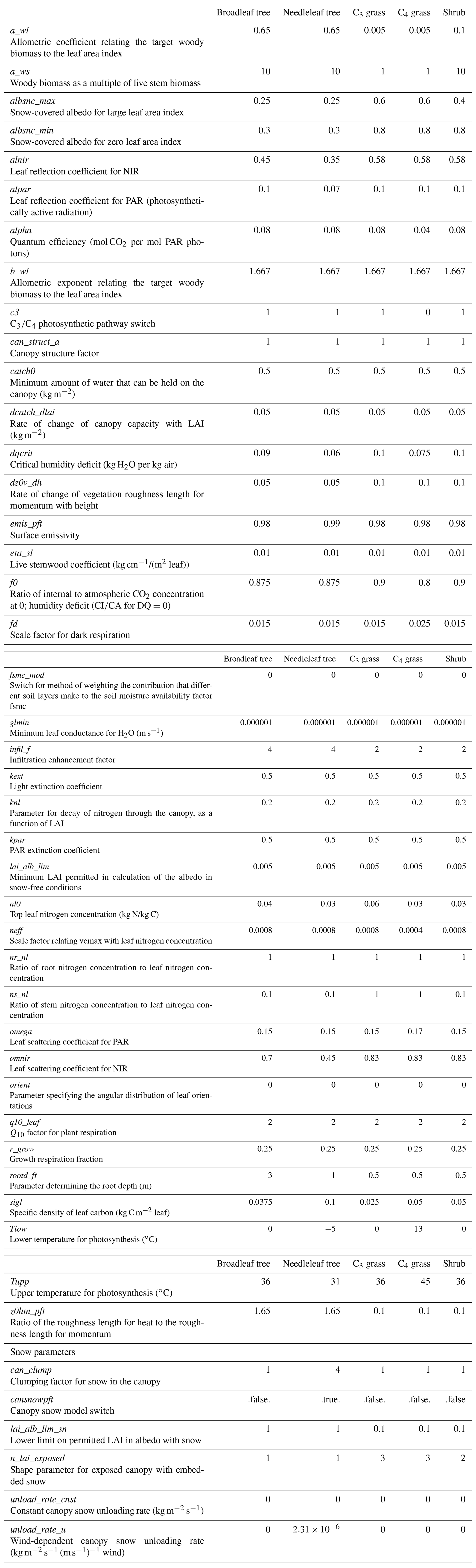
This section describes the offline JULES-GL7.0 and JULES-GL7.2 science configurations. An important difference between the offline and coupled versions is that in the coupled version JULES acts as an interface between land (including land ice), sea ice and the ocean, whilst offline only land is considered. Important parameters are listed in Tables 1 and 2, ancillaries in Table 3, and in most cases, switches are listed in the text. The full set of switch settings can be found in the Rose suites. We include the full parameter tables for the surface tiles here for clarity as the Rose suite namelists encompass all parameters in JULES, many of which are linked to particular switches and options and therefore not used in JULES-GL7. Work is progressing to simplify the Rose suite namelists using existing tools within Rose to hide unused parameters and options. The appropriate JULES documentation papers remain Best et al. (2011) and Clark et al. (2011). Where new developments are included, they are described in more detail with appropriate references herein.

Table 1 Parameters in JULES-GL7 that vary with non-vegetated surface types (note that these can be found in nvegparm).

Table 2 Parameters in JULES-GL7 that vary by PFT (note that these can be found in pftparm and snow namelists).

2.1 Surface tiling

JULES-GL7 uses a surface tiling scheme to represent subgrid heterogeneity. Within a grid box, each tile has its own surface energy budget and is coupled to a single shared soil column (Fig. 1). Each tile therefore has its own albedo, surface conductance to moisture, turbulent fluxes, ground heat flux, radiative fluxes, canopy water content, snow mass and melt, and thus surface temperature. Each tile requires its own parameter set which is given in Tables 1 (non-vegetated surface types) and 2 (vegetated surface types) and spatially explicit parameters in Table 3.

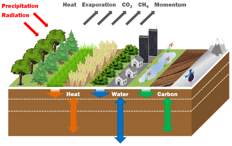
Figure 1 JULES schematic of the fluxes of stores of heat, water, carbon and momentum, and the surface tiling representation of subgrid heterogeneity.

There are nine surface tiles consisting of five plant functional types (PFTs) (broadleaf trees, needleleaf trees, C₃ grass, C₄ grass and shrubs) and four non-vegetated surface types (urban, inland water, bare soil and ice) (Fig. 2). These can coexist in the same grid box except for ice. The C₄ distinction reflects a different photosynthetic pathway with all other PFTs represented as C₃. The tile fractions are spatially varying and are read from an ancillary file. The fractions are produced by a remapping of the 17 surface types in the IGBP (Loveland and Belward, 1997) to the nine surface types in JULES. The land cover class remapping procedure is described in Table 4 of Walters et al. (2019) and the cross-walking table relating land cover classes to PFTs in Table B1.

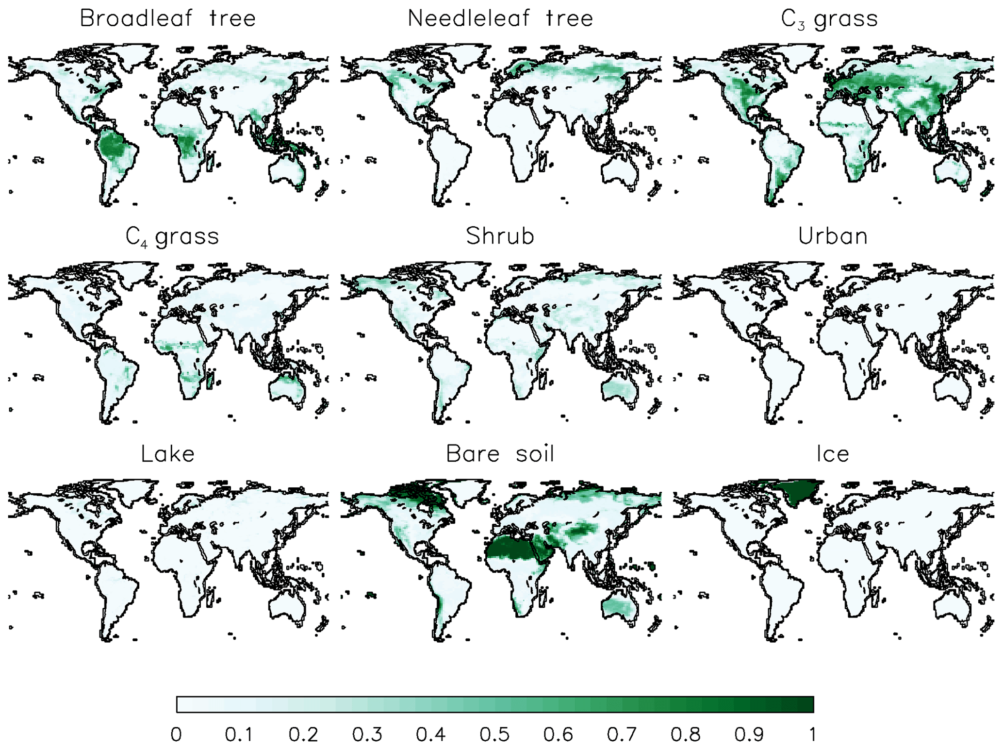
Figure 2 Surface tile fractions as used in JULES-GL7 derived from the IGBP land cover dataset (IGBP: Loveland et al., 2000).

2.1.1 Plant functional types (PFTs)

Vegetation is represented by the five plant functional types described above. In JULES-GL7, each PFT has its own energy budget including thermal heat capacity (CanMod=4), which is a function of the PFT height (Sects. “Spatial leaf area and canopy height ancillary data” and 2.3). Leaf-level stomatal conductance and photosynthesis are coupled through CO₂ diffusion with PFT-specific parameters controlling sensitivity to humidity deficit and internal to external CO₂ pressures (Cox et al., 1998 and Table 2; f0, dqcrit). This coupling implies that both the energy and carbon cycles are closely related; rising atmospheric CO₂ influences stomatal conductance and therefore the surface energy budget. This mechanism is known as physiological forcing (Betts et al., 2007; Field et al., 1995; Sellers et al., 1996). Leaf-level conductance must be scaled to the canopy level, and in JULES-GL7 this is done using a 10-layer canopy approach (CanRadMod=4). At each level, separate direct and diffuse photosynthetically available radiation (PAR) levels are calculated using the two-stream approach (Sellars, 1985) to give a profile of PAR through the canopy. From this, the leaf-level photosynthesis can be calculated using PFT-specific parameters combined with the Collatz et al. (1992, 1991) leaf biochemistry model utilising separate mechanisms for C₃ and C₄ plants (Jogireddy et al., 2006; Mercado et al., 2007). At each level, if net photosynthesis is negative or stomatal conductance is below a minimal threshold (glmin; Table 1), the stomata are closed and the stomatal conductance is set to this minimum. A further mechanism scales leaf-level conductance via photosynthesis according to the availability of soil moisture in the rooting profile. In JULES-GL7, this scalar (β) relates the rooting profile (rootd; Table 2) in each soil layer with the availability of soil moisture. β is a piecewise function that scales from 0 when soil moisture is at or below the wilting point to 1 where soil moisture is above the critical point (Eq. 12; Best et al., 2011). The root fraction weighted (fsmc_mod=0) total across soil layers value of β is used to scale photosynthesis at the leaf level. Canopy conductance is the leaf area weighted sum of leaf conductance across the 10 levels. A direct output from this setup is a diagnostic of gross primary productivity (GPP). However, as this is the non-biogeochemical configuration, the fixed GPP does alter the canopy structure.

Table 3 Ancillary information as required in the JULES-GL7.0/7.2 configurations. Required ancillary files cover parameter values that are either spatially or temporarily explicitly necessary to define the science configuration. Additional ancillaries covering grid setup and forcing are used in the experimental setup.

Spatial leaf area and canopy height ancillary data

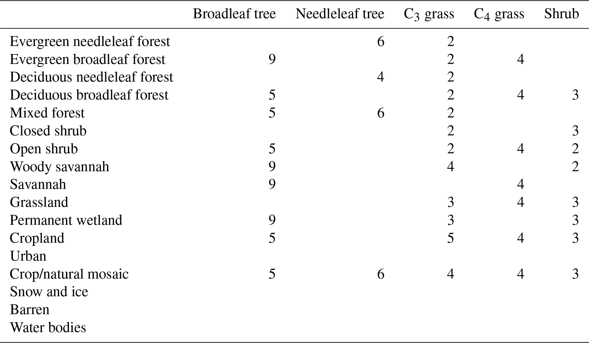
Leaf area index (LAI) is defined as the one-sided surface area of canopy leaf cover per unit area of land and is defined spatially and temporally for each vegetated surface tile in JULES-GL7. Similarly, canopy height is spatially varying per vegetated tile but fixed in time. The ancillaries are derived from satellite data processed to be consistent with the land cover and plant functional type classifications used in JULES-GL7. To do this requires decomposing a “mixed” signal from the satellite data into individual PFT contributions. This is achieved via an additional parameter, the “balanced” LAI (Lb), meaning the LAI that would be reached if the plant was in full leaf (Table B2). The combination of the mapping from land cover classes to PFTs and the balanced LAI weighting per PFT per land cover class allows the observed gridded satellite value to be decomposed into individual PFT contributions.

In JULES-GL7, monthly variations in LAI about the balanced LAI are based on a climatology for the period 2005 to 2009 derived from the MODIS LAI product (MOD15; Yang et al., 2006). The LAI value for a given PFT, land cover class and month are calculated as follows:

$$\begin{array}{}\text{(1)}& {\displaystyle }{\mathrm{LAI}}_{i,j}={\mathrm{LAI}}_{\mathrm{MODIS}}{\displaystyle \frac{\left({\mathrm{Lb}}_{i,j}{\mathit{\alpha }}_{i,j}\right)}{\sum _i\left({\mathrm{Lb}}_{i,j}{\mathit{\alpha }}_{i,j}\right)}},\end{array}$$

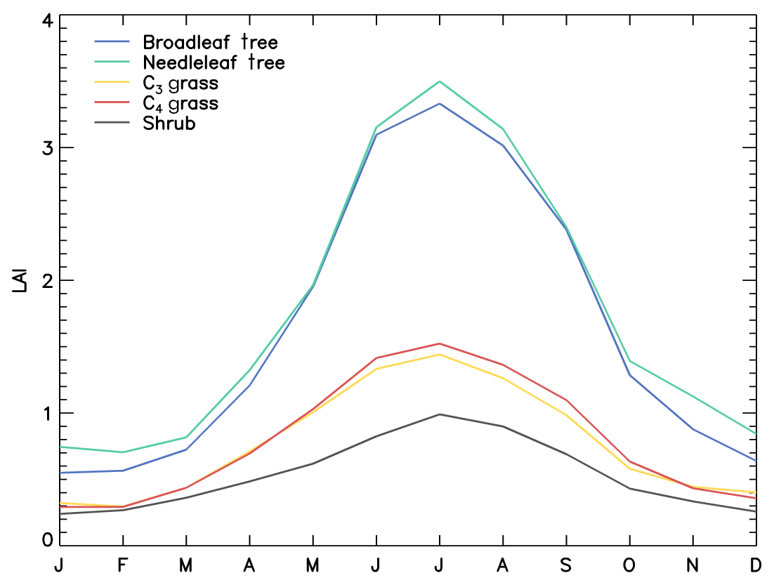
where LAI_i is the LAI for PFT class i, LAI_MODIS is the MODIS LAI value for a given month, Lb_i,j is given by the LAI lookup table (Table B2), α_i,j is the fraction of each PFT i in IGBP class j given by the lookup table in Table B1. The PFT-specific LAI (LAI_i) is accumulated for all land cover classes in a grid box for a given month. The resulting input ancillary is then internally interpolated within JULES to each model time step. The seasonally varying LAI for five PFTs for 30–60^∘ N is shown in Fig. 3. An outcome of this approach is that JULES is forced with the snow-free LAI, which explains the large winter reductions in LAI for needleleaf trees. Improving the treatment of LAI in the ancillary information is a priority development for future versions of GL.

Figure 3 Seasonal LAI for the five vegetation surface types, area averaged over 30–60^∘ N.

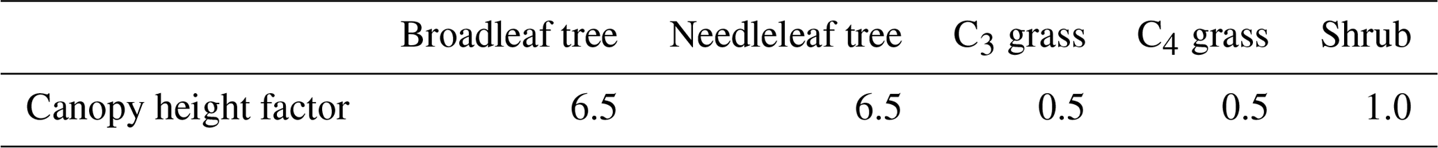
The introduced balanced LAI has the property of being allometrically related to the canopy height. Based on this allometric relationship, the canopy height (H) can be derived for each PFT in each land cover class (Jones, 1998):

$$\begin{array}{}\text{(2)}& {\displaystyle }{H}_{i,j}=h_i{\mathrm{Lb}}_{i,j}^{\frac{\mathrm{2}}{\mathrm{3}}},\end{array}$$

where h_i is a PFT-specific scalar given in Appendix B (Table B3). The PFT cover mean height (canht) is the area-weighted arithmetic mean of the land cover classes in that grid box. Canopy height (Fig. 4) is therefore based on allometric scaling of land-cover-class-dependent parameters. Improving the representation of canopy height is also a priority area for future developments.

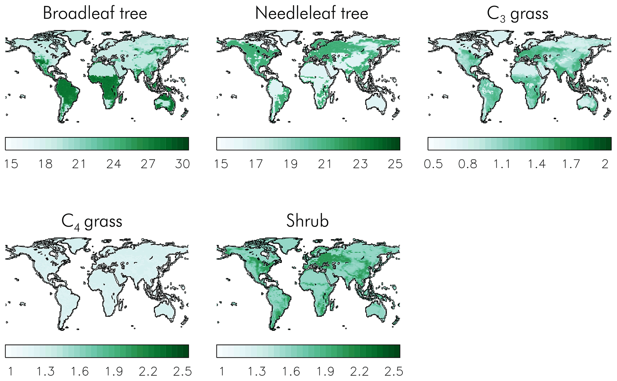
Figure 4 Canopy height (m) per PFT, as used in JULES-GL7, derived from the IGBP land cover dataset (IGBP: Global Soil Data Task, 2000).

2.1.2 Non-vegetated surface types

The four non-vegetated surface types (urban, inland water, bare soil and land ice) like the vegetated surface types are represented as tiles with separate energy balances, described using the parameters listed in Table 1. A full description of the representation of the non-vegetated surface types can be found in Best et al. (2011), and the developments after this paper have been highlighted here. After GL3.0 (Walters et al., 2011), the urban surface has been represented by the simple one-tile scheme (l_urban2t=.false.), which consists of a radiatively coupled (vf; Table 1) “urban canopy” with the thermal characteristics (ch; Table 1) of concrete (Best, 2005). The urban canopy has a capacity to hold water (catch; Table 1), and when wet, the surface moisture resistance is reduced to zero. Similar to the urban surface, lakes are represented as a radiatively coupled “inland water canopy” with the thermal characteristics of a mixed layer depth of water (≈5 m). The original representation of inland water, as a freely evaporating soil surface (ch=vf=0.0; Table 1), was shown to have incorrect seasonal and diurnal cycles for surface temperatures and therefore evaporation (Rooney and Jones, 2010). The high thermal inertia of the urban and lake tiles results in an improved diurnal cycle in surface air temperature. Bare soil or bare-ground surface types are represented as having no canopy heat capacity and a surface moisture resistance to evaporation as a function of surface soil moisture (Eq. 17, Best et al., 2011). Ice surfaces are an exception to the representation of surface heterogeneity, as only ice can exist in a grid box. This is because the subsurface is modified to represent the thermal characteristics of ice. No infiltration is allowed, and all melt is assumed to be surface runoff. The surface temperature is limited to the melting point with the residual energy balance term assumed to be melt. As such, ice surfaces do not conserve water.

The roughness lengths for inland water, bare soil and ice were updated to their current values as part of GL4.0 (Walters et al., 2014). The roughness length (z0; Table 1) for inland water was reduced to $\mathrm{1}\times {\mathrm{10}}^{-\mathrm{4}}$ m, as GL3.0 suffered from a slow bias when compared to reanalyses in the near-surface wind speed around the Great Lakes. This reduced value is more consistent with the values predicted from wind-speed-dependent parameterisations over open water (Walters et al., 2014). The roughness length for bare soil was increased to $\mathrm{1}\times {\mathrm{10}}^{-\mathrm{3}}$ m, an intermediate value between those used in GL3.0 ($\mathrm{3}\times {\mathrm{10}}^{-\mathrm{4}}$ m) and GL3.1 ($\mathrm{3.2}\times {\mathrm{10}}^{-\mathrm{3}}$ m, used in operational global NWP forecasting). Observational estimates of the roughness length of bare soil surfaces suggest large geographical variations covering this range. The ratios of the roughness lengths for heat to momentum (z0hm; Table 1) were also revised as part of GL4.0 in conjunction with the roughness length changes. From GL4.0, the urban surface has used the Best (2006) value of $\mathrm{1}\times {\mathrm{10}}^{-\mathrm{7}}$ m; for inland water, the ratio has been set to 0.25, consistent with the parameterisation for open sea; bare soil was decreased to 0.02 to address a significant underestimate of the near-surface temperature gradient over arid regions; and ice was adjusted to 0.2 to be consistent with sea ice. Prior to GL4.0, all ratios had a fixed value of 0.1. Another new capability introduced with GL4.0 was an emissivity for each surface type (emis; Table 1) based on the data of Snyder et al. (1998) and additionally for bare soil, satellite retrievals of land surface temperature from over the Sahara. Previously, these values were fixed at 0.97 regardless of surface type. The significant reduction in the bare soil emissivity improved a cold bias over the Middle Eastern deserts that was prominent in GL3.0. The description of the non-vegetated surface types in JULES-GL7 remains largely unchanged since GL4.0 (Best et al., 2011).

2.2 Radiation

Typically, stand-alone JULES is driven with downward shortwave and longwave radiative fluxes. To obtain the net fluxes that enter the surface energy budget, the surface albedo and emissivity must be calculated. The albedo varies with wavelength, although, for many natural surfaces, it is adequate to distinguish between the visible and near-infrared parts of the spectrum. In reality, the albedo is also different for direct and diffuse radiation, but a distinction is not made for every surface in GL7.

For unvegetated surfaces, single broadband albedos are used (albsnf; Table 1). The albedo of bare soil must be specified as ancillary data, but fixed values are used for the other three unvegetated tiles.

The albedo of plant canopies is calculated using the two-stream radiation scheme described by Sellers (1985). As input, this requires separate transmission (omega, omnir; Table 2) and reflection coefficients (alpar, alnir; Table 2) in the visible and near-infrared regions, respectively, for individual leaves (or shoots in the case of needleleaf trees) and the leaf area index. It returns the visible and near-infrared albedos for direct and diffuse radiation. However, the direct components are discarded and not used in GL7 for reasons of performance when coupled to the UM. When coupled to the UM, there is an option (l_albedo_obs) to scale the leaf-level characteristics to match a specified climatology of the albedo, but this is unavailable offline.

A new albedo scheme for snow-covered surfaces was introduced into GL7. This incorporates a two-stream algorithm for the snowpack. The surface is modelled as an underlying soil surface, above which there is a plant canopy that is gradually buried as snow accumulates. The canopy is therefore modelled as a lower snow layer and an upper layer of exposed vegetation that will be absent if the snow is deep enough. The scheme makes explicit use of the canopy height. If canopy snow is allowed on the tile, there will also be a layer of snow on the canopy that is treated using the same two-stream scheme. Additional parameters (can_clump, n_lai_exposed) represent the vertical distribution of leaf area density and the clumping of snow on the canopy. However, the values adopted in GL7 have been tuned to work with the existing ancillaries of canopy height which exhibit unrealistically limited spatial variability. Previously, a hard-wired lower limit of 0.5 had been imposed on the LAI in the calculation of the albedo. In GL7, this has been removed and replaced with separate limits for snow and snow-free conditions. In snow-free conditions, the nominal lower limit has been set to 0.005, while in the presence of snow a limit of 1.0 is imposed for trees and a limit of 0.1 in the case of short vegetation (Table 2). Infrared emissivities are specified as single broadband values for each surface type (Tables 1 and 2).

2.2.1 Diffuse radiation

GL7 assumes that PAR is half of the total downwelling shortwave. The PAR as seen in the plant physiology is entirely direct, which results in a lower penetration of PAR into the canopy and reduced photosynthesis at the subcanopy level. For GL7.2, we introduce a constant global mean diffuse fraction of 0.4, based on output from the SOCRATES radiative transfer scheme (Edwards and Slingo, 1996; Manners et al., 2018). This has the impact of increasing light penetration into the canopy and therefore increasing GPP. To further improve GPP, we updated the canopy radiation model (can_rad_mod, changed from 4 to 6). Like can_rad_mod$=\mathrm{5},\mathrm{6}$ introduces sunfleck penetration through the canopy ($\text{fsun}=\exp (-\frac{k_b}{\cos z}\mathrm{LAI});k_b$ constant value of 0.5) which increases the light within the canopy particularly for high solar zenith angles. Furthermore, can_rad_mod=6 introduces a new nitrogen profile through the canopy following exp (−k_nlLAI), where k_nl is a PFT constant of 0.2 (Table 2). This has the effect of increasing potential GPP in canopies with low LAI (<5) and decreasing at high LAI (>5). GL7.2 is consequently a physically more realistic configuration of JULES. The changes to canopy radiation do not affect the simulated albedo, as in the current setup the albedo is only calculated for direct radiation. GL7.0 and 7.2 will therefore have the same albedo, but the way light interacts with the canopy differs and therefore affects the exchange of moisture and carbon.

2.3 Surface exchange

The representation of the surface energy budget in JULES is described by Best et al. (2011). The scheme includes a surface heat capacity. Atmospheric resistances are calculated using standard Monin–Obukhov surface layer similarity theory, using the stability functions of Beljaars and Holtslag (1991). Evaporation from bare soil and water on the canopy and transpiration through the plant canopy contribute to the latent heat fluxes. In the case of needleleaf trees, snow on and beneath the canopy is treated separately (can_mod=4).

2.4 Soil hydrology and thermodynamics

Soil processes are represented using a four-layer scheme for the heat and water fluxes with hydraulic relationships taken from Van Genuchten (1980). The four layers (0.1, 0.25, 0.65 and 2 m) are chosen to capture diurnal, seasonal and multiannual variability in soil moisture and heat fluxes. The JULES-GL7 soil parameter values are based in part on those developed for the MOSES model by Dharssi et al. (2009) and Cox et al. (1999), and are read from an ancillary. There is an additional deep layer with impeded drainage to represent shallow groundwater, thus enabling a saturated zone and water table to form. The subgrid-scale soil moisture heterogeneity model is driven by the statistical distribution of topography within the grid box and is based on a TOPMODEL-type approach (Gedney and Cox, 2003). The baseflow out of the model is dependent on the predicted grid box mean water table, while surface saturation and wetland fractions are dependent on the distribution of water table depth within the grid box. The scheme uses the Marthews et al. (2015) topographic index dataset at 15 arcsec resolution, which in turn is derived from HydroSHEDS (Lehner et al., 2006). The soil and hydrological ancillaries required are listed in Table 3.

2.5 Snow

A major difference between GL7 and earlier GL configurations is the activation of the multilayer snow scheme in JULES that is described by Best et al. (2011). This replaces the previous so-called zero-layer scheme in which a single thermal store was used for snow and the first soil level, and an insulating factor was applied to represent the lower thermal conductivity of snow. The zero-layer scheme included no representation of the evolution of the snowpack. Compared to the version described in Best et al. (2011), a number of enhancements have been introduced into the multilayer scheme in order to better to represent the thermal state of the snow surface and atmospheric boundary layer when coupled to the UM. The changes are noted in the following description and parameter values in Table 2.

In the multilayer scheme, the snowpack is divided into a number of layers that are added or removed as the snowpack grows or shrinks. A maximum of three layers is imposed in GL7. In a deep snowpack, the top layer will be 0.04 m thick, the second 0.12 m thick, while the lowest layer will contain the remainder of the snowpack. Very thin layers of snow (less than 0.04 m deep) are still represented using the zero-layer scheme for reasons of numerical stability. The thickness, frozen and liquid water contents, temperature and grain size of each layer are prognostics of the scheme. New snow is added to the top of the snowpack and compaction by the overburden is included. Following these operations, the snowpack is relayered to the specified thickness.

The density of fresh snow has been set to 109 kg m⁻², following the scheme adopted in the CROCUS model (Vionnet et al., 2012), but omitting the wind speed and temperature-dependent factors. The conductivity of snow was originally calculated using the parameterisation of Yen (1981), but this has been replaced with the scheme proposed by Calonne et al. (2011). This gives higher conductivities in snow of low density, thereby strengthening the coupling between the snowpack and the boundary layer.

Again, with a view towards improving the coupling between the atmosphere and the snowpack, the parameterisation of equi-temperature metamorphism described by Dutra et al. (2010) has been introduced. This accelerates the rate of densification of fresh snow and is important in reducing cold biases that would otherwise result.

In the original scheme, when the canopy snow model was selected, unloading of snow from the canopy occurred only when it was melting. In GL7, unloading (unload_rate_u; Table 2) is also permitted at colder temperatures, and the timescale is set to 1∕(unload_rate_u *wind velocity at 10 m), which is tuned to give an unloading timescale of 2 d in the Canadian boreal forest in winter (MacKay and Bartlett, 2006) for the average 10 m wind speed predicted in the UM. Note that a separate canopy is currently used only for the needleleaf tile.

Unlike the original scheme, where it simply bypassed the snowpack, rainwater is now allowed to infiltrate. Below a canopy, this infiltrating water includes melting from the canopy.

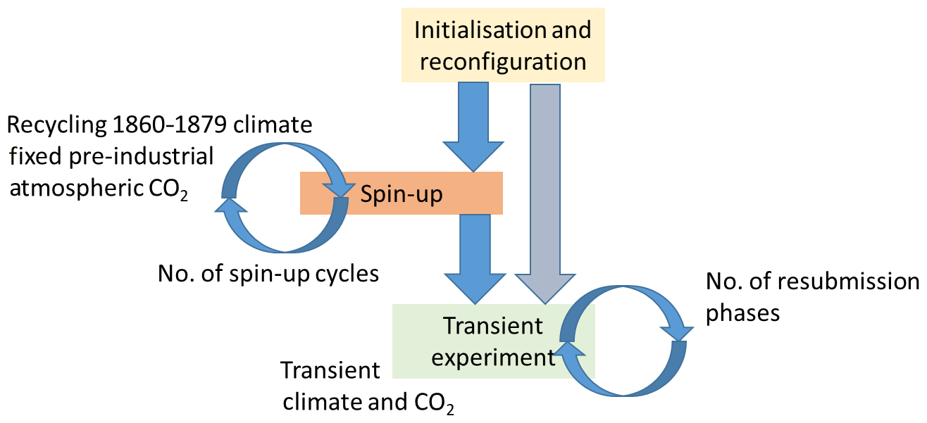
Figure 5 Suite control used to initialise, spin up and perform a full transient experiment with JULES-GL7.

2.6 Coupled versus uncoupled differences

JULES has been developed in more than one modelling environment, i.e. stand-alone and coupled with the UM, and consequently some science options are not available under all environments. This could be because certain science options only make sense in a coupled environment or the converse may be true. This is not true for all options and in some cases the options have only been implemented in one environment and require additional coding to make it available to others. Other differences arise out of the method of coupling the available driving data. When coupled, the surface meteorological state is solved interactively, whereas offline this is provided either from observation or reanalysis products. One important difference concerning the treatment of radiation (jules_radiation) is that when coupled separate radiative fluxes of NIR and PAR are available from the radiation scheme, offline, typically only broadband shortwave is available, and it is assumed this can be split 50:50 between NIR and PAR. Furthermore, when coupled, snow-free albedos on each surface type are nudged towards an observed climatological mean from an ancillary (l_albedo_obs = .true.). This approach maintains sensible differences between surface types and allows spatial differences in albedo properties to be captured, while agreeing well with observations. However, in turn, this has some limitations and as such it is not suitable for climate change experiments that include a change in land cover. It is therefore not compatible with the dynamic vegetation and land-use models as those used in the interactive carbon cycle option and thus is not implemented in the offline JULES-GL7 configuration. Another subtle difference concerning the treatment of radiation is the calculation of the solar zenith angle. When coupled, the SOCRATES radiative transfer scheme calculates this, whereas in stand-alone JULES, the solar zenith angle calculation needs to be explicitly turned on using l_cosz=.true. to be equivalent. When using JULES-GL7 therefore with site data, care should be taken to ensure that the model and forcing data are in Coordinated Universal Time (UTC), as time is used in the calculation of solar zenith angle.

There are several differences in the treatment of the JULES surface exchange (jules_surface), as this is the interface between the surface and either the driving model or the driving data. Orographic form drag (formdrag=0stand-alone, 1 coupled), for example, cannot be used in the stand-alone configuration, as the necessary ancillary data are not available to stand alone. In any case, it may not make scientific sense to include this, as the orographic drag may be implicit in the driving data either from observations or from model-generated driving data. The method of discretisation in the surface layer is another difference between the two environments which affects how the driving data are interpreted. The driving data, when in stand-alone configuration, are most likely to be at a specific level (i_modiscopt=0) rather than a vertical average as they are when coupled (i_modiscopt=1). Also in the coupled model, a parameterisation of transitional decoupling in very light winds is included in the calculation of the 1.5 m temperature (iscrntdiag=2); however, in stand-alone configuration, the surface is driven by the temperature at 1.5 m and is therefore not a diagnostic. It is not recommended that the surface is driven with a decoupled variable, as this scenario has not been properly tested and should instead be iscrntdiag =0. Finally, concerning the surface exchange, the coupled model includes the effects of both boundary layer and deep convective gustiness (isrfexcnvgust =1); however, this is not appropriate in stand-alone mode, and therefore isrfexcnvgust =0. When driving stand-alone JULES with observations at a high-enough frequency, the gusts would be implicit in the observational data; and in the case of driving JULES with a longer-term average, where there may be a gust contribution, the relevant information is not accessible.

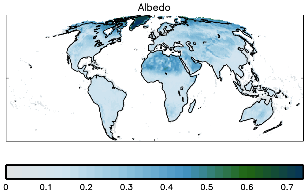
Figure 6 Surface albedo 2000–2005 benchmark derived from MODIS (De Kauwe et al., 2011), as generated by ILAMB (Collier et al., 2018).

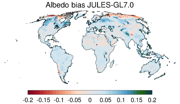
Figure 7 Albedo bias simulated by GL7.0 relative to the MODIS benchmark. Means over 2000–2005 are shown. Biases are calculated as the difference between the model and observations.

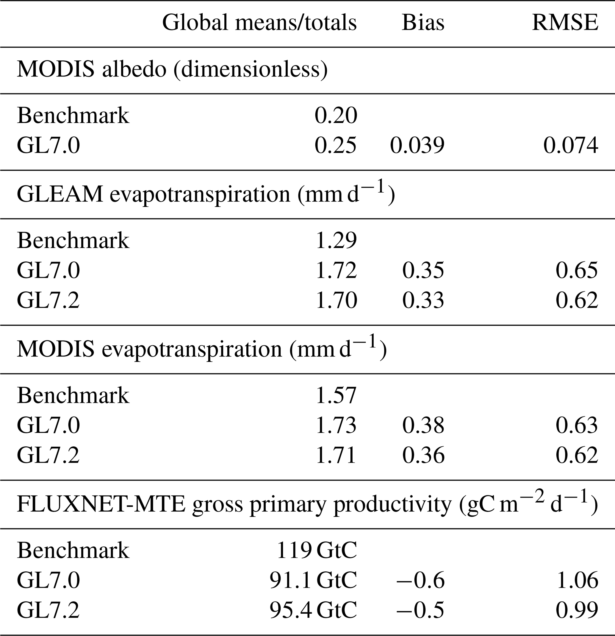
Table 4 Tabulated measures of model performance against benchmarks. Global means and totals are calculated on the native grid of the observational and model grids accounting for fractional land coverage in the totals and weighting for irregular grid box sizes. Biases and root mean square errors (RMSEs) are calculated by regridding the observational data to the coarser model grid and calculating metrics where the observational and model data intersect.

3 JULES-GL7 experimental setup and suite control

The science configuration consists of a defined set of parameters and switches that can be used in conjunction with an experimental setup. The experimental setup differs from the configuration, as it describes the conditions under which the configuration is applied. For example, in this case, the setup is a global historical experiment, but it could also be a future climate scenario, driven by alternative historical forcing or at multiple locations, such as FLUXNET sites, where more detailed evaluation data are available (e.g. Harper et al., 2016). The experiment in the suite provided is a global historical run from pre-industrial (1860) to the present day (2014) including rising atmospheric CO₂ but fixed land cover. This is a standard historical experimental setup as used in the Global Carbon Project (Le Quéré et al., 2015). The climate data (Climate Research Unit – National Centers for Environmental Prediction; CRU-NCEP v7) consist of 6-hourly NCEP data corrected to CRU climatology and observations updated to 2014 (CRU TS3.23; Harris et al., 2014). The original data were provided on a $\mathrm{0.5}{}^{\circ }\times \mathrm{0.5}{}^{\circ }$ grid and subsequently regridded to a coarser resolution for consistency with the standard resolution climate experiments for CMIP6 using HadGEM3-GC3.1 at $\mathrm{1.875}{}^{\circ }\times \mathrm{1.25}{}^{\circ }$. The forcing data include both gridded observations of climate and global atmospheric CO₂, which change over time (Dlugokencky and Tans, 2015). However, the CRU-NCEP data only start in 1901. To begin the experiments in 1860, a time when atmospheric CO₂ was relatively stable, requires the years 1901–1920 to be replicated between 1860 and 1900, thus assuming no effect of climate change between 1860 and 1901. CRU-NCEP uses a 365 d calendar, so no leap years are included. Furthermore, CRU-NCEP is a land-only dataset including Greenland but excluding Antarctica. At the coarser resolution, a grid box may only be partially land covered. JULES works on the land-only fraction of the grid box. It is therefore important when making global means or averages that both the land fraction of a grid box as well as the grid box area are considered. An important provided ancillary is therefore the land fraction (Table 3).

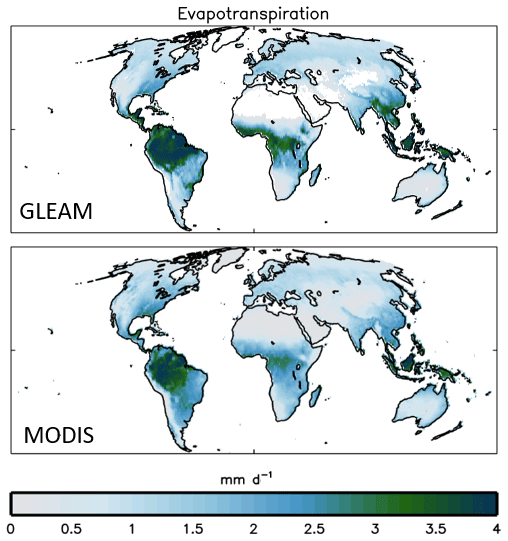
Figure 8 Surface evapotranspiration benchmarks derived from GLEAM (Miralles et al., 2011) and MODIS (Mu et al., 2013), as generated by ILAMB (Collier et al., 2018), covering 1980–2011 and 2000–2013, respectively.

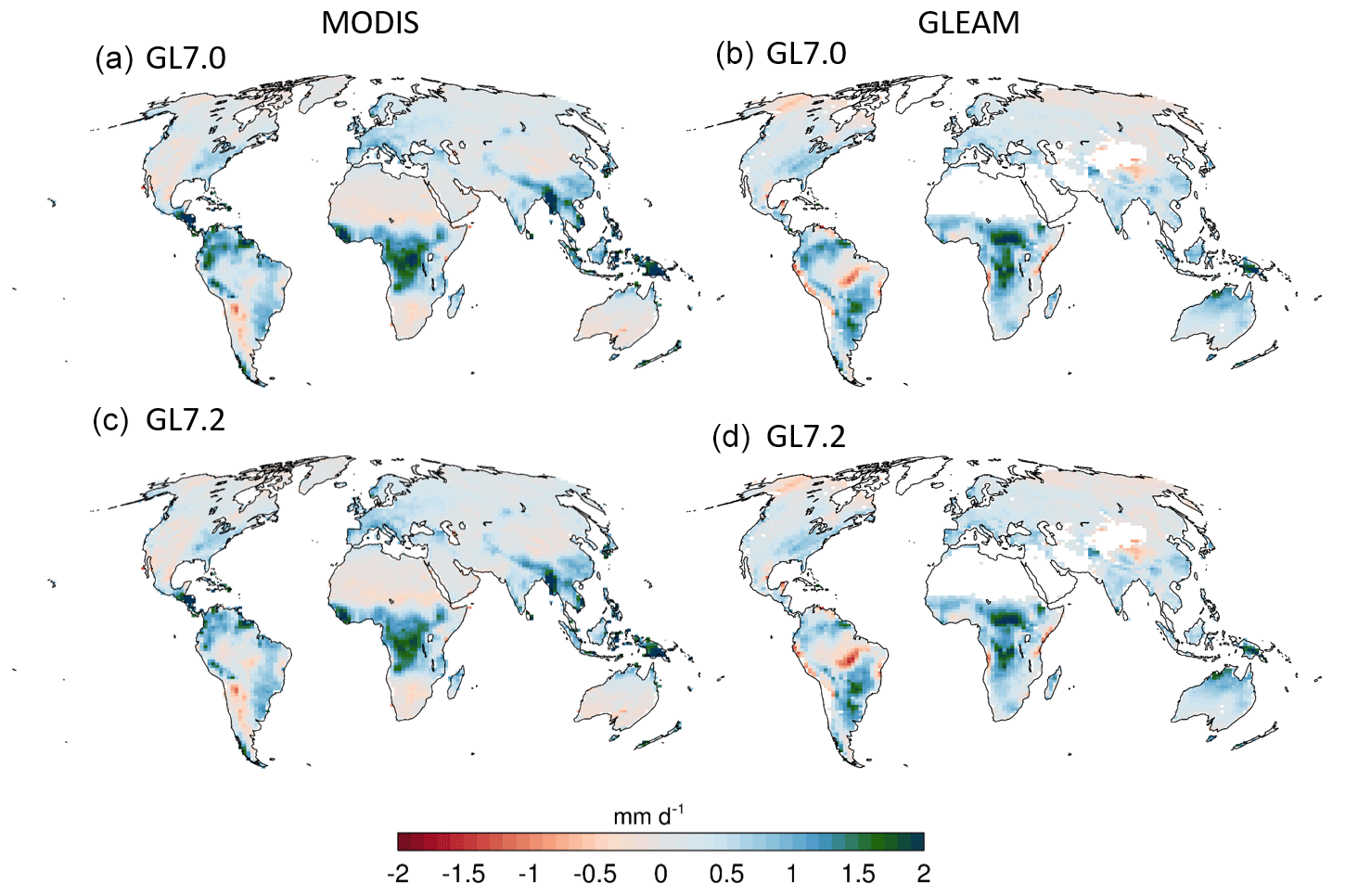
Figure 9 Evapotranspiration biases simulated by GL7.0 (a, b) and GL7.2 (c, d) for MODIS (a, c) and GLEAM (b, d) benchmarks. MODIS means are for 2000–2013 and GLEAM for 1980–2011. Biases are calculated as the difference between the model and observations.

The suite, as provided, includes a standardised suite control approach to manage both the necessary stages of initialising and running an experiment as well as scheduling resources and time slots on the supercomputer. This is shown graphically in Fig. 5. The suite is set up to run three separate instances of JULES. The first initialises and reconfigures an initial start condition. The second starts from the reconfigured start condition and spins up the states of snow, soil moisture and temperatures by cycling over 1860–1879 climate using fixed pre-industrial CO₂. This is optional according to whether the initial state is already spun-up and is controlled by a switch (l_spinup). Setting this switch to false bypasses the spinup entirely. The number of cycles required and the period to loop over can also be set. Each new cycle of spinup is submitted as a new job taking the initial conditions from the end of the previous cycle. The final task is to perform the transient experiment taking either initial conditions from the reconfiguration step or the final spinup cycle. These settings are all available under Runtime Configuration and Runtime Configuration > Spinup Options. The transient run makes uses of varying climate and atmospheric CO₂. As a standard, the transient experiment has a 10-year cycle interval to allow a complete cycle to complete within the time limits on the supercomputer. It is worth noting that JULES vn5.3 is unable to perform full bit-comparable restarts. This means the model prognostics at the end of one submission differ slightly from those used at the start of the next. The exact state at the end of the transient run will therefore be dependent on the number of spinup and transient cycles used.

Figure 10 GPP (1982–2008) benchmark derived from FLUXNET-MTE (Jung et al., 2010) as generated by ILAMB (Collier et al., 2018).

4 JULES-GL7 evaluation

In this section, we evaluate the CRU-NCEPv7 historical experimental setup of the JULES-GL7 model configuration. We follow the approach of the International Land Model Benchmarking (ILAMB) project tool (Collier et al., 2018) to compare model simulations against observational data. However, due to technical limitations, we are unable to use the full benchmarking range that ILAMB includes. Here, we assess model performance against three key metrics covering surface energy balance, hydrology and vegetation productivity. The metrics are annual mean albedo, evapotranspiration and gross primary productivity, and they are benchmarked against observationally based datasets available in ILAMB. The aim here is not to perform a full analysis of model skill but to establish a few important benchmarks against which model developments can be compared and evaluated. In time, it is planned that the standardised JULES suite will be fully compatible with ILAMB, allowing for a full model evaluation and benchmarking to be completed in a straightforward and standardised way. Furthermore, caution should be taken in benchmarking a model using a single forcing dataset. As part of the Land Surface, Snow and Soil Moisture Model Intercomparison Project (LS3MIP; van den Hurk et al., 2016), this configuration will be setup with GSWP3 forcing data, which in time will be made available to the community. A second dataset will allow sampling of model uncertainty arising from forcing data variation.

Surface albedo is simulated in the model as described in Sect. 2.2. Globally, the observed land surface albedo is generally higher in snow-covered regions and deserts, as shown in the MODIS satellite data (Fig. 6). As noted in Sect. 2.2.1, the simulated albedo in JULES-GL7.0 and 7.2 are exactly the same, despite having different canopy radiation options, as the differences only affect light availability for photosynthesis. Overall, we find the model is too bright with a globally positive bias (Table 4). However, Fig. 7 shows that the bias is spatially variable, with the largest biases (both positive and negative) found in the high latitudes and other snow-covered regions. In general, in this experimental setup, we find the surface is too bright in regions of boreal forests and too dark across the far north in the tundra regions.

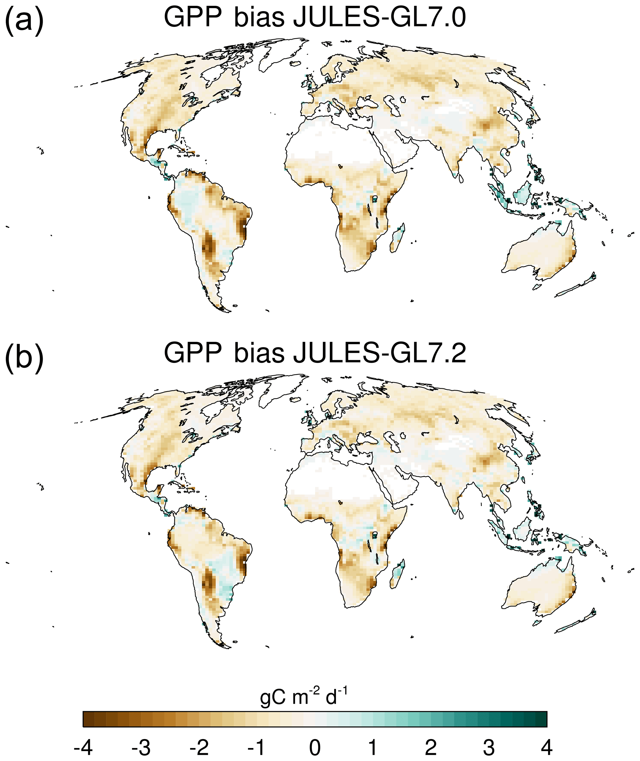
Figure 11 GPP biases simulated by GL7.0 (a) and GL7.2 (b) against the FLUXNET-MTE dataset. Means are for 1982–2008. Biases are calculated as the difference between the model and observations.

Evapotranspiration is benchmarked against two observational products: GLEAM (Miralles et al., 2011) and MODIS (Mu et al., 2013). There is uncertainty in the two datasets, with large differences in the magnitude of evapotranspiration particularly over the tropical regions (Fig. 8). Both GL7.0 and 7.2 have large positive biases over much of the world, and these are strongest over the tropics (up to 2 mm d⁻¹; Fig. 9). However, the exact location of the largest biases differs between MODIS and GLEAM. GLEAM suggests a dipole pattern over central Africa, while MODIS has a centralised positive bias, implying there is a degree of observational uncertainty that needs to be accounted for. Overall, the biases are slightly reduced in GL7.2 (Table 4).

Although GL7 is mainly intended for studying the exchange of momentum, heat and water, the configuration also underpins the carbon cycle configuration, and photosynthesis is strongly linked to evapotranspiration through the stomatal conductance model. It is therefore worth benchmarking the model's ability to simulate GPP. Here, we compare simulated GPP against the Fluxnet-MTE product (Fig. 10; Jung et al., 2010). Figure 11 shows that GL7.0 and 7.2 correctly predict that GPP is highest in tropical forests and low in arid areas, but there is a substantial negative bias in most biomes, with the exception of tropical forests. GL7.2 is an improvement over GL7.0, with a global total GPP of 95.4 GtC compared with 91.1 GtC in GL7.0. However, this is substantially lower than the 119 GtC in the reference dataset.

5 Summary

JULES-GL7.0 is the stand-alone version of the land surface configuration underpinning the HadGEM3-GC3.1 climate model that is being run as part of the CMIP6 round of global climate modelling experiments. It is a comprehensive model simulating the exchange of heat, water and momentum developed as part of the coupled climate model and extracted here for use by the community.

It has been shown that both JULES-GL7.0 and JULES-GL7.2 can capture the large-scale features of surface albedo, evapotranspiration and GPP; however, there are substantial biases that future updates to the configuration should attempt to reduce. There is also substantial uncertainty in observational evaluation datasets and the forcing for driving the model (Collier et al., 2018), which remains to be accounted for. Caution therefore needs to be taken to avoid overfitting the model to just a few datasets without a full appreciation of the uncertainties involved. In time, we plan to add additional forcing datasets to the standard configuration and the ability to benchmark against the full capability available in ILAMB.

This configuration and the ability to run the model are provided to the land surface modelling community to promote community engagement in the advancement of land surface science whether through application in their individual study, for use in model intercomparison studies such as LS3MIP (van den Hurk et al., 2016) or to promote community science developments progressing onto the main JULES trunk and into the major science configurations that underpin weather and climate forecasting in the UK.

Appendix A: Running JULES-GL7

This section describes how to access and run the JULES-GL7.0 and JULES-GL7.2 suites provided in JULES version 5.3. It is recommended that the latest version is used, which is available from https://code.metoffice.gov.uk/trac/jules/wiki/JulesConfigurations (last access: 31 January 2020) (login required), in order to benefit from bug fixes, ease of testing and implementing developments, which can only take place at the head of the JULES code trunk.

A1 Compute platform setup

The JULES-GL7.0 and JULES-GL7.2 configurations are available as Rose suites at https://code.metoffice.gov.uk/trac/roses-u/browser/b/b/3/1/6/trunk (last access: 31 January 2020) and https://code.metoffice.gov.uk/trac/roses-u/browser/b/b/5/4/3/trunk (last access: 31 January 2020), respectively. Note that access will be required to the Met Office Science Repository Service (https://code.metoffice.gov.uk/trac/home, last access: 31 January 2020) and is available to those who have signed the JULES user agreement. JULES is freely available for non-commercial research use, as set out in the JULES user terms and conditions (http://jules-lsm.github.io/access_req/JULES_Licence.pdf, last access: 31 January 2020). The easiest way to access the repository is by completing the online form here: http://jules-lsm.github.io/access_req/JULES_access.html (last access: 31 January 2020).

The suite is configured to run on both the Met Office CRAY XC40 or the JASMIN (http://www.jasmin.ac.uk/, last access: 31 January 2020) platform provided by the Science and Technology Facilities Council UK. For non-Met Office collaborators, JASMIN is the most suitable platform for running JULES simulations. JASMIN access is available for all UK-based researchers who consider themselves part of the NERC (https://nerc.ukri.org/, last access: 31 January 2020) community. JASMIN is also available for non-UK based researchers who are interested in JULES. Once you have access to JASMIN, you will need to request access to the JULES group workspace (/group_workspaces/jasmin2/jules), which can be done here: https://accounts.jasmin.ac.uk/services/group_workspaces/jules/ (last access: 31 January 2020). Met Office CRAY XC40 users will need access to the xcel00 and/or xcef00 machines.

Installing the suite requires access to the Met Office suite and code management tools available on both JASMIN and the Met Office Linux estate. To access the tools, please follow the guidelines in Sect. A5 of the Appendix. Once you have access to the necessary compute platforms, repository and tools, you are ready to start your run.

The suite is designed for ease of use, to enable the maximum number of users to access it. The suite is configured to extract the code from the repository, build on the appropriate platform, sourcing appropriate libraries and then run using the appropriate forcing and ancillaries. Most users should be able to set a standard run going in just a few steps.

A2 Setting up the model configuration

The standard JULES-GL7.0 (JULES-GL7.2) suite, u-bb316, (u-bb543) has been configured to minimise the steps necessary to be able to run the standard configuration; however, a few important steps and checks remain. It is assumed that a JASMIN user has logged into the jasmin-cylc node and a Met Office user is accessing CRAY via a Linux desktop.

1. Create a new suite:
   

   rosie copy u-bb316
   

   This will create a new suite of your own in which changes can be made and tracked using the Met Office Science Repository Service. Remember to commit any changes back to the repository with fcm commit. Rosie copy u-bb316 results in a new suite with a similar id in alphanumeric order, e.g. u-ab123. You should replace u-ab123 with your suite id in the following commands.

2. The rosie copy command will create a local copy of the new suite in the ∼/roses directory. You can change directory to this suite.

   Once the suite is installed, you can use the Rose GUI editor to check the suite setup. There are a number of platform-specific aspects to be checked. To open the GUI, the following is necessary:
   

   rose edit -C ∼/roses/u-ab123/
   

   • a.

     Build options > JULES_FCM – this variable points to the location of the code to be compiled. In the standard case, this should point to the trunk; however, this could equally point to a branch to test a new development. An important point to note is that the CRAY uses an internal “mirror” copy of the repository held in the cloud. This avoids downtime when the repository is unavailable. This is indicated by an “m” in the repository shortcuts. This should be fcm:jules.xm and fcm:jules.x on CRAY and JASMIN, respectively. This is handled in the background by the Cylc control system; however, failure to set this correctly will result in a build failure.

   • b.

     Platform-specific > build and run mode – this radar button is used to set up the platform-specific build and installation. This should be Met Office-cray-xc40 and Jasmin-Lotus on the CRAY and JASMIN platforms, respectively.

   • c.

     Runtime configuration > MPI_NUM_TASKS – up to 16 MPI tasks are available on JASMIN. More are available on the CRAY for faster runtime. Overall, 16 MPI tasks is a recommended setup. However, 18 MPI tasks (with two OpenMPs; OMPs) make a fuller use of a single Broadwell node on the CRAY.

   • d.

     Runtime configuration > OMP_NUM_TASKS – more recently releases of JULES support more OpenMP threads. A suitable number of tasks is two.

   The suite is now installed and ready to run. On the CRAY platform, the submission can be made from the local machine. On JASMIN, it is recommended to use the Cylc workflow machine jasmin-cylc. The suite can be submitted to the scheduler.
   

   rose suite-run -C ∼/roses/u-ab123/
   

3. Assuming the suite submits correctly, the next step is to monitor progress. Met Office and JASMIN users will automatically see the suite control GUI. However, the suite can be monitored by one of the two following options:
   cylc scan --c  will show the state of running suites.
   tail -f ∼/cylc-run/u-ab123/log/suite/ log will print to screen the current status of u-ab123.

4. The output from the suite is automatically written to a directory:

   • a.

     $DATADIR/jules_output/u-ab123 on CRAY;

   • b.

     /work/scratch/$USER/u-ab123 on JASMIN.

   Note that the scratch workspace on JASMIN is not for permanent storage of model output.

A3 Making changes to model configuration

The purpose of making a standard science configuration and experimental setup available is not so users can reproduce the same results but to encourage further development and testing, whether that involves new and novel diagnostics and evaluation or new processes and ancillary information. This should be done relative to the “benchmark” standard configuration and experimental setup. To modify the configurations, users should copy the standard suite as above and switch the code base to point to the user's branch and revision number. Any new parameters and switches can then be added to the app configuration file – this can be done through the GUI or by editing the configuration file directly (∼/roses/u-ab123/app/rose-suite.conf). Note that the model code needs to be consistent with the setup in the app. Any modifications to the suite should be committed and documented on a JULES ticket similar to the one documenting the JULES-GL7 release (https://code.metoffice.gov.uk/trac/jules/ticket/837, last access: 31 January 2020).

Model developers should use the suite and information presented here in combination with the JULES technical documentation found in Best et al. (2011) and Clark et al. (2011).

A4 Inter-version compatibility

The JULES-GL7 model configurations are independent of the code release, as it is a requirement of any modification to the JULES code base that the major configurations are scientifically reproducible between code versions. This is not exactly the same as them being reproducible to the bit level, as some changes are permitted; for instance, changing the order of a do loop can have benefits for runtime but lead to changes at the bit level. From a user perspective, the differences between model releases should be pragmatically indistinguishable. It is intended that the JULES-GL7 configurations will be made available at each model release, and the latest release is preferable if undertaking configuration development. Users of the configuration may find benefits in the latest version through technical improvements to suite control tools including user interfaces and code optimisation reducing runtime. It is therefore preferable to use the latest available configuration. At some point, when a configuration is deemed superseded, the guarantee of backwards compatibility will be dropped and code modules may be removed from the code base and no longer supported.

A5 Setting up the JASMIN work environment

The following assumes you have access to JASMIN as outlined in Sect. 5. This section outlines the necessary steps to set up the necessary work environment.

On jasmin-cylc, edit your ∼/.bash_profile file:

# Get the aliases and functions

if [ -f ~/.bashrc ]; then
. ~/.bashrc

fi

# User specific environment and startup
 programs

export PATH=$PATH:$HOME/bin
HOST=$(hostname)

if [[ $HOST = "jasmin-sci2.ceda.ac.uk" ||
 $HOST = "jasmin-cylc.ceda.ac.uk" || r $HOST
  = "jasmin-sci1.ceda.ac.uk" ]]; then
  # Rose/cylc on jasmin-sci & Lotus nodes
  export PATH=$PATH:/apps/contrib/metomi/bin
fi

On jasmin-cylc, edit your ∼/.bashrc file at the top:

# Provide access to FCM, Rose and Cylc
PATH=$PATH:/apps/contrib/metomi/bin

# Ensure .bashrc is sourced in login shells
# (only add this if it is not already done
  in your .bash\_profile)
[[ -f ~/.bashrc ]] && . ~/.bashrc

At the bottom,

[[ $- != *i* ]] && return # Stop here
 if not running interactively
[[ $(hostname) = "jasmin-cylc.ceda.ac.uk" ]]
 && . mosrs-setup-gpg-agent
# Enable bash completion for Rose commands
[[ -f /apps/contrib/metomi/rose/etc/rose-
 bash-completion ]] && .
/apps/contrib/metomi/rose/etc/rose-bash
-completion

Now, whenever logging in to jasmin-cylc, you should be prompted for your Met Office Science Repository Service password.

A further setup for JASMIN and MOSRS requires an update to your ∼/.subversion/servers file. Please add the following and do not forget to give the corresponding username (change myusername to your MOSRS-username).

[groups]
metofficesharedrepos = code*.metoffice.gov.uk

[metofficesharedrepos]
# Specify your Science Repository Service
 user name here
username = myusername
store-plaintext-passwords = no

In the ∼/.subversion/config file, comment any lines starting with

#password-stores =

Create the following configuration file ∼/.metomi/fcm/keyword.cfg and add the following lines:

location{ primary, type:svn}[jules.x]=
 https://code.metoffice.gov.uk/svn/jules/main
browser.loc-tmpl[jules.x]=https://code.
 metoffice.gov.uk/trac/{1}/intertrac/source:
 /{2}{3}browser.comp-pat[jules.x]=(?msx-i:
 \A // [^/]+ /svn/ ([^/]+) /*(.*) \z)

location{primary, type:svn}[jules\_doc.x]=
 https://code.metoffice.gov.uk/svn/jules/doc
browser.loc-tmpl[jules\_doc.x]=https://code.
 metoffice.gov.uk/trac/{1}/intertrac/source:
 /{2}{3}browser.comp-pat[jules\_doc.x]=
 (?msx-i:\A // [^/]+ /svn/ ([^/]+) /*(.*) \z)

Add the following lines on the ∼/.metomi/rose.conf file if missing (change myusername to your MOSRS-username):

[rosie-id]
prefix-default=u
prefix-location.u=https://code.metoffice.
 gov.uk/svn/roses-u
prefix-username.u=myusername
#username is all in lower case
prefix-ws.u=https://code.metoffice.gov.uk
 /rosie/u

[rose-stem]
automatic-options=SITE=jasmin

This can be checked by running

rose config

Appendix B: Plant functional type, leaf area index and canopy height cross-walking tables

Table B1 PFT fraction lookup table for vegetated PFTs only. BLT indicates broadleaf tree; NLT indicates needleleaf tree. These lookup tables are used in conjunction with Eqs. (1) and (2).

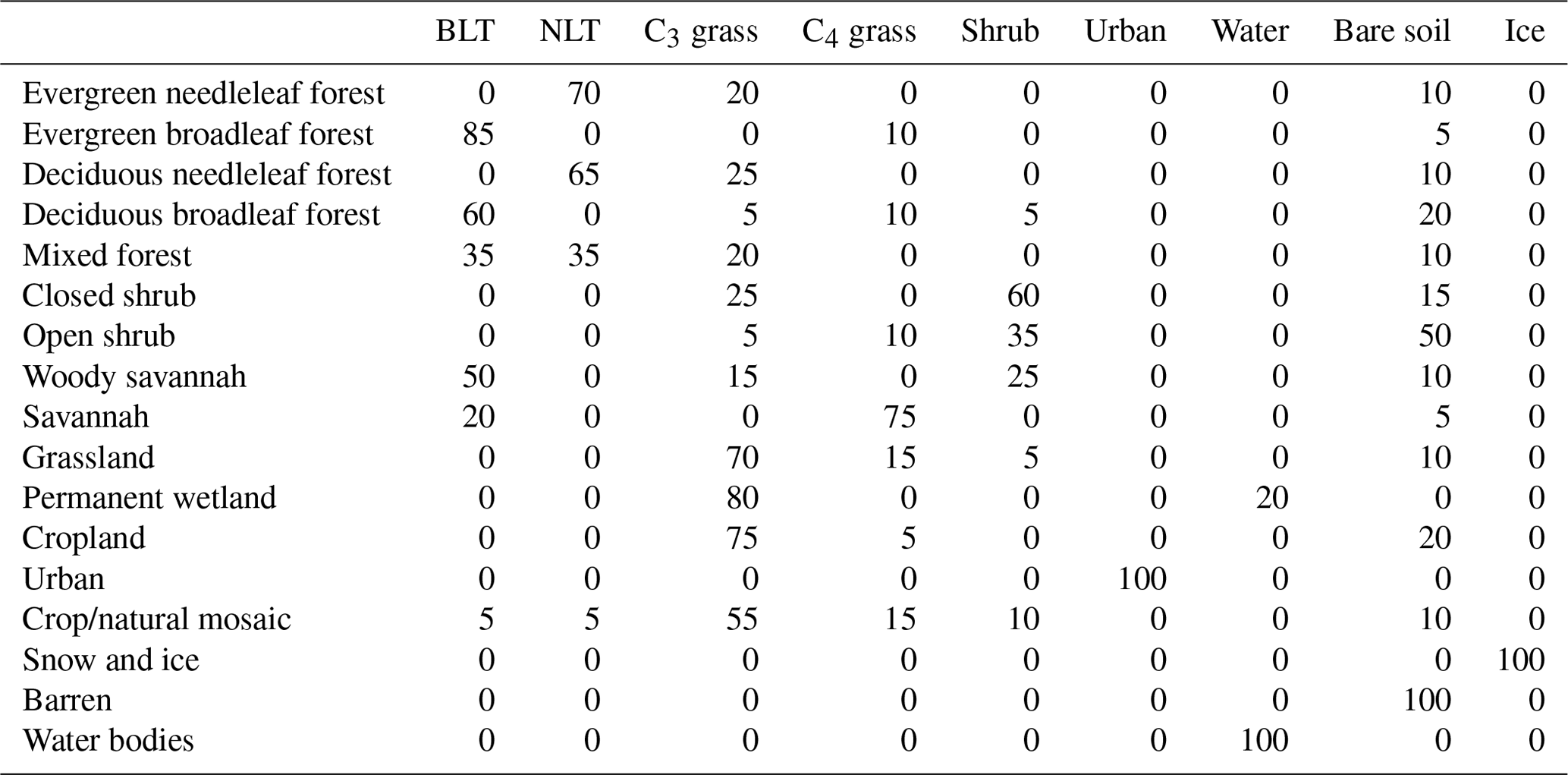
Table B2 Leaf area index lookup table for combinations of IGBP land cover class and plant functional type. These lookup tables are used in conjunction with Eqs. (1) and (2).

Table B3 PFT-dependent canopy height scaling factor.