Implementation and application of ensemble optimal interpolation on an operational chemistry weather model for improving PM_2.5 and visibility predictions

Data assimilation techniques are one of the most important ways to reduce the uncertainty in atmospheric chemistry model input and improve the model forecast accuracy. In this paper, an ensemble optimal interpolation assimilation (EnOI) system for a regional online chemical weather numerical forecasting system (GRAPES_Meso5.1/CUACE) is developed for operational use and efficient updating of the initial fields of chemical components. A heavy haze episode in eastern China was selected, and the key factors affecting EnOI, such as localization length scale, ensemble size, and assimilation moment, were calibrated by sensitivity experiments. The impacts of assimilating ground-based PM_2.5 observations on the model chemical initial field PM_2.5 and visibility forecasts were investigated. The results show that assimilation of PM_2.5 reduces the uncertainty in the initial PM_2.5 field considerably. Using only 50 % of observations in the assimilation, the root mean square error (RMSE) of initial PM_2.5 for independent verification sites in mainland China decreases from 73.7 to 46.4 µg m⁻³, and the correlation coefficient increases from 0.58 to 0.84. An even larger improvement appears in northern China. For the forecast fields, assimilation of PM_2.5 improves PM_2.5 and visibility forecasts throughout the time window of 24 h. The PM_2.5 RMSE can be reduced by 10 %–21 % within 24 h, and the assimilation effect is the most remarkable in the first 12 h. Within the same assimilation time, the assimilation efficiency varies with the discrepancy between model forecasts and observations at the moment of assimilation, and the larger the deviation, the higher the efficiency. The assimilation of PM_2.5 further contributes to the improvement of the visibility forecast. When the PM_2.5 increment is negative, it corresponds to an increase in visibility, and when the PM_2.5 analysis increment is positive, visibility decreases. It is worth noting that the improvement of visibility forecasting by assimilating PM_2.5 is more obvious in the light-pollution period than in the heavy-pollution period. The results of this study show that EnOI may provide a practical and cost-effective alternative to the ensemble Kalman filter (EnKF) for the applications where computational cost is the main limiting factor, especially for real-time operational forecast.

1 Introduction

Air pollution is an intractable problem that most developing countries in the world with high populations are facing at present. PM_2.5 plays an important role in air pollution, and its concentration will directly affect air quality. From a health perspective, long-term exposure to high concentrations of PM_2.5 has adverse effects on the human body and respiratory system and can lead to cardiovascular disease and other chronic diseases (Ghorani-Azam et al., 2016). From a meteorological perspective, aerosol particles can absorb and scatter solar radiation effectively, change the intensity and direction of sunlight, and reduce atmospheric horizontal visibility (Liu et al., 2019; Yadav et al., 2022; Ting et al., 2022), leading to haze episodes, which are characterized by significant growth in the concentration of aerosol particles and sharp reduction in visibility.

Accurate PM_2.5 and visibility forecasts are critical for human health, air quality assessment, and public transportation safety issues (Hu et al., 2013). Chemistry transport models (CTMs) or coupled chemistry–meteorology models (CCMMs) are important tools for PM_2.5 and visibility forecasting and are pivotal in air quality and atmospheric chemistry research. However, various uncertainties exist in the simulation of atmospheric components by CTMs or CCMMs, especially for aerosols (Lee et al., 2016). The complexity of atmospheric pollution formation mechanisms and model structure, the uncertainty in chemical initial conditions (ICs), and the lag in emission inventories lead to a deviation of air quality forecast results from observed comparisons.

Data assimilation (DA) is one of the most effective ways to improve model predictions. Weather prediction has been relying on data assimilation for many decades (Kalnay, 2003; Navon, 2009). In comparison, the use of data assimilation in atmospheric chemistry models to improve air quality forecasting is more recent, but important advances have been made. Tombette et al. (2009) presented an experiment on PM₁₀ data assimilation using the optimal interpolation (OI) method to improve PM₁₀ forecasting. Tang et al. (2015) used the same DA method to assimilate ozone, PM_2.5, and MODIS aerosol optical depth (AOD) data into the Community Multiscale Air Quality (CMAQ) model to improve the ozone and total aerosol concentration for the CMAQ simulation over the contiguous United States. Liu et al. (2011) assimilated AOD from the Terra and Aqua satellites using the GSI 3D-Var assimilation system, showing that AOD data assimilation systems can serve as a tool to improve simulations of dust storms. Li et al. (2013) and Feng et al. (2018) assimilated ground-based observations of PM_2.5 using 3D-Var to improve PM_2.5 forecasting. 4D-Var has successfully been implemented on CTMs and has improved the PM_2.5 forecasting capability. Zhang et al. (2016) constructed a GEOS-Chem adjoint model suitable for PM_2.5 pollution diffusion based on a 4D-Var algorithm, which was verified by the monitoring data of the Asia-Pacific Economic Cooperation Summit in Beijing in 2014. Zhang et al. (2021) built a PM_2.5 data assimilation system based on the 4D-Var algorithm and the WRF-CMAQ model, which can assimilate synchronous observations simultaneously to improve aerosol prediction accuracy. Wang et al. (2021) established a 4D-Var assimilation system based on GRAPES_CUACE to optimize black carbon (BC) daily emissions in northern China on 4 July 2016. The ensemble Kalman filter (EnKF) also plays a significant role in improving the accuracy of atmospheric chemistry model forecasts. Lin et al. (2008) developed an EnKF system for a regional dust transport model. Tang et al. (2011) investigated a cross-variable ozone DA method based on an EnKF for improving ozone forecasts over Beijing and surrounding areas. Park et al. (2022) developed a DA system for the CTM using the EnKF technique, where PM_2.5 observations from ground stations are assimilated to ICs every 6 h to improve PM_2.5 forecasting in the Korean region. Peng et al. (2017) used EnKF to optimize ICs and emission input, resulting in significant improvements in PM_2.5 forecast. Overviews of these achievements have been provided in the literature (Bocquet et al., 2015; Benedetti et al., 2018; Zhu et al., 2018; Sokhi et al., 2022).

Although previous studies have reported DA methods using ground-based or satellite-retrieved observation led to the improvement of atmospheric composition prediction, each of these DA methods has its own limitation. In OI and 3D-Var, the background error covariance (BEC) matrix is estimated at once, and the prediction error is statistically stationary. 4D-Var and EnKF are advanced data assimilation methods that provide the evolution of the forecast error covariance, but when they are employed in the operation use, each of them faces their own challenge. The CTM and CCMM are complex systems with rapid updates, and the implementation of 4D-Var requires a large workload of adjoint model coding (Ha, 2022). EnKF obtains a flow-dependent BEC using ensemble forecast by integrating the model multiple times, and that makes it approximately 100 times more computationally expensive than the forward model when applied to nonlinear systems (Counillon and Bertino, 2009). Compared to EnKF, EnOI is a suboptimal method for ensemble-based assimilation (Evensen, 2003). EnOI uses a stationary ensemble to estimate the BEC, and only one analysis field is updated at a time, which makes the computation time greatly reduced. EnOI can be used in conjunction with other DA methods and may be an appropriate choice for coupled forecast systems (Oke et al., 2010). EnOI has widely been used in ocean models with significant improvements to model forecast (Xie and Zhu, 2010; Castruccio et al., 2020; Belyaev et al., 2021) but not in the CTM or CCMM. To our knowledge, there have only been a few papers involved in research of EnOI in atmospheric chemistry models so far. Zhang et al. (2014) implement EnOI on an air quality numerical modelling for the Pearl River Delta region in China. They found that EnOI produced the initial condition closer to the true situation, but they did not investigate the effect of EnOI on forecast. Wang et al. (2016) used EnOI to investigate the possibility of optimally recovering the spatially resolved emissions bias of black carbon aerosol. Wu et al. (2021) applied EnOI to assimilate hourly surface observations of CO concentrations at 1107 sites over China in January 2015. They found that simulations with the updated emissions revealed a decreased bias of average CO concentrations at 349 independent validation sites from 0.74 to 0.01 mg m⁻³ and a reduction in the RMSE by 18 %. Results from these papers showed that EnOI is a useful and computation-free method to reduce the errors of the initial chemical condition or emissions. Since the development of CCMMs is fairly recent, EnOI has not applied for real-time CCMM yet. The GRAPES-CUACE is an online CCMM system developed by the China Meteorological Administration (Gong and Zhang, 2008; Zhou et al., 2008; Wang et al., 2010a). This model plays an important role not only in the scientific research on air pollution (Wang et al., 2015a, b), aerosol–cloud interaction (Wang et al., 2018; Peng et al., 2021), and aerosols' weather feedback (Wang et al., 2010b; Zhang et al., 2022), but also in the operational forecasting of air quality, fog–haze weather, and dust storms in China (Wang and Niu, 2013; Liu et al., 2017). Very recently has this model system been updated to a new version (GRAPES_Meso5.1/CUACE) with many improvements (Wang et al., 2022). In this study, we established a real-time EnOI chemistry initial field PM_2.5 assimilation system for this new version of the model, by assimilating PM_2.5 data from nearly 1500 ground stations in China into the model chemical initial fields to improve the model forecasts of the concentrations of PM_2.5 and discuss the impact of assimilating PM_2.5 on visibility.

2 Methods and data

2.1 The ensemble optimal interpolation algorithm

The EnOI algorithm used in this study is based on the work of Evensen (2003). A brief recall of the EnKF and EnOI is given in this section. DA methods are algorithms that combine observations and model results and their respective statistical characteristics of errors to obtain a statistically optimal analysis value by minimizing the analysis variance. Based on Kalman filter theory, the analysis stateψ^a is determined by a linear combination of the vector of measurements y and the forecasted model state vector or background ψ^f, which is given by Eqs. (1) and (2),

$$\begin{array}{}\text{(1)}& {\displaystyle }{\mathit{\psi }}^{\mathrm{a}}={\mathit{\psi }}^{\mathrm{f}}+\mathbf{K}\left(\mathit{y}-\mathbf{H}{\mathit{\psi }}^{\mathrm{f}}\right),\text{(2)}& {\displaystyle }\mathbf{K}={\mathbf{PH}}^T{\left[{\mathbf{HPH}}^T+\mathbf{R}\right]}^{-\mathrm{1}},\end{array}$$

where K is the Kalman gain matrix, P is the background error covariance matrix, H is the observation operator that relates the model state to the observation, and R is the observation error covariance matrix.

Now we define A as the matrix holding the ensemble members ψ_i,

$$\begin{array}{}\text{(3)}& \mathbf{A}=\left({\mathit{\psi }}_{\mathrm{1}},{\mathit{\psi }}_{\mathrm{2}},\mathrm{\cdots },{\mathit{\psi }}_N\right)\in {\mathbf{R}}^{{\mathit{n}}_{\dim }\times N},\end{array}$$

where N is the number of ensemble members, and n_dim is the size of the model state vector. Let $\stackrel{\mathrm{‾}}{A}$ be the ensemble mean of A; then the ensemble anomaly A^′ is defined as

$$\begin{array}{}\text{(4)}& \mathbf{A}{}^{\prime }=\mathbf{A}-\stackrel{\mathrm{‾}}{\mathbf{A}}.\end{array}$$

The ensemble covariance matrix P can be defined as

$$\begin{array}{}\text{(5)}& \mathbf{P}={\displaystyle \frac{\mathbf{A}{}^{\prime }{{\mathbf{A}}^{\prime }}^T}{N-\mathrm{1}}}\in {\mathbf{R}}^{n_{\dim }\times n_{\dim }}.\end{array}$$

The vector of measurements y needs to be perturbed with its error as the following:

$$\begin{array}{}\text{(6)}& {\mathit{d}}_j=\mathit{y}+{\mathit{\epsilon }}_j,j=\mathrm{1},\mathrm{\cdots },N,\end{array}$$

which can be stored in a matrix as

$$\begin{array}{}\text{(7)}& \mathbf{D}=\left({\mathit{d}}_{\mathrm{1}},{\mathbf{d}}_{\mathrm{2}},\mathrm{\cdots },{\mathit{d}}_n\right)\in {\mathbf{R}}^{m\times N},\end{array}$$

where m is the number of measurements.

The EnKF analysis equation will be expressed as the following:

$$\begin{array}{}\text{(8)}& \begin{array}{rl}{\mathbf{A}}^a& =\mathbf{A}+{\mathbf{A}}^{\prime }{{\mathbf{A}}^{\prime }}^T{\mathbf{H}}^T{\left[{\mathbf{HA}}^{\prime }{{\mathbf{A}}^{\prime }}^T{\mathbf{H}}^T+\left(N-\mathrm{1}\right)\mathbf{R}\right]}^{-\mathrm{1}}\\ & \left(\mathbf{D}-\mathbf{HA}\right).\end{array}\end{array}$$

The analysis includes updating each ensemble and needs to run the model N times in every forecast cycle to calculate P; therefore it tends to be computationally demanding and has limited use when the computer time is the main affecter to be considered, especially in real-time operational forecast.

The EnOI analysis is computed with the ensemble covariance matrix P spanned by a stationary ensemble of model states sampled from a long time integration. It is computed by solving an equation written as the following:

$$\begin{array}{}\text{(9)}& \begin{array}{rl}{\mathit{\psi }}^{\mathrm{a}}& ={\mathit{\psi }}^{\mathrm{f}}+\mathit{\alpha }{\mathbf{A}}^{\prime }{{\mathbf{A}}^{\prime }}^T{\mathbf{H}}^T{\left[\mathit{\alpha }{\mathbf{HA}}^{\prime }{{\mathbf{A}}^{\prime }}^T{\mathbf{H}}^T+\left(N-\mathrm{1}\right)\mathbf{R}\right]}^{-\mathrm{1}}\\ & \left(\mathit{y}-\mathbf{H}{\mathit{\psi }}^{\mathrm{f}}\right),\end{array}\end{array}$$

where the scalar $\mathit{\alpha }\in \left(\mathrm{0},\left.\mathrm{1}\right]\right.$ is introduced to allow for different weights on the ensemble versus measurements. As Evensen (2003) pointed out, an ensemble consisting of model states sampled over a long time period will have a climatological variance which is too large to represent the actual error in the model forecast, and α, which mainly depends on how the model forecast behaviour is used to reduce the variance to a realistic level and can be tuned for optimal performance. In this study, it is taken as 0.9 based on our experience. Through Eq. (9) the EnOI analysis updates only one model state at a time, so the computer time can be reduced by 1 or 2 orders of magnitude.

2.2 The EnOI data assimilation system design

Using a set of ensemble forecasts with a finite number to calculate the BEC will suffer from sample error and cause imperfect estimation or even filter divergence (Houtekamer and Mitchell, 1998). There are two sorts of techniques to possibly solve this problem. One is the distance-dependent covariance localization, which is done by updating the analysis at all grid points with the multiplication of the BEC by a correlation function (Hamill et al., 2001). The other is done by updating the analysis at each grid point simultaneously using the state variables and the observations in the local region centred at that point (Ott et al., 2004). In our EnOI DA system, we use the second technique. First, we define the localization length scale as L. For each model grid point, we find the observations within L which are called active observations, and then calculate the corresponding innovation. This localization effect on the analysis is illustrated in Sect. 1 (Fig. 3).

The observation error covariance matrix R is assumed to be diagonal here; that is, the observation errors are not correlated. The diagonal elements of R are thus given by the sum of the measurement error variance ${\mathit{\epsilon }}_{\mathrm{o}}^{\mathrm{2}}$ and representativeness error variance ${\mathit{\epsilon }}_{\mathrm{r}}^{\mathrm{2}}$, following Elbern et al. (2007). The measurement error ε_o is assigned as 7.5 % of the observed value, and the representativeness error ε_r is formulated as ${\mathit{\epsilon }}_{\mathrm{r}}={\mathit{\epsilon }}_{\mathrm{o}}\cdot \sqrt{\frac{\mathrm{\Delta }x}{L_{\mathrm{r}}}}$, where Δx is the model grid resolution (10 km in this study), and L_r is the characteristic representativeness length of the observation, defined as 2 km for urban sites, 10 km for rural sites, and 20 km for remote sites.

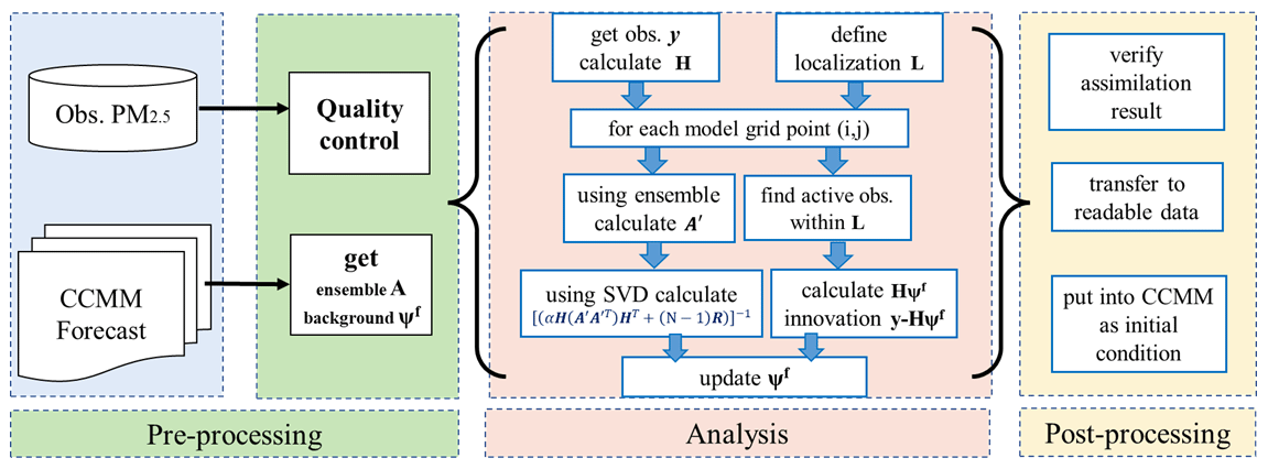
Figure 1 Flowchart of the main procedures for the EnOI initial field assimilation system. The obs. PM_2.5 is the ground-based observation of PM_2.5. The CCMM is a coupled chemistry–meteorology model. SVD is the singular value decomposition.

Based on Eq. (9), we built the EnOI initial field PM_2.5 assimilation system, as shown in Fig. 1. The main procedures can be divided into pre-processing, analysis, and post-processing. Pre-processing involves the acquisition of observed data and ensemble samples. Analysis is the revised main module of EnOI where the main computational processes are performed. Post-processing firstly verifies the assimilation results using the validation observations which are not used in EnOI and then processes the results obtained from assimilation into model-readable chemical initial conditions. Compared with the traditional EnOI, the time-continuous model historical forecast before the assimilation moment is selected as the ensemble samples for this study. The ensemble design is set to be as follows: suppose the assimilation will be done at time t, first we evolve the model from the spin-up run at t−NΔt and integrate the model into time t (in our operational set-up, Δt is 1 h); therefore we get a time series of N-hourly model forecast outputs, ${\mathit{A}}_{t-N+\mathrm{1}}$, ${\mathit{A}}_{t-N+\mathrm{2}}$, …, A_t−1, A_t. These hourly outputs before the assimilation time t form the N-number ensemble A, which can be used to calculate the average $\stackrel{\mathrm{‾}}{\mathbf{A}}$ and anomalous A^′, and then the background error covariance matrices P is calculated. The BEC is stationary for a particular analysis moment, but it changes with the assimilation moment during a long assimilation period. Because background error covariance statistics are derived directly from forecasts, and the DA scheme does not need to modify the original CCMM, EnOI is very easy to apply and cost-free in terms of computation time.

2.3 GRAPES_Meso5.1/CUACE

In this study, the DA method EnOI was established for the latest updated version of the regional atmospheric chemistry model GRAPES_Meso5.1/CUACE developed by the China Meteorological Administration (Wang et al., 2022). The model system is established by online coupling the Chinese Unified Atmospheric Chemistry Environment (CUACE) model with the meteorology model GRAPES_Meso5.1. GRAPES_Meso refers to a real-time operational weather forecasting model used by the China Meteorological Administration (Chen et al., 2008; Zhang and Shen, 2008). Now, the new version of it has been established with resolutions ranging from 3 to 10 km for regional forecast (Shen et al., 2020). It uses fully compressible non-hydrostatic equations as its model core. The vertical coordinates adopt the height-based, terrain-following coordinates, and the horizontal coordinates use the spherical coordinates of equal latitude–longitude grid points. The horizontal discretization adopts an Arakawa-C staggered grid arrangement and a central finite-difference scheme with second-order accuracy, while the vertical discretization adopts the vertically staggered variable arrangement. The time integration discretization uses a semi-implicit and semi-Lagrangian temporal advection scheme. The transport and advection processes for all gases and aerosols are calculated by the dynamic framework of GRAPES_Meso5.1. The second component, CUACE, refers to the atmospheric chemistry model, which mainly includes three modules: the aerosol module, the gaseous chemistry module, and the thermodynamic equilibrium module. In the gaseous chemistry module, 63 gas species through 21 photochemical reactions and 136 gas-phase reactions participate in the calculations. The aerosol module considers the dynamic, physical, and chemical processes of aerosols, including hygroscopic growth, dry and wet depositions, condensation, nucleation, vertical mixing, cloud chemistry, and coagulation and activation of cloud condensation nodules from aerosols. Seven types of aerosols (sea salt, sand/dust, black carbon, organic carbon, sulfate, nitrate, and ammonium salt) are considered. The aerosol size spectrum (except for ammonium salt) is divided into 12 bins with a particle radium of 0.005–0.01, 0.01–0.02, 0.02–0.04, 0.04–0.08, 0.08–0.16, 0.16–0.32, 0.32–0.64, 0.64–1.28, 1.28–2.56, 2.56–5.12, 5.12–10.24, and 10.24–20.48 µm. The interface programme that connects CUACE and GRAPES_Meso transmits the meteorological fields calculated in GRAPES_Meso and the emission data processed as needed to each module of CUACE.

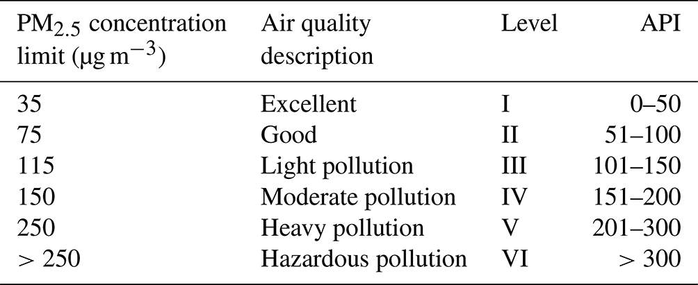
Table 1 Mass concentration limit of PM_2.5 and its corresponding air quality level and air pollution index (API).

Table 2 Experimental design.

2.4 Data

Based on the Ambient Air Quality Standards (GB 3095-2012) of China, the mass concentration limit of PM_2.5 and its corresponding air quality level and air pollution index (API) are shown in Table 1. Haze is defined as a weather phenomenon caused by air pollution when visibility is less than 10 km according to the Observation and Forecasting Levels of Haze (QX/T 113-2010) of China. Three pollution episodes occurred in China in December 2016, with the most severe haze episode occurring in China from 16 to 21 December 2016 (see more details in Wang et al., 2022, Table 3). During this pollution episode, the highest daily PM_2.5 concentration peaked to 600 µg m⁻³ in Shijiazhuang and some other cities, reaching the severely polluted level (250–500 µg m⁻³). In this study, 15–23 December 2016 was selected as the main study period, and both model input data and observation data used in this study are within this month. Model input data include anthropogenic emission data, model meteorological initial data, and boundary data. The emission inventory used in this study is from the Multi-resolution Emission Inventory for China (MEIC) in December 2016 (http://www.meicmodel.org/, last access: 16 May 2022). The emission inventory covers power plants, industry (cement, iron and steel, industrial boilers, the petroleum industry), the residential sector, transportation, solvent use and agriculture, and in-field crop residue burning. The National Centers for Environmental Prediction (NCEP) final analysis (FNL) data (https://rda.ucar.edu/datasets/ds083.3/, last access: 3 April 2022) are used for the model's initial and 6 h meteorological lateral boundary input fields. The observations include PM_2.5 and visibility. Nearly 1500 ground-based hourly PM_2.5 (µg m⁻³) observations from the Chinese Ministry of Environmental Protection with detailed locations and spatial distributions of the stations are shown in Fig. 2. The hourly meteorological automatic ground-based visibility data (km) were obtained from the China Meteorological Administration. The time format of these observations is processed to UTC, and all the observational data are obtained after quality control and rechecked before use.

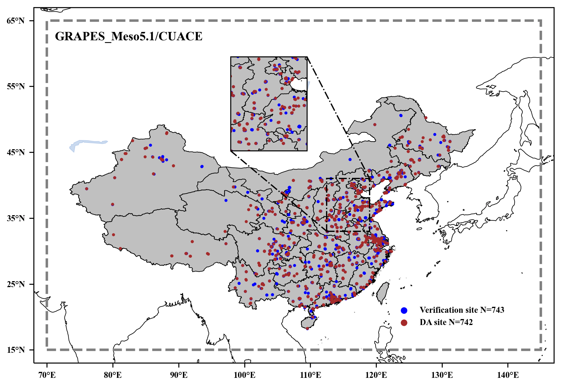
Figure 2 Simulation domain of GRAPES_Meso5.1/CUACE. The minor region represents northern China (NC). The locations of the ground stations in mainland China are marked on the maps with blue and brown dots. The blue and brown dots represent verification sites and assimilation sites, respectively. N=743 means there are 743 verification sites. N=742 means there are 742 DA sites.

2.5 Experimental set-up

The horizontal resolution, time step, forecast length, and model domain of the GRAPES_Meso5.1/CUACE model are optional. In this study, the horizontal resolution of the model is $\mathrm{0.1}{}^{\circ }\times \mathrm{0.1}{}^{\circ }$; the time step is 100 s considering the model's integration stability and accuracy; and the model domain is 70–145^∘ N, 15–60^∘ E (dashed grey box in Fig. 2). There are 49 model layers ascending vertically from the surface to 31 km in height. The model warm restart time is 00:00 and 12:00 UTC, and the forecast length is 24 h. The model simulation results are output on an hourly basis.

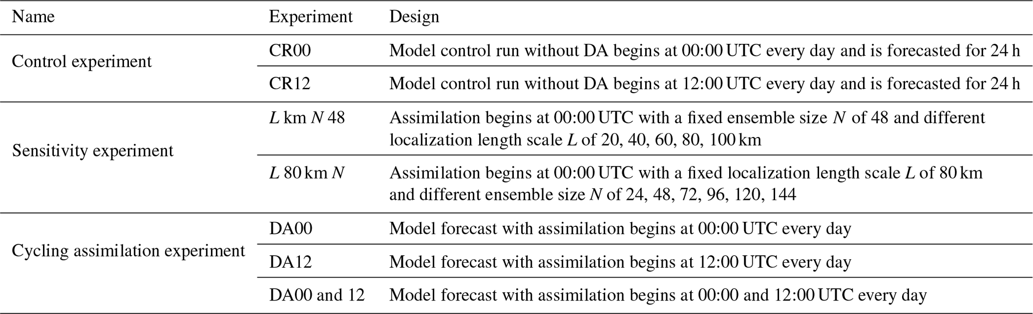
Three groups of experiments were performed in this study: one set of control experiments (CRs), one set of sensitivity experiments, and one set of cyclic DA experiments, as shown in Table 1. CR00 is the control experiment representing a model run without DA beginning at 00:00 UTC every day and forecasted for 24 h (the initial field is the previous day's 24 h forecast field), simulated from 1 to 31 December 2016. CR12 is also a model run without DA but begins at 12:00 UTC every day and is forecasted for 24 h. The localization length scale L and the ensemble size N are the key parameters affecting EnOI. Based on CR00, two parallel sensitivity experiments were designed to study the impact of the localization length scale and ensemble size on the assimilation effects. The chemical initial field ensemble samples for the sensitivity experiments were obtained from the CR00. The first group of sensitivity experiments is fixed with ensemble size N of 48, and the length scale is selected for 20, 40, 60, 80, and 100 km to investigate the impacts of different localization length-scale choices on the optimized chemical initial field; the second group is fixed with length scale L of 80 km, and the 24, 48, 72, 96, 120, and 144 simulations before the assimilation moment (00:00 UTC) were selected as ensemble samples, respectively, and the effect of the number of ensemble samples on the assimilation effect was discussed.

To investigate the impact of the assimilation moment on the forecast fields, the optimal length scale and ensemble size were selected based on the results of sensitivity experiments, and two sets of cyclic DA experiments, DA00 and DA12, were set up to represent the daily assimilation of the initial fields at 00:00 and 12:00 UTC, respectively. The N-hourly model forecasts before the assimilation moment were used as the ensemble samples to approximate the BEC, and the analysis increments were calculated by combining the model forecasts and PM_2.5 observations at 00:00 and 12:00 UTC, and the analysis was used as the chemical initial fields for the next forecast to achieve cyclic DA.

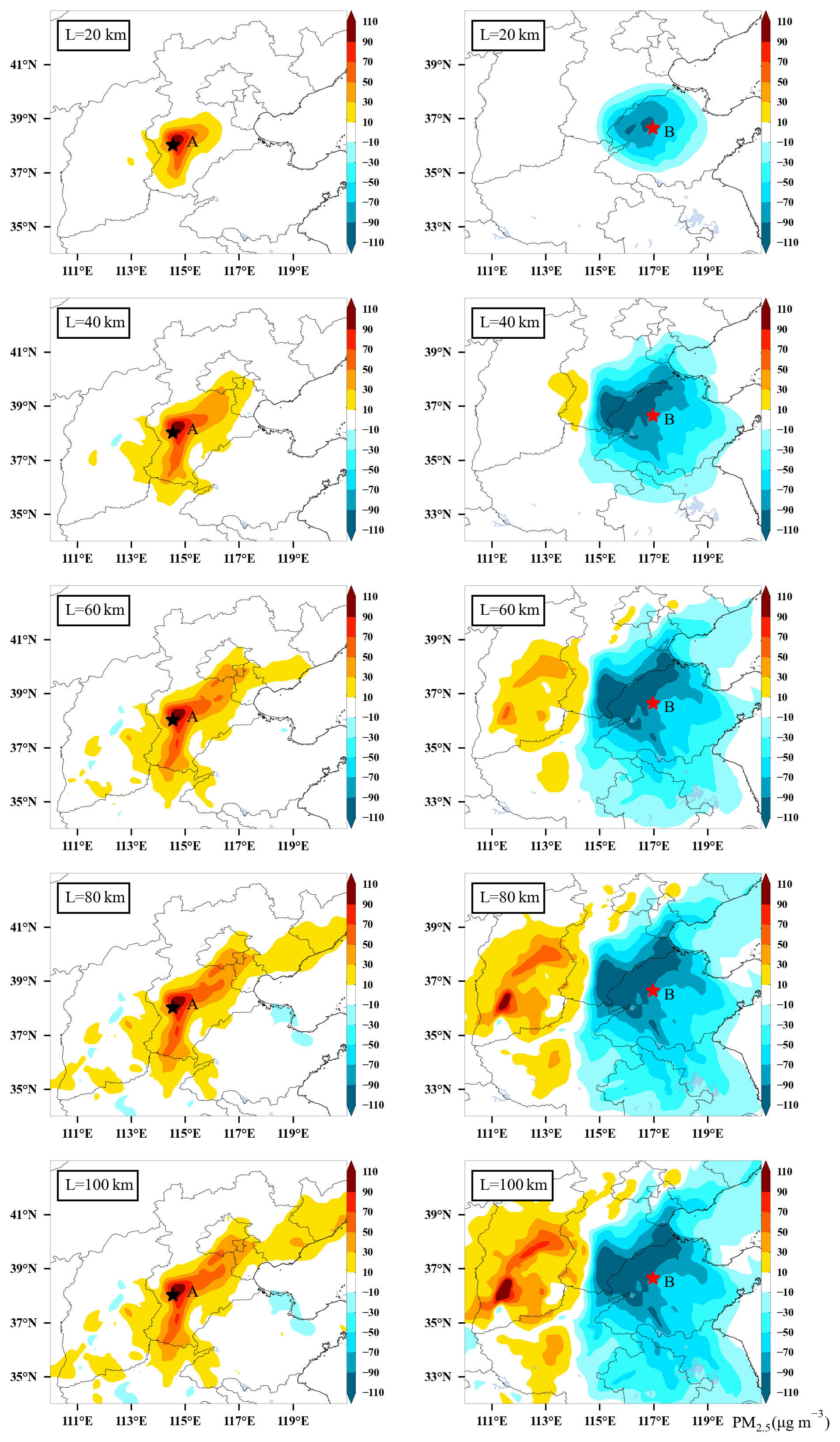
Figure 3 Spatial distribution of PM_2.5 analysis increments after assimilation of initial fields at 00:00 UTC on 15 December 2016 for assimilation site A (38.0^∘ N, 114.5^∘ E) only (left column) and assimilation site B (36.6^∘ N, 116.9^∘ E) only (right column) with a fixed ensemble size of 48 and different localization length scales of 20, 40, 60, 80, and 100 km.

3 Results and discussion

3.1 Sensitivity experiments of localization length scale

The localization effect on the analysis is illustrated first, and two observation sites, A (38.0^∘ N, 114.5^∘ E) and B (36.6^∘ N, 116.9^∘ E), were selected to perform a length-scale single-point experiment for the initial field at 00:00 UTC on 15 December 2016, corresponding to the left and right columns of the analysis increments (ψ^a−ψ^f) shown in Fig. 3. The analysis increments are determined by both the observation increments and the BEC based on Eq. (9). As shown in Fig. 3, the increments are positive in the left and negative in the right column, which represents the underestimation of PM_2.5 concentration at site A and overestimation at site B before being assimilated. As the length scale increases, the range of the analysis increment expands, and the number of model grids that can be affected increases gradually. Due to the sparse distribution of PM_2.5 sites, if the localization length scale is too small, most of the model grids cannot be updated, which reduces the assimilation efficiency, whereas if the localization length scale is too large, the analysis increments between distant sites will offset and superimpose, creating fake increments. With the experiments using length scales of L=80 and 100 km, small negative analysis increments are found at site A in the southeastern direction. Compared to site A, wide positive analysis increments that do not match the actual situation are found at site B in the western direction for experiments using L=60, 80, and 100 km. It is worth noting that there are differences in the shape of the analysis increment fields at sites A and B, which are related to EnOI having a flow-dependent BEC. The details of BEC will be discussed in Sect. 3.2.

Table 3 Statistics of PM_2.5 concentrations for verification sites of the initial field without (CR) and with assimilation at 00:00 UTC each day from 1 to 31 December 2016. Assimilation sensitivity experiments were performed with 48 ensemble samples and length scale L of 20, 40, 60, 80, and 100 km, respectively, and only assimilated the assimilation sites.

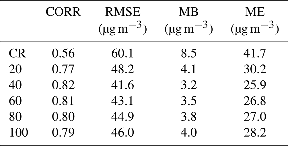
Ground-based PM_2.5 sites are established according to the population and economic development level of the region and are not evenly distributed, such as Beijing, Shanghai, Guangzhou, and other economically developed and populous megacities, which have a high density of PM_2.5 sites, while the western and central regions of China are sparsely populated, and the sites are partially sparse. So, in order to obtain the statistically optimal localization length scale, we performed assimilation experiments on the initial fields at 00:00 UTC each day from 1 to 31 December. A total of 50 % of PM_2.5 sites were randomly selected as DA sites, and the rest were used as verification sites (without DA). The blue and brown sites shown in Fig. 2 represent the spatial distribution of verification and assimilation sites, respectively. The statistics results of verification sites against the observation are shown in Table 3. Compared to the CR, the correlation coefficient (CORR) of DA for verification sites increases from 0.65 to 0.77 at least, and the root mean square error (RMSE), mean bias (MB), and mean error (ME) of the DA experiment are smaller than those of the CR. The statistical data are different for different localization length scales, indicating that localization can have an effect on the assimilation. Compared with the CR, the RMSE of DA decreased from 60.1 to 41.6 µg m⁻³, MB decreased from 8.5 to 3.2 µg m⁻³, and ME decreased from 41.73 to 25.9 µg m⁻³ for the localization length-scale selection of 40 km, which is the best among all the experiments on different length scales. Localization length scales of 60 and 80 km have similar statistics results, but the statistics of 20 and 100 km are not very good. Using a localization length scale of 20 km prevents most of the model data from being updated, while using too large a length scale allows remote sites to interact with each other and produce more spurious increments. In addition, from the meteorological conditions, heavy-pollution weather is always characterized by small or static winds and pollutant transport over small distances. An observation site represents a limited spatial extent, so a larger localized length-scale setting may also not produce a very realistic initial field. From this sensitivity experiment, we find that when the localization length scale used is from 40 km to 80 km, the statistics are relatively good, and the optimal assimilation effect can be achieved.

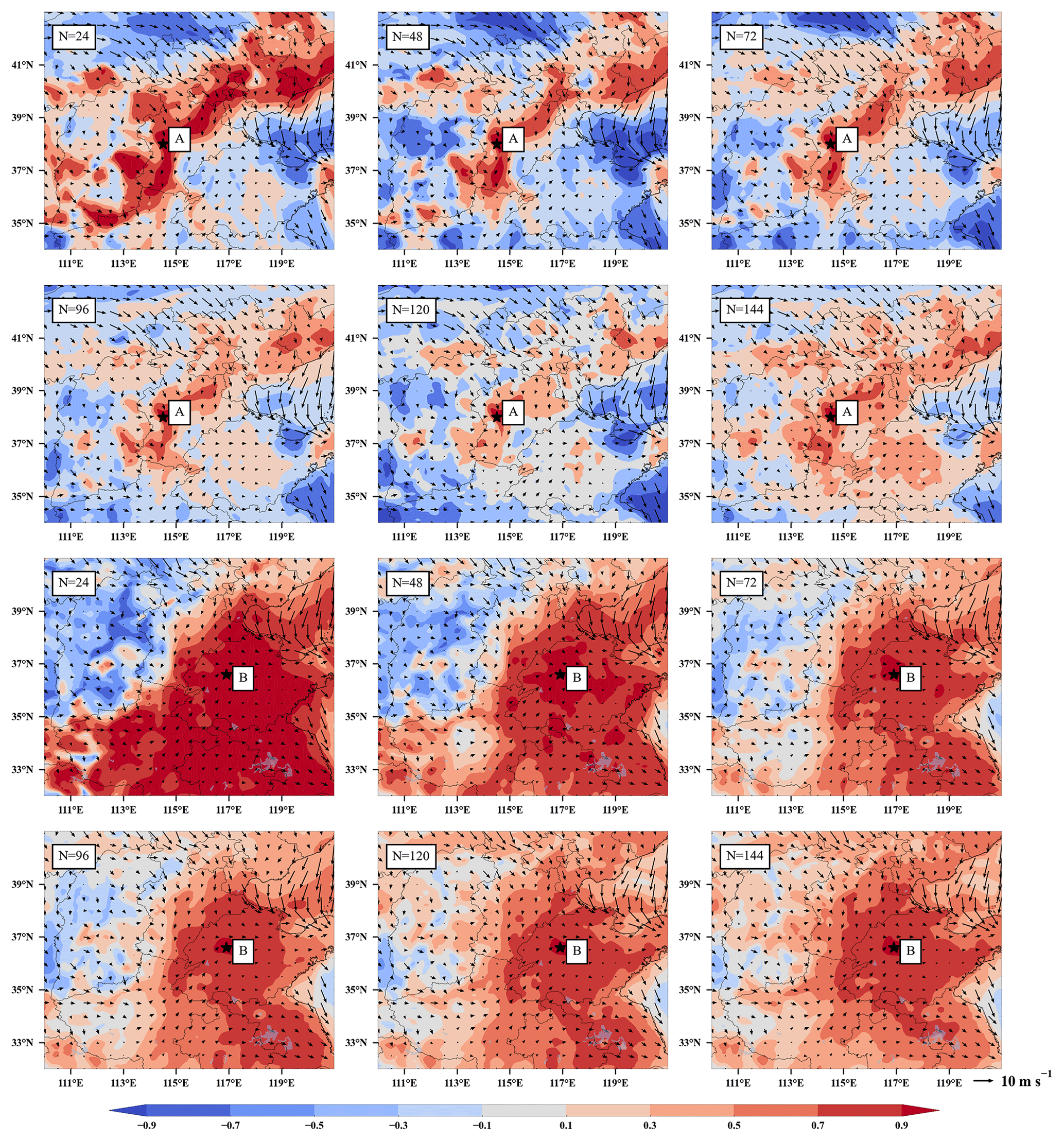
Figure 4 Spatial distribution of correlation coefficients of background error for site A (38.0^∘ N, 114.5^∘ E) (rows 1, 2) and site B (36.6^∘ N, 116.9^∘ E) (rows 3, 4) with different ensemble size N of 24, 48, 72, 96, 120, and 144 and wind vectors at 00:00 UTC on 15 December 2016.

3.2 Sensitivity experiments of ensemble size

We repeat the series of experiments presented in Fig. 3 but with a localizing length scale of 80 km and 24, 48, 72, 96, and 120 ensemble members. Figure 4 shows a map of the BEC correlation field between observation sites (A, B) for different ensemble sizes, overlaid with the 00:00 UTC surface wind vector of 15 December 2016. Site A is controlled by strong northern and northwestern winds, which makes the CORR field show a northeast–southwest trend. The wind speed at site B is less than 5 m s⁻¹ in all directions with a steady state, so the CORR field is approximately distributed in concentric circles nearby the centre of the site. As the number of ensemble samples increases, the area of positive CORR greater than 0.7 gradually increases in A and B. The ensembles of size N=24 or N=48 can be considered small compared to the selection of other ensemble sizes in sensitivity experiments. In this case, the CORRs between the observation sites and the surrounding large-scale areas are all greater than 0.7, and an extremely strong negative correlation is found in the southwest. The success of ensemble-based DA systems depends strongly on the number of samples. The smaller ensemble size fails to accurately estimate the BEC and is prone to sampling error, resulting in an overestimation or underestimation of the initial field, and Natvik and Evensen (2003) investigated the effect of the number of samples on assimilation and showed that an ensemble of fewer than 60 samples reduces the performance of assimilation. When the hourly model forecasts of over 5 d (N=120) before assimilation are selected as the ensemble samples, the correlations of both sites A and B with the BECs in a wide area become positive.

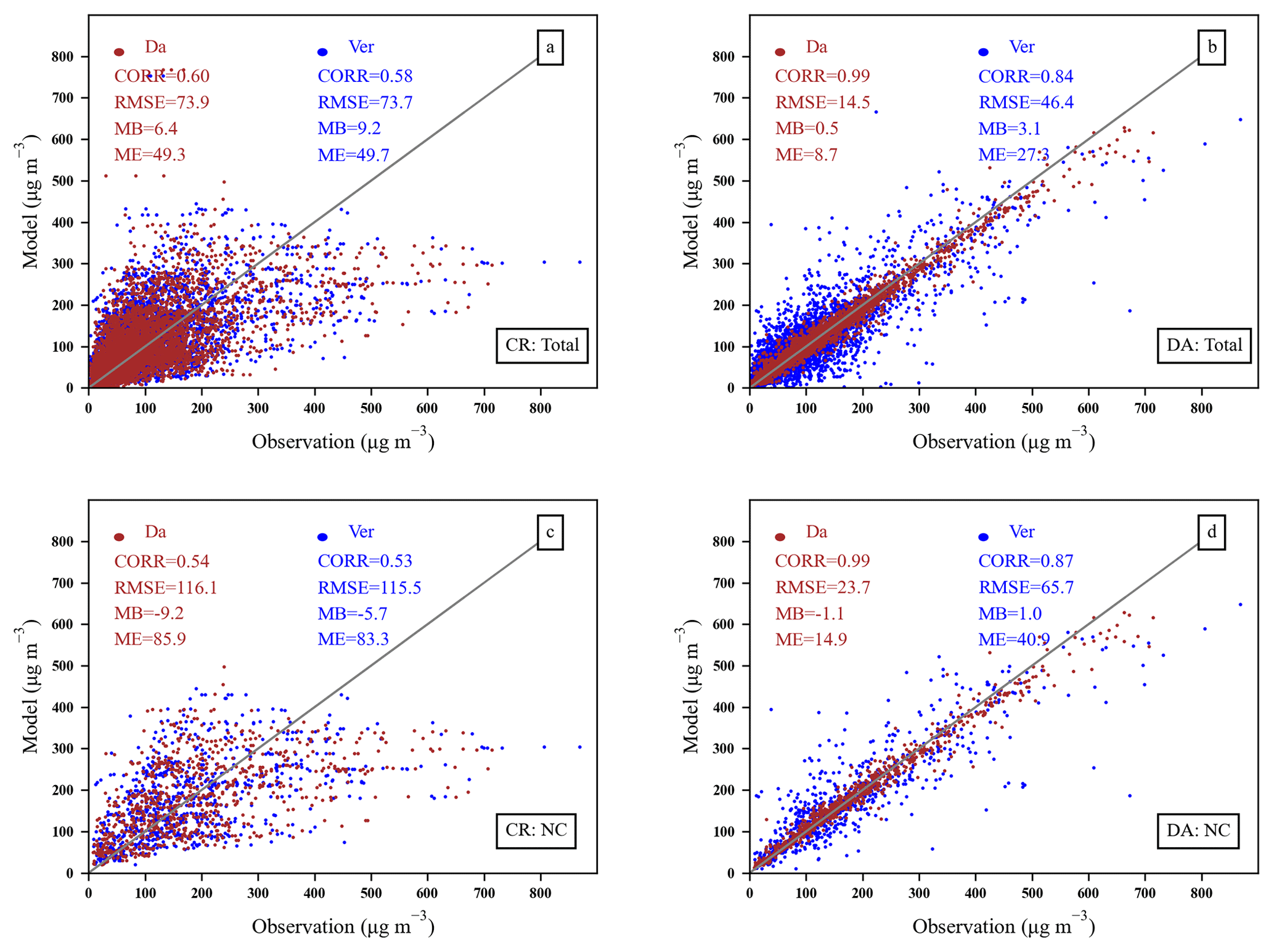
Figure 5 Scatterplot of PM_2.5 concentrations from the control experiment (a, c) and the assimilation experiment (b, d). The ensemble size in the assimilation experiment is 96, and the length scale L is 40 km. Brown (Da) and blue (Ver) dots are assimilation sites and validation sites, respectively. Panels (a), (b) are for mainland China (Total), and (c), (d) are for northern China (NC).

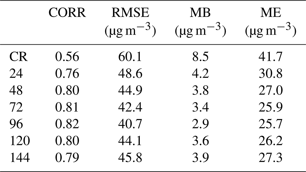
The DA sites were used to assimilate the initial field at 00:00 UTC each day for December 2016, and six different ensemble sizes were used to improve the initial field as shown in Table 4. Compared with the initial field without data assimilation, the RMSE, CORR, MB, and ME of the initial field after assimilation had all been improved, and the improvements were different depending on the ensemble size. The priori initial field is shown in Table 4 CR. With only 24 ensemble samples assimilated, the RMSE of verification sites decreased from 60.1 to 48.6 µg m⁻³, the CORR increased from 0.56 to 0.76, and the MB and ME decreased from 8.5 to 4.2 and 41.7 to 30.8 µg m⁻³, respectively. As seen in Table 3 the statistics of verification sites become progressively better as the ensemble members increase from 24 to 48, 72, and 96. The verification site RMSEs for 48, 72, and 96 samples are 44.9, 42.4, and 40.70 µg m⁻³, respectively; the CORRs are 0.80, 0.81, and 0.82; and the MEs are 27.0, 25.9, and 25.7. When 120 samples or 144 samples were selected for assimilation, the analysis field PM_2.5 DA and verification statistics were not better than those of 96 samples. The verification site RMSEs for 120 and 144 samples were 44.1 and 45.8 µg m⁻³, respectively, and the CORRs also became smaller. The differences between the statistics also indicate there is an optimal ensemble size; the RMSE of the experiment using 96 samples is smaller than the RMSE when using the other ensemble sizes, and the remaining statistics are better than the results when other samples are selected, so we consider that in these sensitivity experiments the best assimilation is achieved when the number of the ensemble size is 96. It is noted from the experimental results that the larger the ensemble does not mean the better the results in this study. It could be influenced by the following reasons: the atmospheric chemistry model used in the study is coupled online with the mesoscale regional weather model GRAPES_Mese5.1. The mesoscale regional weather model differs from the climate model and the global model in that the mesoscale model represents weather systems on timescales of 1 d to several days (Emanuel, 1986). In addition, atmospheric chemical processes are fast-varying processes with small timescales compared to climatic and oceanic processes, so using model results from long time integrations as ensemble may average out the “error of the day” and will not be a very good assessment of model background errors.

Table 4 Statistics of PM_2.5 concentrations for verification sites of the initial field without (CR) and with assimilation at 00:00 UTC each day from 1 to 31 December 2016. Assimilation sensitivity experiments were performed with a localization length scale L of 80 km and an ensemble size of 24, 48, 72, 96, 120, and 144, respectively, and only assimilated the assimilation sites.

3.3 Impact on initial fields

In order to verify the assimilation effect and quantitatively evaluate the impact of the EnOI system on the initial fields, DA experiments with a length scale of L=40 and an ensemble size of N=96 were performed on the initial field at each 00:00 UTC from 15 to 23 December 2016. The assimilated observations were obtained from the DA sites in Fig. 2, and the effect on both DA sites and verification sites were evaluated. Figure 5 shows the statistics for the two regions of the initial field, mainland China and northern China. In mainland China, the CORRs of the verification sites and DA sites before assimilation were 0.60 and 0.58, respectively, and the RMSEs were 73.9 and 73.4 µg m⁻³, respectively. After the DA sites were assimilated, the CORR of assimilated sites increased to 0.99, and the RMSE decreased to 14.5 µg m⁻³, and the CORR of verification sites increased to 0.84 and the RMSE decreased to 46.4 µg m⁻³; meanwhile the ME changed from 49.7 to 27.3 µg m⁻³. In northern China, after the DA sites were assimilated, each statistic of the validation site also changed, with the CORR increasing from 0.53 to 0.87 and RMSE decreasing from 105.5 to 65.7 µg m⁻³. Only 50 % of the ground-based observations are assimilated, and the statistics of the validation sites have also been improved. These experimental results prove that the DA system can indeed yield more accurate initial fields with an over 40 % increase in CORR and 37 % reduction in RMSE.

Table 5 Statistics of initial PM_2.5 concentrations for assimilation sites (DA) and verifications sites (Ve) before EnOI (BF) and after EnOI (AF) at 00:00 UTC on 16, 19, 20, and 23 December 2016, respectively.

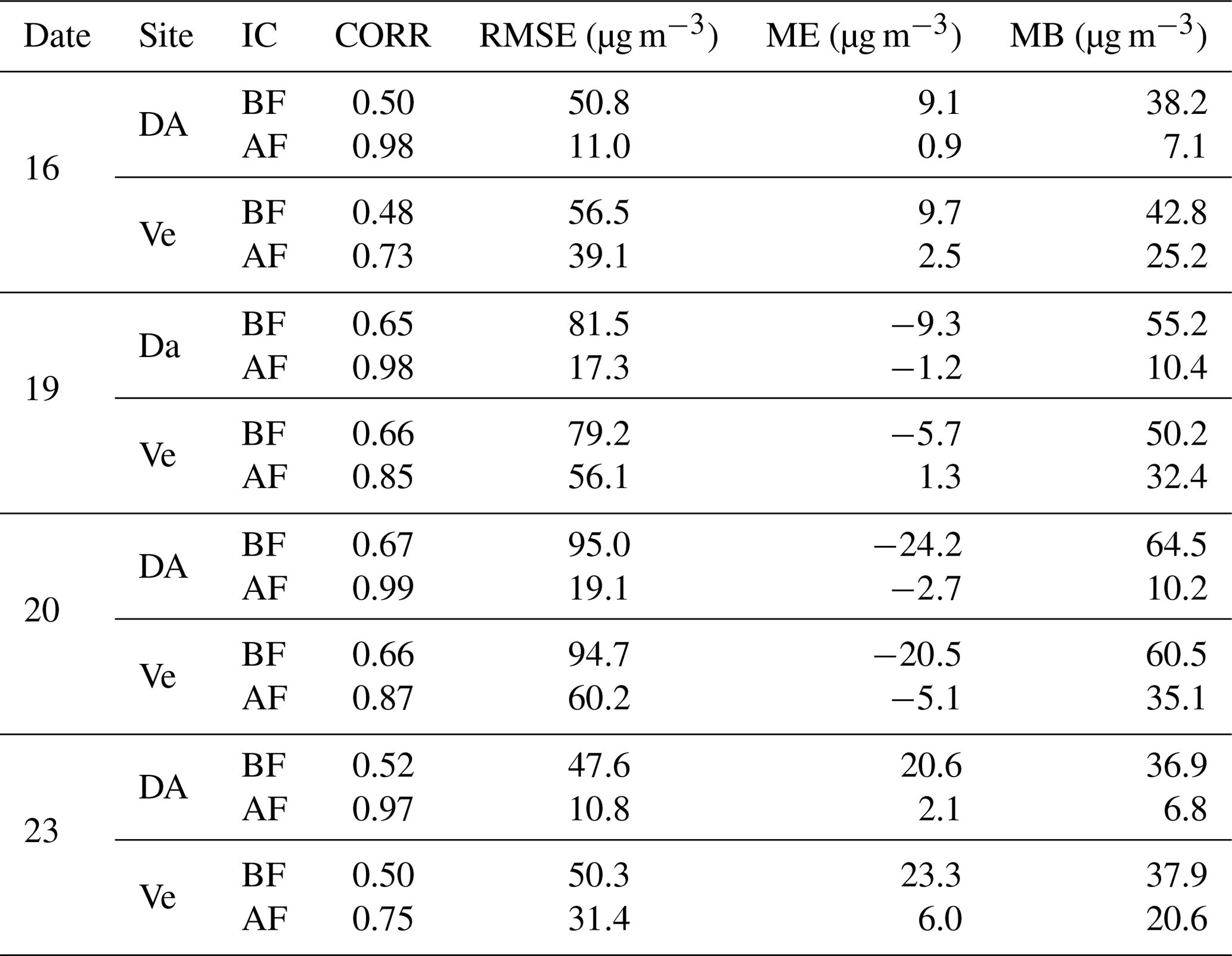
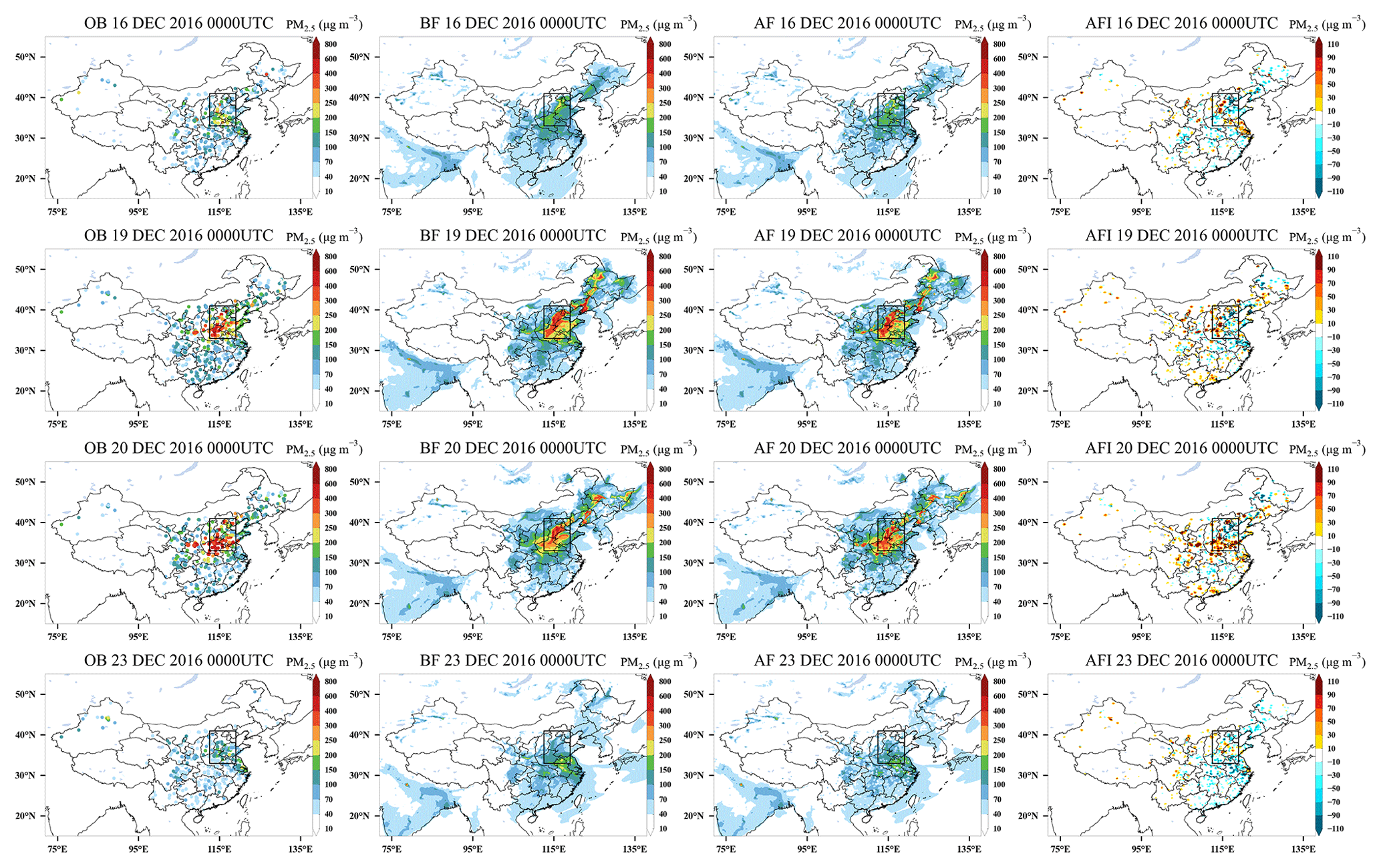
Figure 6 Snapshots of the horizontal distributions of PM_2.5 observation (OB), before (BF) and after (AF) the application of the EnOI technique, and analysis field increment (AFI) at 00:00 UTC on 16, 19, 20, and 23 December 2016. The black box area represents northern China (NC).

To illustrate the assimilation effect of different pollution levels, we consider this episode from 15 to 23 December 2016, where 15 and 16 December is the period of pollution start, 17 to 21 December is the period of pollution, and 22 to 23 December is the period of pollution dissipation. We compared the PM_2.5 observations and initial conditions before and after DA within all the observation sites assimilated during this episode. This was done to understand the impact of DA on initial conditions in the system's actual operating situation. Figure 6 shows the spatial distribution of PM_2.5 in the observation field (OB), background field (BF), analysis field (AF), and analysis field increments (AFIs) for 2 d of light pollution (16 and 23 December) and 2 d of heavy pollution (19 and 20 December). The black boxed area in Fig. 6 is the same as northern China (NC) in Fig. 2, including Beijing, Tianjin, eastern Shanxi, southern Hebei, western Shandong, and northern Henan, which has the highest simulated PM_2.5 concentration. Table 5 summarizes the corresponding statistics of initial PM_2.5 concentrations for assimilation sites and verifications sites before and after EnOI. Figure 6 shows that, compared with OBs, the model background PM_2.5 without DA can capture the spatial pattern of distribution over China in general, which shows that the model performance is moderately good. However, there are still errors between the background and observations. PM_2.5 concentrations are overestimated in NC and eastern China during the pollution start and dissipation periods. During the heavy-pollution period, the background PM_2.5 concentrations are overestimated in northeastern China and underestimated in NC. After assimilating the ground-based PM_2.5, the PM_2.5 concentration increments were distributed around the observation sites as expected and were more closer to the observation distributions. Negative values of the AFI demonstrate that assimilation reduces PM_2.5 concentrations, while positive values demonstrate that assimilation increases PM_2.5 concentrations. During the period before and after pollution, PM_2.5 concentrations decrease in eastern China and increase in western China and NC, indicating a reduction in over- or under-prediction of model PM_2.5 concentrations after assimilation. Table 5 shows that assimilating 50 % of the ground-based observations improved the initial condition for other areas which have no assimilated sites. Take 19 December 2016 as an example; the CORR for verification sites increased from 0.66 to 0.85, RMSE decreased from 79.2 to 56.1 µg m⁻³, and MB and ME also became smaller after EnOI. These results indicate that the initial PM₂₅ fields can be adjusted efficiently by EnOI. What the impact of this innovation through the EnOI system for forecasts is is discussed in the next section.

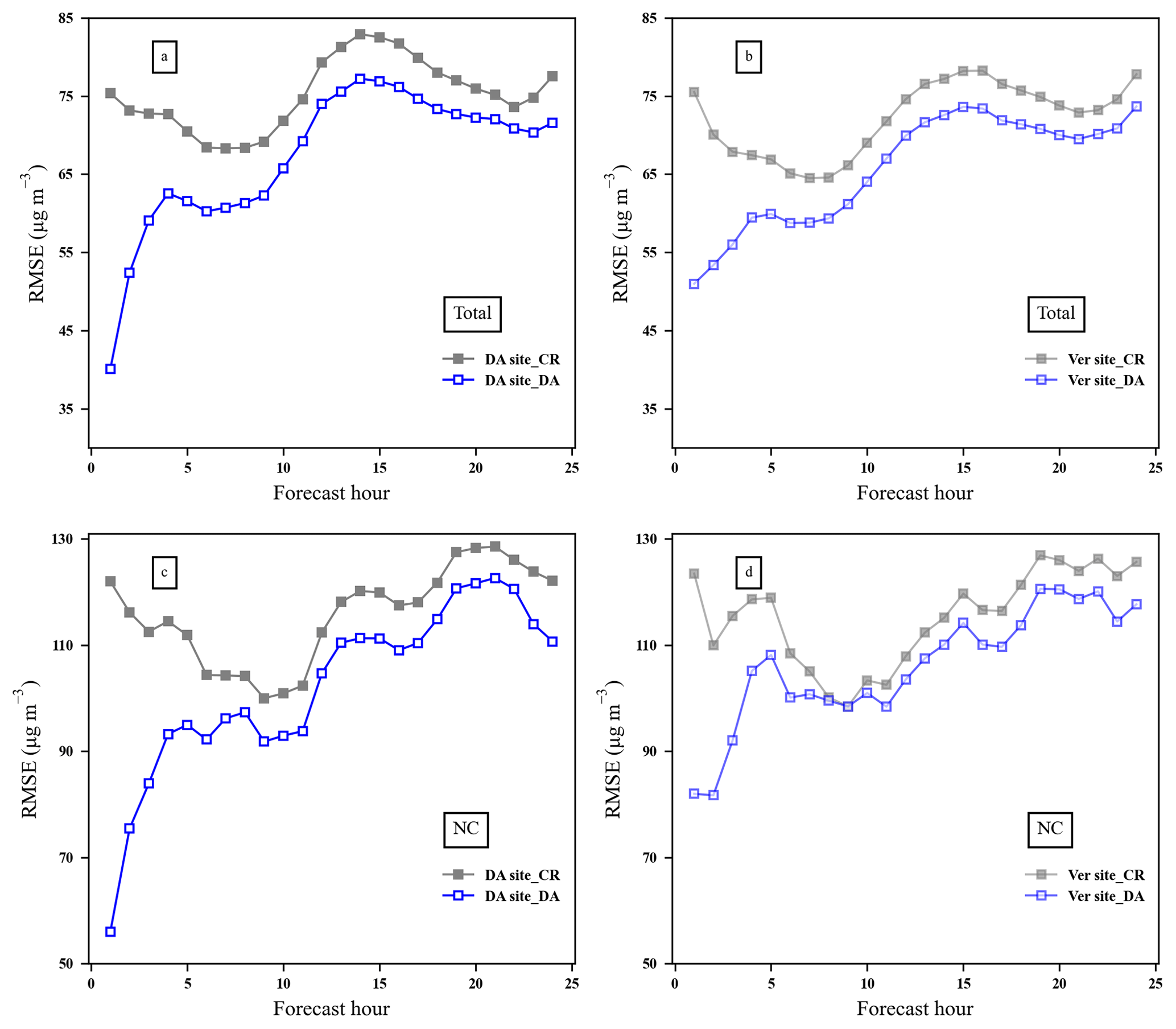
Figure 7 The average RMSE value of surface PM_2.5 forecasts as a function of forecast time over (a) mainland China for DA sites, (b) mainland China for verification sites, (c) northern China for DA sites, and (d) northern China for verification sites.

3.4 Impact on forecast

3.4.1 Impact on PM_2.5 forecast

In this section, we will discuss the impact of assimilation observations on PM_2.5 forecasts. As in Sect. 3.3, we assimilate the DA sites at 00:00 UTC from 15 to 23 December 2016 and then analyse the following forecast of DA and the verification sites separately. The RMSE of the DA and verification sites in mainland China and northern China for a complete pollution-process-obtained average over 15 to 23 December 2016 is shown in Fig. 7. For the DA sites in mainland China (Fig. 7a), the model forecast RMSE without DA is about 75 µg m⁻³; after the assimilation, the model forecast RMSE is decreased rapidly from 75.4 to 40.1 µg m⁻³, which is an over 40 % reduction. This implies that assimilation with EnOI can considerably improve the forecast accuracy. Meanwhile, it is notable that assimilation of DA sites also has an impact on the forecast at the verification sites. The trend of the RMSE series at the verification site is consistent with the DA site but smaller in value. The RMSE of verification sites at a 1 h forecast hour dropped from 75.5 to 51.0 µg m⁻³, about a 32 % reduction. For northern China, which was shown in Fig. 7c and d, the model forecast RMSE without DA is about 115 µg m⁻³. After the assimilation of PM_2.5 observation, the model forecast RMSE of DA sites at the 1 h forecast time is decreased rapidly from 122.0 to 56.1 µg m⁻³, which is an over 54 % reduction. For verification sites, the reduction amplitude is 33 %, smaller than that of DA sites but still a moderate improvement considering only 50 % of ground-based observations were used to be assimilated at 00:00 UTC. The results show that assimilation with EnOI improves the forecast not only for the DA sites but also for the verification sites. The improvements are mainly within the first 12 h forecasts with an RMSE greater than 10 µg m⁻³. The improvement receded with forecast time, changing from 46 % at the 1 h forecast hour to 7 % at the 24 h forecast hour. These results are consistent with previous studies, which used either 4D-Var or EnKF (Skachko et al., 2016; Bocquet et al., 2015; Park et al., 2022). As Bocquet et al. (2015) pointed out, even with the improved analysis, the impact of the initial state adjustment is generally limited to the first day of the forecast, for pollutant transport and transformation are strongly driven by uncertain external parameters, such as emissions, deposition, boundary conditions, and meteorological fields.

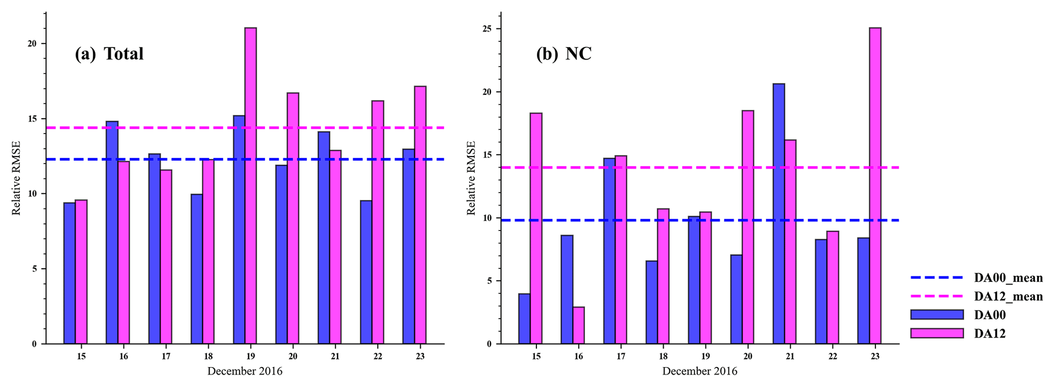
Figure 8 Rate of improvement (ROI; unit: %) by data assimilation in 1 d (24 h) predictions for 15 to 23 December 2016 over mainland China (a) and northern China (b). The ROI is the ratio of the reduced RMSE statistical metrics to those for the CR simulation. DA00 and DA12 represent the initial field assimilation using EnOI at 00:00 and 12:00 UTC each day, respectively. DA00_mean and DA12_mean represent the mean ROI from 15 to 23 December 2016 of DA00 and DA12, respectively.

Now we use all ground-based observation sites as DA sites to investigate the performance of assimilating the initial field at 00:00 UTC each day (DA00) or 12:00 UTC each day (DA12) on improving the PM_2.5 forecasts. DA00 and DA12 were performed in parallel. The daily average of the 24 h RMSE was obtained for the DA and CR experiments. The rate of improvement (ROI) by data assimilation in 1 d (24 h) predictions for 15 to 23 December 2016 for mainland China and NC was calculated using the ratio of the reduced RMSE statistical metrics to those for the CR simulation and was plotted in a daily time series histogram as shown in Fig. 8. In this episode, the improvement of mainland China PM_2.5 forecasts by DA00 and DA12 is minimal at 9 % and 10 %, respectively, on 15 December and maximal at 15 % and 21 %, respectively, on 19 December. The minimum and maximum improvements of assimilation on PM_2.5 forecasts in NC both appear in DA12, which are 4 % and 25 %, respectively. The difference between DA12 and DA00 relative RMSEs is mostly positive, within 6 % in mainland China, but in NC this difference can be up to 15 %. The average RMSE improvement of the 24 h forecast for the mainland China and northern China assimilation at 00:00 UTC is 12.3 % and 9.8 %, respectively, while that at 12:00 UTC is 14.4 % and 14.0 %, respectively. In terms of the average relative RMSE for this episode, assimilating the initial field at 12:00 UTC improves the PM_2.5 forecast more than that at 00:00 UTC, mainly because the model forecasts are not close to the observations at 12:00 UTC in most cases; thus choosing this time for assimilation will have a significant impact. In addition, the DA effect varies for each day, and the larger the error, the greater the improvement in RMSE from DA, which means that the larger the a priori error, the greater the improvement from DA. These results show that using EnOI to assimilate ground-based PM_2.5 observations for the model chemical initial field can reduce over 9.8 % of RMSE for the 24 h forecast on average. Park et al. (2022) implemented an ensemble Kalman filter in the Community Multiscale Air Quality model (CMAQ model v5.1) for data assimilation of ground-level PM_2.5. They found using EnKF with 40 ensemble numbers can reduce 9.6 % of RMSE for a 24 h forecast. Comparing their results with ours, we can find that, while EnOI is suboptimal, it can give an improvement of forecast that is comparable to that of the EnKF. Moreover, the computational cost of EnOI is typically about N times less than that of EnKF. Therefore, we suggest that EnOI may provide a practical and cost-effective alternative to EnKF for the applications where computational cost is the main limiting factor, especially for real-time operational forecast.

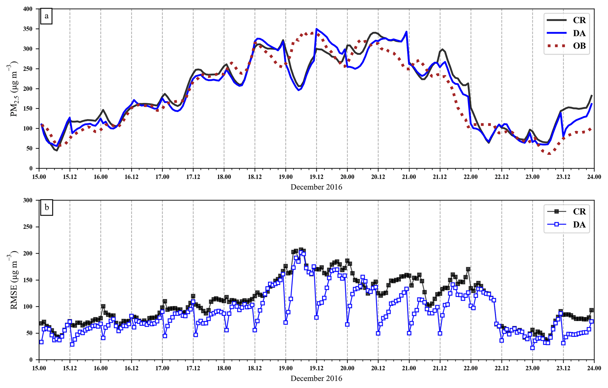
Figure 9 Time series of hourly PM_2.5 concentration (a) and RMSE between forecasts and observations (b) from 15 to 23 December 2016 in northern China. Red dots, observations; black line, forecasts from the control experiment (CR); blue line, forecasts from the experiment with initial field assimilation at 00:00 and 12:00 UTC (DA); black line with dots, RMSE between CR forecasts and observations; blue line with dots, RMSE between CR forecasts and observations. The values are averages calculated against all the observation sites in northern China.

To achieve better performance of assimilation, we update the initial field every 12 h. Figure 9 gives time series of forecasts and observations in terms of PM_2.5, together with RMSE of CR and DA for northern China. Compared with the observations, the forecast PM_2.5 concentrations are 20 to 100 µg m⁻³ higher in the pollution start period (15–17 December) and the pollution fading period (21, 23 December), about 100 µg m⁻³ lower on 19 December. The PM_2.5 concentrations change immediately 1 h after 00:00 or 12:00 UTC. It can be seen from Fig. 9b the RMSEs of the DA experiments are always lower than those of the CR experiments, and the difference in RMSE between the CR and DA experiments recedes with forecast time. This proves that assimilating the initial field can improve the PM_2.5 forecast. Note that the DA algorithm used here cannot produce an optimal solution when there are larger errors in the model. On 19 December 2016, even with DA the model still cannot retrieve the true variation very well for the first 12 h forecast. This suggests that using DA on the initial field can only partially remedy inherent model error. To improve the analysis capabilities and prolong the impact of DA on PM_2.5 forecasts, we should extend the assimilation for adjusting emissions, meteorological fields, and other model uncertainty sources.

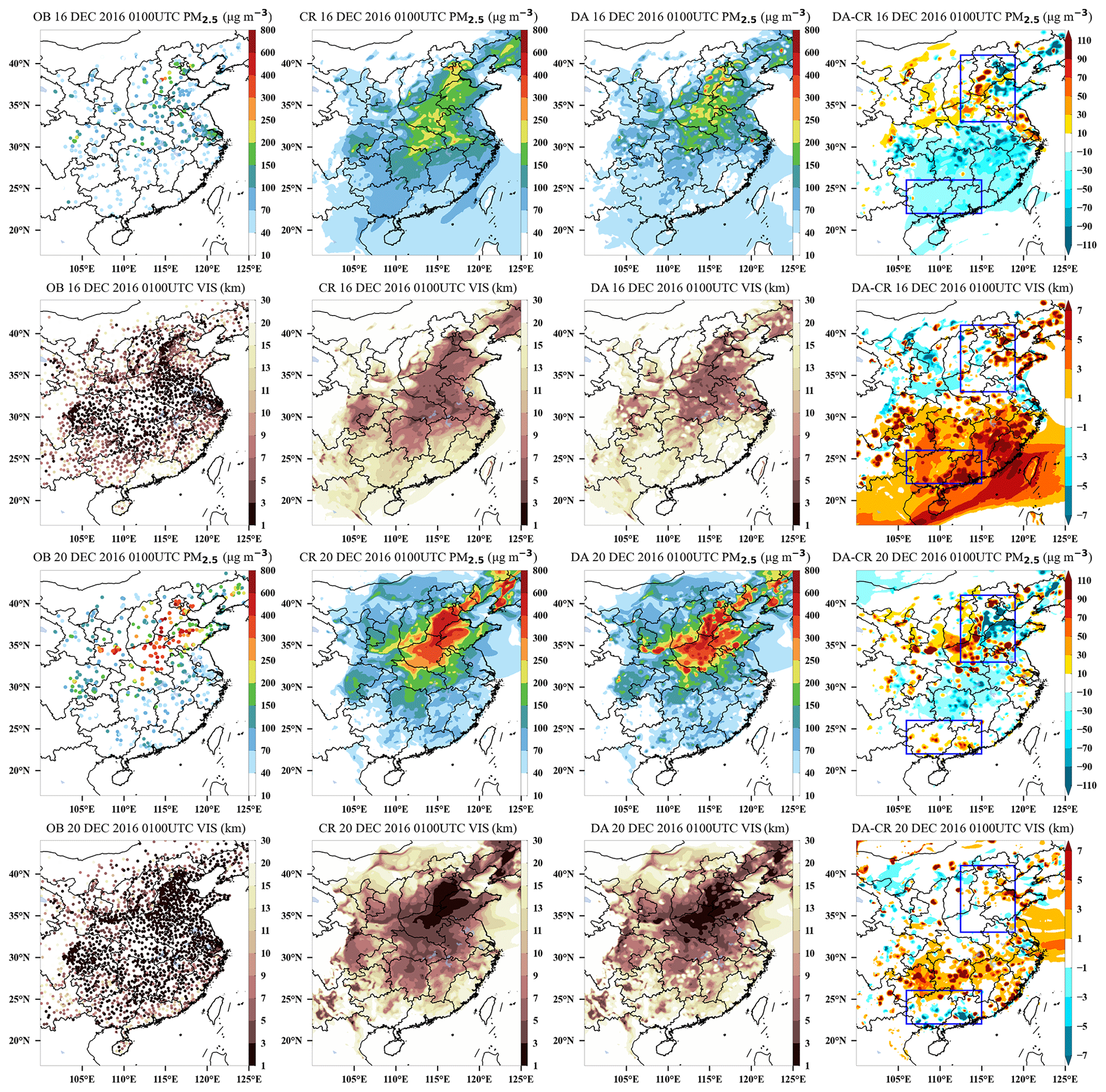
Figure 10 Snapshots of PM_2.5 and visibility horizontal distribution for control (CR), assimilation (DA), observation (OB), and increment (DA–CR) at 01:00 UTC after assimilation of the initial field at 00:00 UTC on 16 and 20 December 2016. The upper box represents northern China, and the lower box represents Guangxi and Hainan in China.

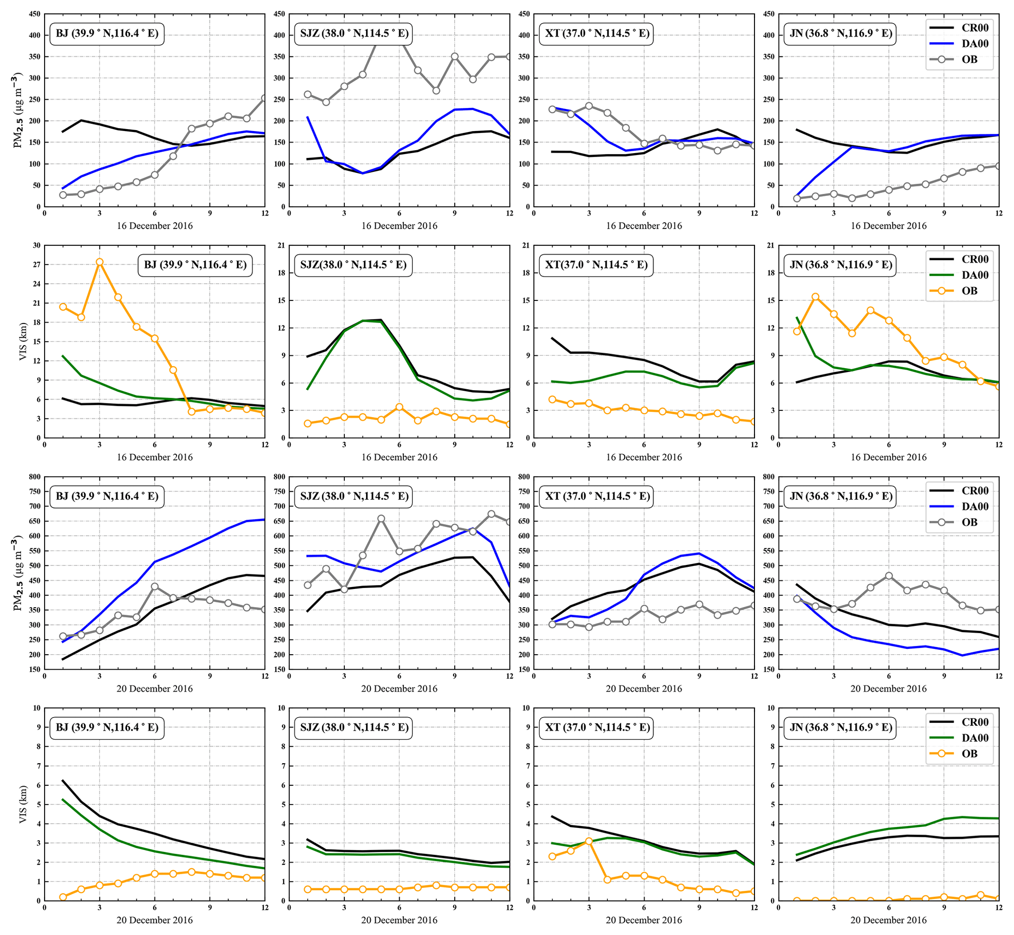
Figure 11 Comparison between PM_2.5 and visibility observations and model forecast at four cities without (CR00) and with assimilation (DA00) of the initial field at 00:00 UTC on 16 and 20 December 2016. The four cities are exemplified, from left to right: Beijing (BJ), Shijiazhuang (SJZ), Xingtai (XT), and Jinan (JN). The labels on the x axis refer to the first 12 forecast hours of the day. PM_2.5 observations, grey line with circles; visibility observations, orange line with circles; PM_2.5 and visibility model forecast without assimilation, black line; PM_2.5 model forecast with assimilation, blue line; visibility model forecast with assimilation, green line.

3.4.2 Impact on visibility forecast

The occurrence of low-visibility episodes is usually associated with aerosol pollution. The horizontal spatial distribution of the OBs, forecast fields without assimilation (CRs), forecast fields with assimilation (DAs), and incremental fields (DA–CRs) for visibility and PM_2.5 at 01:00 UTC on 16 and 20 December are shown in Fig. 10. During the pollution start period (16 December 01:00 UTC) visibility is above 10 km in most of China, and during the pollution period (20 December 01:00 UTC) visibility is mostly below 7 km in eastern China. After assimilating the ground-based PM_2.5, the visibility distribution of DAs is more consistent with the observation compared to the CRs. A positive PM_2.5 concentration increment corresponds to a negative visibility increment, which means that when the PM_2.5 concentration increases, the visibility decreases at the same moment. At 01:00 UTC on 16 December, the CR PM_2.5 concentration is underestimated in NC and overestimated in southeastern China, and after assimilating PM_2.5, the visibility is reduced in NC with increased PM_2.5 and increased in the southeast with reduced PM_2.5. In the period of light pollution, the absolute value of the visibility increment is mostly in the range of 5–7 km when the PM_2.5 increment is from 30 to 110 µg m⁻³ or from −30 to −110 µg m⁻³ in NC, while in the pollution period (20  December 01:00 UTC for example), under the same PM_2.5 analysis increment, the visibility increment in NC is between −3 and 3 km.

Four stations, Beijing (BJ), Shijiazhuang (SJZ), Xingtai (XT), and Jinan (JN), were selected from the heavily polluted NC to study the effect of assimilating the initial field PM_2.5 on the visibility forecasts. Since the assimilation effect is the most obvious in the first 12 h, we focus on the improvement of visibility forecasts within 12 h. Figure 11 shows the observation, simulation, and assimilation of visibility, as well as the observation, simulation, and assimilation of PM_2.5 concentration for the above cities from 01:00 to 12:00 UTC on 16 and 20 December 2016. On 16 December, when the PM_2.5 concentration is less than 300 µg m⁻³ (16 December), visibility at all four stations is closer to the observed value by assimilating PM_2.5, among which BJ and JN have decreased PM_2.5 concentrations after assimilation, and visibility has increased at the same time. SJZ and XT have increased PM_2.5 concentration and decreased visibility after assimilation. In the period of low PM_2.5 concentration, about a 100 µg m⁻³ PM_2.5 change causes a visibility change of 11, 4, 5, and 7 km in BJ, SJZ, XT, and JN, respectively. In the period of heavy pollution, the PM_2.5 concentration changes with 150 µg m⁻³ in Beijing and Shijiazhuang at 01:00 UTC, while visibility changes with 3.5 and 0.5 km, respectively. These results show that the improvement of visibility by assimilating PM_2.5 is limited during the heavy-pollution period. It is worth noting that when the PM_2.5 concentration is greater than 350 µg m⁻³ at the JN site, although the decrease in PM_2.5 concentration corresponds to the increase in visibility, the gap between the assimilated visibility and observation becomes larger at this time, which may be related to the inaccuracy of the humidity simulation here and inaccurate visibility parameterization scheme for the model. Visibility is not linearly related to PM_2.5, and visibility is also affected by humidity and other factors. Assimilation of the initial field PM_2.5 can improve the visibility forecast, but if we want to improve the visibility forecast significantly, we need to improve not only the visibility parameterization scheme, but also the humidity accuracy. The present study focuses on data assimilation of chemical initial fields and is the first step of implementation of EnOI for a regional online chemical weather numerical forecasting system. Next, the uncertainty in the emissions as well as physical and chemical parameterization should also be considered. Moreover, the joint assimilation of meteorological and chemical variables and feedbacks between chemistry and meteorology are worthwhile to be investigated in future studies.

4 Conclusions

To improve the accuracy of PM_2.5 and visibility forecasting in China, a real-time and efficient EnOI assimilation system is established for the latest online operational chemistry weather model GRAPES_Meso5.1/CUACE of the China Meteorological Administration. The surface PM_2.5 observation data from nearly 1500 ground stations across the country are used for assimilation. PM_2.5 and visibility simulation–assimilation experiments were performed for a haze pollution episode from 15 to 23 December 2016. Parallel sensitivity experiments of a localization length scale and an ensemble size were set up to determine two key parameters that influence the effectiveness of the EnOI assimilation. Based on the results of the sensitivity experiments, the initial fields were assimilated at 00:00 UTC each day from 15 to 23 December 2016 to study the improvement of EnOI on the initial field PM_2.5. In addition to the analysis of the mainland China assimilation effect, the heavily polluted northern China region was additionally divided to discuss the different impacts of assimilation on the overall and regional chemical initial fields. Cyclic assimilation experiments were performed at 00:00 (DA00) and 12:00 UTC (DA12) to investigate the impacts of assimilation on the forecast fields, taking NC as an example, to discuss the impacts of assimilation on PM_2.5 and visibility forecast fields.

The optimal localization length scale and the number of ensemble samples are 40 km and 96, respectively, derived from sensitivity experiments. Assimilating 50 % of the ground-based observations improved the initial condition for other areas which have no assimilated sites. The DA considerably improved the model PM_2.5 initial field, the CORR of verification sites in mainland China improved from 0.58 to 0.84, and the RMSE decreased from 73.7 to 46.4 µg m⁻³. The results of the DA00 and DA12 assimilation experiments showed that the improved impacts of the DA worked throughout the forecast time window, but the assimilation impact was the most pronounced in the first 12 h and gradually decreased in the subsequent time. Within the 24 h forecast time window, the average RMSE improvement for the mainland China PM_2.5 forecast field ranges from 9 % to 21 % and between 4 % and 25 % in NC, and the comprehensive comparison shows that the initial field of the 12:00 UTC assimilation is superior to 00:00 UTC. Therefore, in this study, it is considered that with limited computational resources, the EnOI assimilation efficiency is the highest with the largest distance between the model simulation and observation to assimilate according to the model characteristics. When it comes to operational use, the assimilation efficiency can be improved by shortening the assimilation time interval due to the small demand of EnOI computational resources.

The assimilation of PM_2.5 also has a positive impact on visibility forecasts. When the PM_2.5 increment by assimilation is negative, it corresponds to an increase in visibility, and when the PM_2.5 analysis increment is positive, visibility decreases correspondingly. The greater the change in PM_2.5 concentration during periods of light pollution, the more pronounced the improvement in visibility. It is worth noting that visibility is also related to a variety of factors, and assimilating only ground-based PM_2.5 sites has a limited effect on visibility, and we will further consider assimilating PM₁₀, humidity, and other meteorology factors to improve visibility forecasts in subsequent studies.