the Creative Commons Attribution 4.0 License.
the Creative Commons Attribution 4.0 License.
 | 24 Jul 2023
An optimized semi-empirical physical approach for satellite-based PM2.5 retrieval: embedding machine learning to simulate complex physical parameters
Caiyi Jin
Tongwen Li
Yuan Wang
Liangpei Zhang
Satellite remote sensing of PM2.5 (fine particulate matter) mass concentration has become one of the most popular atmospheric research aspects, resulting in the development of different models. Among them, the semi-empirical physical approach constructs the transformation relationship between the aerosol optical depth (AOD) and PM2.5 based on the optical properties of particles, which has strong physical significance. Also, it performs the PM2.5 retrieval independently of the ground stations. However, due to the complex physical relationship, the physical parameters in the semi-empirical approach are difficult to calculate accurately, resulting in relatively limited accuracy. To achieve the optimization effect, this study proposes a method of embedding machine learning into a semi-physical empirical model (RF-PMRS). Specifically, based on the theory of the physical PM2.5 remote sensing (PMRS) approach, the complex parameter (VEf, a columnar volume-to-extinction ratio of fine particles) is simulated by the random forest (RF) model. Also, a fine-mode fraction product with higher quality is applied to make up for the insufficient coverage of satellite products. Experiments in North China (35∘–45∘N, 110∘–120∘E) show that the surface PM2.5 concentration derived by RF-PMRS has an average annual value of 57.92 µg m−3 vs. the ground value of 60.23 µg m−3. Compared with the original method, RMSE decreases by 39.95 µg m−3, and the relative deviation is reduced by 44.87 %. Moreover, validation at two Aerosol Robotic Network (AERONET) sites presents a time series change closer to the true values, with an R of about 0.80. This study is also a preliminary attempt to combine model-driven and data-driven models, laying the foundation for further atmospheric research on optimization methods.
- Article
(9226 KB) - Full-text XML
- BibTeX
- EndNote


Epidemiological studies have indicated that PM2.5 (fine particulate matter with an aerodynamic equivalent diameter no greater than 2.5 µm) can adversely affect human health, such as increasing the risk of diabetes and respiratory diseases (Bowe et al., 2018; Pope III et al., 2002; Xu et al., 2013), and accurate surface PM2.5 concentration is the basis of air pollution health-related research. Satellite remote sensing has the advantages of high resolution and global coverage (Ma et al., 2014; Wu et al., 2020; He et al., 2022), including variables strongly associated with PM2.5 such as aerosol optical depth (AOD). Therefore, it has become a mainstream method for fine-particle estimation (Zhang et al., 2021).
There are three main satellite-based ways of retrieving PM2.5.
-
Chemical transport models-based method.
This method calculates a scaling factor η between AOD and PM2.5 simulated by atmospheric chemical transport models (CTMs) (Lyu et al., 2022; Xiao et al., 2022) and then transfers the proportional relationship to satellite AOD data when calculating surface PM2.5 concentration (Geng et al., 2015; Van Donkelaar et al., 2006). However, the assumption of a constant factor between simulated and observed values has large spatiotemporal limitations.
-
Univariate/multivariate regression.
This kind of data-driven method establishes a statistical model between AOD, auxiliary variables, and ground PM2.5 observations. Machine learning is a common tool for such regression methods due to its powerful nonlinear fitting ability between multiple variables (Irrgang et al., 2021), but the regression algorithms in machine learning are affected by the distribution and density of ground stations (Gupta and Christopher, 2009; Li et al., 2017).
-
Semi-empirical physical approach.
Taking the physical theory as the basis, surface PM2.5 is derived through an empirical formula constructed from AOD and some PM-related key parameters, including an important empirical parameter related to the optical properties (S). The process steps are explicit and independent of ground station observations. Meanwhile, this approach has stronger physical interpretability than the previous two methods with a large space for optimization.
Due to the complexity of the physical parameters, many studies have optimized the semi-empirical physical approach. Based on 355 nm band radar observations, Raut and Chazette (2009) introduced a specific extinction cross-section to simplify the expression of S, and PM2.5 concentration was estimated. Kokhanovsky et al. (2009) constructed a particle-effective radius model, which can obtain the particle concentrations throughout the atmospheric column. Furthermore, Zhang and Li (2015) proposed the physical PM2.5 remote sensing (PMRS) method. It replaced S by defining a volume-to-extinction ratio of fine particles (VEf) and used a quadratic polynomial of fine-mode fraction (FMF) to simulate VEf, showing certain advantages (Li et al., 2016; Zhang et al., 2020).
However, the above semi-physical empirical models have some shortcomings. Firstly, the satellite data used in the models are blocked by clouds and fog in some areas; thus high-coverage and high-precision products need to be excavated and applied. Secondly, there are still large uncertainties in estimating physical parameters (such as a simple polynomial fit to S in the PMRS method), and their expressions need to be improved. To date, machine learning (ML) has developed rapidly (He et al., 2021). It can detect complex nonlinear relationships of multiple data and model their interaction (Yuan et al., 2020; Lee et al., 2022). This provides an idea for improving the accuracy of physical parameter acquisition so as to estimate high-precision PM2.5 through semi-physical empirical models.
According to this idea, our study proposes an optimized semi-empirical physical model (RF-PMRS) based on the PMRS theory, which attempts to explore the possibility of combining physical models and ML. To be specific, we creatively embed ML (the random forest model) into the PMRS method to simulate the physical parameter (i.e., VEf) derived from FMF and related variables, thus optimizing the previous polynomial expression. Moreover, to further improve the PM2.5 retrieval accuracy, the physical–deep learning FMF (Phy-DL FMF) dataset generated by a hybrid retrieval algorithm of ML and physical mechanisms is introduced. Ultimately, we comprehensively validate the performance of the PM2.5 obtained by our optimized approach.
The remainder of our article is as follows. Section 2 describes the experimental datasets. Section 3 illustrates the specific derivation process of the proposed method. Section 4 analyzes the evaluation results. Some supporting experiments are discussed in Sect. 5. The final part provides the conclusion.
2.1 AERONET data
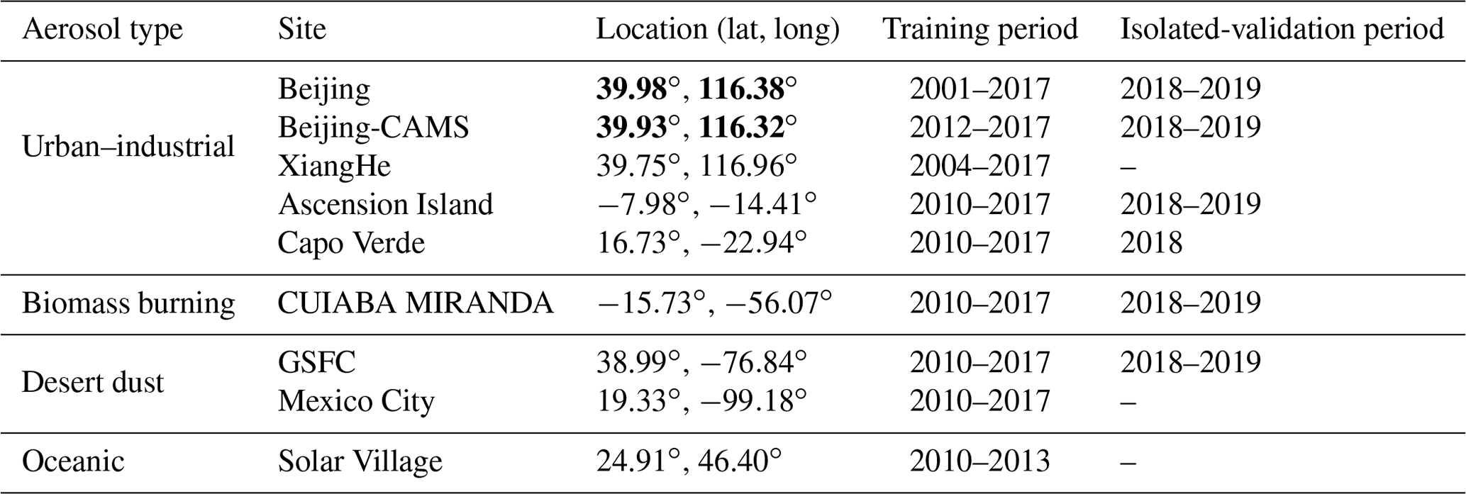
The Aerosol Robotic Network (AERONET) is a federation of ground-based sun–sky radiometer networks, providing worldwide remote sensing aerosol data for more than 25 years (Holben et al., 1998). The current revision of the dataset is Version 3 (Giles et al., 2017). Due to its high quality, the data from AERONET have been regarded as theoretical true values to evaluate satellite-based products in related studies (Chen et al., 2020; Gao et al., 2016; Wang et al., 2019). AOD, FMF, and volume size distribution products with Level 2.0 (quality-assured) are applied to calculate the true values of the physical parameters and then to implement our modeling purpose (not involved in PM2.5 calculations). A total of nine AERONET sites corresponding to four typical aerosol types participate in the training. Table 1 shows the specific information.
Table 1Data information on nine AERONET sites classified by aerosol types. Location indicates the latitude and longitude, where a negative number means a southern latitude and a western longitude. Two sites in bold font participate in the PM2.5 validation experiment. GSFC: Goddard Space Flight Center.
2.2 MODIS AOD
MCD19A2, the Moderate Resolution Imaging Spectroradiometer (MODIS) Collection 6 Level 2 gridded (L2G) land AOD product (Lyapustin and Wang, 2015), is selected in this study. It is derived from the Multi-Angle Implementation of Atmospheric Correction (MAIAC) algorithm, which can improve the accuracy of cloud detection and aerosol retrieval (Lyapustin et al., 2011). Moreover, this new advanced algorithm jointly combines MODIS Terra and Aqua into a single sensor (Lyapustin et al., 2014). The product is produced daily with a 1 km resolution, including aerosol parameters such as 470 and 550 nm AOD, quality assurance (QA), and uncertainty factors.
The processing of MCD19A2 data (in Hierarchical Data Format, HDF) is mainly divided into five steps: AOD–QA band extraction, best-quality AOD selection, Terra–Aqua data synthesis, missing information reconstruction, and mosaic. Finally, the daily AOD distribution in GeoTiff format is obtained.
2.3 Phy-DL FMF dataset
The original global land FMF products have poor data integrity and low accuracy. To enhance their reliability, Yan et al. (2022) have released a satellite-based dataset called Phy-DL FMF, which integrates physical and deep learning methods. Specifically, it selects the FMF data obtained by a physical method (i.e., lookup-table-based spectral deconvolution algorithm, LUT-SDA) as the optimization target (Yan et al., 2017). Then it combines the Phy-based FMF into a deep learning model along with multiple auxiliary data such as satellite observations for the final Phy-DL results. Note that the process is trained with AERONET data as the ground truth. The product has a spatial resolution of 1∘ and covers 2001 to 2020 (daily scale). In the comparison experiment against the ground FMF, Phy-DL FMF shows a higher accuracy (R=0.78, RMSE =0.100) than MODIS FMF (R=0.37, RMSE =0.282) (Yan et al., 2022).
2.4 Meteorological data
The meteorological data are obtained from the ERA5 dataset, including the values of planetary boundary layer height (PBLH) and relative humidity (RH). As the fifth-generation reanalysis product released by the European Center for Medium-Range Weather Forecasts (ECMWF), ERA5 provides atmospheric data at 0.25∘ every hour based on the data assimilation principle (Hersbach et al., 2018). It should be noted that RH is not archived directly in ERA5 and thus should be calculated by 2 m temperature T and dew point temperature Td (refer to https://confluence.ecmwf.int/display/CKB/ERA-Interim:+documentation#ERAInterim:documentation-Computationofnear-surfacehumidityandsnowcover, last access: 20 July 2023):
where es(t) represents the saturation vapor pressure related to a temperature t in degrees Celsius (Simmons et al., 1999) of
2.5 Ground PM2.5 measurements
The North China (NC) region is chosen as the main experimental validation area for the final PM2.5 calculations. The near-surface hourly PM2.5 values are obtained from the China National Environmental Monitoring Centre (CNEMC). Nowadays, over 1600 ground-based monitors are working continuously and a total of 232 stations (in 2017) participate in this work. Figure 1 displays the site distributions of the NC region.
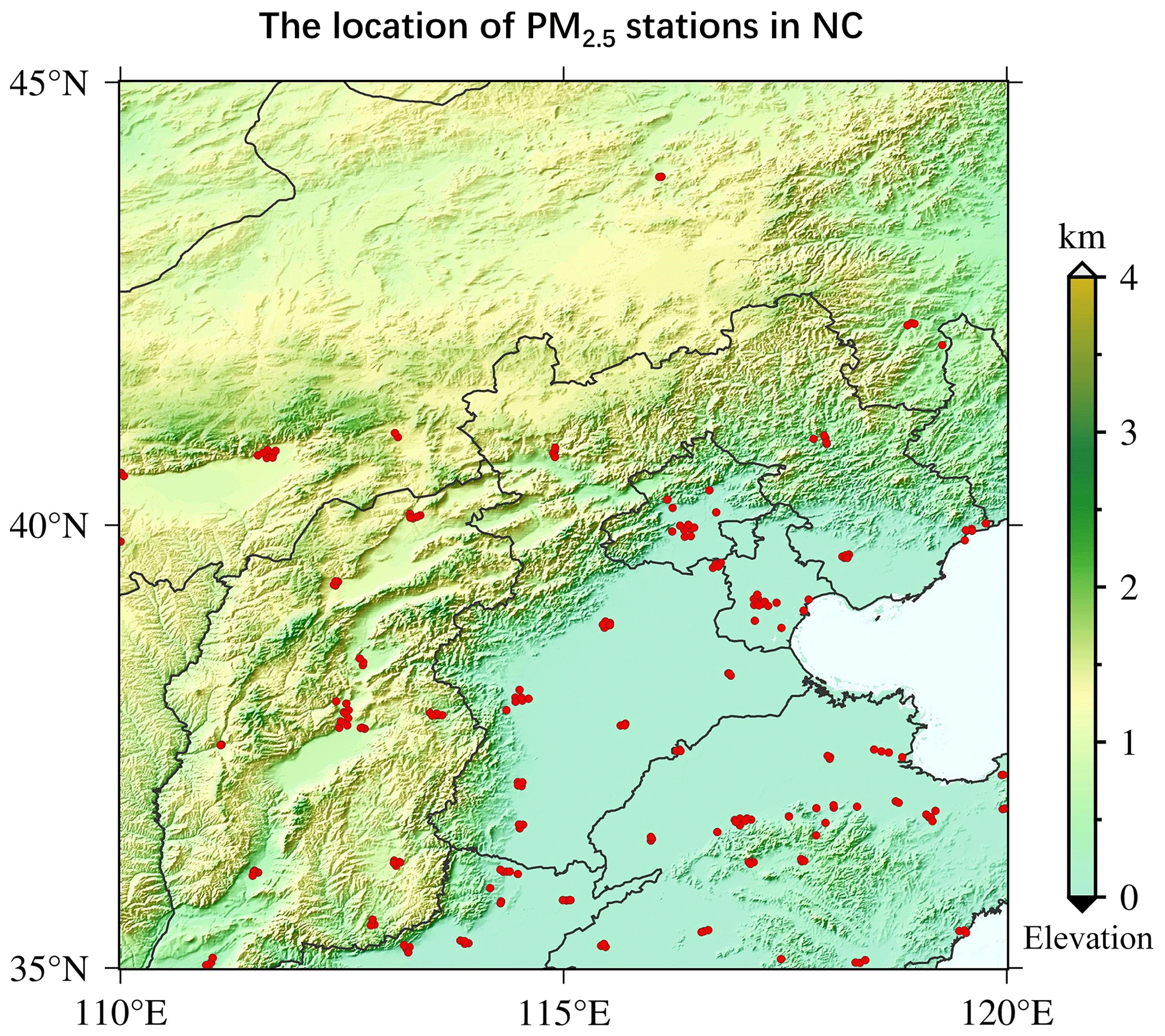
Figure 1The location of PM2.5 ground monitoring stations in the NC region (35–45∘, 110–120∘). The red points represent the PM2.5 stations.
Based on the basic physical properties of atmospheric aerosols, the semi-physical empirical approach starts from the integration of PM mass concentration and AOD. Then it combines several key factors related to PM2.5 to derive the in situ PM2.5 concentration through multiple remote sensing variables (Koelemeijer et al., 2006). The overall empirical relationship can be represented as
where ρ denotes the particle density and H denotes the atmospheric boundary layer height. f(RH) represents the hygroscopic growth factor related to relative humidity (RH). S is an optical characteristic parameter that should be simulated.
3.1 PMRS method
3.1.1 The expression of VEf
To illustrate S more precisely, PMRS defines the columnar volume-to-extinction ratio of fine particles (i.e., VEf), which can be regarded as the basis of our optimization method. So Eq. (3) is transformed into
Related to particle size, aerosol extinction, and other properties, VEf can be expressed as
where AODf is the fine-particle AOD and FMF is the fine-mode fraction. Vf,column can be expressed by the vertical integral of particle volume size distributions (PVSDs) within a certain aerodynamic diameter range of
where Dp,c represents the cutting diameter, the empirical value of 2.0 µm is chosen based on previous literature (Hand and Kreidenweis, 2002; Hänel and Thudium, 1977), and V(Dp) represents the PVSD corresponding to the geometric equivalent diameter (Dp).
3.1.2 Specific process and limitations
The PMRS method is developed from Eq. (4). Based on satellite AOD, the near-surface PM2.5 can be obtained through multistep transformation. Figure 2a shows its specific process. Each arrow refers to a step, respectively, size cutting (output: AODf), volume visualization (output: Vf,column), bottom isolation (output: Vf, fine-particle volume near the ground), particle drying (output: Vf,dry, dry Vf), and PM2.5 weighting. The overall expression is as follows:
where FMF denotes the fine-mode fraction, ρf,dry denotes the dry mass density of PM2.5, and PBLH represents the planet boundary layer height. f0(RH) represents the approximation of f(RH) in Eq. (4), as expressed in Eq. (8). Considering the aerosol types in different regions, PMRS fits VEf to a quadratic polynomial relation of FMF (Zhang and Li, 2015):
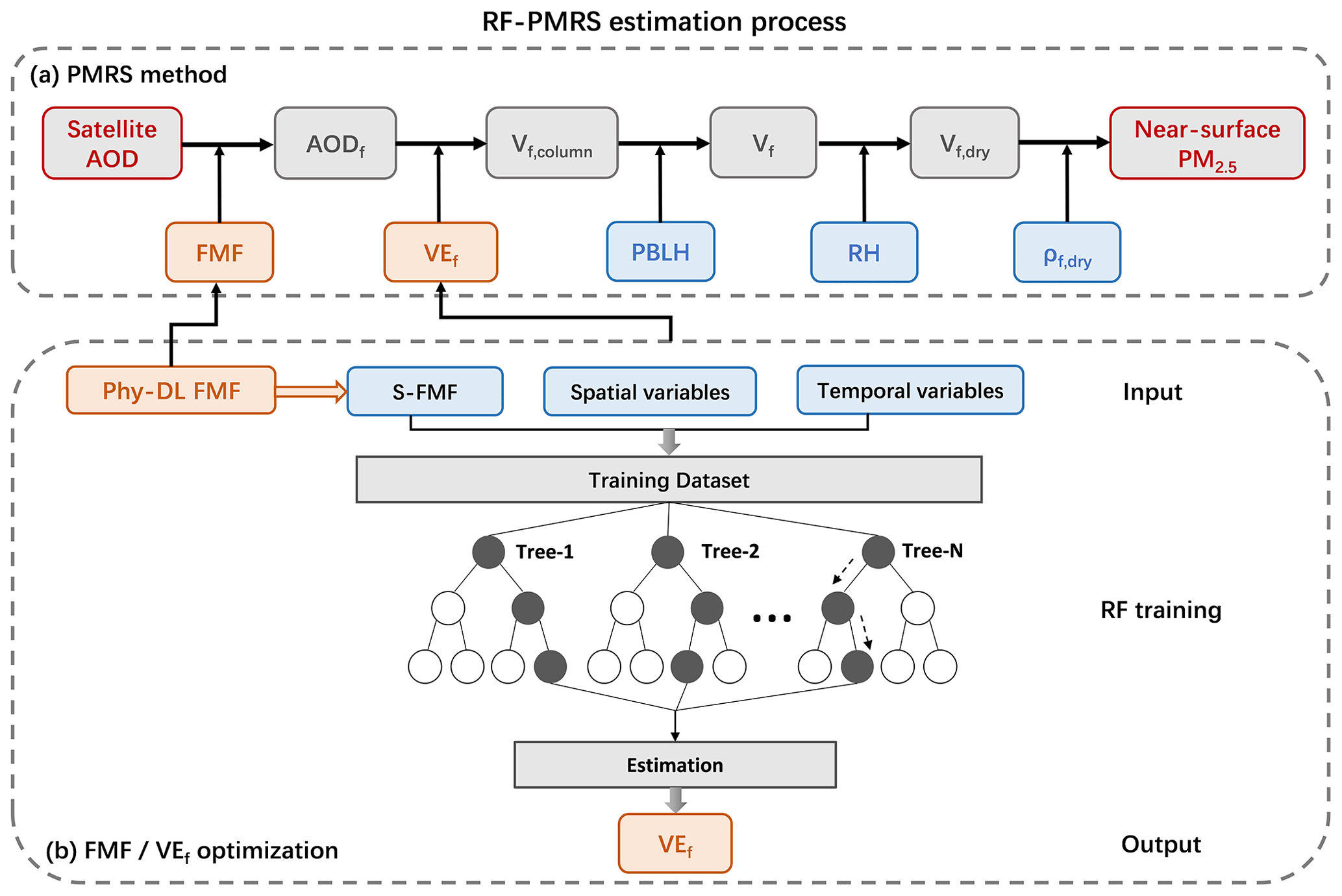
Figure 2Surface PM2.5 estimation flow of RF-PMRS. (a) The five steps of the PMRS method. Gray boxes are the intermediate outputs, blue boxes are the input data, and orange boxes denote the variables to be optimized. (b) The specific optimization of RF-PMRS: FMF dataset replacement and VEf simulation by the RF model.
PMRS has strong physical significance; the calculation steps are well-defined and site-independent. Zhang and Li (2015) tested the performance of PMRS on 15 stations, and the validation results had an uncertainty of 34 %. Compared with the ground value of the city of Jinhua in China, a 31.3 % relative error was generated in Li et al. (2016). Moreover, Zhang et al. (2020) applied it to the PM2.5 change analysis and prediction experiments in China over 20 years. However, there may be a more complex nonlinear relationship between VEf and FMF, not just a simple quadratic formula. Since VEf is related to the aerosol type, adding other spatiotemporal variables may optimize the fitting process. Additionally, high-quality FMF data are the basic guarantee for the estimated PM2.5 quality. In a word, to further improve the physical method, a better nonlinear model between VEf and related variables from reliable datasets needs to be explored.
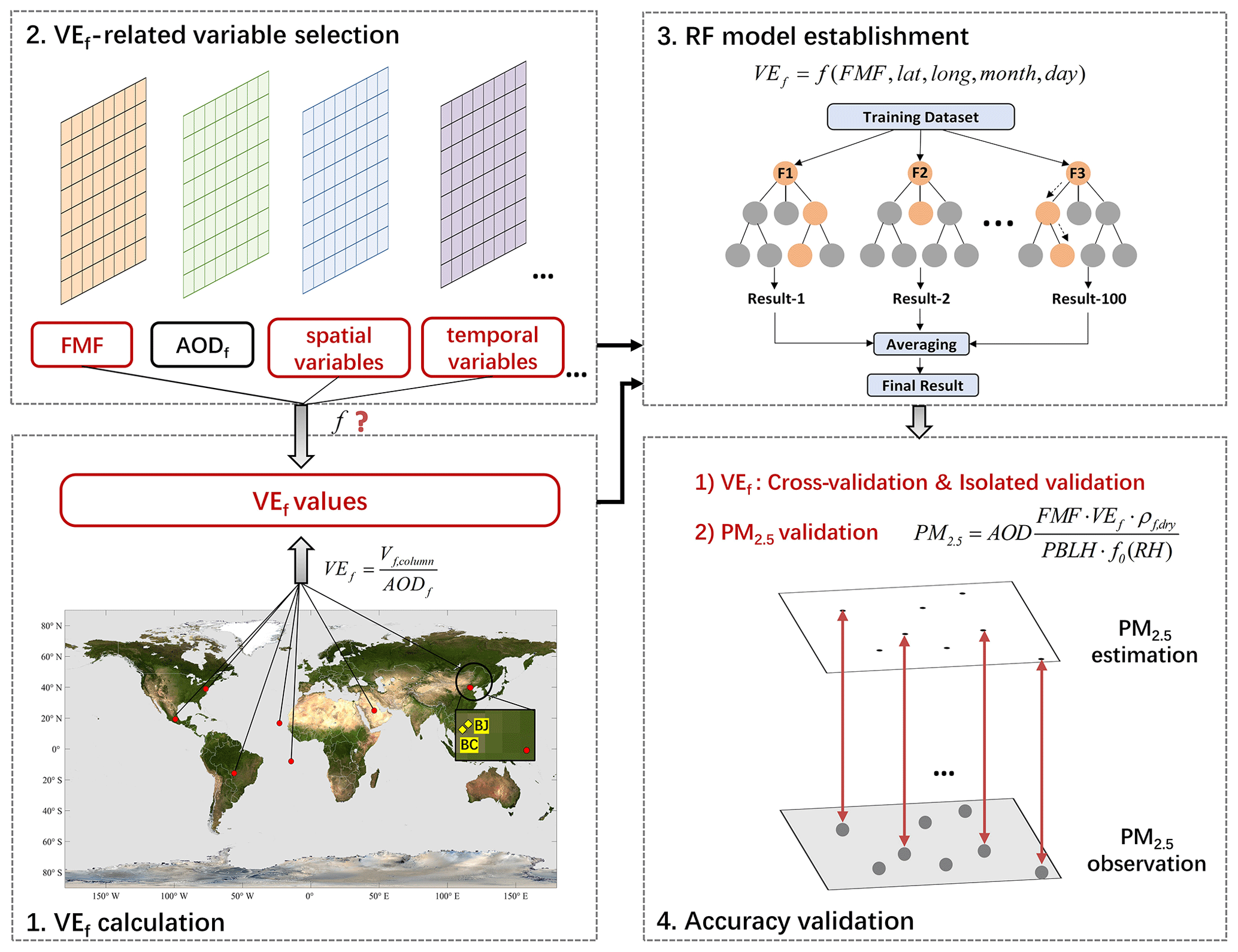
Figure 3Specific steps for simulating VEf based on ML in our RF-PMRS method. The map used in step 1 is from NASA Visible Earth (https://visibleearth.nasa.gov/images/57752/blue-marble-land-surface-shallow-water-and-shaded-topography, last access: 15 June 2023). The red points in step 1 represent the distribution of the nine AERONET sites, and the two yellow quadrangles in the zoom-in view highlight the Beijing (BJ) and Beijing-CAMS (BC) sites.
3.2 Optimization method: RF-PMRS
Therefore, to overcome the above disadvantages, an optimized method called RF-PMRS is proposed. Figure 2b shows the process of our method, while optimizations for FMF and VEf are described separately below.
-
FMF dataset selection.
We introduce the Phy-DL FMF dataset into the PMRS method to improve the accuracy of size-cutting results. In terms of performance, it exhibits higher accuracy and wider space–time coverage than satellite products (Yan, 2021). See the Data section for details.
-
VEf simulation based on ML.
The main idea is to establish an ML model between the VEf truth obtained from multiple AERONET sites and related variables, thus improving the subsequent VEf simulation accuracy (Fig. 3).
-
Step 1: VEf calculation.
The VEf true values are calculated concerning Eqs. (5)–(6). Due to the spatiotemporal variability in different aerosol types, we calculate the VEf values at nine AERONET stations around the world (Table 1) to train a universal model. The first step in Fig. 3 shows their distribution characteristics. Among them, Beijing and Beijing-CAMS sites are highlighted since they participate in the subsequent point validation experiment.
-
Step 2: VEf-related variable selection.
According to the theory, FMF is selected as the most important modeling variable. Previous studies have also shown that the FMF–VEf relationship has a good single-value correspondence, which is not affected by AOD. Compared with AODf and Vf,column, FMF is a better indicator for estimation (Zhang and Li, 2015). In addition, considering the spatiotemporal heterogeneity of VEf, the latitude (lat), longitude (long), and data time (month, day) of each site are added to the training.
-
Step 3: RF model establishment.
From step 2, VEf can be expressed as
We optimize the VEf expression based on the random forest (RF) algorithm. RF is made up of multiple decision trees that can build high-accuracy models based on fewer variables (Ho, 1995; Yang et al., 2020). This ensemble ML method randomly samples the training dataset to form multiple subsets, and random combinations of features are selected in node splitting (Belgiu and Drăguţ, 2016). The specific process is to (1) generate training subsets, (2) build an optimal model, and (3) calculate the result (Fig. 3 shows its flowchart). Note that the station FMF values (S−FMF) from AERONET sites are used when training.
-
Step 4: accuracy validation.
The VEf estimation is also based on Eq. (10), where f is the optimal relationship after RF parameter adjustment, and Phy-DL FMF is applied to realize the extension of model results from the point to the surface. A 10-fold cross-validation (CV) (Rodriguez et al., 2009) and isolated validation (IV) are used to evaluate model performance (for details of the validation methods, see Appendix A1).
-
-
PM2.5 value estimation and evaluation
Then, we calculate PM2.5 according to the corresponding process (Eq. 7). The variables (in Sect. 2.2 to 2.4) are spatially matched to ground sites at their respective resolutions. Based on UTC, the PM2.5 validation is conducted on a daily scale in 2017. Because of the effective quantity of the AERONET public dataset and MODIS data, we choose 2017 as the representative year. Note that we select the measured empirical value of ρf,dry (i.e., 1.5 g cm−3) for the NC region from Gao et al. (2007).
The statistical indicators used in the evaluation include the correlation coefficient (R), mean bias (MB), relative mean bias (RMB), root mean square error (RMSE), and mean absolute error (MAE). In addition, the relative predictive error (RPE) is added to validate the accuracy of the RF-based VEf model. See Appendix A2 for specific information on these indicators.
Three main experiments are conducted to verify the proposed RF-PMRS method, and the specific information is shown in Table 2.
Table 2A brief information summary of the experiments conducted in our study.
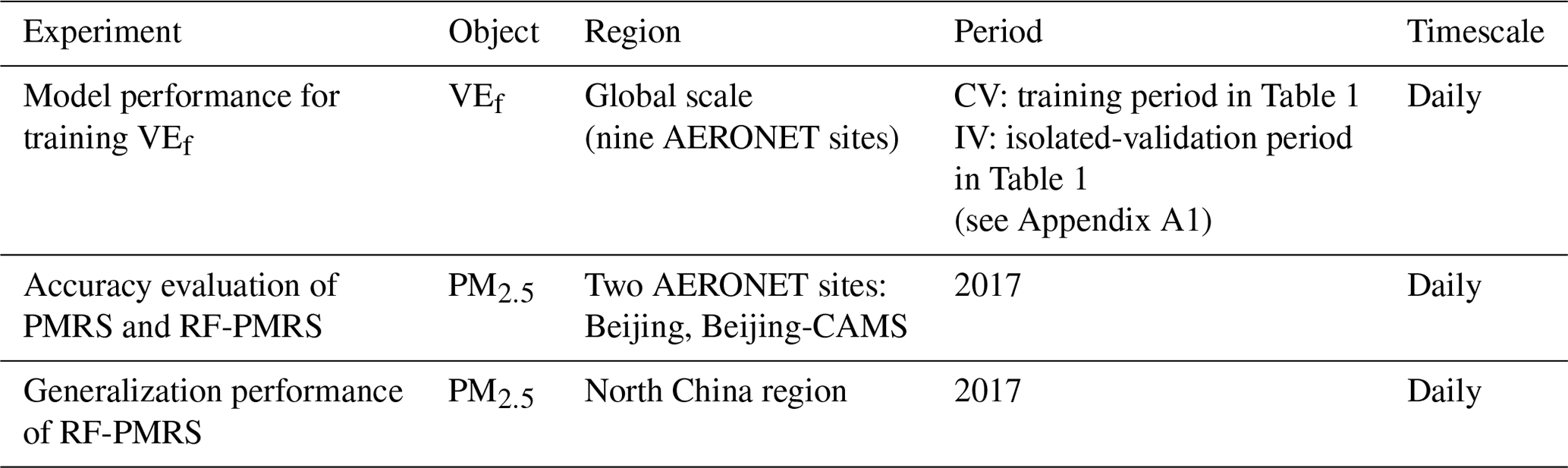
Table 3Performance statistics of the RF model for training VEf. N represents the number of data, and VEf has no unit.

4.1 RF model performance for training VEf
The simulation model of VEf is trained based on the data in Table 1. Specifically, the 10-fold CV result is used to determine the optimal combination of parameters for the model (see Appendix A3 for the adjustment of the model parameters). Considering that the completeness of the training data will optimize the generalization performance of the model, the experiment fine-tunes the model based on all the original datasets (the training period of Table 1) under the optimal parameters, and then the final RF model is constructed. This is also the most common method for ML model construction. Next, the IV experiment provides independent time validation of the final model.
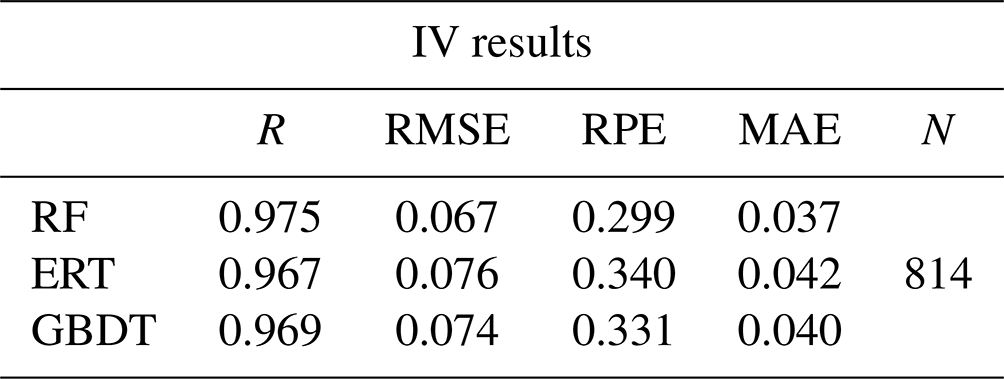
Table 3 shows the CV and IV results to, respectively, demonstrate the internal and external accuracy of the final RF model. It can be seen that RF can capture the complex relationship between VEf and related variables well. R is as high as 0.974 (0.975), RMSE and MAE are both small, and RPE is around 30 %, which suggests the desired estimation accuracy. Overall, the CV results represent the great performance of the RF model for extracting information, i.e., the relationship of multisource data to VEf. In the meantime, the statistical results in the CV and IV experiments are similar, indicating that the RF model has no obvious overfitting phenomenon.
4.2 Accuracy evaluation of PMRS and RF-PMRS at AERONET stations
The purpose of RF-PMRS is to construct an optimal model from the obtained point matching data pairs and generalize it to the space–time continuous surface data for VEf derivation. In the subsequent experiments in Sect. 4.2 and 4.3, the VEf values are obtained by introducing the Phy-DL FMF dataset (surface data) to the final RF model. At the same time, the Phy-DL FMF data are also applied to the PM2.5 calculation process (FMF variable in Eq. 7) for a wide range of PM2.5 concentration.
Then, the experiment compares PM2.5 results of PMRS and RF-PMRS at the Beijing (BJ) and Beijing-CAMS (BC) AERONET sites in 2017. Here, RF-PMRS simulates VEf based on RF and replaces the polynomial of the PMRS method. Note that the results of the two sites are compared with their respective nearest ground PM2.5 stations (distances of 3.64 and 3.91 km, respectively, in line with the representative range of ground stations in previous studies; Shi et al., 2018). Figure 4 displays the time series of PM2.5 values for different models at two sites. The blue line fits the red line better than the gray one, confirming that the PM2.5 results of RF-PMRS are closer to the true values. Within the range of the black circles at positions 1 and 2, the variation in RF-PMRS results has better consistency with the ground truth, while the PMRS results show dislocation and excessive growth. The overall performance of the RF-PMRS estimations can signify the effectiveness of our proposed method framework. As observed in the red boxes at positions 3 and 4, both models have a certain degree of deviation, which is found to be consistent with the time regularity of the AOD high values. Meanwhile, Fig. B1 (in Appendix B) plots the bias time series between PMRS and RF-PMRS and in situ values. As can be seen, the bias of the optimization method (RF-PMRS) is stably distributed around zero, which greatly reduces the numerical uncertainty. It is worth noting that our method has mitigated the apparent overestimation of the original model (PMRS) well in the case of above-normal aerosol loadings. Furthermore, the average PM2.5 values from ground stations, PMRS, and RF-PMRS are compared. As for the two sites, the RF-PMRS results are satisfactory. As depicted in Fig. 5, the RF-PMRS and station mean values are close, with a difference of 4.82 (BJ) and 2.73 µg m−3 (BC), suggesting a good estimation. Nevertheless, the PMRS results have deviations greater than 40 µg m−3, and overestimation exists at both sites. It can be inferred that, in our proposed method, the optimization of VEf can greatly improve the PM2.5 estimation accuracy.
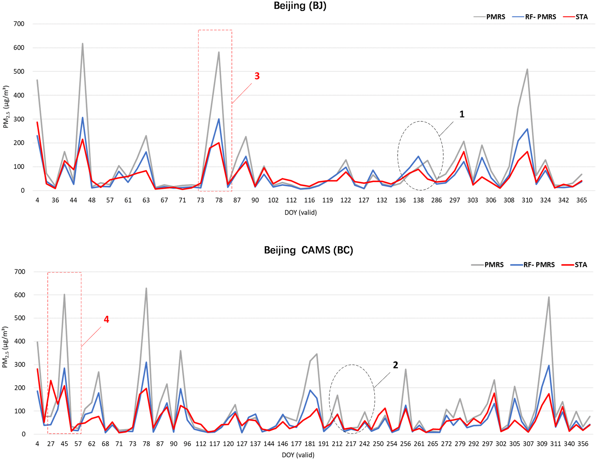
Figure 4Three PM2.5 time series at the Beijing (BJ) and Beijing-CAMS (BC) sites under their respective DOYs in 2017. Here, DOY (valid) means the day of the year with valid AOD, FMF, and other PM2.5-related data. Gray, blue, and red lines represent PM2.5 values of PMRS, RF-PMRS, and the stations (STA), respectively. The red boxes and black circles select a specific period for analysis.
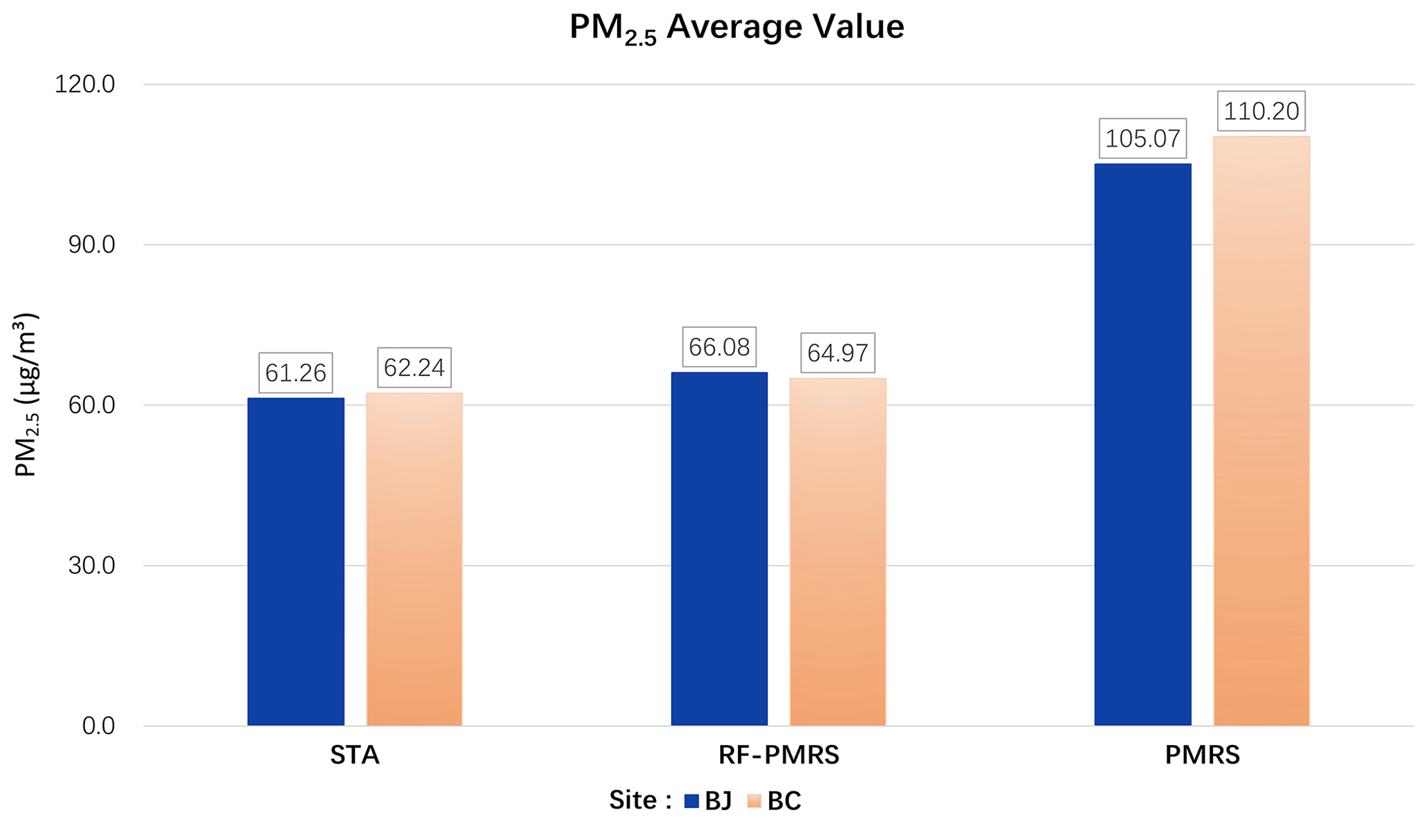
Figure 5Annual average PM2.5 values from the stations (left), RF-PMRS (middle), and PMRS (right) at the BJ and BC sites.
To visually compare the optimization effect, Fig. 6 plots the PM2.5 bias distribution patterns for two methods. From the boxplot, the average PM2.5 bias of RF-PMRS is close to zero (less than 5 µg m−3), which is greatly lower than that of PMRS. Moreover, PMRS PM2.5 has a larger deviation range, which manifests in two aspects. One is the maximum bias; specifically, it has exceeded 100 µg m−3 at the BC site. The other is the overall distribution of the data bias; the BJ site ones are mostly distributed below 0, indicating an obvious overestimation. As for RF-PMRS, the above circumstances are not obviously reflected in it. In addition, as can be seen from the indicators, the RMSE and MAE of RF-PMRS PM2.5 decrease by about half in comparison with PMRS. The experiment has confirmed that the RF-PMRS PM2.5 values have a strong linear relationship with the ground truth at both sites, with R around 0.8 (0.82 at BJ and 0.78 at BC). Such a large optimization effect is attributed to the VEf expression replacement to the fitted RF model.
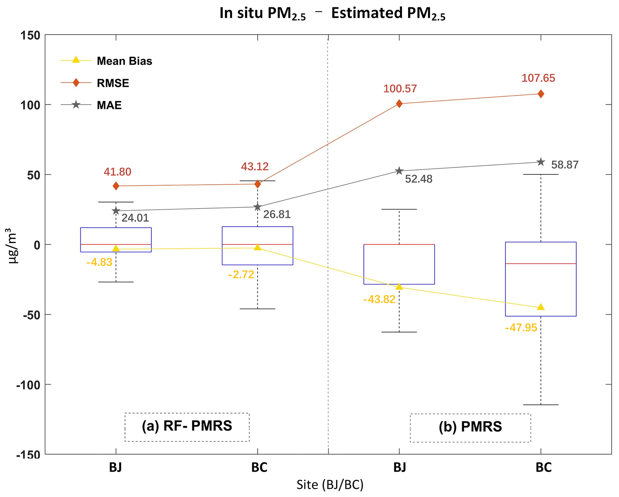
Figure 6Boxplots of (a) RF-PMRS and (b) PMRS PM2.5 bias at the BJ and BC sites. The upper (lower) black line of each box represents the largest (smallest) value, the upper (lower) blue border represents the upper (lower) quartile, and the red line denotes the median. The yellow, orange, and gray symbols are the MB, RMSE, and MAE of the corresponding PM2.5 concentration.
4.3 Generalization performance of RF-PMRS
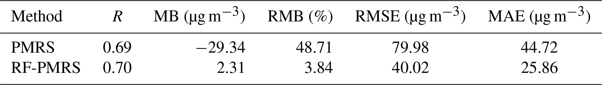
Then, we estimate PM2.5 based on PMRS and RF-PMRS within North China in 2017 (Fig. 1 exhibits the distribution pattern of the validation stations). Table 4 shows the accuracy statistics. It can be seen that RF-PMRS greatly reduces the bias (about 44.87 %), with an MB of about 2.31 µg m−3. Similar to the results at the sites, the RF-PMRS method can derive PM2.5 concentration with practically no overestimation (underestimation). Although there is not much difference in the R values of the two models (R of RF-PMRS is only improved by 0.01), RMSE and MAE decrease by about 39.96 and 18.86 µg m−3, respectively. As a result, the optimized method deserves to be considered excellent.
Table 4Validation results of PMRS and RF-PMRS PM2.5 in North China.
Meanwhile, the PM2.5 scatterplots are presented below. As depicted in Fig. 7, there are sufficient estimated samples (28 305) in the NC region, which guarantees the credibility of our validation results. In general, the RF-PMRS PM2.5 values are distributed around the 1:1 reference line evenly, with a slightly higher R of 0.70 compared to that of the original method. The slope of the linear fitting relationship reaches 0.82, which indicates that the proposed method greatly reduces the overestimation of PMRS with a linear slope of 1.46. Although the overall performance of the RF-PMRS estimations maintains an excellent level, defects do remain. To be specific, in areas with high PM2.5 concentration (especially greater than 150 µg m−3), RF-PMRS results exist with a slight underestimation. It may be caused by the relatively small number of high-value PM2.5 points (only 1319 out of 28 305), which makes it difficult to adequately reflect the fitting effect of the method.
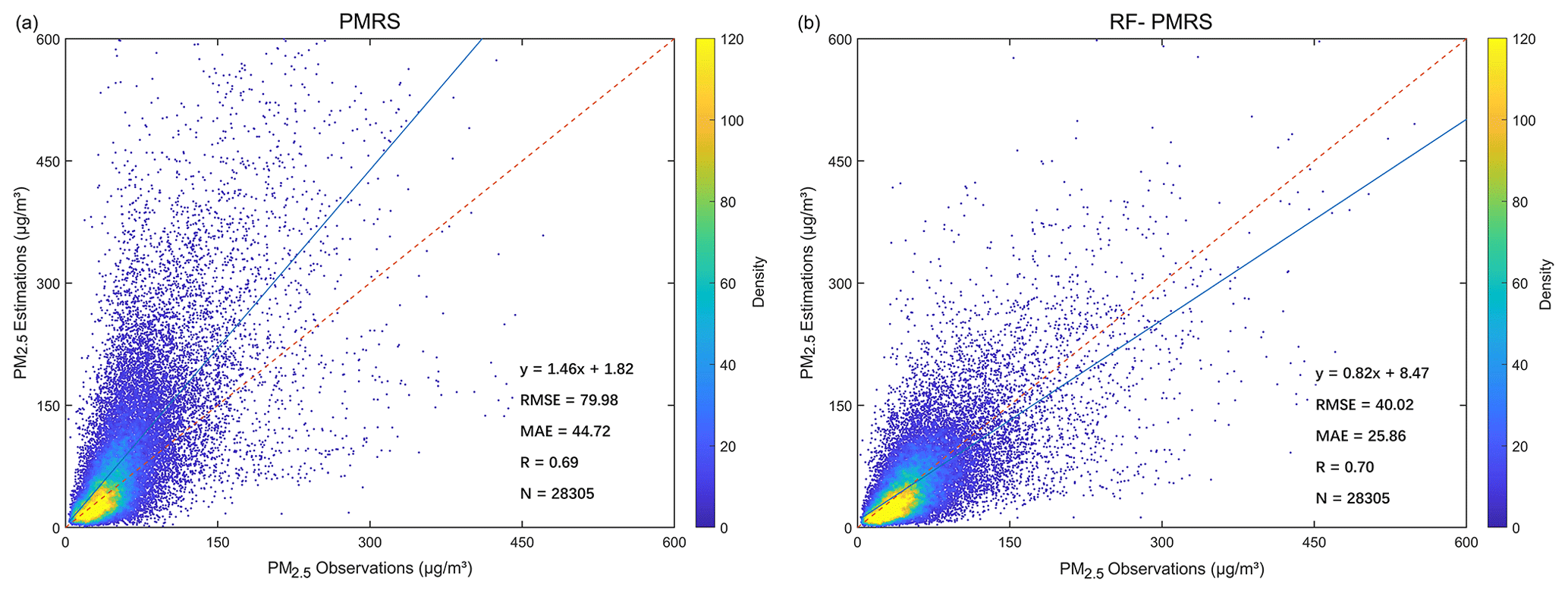
Figure 7Validation scatterplots of PM2.5 results from (a) PMRS and (b) RF-PMRS. Dashed red lines are 1:1 reference lines, and solid blue lines stand for the linear fits. The right legends show the point densities (frequency) represented by different colors.
As for RF-PMRS, the deviation is reduced to a large extent, so the maps of the probability density function based on the bias of PMRS and RF-PMRS are further drawn. Figure 8 visualizes the probability densities within different bias ranges. In terms of distribution characteristics, the overall bias of RF-PMRS from the value of 0 (solid black line) is small. About the curve shape, it is high and narrow, manifesting in the fact that the bias has a lower standard deviation (SD) and is more prone to appear around the mean. However, PMRS shows a more discrete distribution pattern, and there are many outliers outside the range of greater than 600 µg m−3. Simultaneously, as can be concluded from the three boxes, within the bias range of ±20 and ±40 µg m−3, the data numbers of RF-PMRS results increase by 8.32 % and 12.81 %, respectively. Outside the range of ±100 µg m−3, the number decreases by 9.10 %. Therefore, as far as the accuracy is concerned, RF-PMRS results have lower bias and better stability.
In addition to the above general performance comparison in Sect. 4.3, Fig. 9 presents the annual average RMSE spatial distribution of PMRS and RF-PMRS PM2.5 at NC stations. The two methods show a large deviation in the middle and southeast, and the RMSE map of PMRS has more red points. However, RF-PMRS can weaken this phenomenon very well since its RMSE representative colors are generally light. In particular, the proportion of dark-red sites (RMSE greater than 60 µg m−3) decreases from 65.44 % (PMRS) to 4.15 % (RF-PMRS). In the areas where the ground stations are clustered, the deviation also reduces significantly.
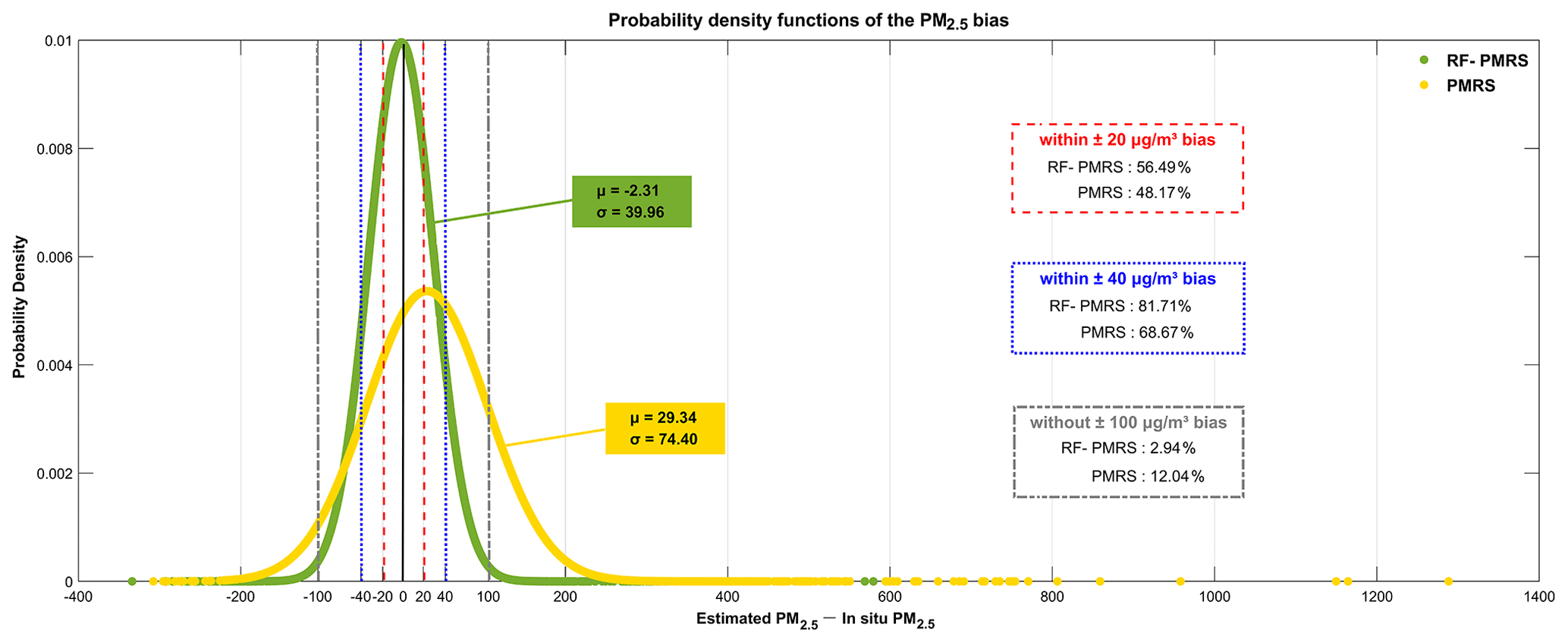
Figure 8Probability density functions of PMRS (yellow) and RF-PMRS (green) PM2.5 bias. The dotted red, blue, and gray lines indicate the bias boundaries of ±20, ±40, and ±100 µg m−3, respectively. µ and σ represent the mean value and standard deviation of each data point.
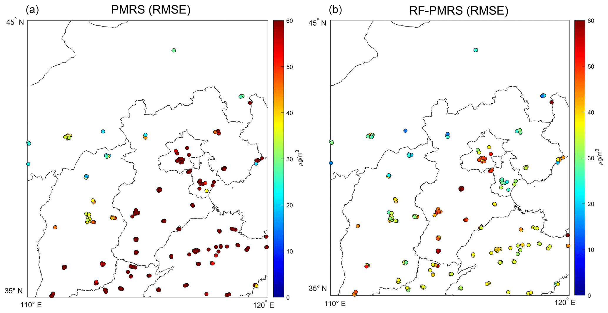
Figure 9RMSE of the yearly average PM2.5 concentration values between different models and ground stations (a PMRS PM2.5, b RF-PMRS PM2.5). Note that the top red color of the RMSE legend indicates RMSE values equal to or greater than 60 µg m−3.
In a word, the above analysis demonstrates that compared with the simple quadratic polynomial relationship (Eq. 9), the established RF model in RF-PMRS can more accurately capture the relationship between VEf and multiple variables, thereby improving the PM2.5 estimation accuracy.
5.1 Accuracy comparison of PMRS using MODIS FMF and Phy-DL FMF
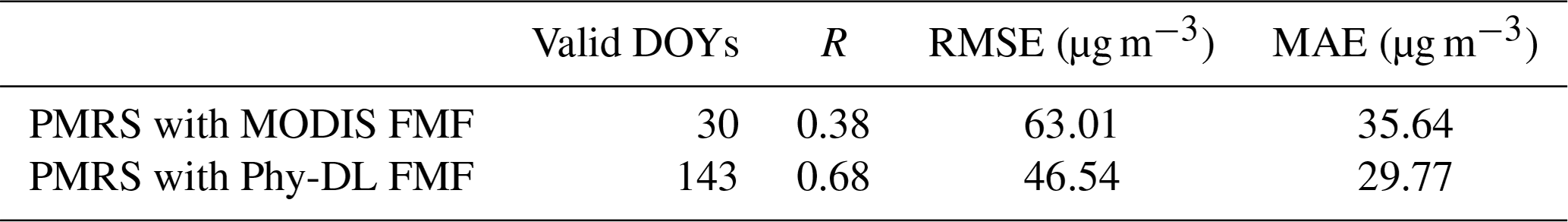
To confirm the superiority of the Phy-DL FMF data adopted in our method framework, the experiment takes the BJ and BC sites as examples (in 2017) and then compares the PM2.5 accuracy and the number of effective days calculated by PMRS based on different FMF values. Table 5 presents the overall day-level results. Here, “DOY” means the day of the year and “valid” means that all variables related to the PM2.5 calculation are valid. As can be seen, after the FMF replacement, the number of valid DOYs grows (an increase of 113 d), which illustrates that the number of effective PM2.5 concentrations has gone up by about 5 times. Moreover, the accuracy has been significantly enhanced, with R having increased by about 0.30 and RMSE and MAE having decreased by 26.14 % and 16.47 %, accordingly. On the whole, Phy-DL FMF contributes to the improvement in PMRS results, signifying the first step in optimization of the proposed RF-PMRS method is effective.
Table 5Validation results of the PMRS method using different FMF data. The valid DOY refers to the number of days for which the AOD, FMF, and other data are not missing when calculating PM2.5. Note that since the valid days of the two schemes are different, the MB and RMB are not compared.
5.2 Performance compared with other ML models
Different machine learning models are suitable for diverse research data, and decision tree (DT) models can better fit experiments with fewer variables, such as this study. For comparison, except for RF, the extremely randomized tree (ERT) (Geurts et al., 2006) and gradient boosting decision tree (GBDT) (Friedman, 2001) models have also been established. The results of training VEf based on the above three DT models are presented in Tables 6 and 7. By contrast, RF performs best in CV and IV experiments, as indicated by the multiple accuracy indicators. Although the ERT and GBDT models are comparable to RF in some indicators, there exists a certain degree of overfitting in the above two models, which is manifested in the fact that their IV results are clearly worse than their respective CV ones. Thus, the RF model is applied to our study.
Table 6Cross-validation results for comparison of the decision tree models for training VEf. N represents the number of data, and VEf has no unit.
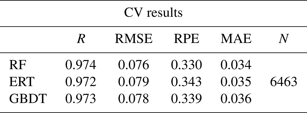
Table 7Isolated-validation results in comparison of the decision tree models for training VEf. The indicators are the same as those in Table 6.
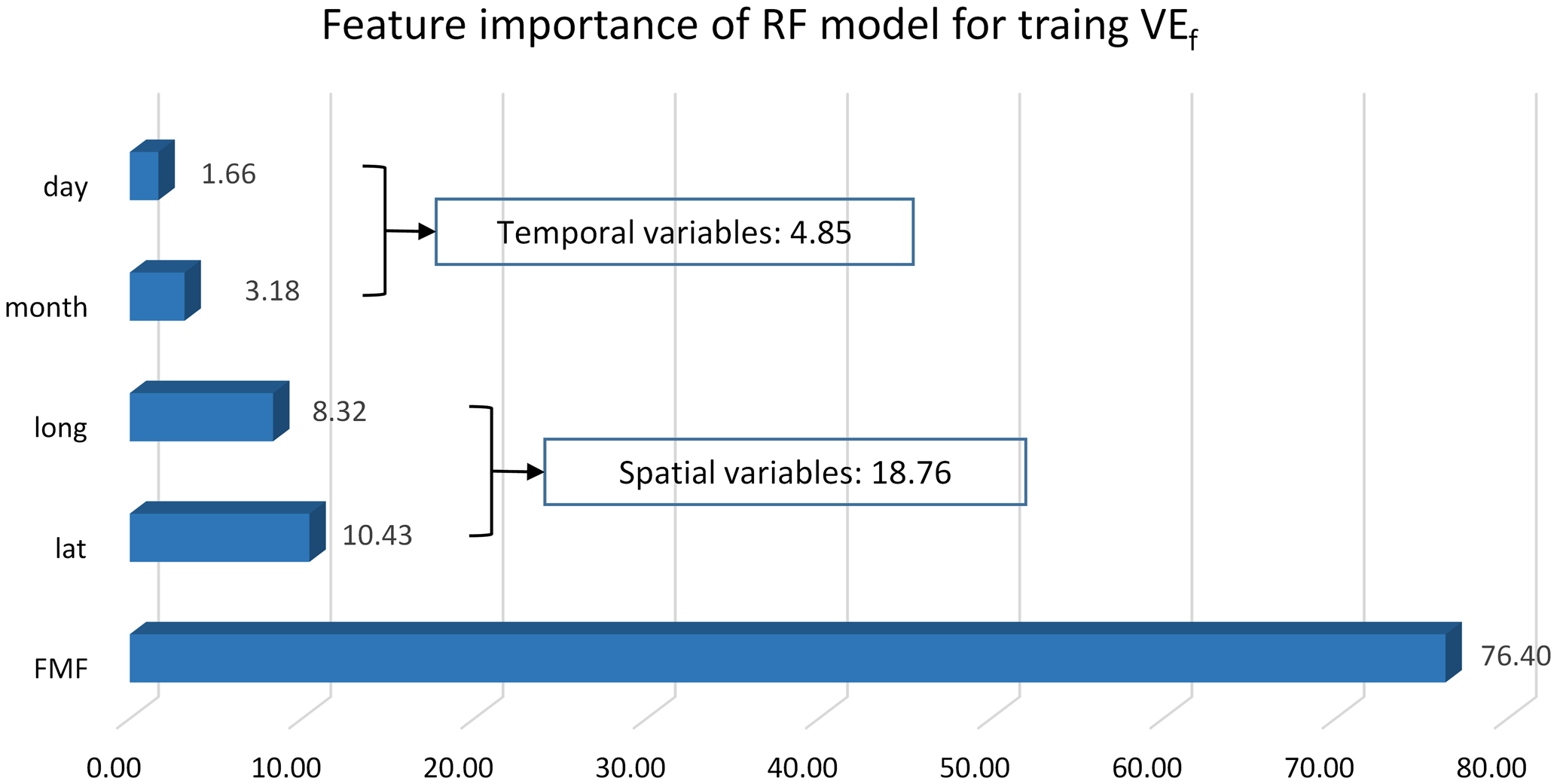
5.3 Feature importance of the embedded RF model
Additionally, the feature importance of RF is calculated to evaluate the contribution of model predictors to VEf simulation. Figure B2 (in Appendix B) shows the results by normalization (taking 100 as the total). Without a doubt, FMF accounts for the largest proportion, about 76.4 %, which is consistent with the analysis when selecting the VEf-related variables (see Sect. 3.2). The contribution of spatiotemporal variables is about of FMF, which indirectly affirms the credibility of RF feature learning. Also, it provides a basis for further uncertainty optimization of VEf and PM2.5 accuracy.
5.4 Advantages and disadvantages
5.4.1 Advantages of the RF-PMRS method
From the perspective of model parameter optimization, this paper embeds RF to replace the subprocess parameter of the semi-empirical physical model. As a result, the proposed method, RF-PMRS, reduces the uncertainty in the complex physical parameter (i.e., VEf) based on the estimation steps of strong physical significance and realizes the coupling of machine learning and the model mechanism. The proposed method does not rely on the PM2.5 values of ground stations and is not affected by the station density and distribution mode, which can estimate the PM2.5 concentration independently.
Meanwhile, as for the method, we construct the VEf model based on RF using high-precision point data and extend it to surface data for PM2.5 estimations. The experimental results demonstrate the overall performance of the model (Sect. 4.1) and its applicability in North China (Sect. 4.2 to 4.3), showing that the method has certain universality from the point scale to the surface scale.
-
The overall performance of the model is high. We use the ground data of nine AERONET sites around the world to train the RF model and simulate the VEf values; the site distribution is relatively uniform, and the number of training data is sufficient. Table 1 shows a total of 6463 data matching pairs in the training period, which is enough to establish a credible RF model. Table 3 results show that in IV experiments, the accuracy of the model is good and can be generalized in different periods. For VEf, the model shows both high internal accuracy (CV) and external accuracy (IV), so it can be generalized in regions with different aerosol types.
-
In the subsequent PM2.5 estimation, the model displays high applicability in North China. From the perspective of model construction, the four aerosol types are the classification basis of the training data, and comprehensive modeling can improve the generalization performance. Also, the addition of spatiotemporal variables can increase the model applicability in North China. On the other hand, the number of stations used in an area does not determine the regional accuracy of the established model, which can be derived from our results. Compared with the PM2.5 ground measurements in the NC region, the relative deviation of the RF-PMRS PM2.5 is only 2.31 µg m−3, which confirms that RF can represent the relationships within North China.
5.4.2 Limitations on the scope of the validation region
However, there are still some shortcomings, mainly manifested in the scope of the validation region. Due to limited experimental data, we only conduct experiments in North China (the main aerosol type is urban–industrial). The main reasons are as follows.
-
Insufficient ρf,dry value.
As the empirical value in the semi-physical empirical model, the ρf,dry value is often obtained by field measurements and induction. The insufficient ρf,dry values hinder the derivation of PM2.5 in other regions, and more research results are needed.
-
Disclosure limits on global PM2.5 ground measurements.
Accurate and sufficient in situ PM2.5 values allow for the verification of estimated PM2.5 results.
-
Fewer public AERONET sites.
Therefore, only the BJ and BC sites in North China are used for representative point-scale validation.
5.4.3 Data differences and uncertainty analysis
In the RF-PMRS method, the VEf model constructed by high-precision site data is generalized to surface data for validation, and the data types involved are as follows.
-
AERONET AOD vs. MODIS AOD.
Two types of AOD are used for different experimental steps, among which AERONET AOD is applied to calculate the true values of VEf for establishing the RF simulation model. The RF model construction is a step of PM2.5 estimation (as the VEf variable in Eq. 7). MODIS AOD is satellite AOD data, the most commonly used remote sensing data for large-scale retrieval of PM2.5. It is an important variable for PM2.5 estimation in RF-PMRS (as the AOD variable in Eq. 7). Thus, there is no error in the PM2.5 calculation caused by AOD category replacement.
As for uncertainty, AERONET AOD provides truth values for calculating VEf, which theoretically has negligible uncertainty, and the simulation accuracy of VEf represents its influence on estimating PM2.5 to a certain extent. It is generally considered that MODIS AOD has guaranteed quality and sufficient accuracy to be used directly.
-
S-FMF vs. Phy-DL FMF.
S-FMF is obtained directly from the AERONET monitoring sites and is one of the variables of the RF model (as the FMF variable in Eq. 10). In the point-to-surface extension, Phy-DL FMF is introduced into the RF model to replace S-FMF, and the 2017 VEf values are obtained. The basis of the above replacement is that the accuracy of Phy-DL FMF is relatively consistent with that of S-FMF (Yan et al., 2022). Moreover, Phy-DL FMF data are applied to the PM2.5 estimation steps (as the FMF variable in Eq. 7) for a wider range of validation experiments. The results show that the PM2.5 concentration estimated by RF-PMRS has high accuracy, proving the credibility of Phy-DL FMF.
-
FMF uncertainty.
Different surface data sources may affect the PM2.5 results, introducing some uncertainty. Section 5.1 compares the PM2.5 accuracy using two FMF data in 2017. The data missing time for MODIS FMF and Phy-DL FMF in North China are different, which can be found in the statistics on their respective available days (referred to as valid DOYs). There are far more valid days based on Phy-DL FMF than MODIS FMF (143 and 31 d), demonstrating the superiority of Phy-DL FMF. Although the specific validation time of two FMF varies, the overall accuracy of the PM2.5 estimation (which can be regarded as the average accuracy over the year) shows that the Phy-DL FMF increases R to 0.68 (MODIS FMF: 0.38) with low uncertainty.
-
ρf,dry uncertainty.
As introduced earlier, the ρf,dry value is often obtained by field measurements. In our study, we select 1.5 g cm−3 as the ρf,dry value for North China. There are certain variations in the empirical values of different regions, and there will be errors (uncertainty) between the values in Beijing and other places in the NC region. However, our experimental area is not large, and we use 1.5 g cm−3 to represent ρf,dry of the whole region, which has been applied in previous articles (Zhang and Li, 2015; Li et al., 2016).
-
Uncertainty between variable resolutions.
In most experiments, the lowest resolution of all data will be taken as the unified resolution when obtaining data values. The different data may lose some spatial details during the upsampling–downsampling process, which brings uncertainty to the estimation results. In the RF-PMRS method, there is no such uncertainty problem. We set 1∘ as the unified spatial unit and take the longitude and latitude of each cell's center as the reference longitude and latitude. The variables in the Data section are spatially matched to ground sites at their respective resolutions, and the space–time matching method has been described in the Methods section. So, all kinds of data uncertainties only exist in their instrument measurement or statistical release.
Overall, RF-PMRS shows excellent estimation performance in North China, and the accuracy of surface PM2.5 estimation based on remote sensing data is guaranteed. Next, with the improvement in related experimental data, we will verify our proposed method in a broader range and continuously optimize it from all aspects.
Among various satellite remote sensing methods for PM2.5 retrieval, the semi-empirical physical approach has strong physical significance and clear calculation steps and derives the PM2.5 mass concentration independently of in situ observations. However, the parameters of optical properties are difficult to express, requiring them to be optimized. Hence, the study proposes a method (RF-PMRS) that embeds machine learning in a physical model to obtain surface PM2.5: (1) based on the PMRS method, select the Phy-DL FMF product with a combined mechanism, and (2) use the RF model to fit the parameter VEf, rather than a simple quadratic polynomial. In the point-to-surface validation, RF-PMRS shows great optimized performance. Experiments at two AERONET sites show that R reaches up to 0.8. In North China, RMSE decreases by 39.95 µg m−3 with a 44.87 % reduction in relative deviation. In the future, we will further explore the combination of an atmospheric mechanism and machine learning and then research the PM2.5 retrieval methods with physical meaning and higher accuracy.
A1 The 10-fold cross-validation and isolated validation
The sample-based 10-fold cross-validation method is applied to tune the model parameters and test the internal accuracy of our model. The original dataset is randomly divided into 10 parts, 9 of which are used as the training set for model fitting, with the remaining 1 used for prediction; then the cross-validation process is repeated for 10 rounds until each data point has been used as the test set.
At the same time, when verifying the RF-based VEf model, the dataset in the period that did not participate in the training in Table 1 is used for isolated validation.
A2 Statistical indicators
where m is the total number of observations; i is the number of measurements; yi is the ith observation; fi is the corresponding estimation result; and and are the averages of all observations and estimates, respectively.
A3 Parameter adjustments of the RF model
The four parameters of RF are adjusted; i.e., the correlation coefficient r changes with the (a) number of trees, (b) maximum depth, (c) maximum number of features when splitting, and (d) minimum number of split samples. Experiments show that the maximum depth varies greatly in a small range. To prevent overfitting, the four parameters of RF are adjusted to 60, 10, 2, and 8. It can ensure high accuracy while improving training efficiency.

Figure B1The time series of PMRS and RF-PMRS PM2.5 bias at the Beijing and Beijing-CAMS sites under their respective DOYs in 2017. The orange line represents the bias between the PM2.5 values of PMRS and the stations, while the blue one indicates the PM2.5 difference between RF-PMRS and the stations.
All relevant codes as well as the intermediate data of this work are archived at https://doi.org/10.5281/zenodo.7183822 (Jin, 2022). The MCD19A2 data can be downloaded at https://doi.org/10.5067/MODIS/MCD19A2.006 (Lyapustin and Wang, 2015). Detailed information about the Phy-DL FMF dataset can be found at https://doi.org/10.5281/zenodo.5105617 (Yan, 2021). Meteorological data used in this work were obtained from https://doi.org/10.24381/cds.adbb2d47 (Hersbach et al., 2018). AERONET data were downloaded from https://aeronet.gsfc.nasa.gov/ (Giles et al., 2019).
CJ: data curation, methodology, formal analysis, writing (original draft). QY: conceptualization, supervision, project administration, writing (review and editing). TL: resources, methodology, writing (review and editing), formal analysis. YW: methodology, validation, writing (review and editing). LZ: supervision, writing (review and editing).
The contact author has declared that none of the authors has any competing interests.
Publisher’s note: Copernicus Publications remains neutral with regard to jurisdictional claims in published maps and institutional affiliations.
We gratefully acknowledge the Level-1 and Atmosphere Archive & Distribution System (LAADS), the ECMWF, the AERONET project, and the CNEMC for, respectively, providing the MODIS products, the meteorological data, the ground aerosol data, and the surface PM2.5 concentration. We also thank other institutions which provide related data in this work.
This research has been supported by the National Key R&D Program of China (grant no. 2022YFB3903403), the Fundamental Research Funds for the Central Universities (grant nos. 2042023kfyq04 and 2042023kf1007), the National Natural Science Foundation of China (grant nos. 42201359), and the Guangdong Basic and Applied Basic Research Foundation (grant no. 2022A1515010492).
This paper was edited by Po-Lun Ma and reviewed by three anonymous referees.
Belgiu, M. and Drăguţ, L.: Random forest in remote sensing: A review of applications and future directions, ISPRS J. Photogramm., 114, 24–31, https://doi.org/10.1016/j.isprsjprs.2016.01.011, 2016.
Bowe, B., Xie, Y., Li, T., Yan, Y., Xian, H., and Al-Aly, Z.: The 2016 global and national burden of diabetes mellitus attributable to PM2.5 air pollution, Lancet Planet. Health, 2, e301–e312, https://doi.org/10.1016/S2542-5196(18)30140-2, 2018.
Chen, X., de Leeuw, G., Arola, A., Liu, S., Liu, Y., Li, Z., and Zhang, K.: Joint retrieval of the aerosol fine mode fraction and optical depth using MODIS spectral reflectance over northern and eastern China: Artificial neural network method, Remote Sens. Environ., 249, 112006, https://doi.org/10.1016/j.rse.2020.112006, 2020.
Friedman, J. H.: Greedy function approximation: a gradient boosting machine, Ann. Stat., 29, 1189–1232, 2001.
Gao, J., Zhou, Y., Wang, J., Wang, T., and Wang, W. X.: Inter-comparison of WPSTM-TEOMTM-MOUDITM and investigation on particle density, Huan Jing Ke Xue, 28, 1929–1934, https://doi.org/10.3321/j.issn:0250-3301.2007.09.005, 2007.
Gao, L., Li, J., Chen, L., Zhang, L., and Heidinger, A. K.: Retrieval and validation of atmospheric aerosol optical depth from AVHRR over China, IEEE T. Geosci. Remote, 54, 6280–6291, https://doi.org/10.1109/TGRS.2016.2574756, 2016.
Geng, G., Zhang, Q., Martin, R. V., van Donkelaar, A., Huo, H., Che, H., Lin, J., and He, K.: Estimating long-term PM2.5 concentrations in China using satellite-based aerosol optical depth and a chemical transport model, Remote Sens. Environ., 166, 262–270, https://doi.org/10.1016/j.rse.2015.05.016, 2015.
Geurts, P., Ernst, D., and Wehenkel, L.: Extremely randomized trees, Mach. Learn., 63, 3–42, https://doi.org/10.1007/s10994-006-6226-1, 2006.
Giles, D. M., Holben, B. N., Eck, T. F., Smirnov, A., Sinyuk, A., Schafer, J., Sorokin, M. G., and Slutsker, I.: Aerosol robotic network (AERONET) version 3 aerosol optical depth and inversion products, in: American Geophysical Union (AGU) 98th Fall Meeting Abstracts, New Orleans, America, 11–15 December 2017, A11O-01, 2017AGUFM.A11O..01G, 2017.
Giles, D. M., Sinyuk, A., Sorokin, M. G., Schafer, J. S., Smirnov, A., Slutsker, I., Eck, T. F., Holben, B. N., Lewis, J. R., Campbell, J. R., Welton, E. J., Korkin, S. V., and Lyapustin, A. I.: Advancements in the Aerosol Robotic Network (AERONET) Version 3 database – automated near-real-time quality control algorithm with improved cloud screening for Sun photometer aerosol optical depth (AOD) measurements, Atmos. Meas. Tech., 12, 169–209, https://doi.org/10.5194/amt-12-169-2019, 2019 (data available at: https://aeronet.gsfc.nasa.gov/, last access: 30 September 2022).
Gupta, P. and Christopher, S. A.: Particulate matter air quality assessment using integrated surface, satellite, and meteorological products: Multiple regression approach, J. Geophys. Res.-Atmos., 114, D14205, https://doi.org/10.1029/2008JD011496, 2009.
Hand, J. L. and Kreidenweis, S. M.: A new method for retrieving particle refractive index and effective density from aerosol size distribution data, Aerosol Sci. Technol., 36, 1012–1026, https://doi.org/10.1080/02786820290092276, 2002.
Hänel, G. and Thudium, J.: Mean bulk densities of samples of dry atmospheric aerosol particles: A summary of measured data, Pure Appl. Geophys., 115, 799–803, https://doi.org/10.1007/BF00881211, 1977.
He, J., Yuan, Q., Li, J., and Zhang, L.: PoNet: A universal physical optimization-based spectral super-resolution network for arbitrary multispectral images, Inform. Fusion, 80, 205–225, https://doi.org/10.1016/j.inffus.2021.10.016, 2022.
He, J., Li, J., Yuan, Q., Shen, H., and Zhang, L.: Spectral Response Function-Guided Deep Optimization-Driven Network for Spectral Super-Resolution, IEEE T. Neur. Net. Lear., 99, 1–15, https://doi.org/10.1109/TNNLS.2021.3056181, 2021.
Ho, T.: Random decision forests, in: Proceedings of 3rd International Conference on Document Analysis and Recognition, Montreal, QC, Canada, 14–16 August 1995, 278–282, https://doi.org/10.1109/ICDAR.1995.598994, 1995.
Hersbach, H., Bell, B., Berrisford, P., Biavati, G., Horányi, A., Muñoz Sabater, J., Nicolas, J., Peubey, C., Radu, R., Rozum, I., Schepers, D., Simmons, A., Soci, C., Dee, D., and Thépaut, J.-N.: ERA5 hourly data on single levels from 1979 to present, Copernicus Climate Change Service (C3S) Climate Data Store (CDS) [data set], https://doi.org/10.24381/cds.adbb2d47, 2018.
Holben, B. N., Eck, T. F., Slutsker, I., Tanré, D., Buis, J. P., Setzer, A., Vermote, E., Reagan, J. A., Kaufman, Y. J., Nakajima, T., Lavenu, F., Jankowiak, I., and Smirnov, A.: AERONET–A federated instrument network and data archive for aerosol characterization, Remote Sens. Environ., 66, 1–16, https://doi.org/10.1016/S0034-4257(98)00031-5, 1998.
Irrgang, C., Boers, N., Sonnewald, M., Barnes, E. A., Kadow, C., Staneva, J., and Saynisch-Wagner, J.: Towards neural Earth system modelling by integrating artificial intelligence in Earth system science, Nat. Mach. Intell., 3, 667–674, https://doi.org/10.1038/s42256-021-00374-3, 2021.
Jin, C.: An optimized semi-empirical physical approach for satellite-based PM2.5 retrieval: using random forest model to simulate the complex parameter, Zenodo [code], https://doi.org/10.5281/zenodo.7183822, 2022.
Koelemeijer, R. B. A., Homan, C. D., and Matthijsen, J.: Comparison of spatial and temporal variations of aerosol optical thickness and particulate matter over Europe, Atmos. Environ., 40, 5304–5315, https://doi.org/10.1016/j.atmosenv.2006.04.044, 2006.
Kokhanovsky, A. A., Prikhach, A. S., Katsev, I. L., and Zege, E. P.: Determination of particulate matter vertical columns using satellite observations, Atmos. Meas. Tech., 2, 327–335, https://doi.org/10.5194/amt-2-327-2009, 2009.
Lee, J.-B., Lee, J.-B., Koo, Y.-S., Kwon, H.-Y., Choi, M.-H., Park, H.-J., and Lee, D.-G.: Development of a deep neural network for predicting 6 h average PM2.5 concentrations up to 2 subsequent days using various training data, Geosci. Model Dev., 15, 3797–3813, https://doi.org/10.5194/gmd-15-3797-2022, 2022.
Li, T., Shen, H., Zeng, C., Yuan, Q., and Zhang, L.: Point-surface fusion of station measurements and satellite observations for mapping PM2.5 distribution in China: Methods and assessment, Atmos. Environ., 152, 477–489, https://doi.org/10.1016/j.atmosenv.2017.01.004, 2017.
Li, Z., Zhang, Y., Shao, J., Li, B., Hong, J., Liu, D., Li, D., Wei, P., Li, W., Li, L., Zhang, F., Guo, J., Deng, Q., Wang, B., Cui, C., Zhang, W., Wang, Z., Lv, Y., Xu, H., Chen, X., Li, L., and Qie, L.: Remote sensing of atmospheric particulate mass of dry PM2.5 near the ground: Method validation using ground-based measurements, Remote Sens. Environ., 173, 59–68, https://doi.org/10.1016/j.rse.2015.11.019, 2016.
Lyapustin, A., Wang, Y., Laszlo, I., Kahn, R., Korkin, S., Remer, L., Levy, R., and Reid, J. S.: Multiangle implementation of atmospheric correction (MAIAC): 2. Aerosol algorithm, J. Geophys. Res.-Atmos., 116, D03211, https://doi.org/10.1029/2010JD014986, 2011.
Lyapustin, A., Wang, Y., Xiong, X., Meister, G., Platnick, S., Levy, R., Franz, B., Korkin, S., Hilker, T., Tucker, J., Hall, F., Sellers, P., Wu, A., and Angal, A.: Scientific impact of MODIS C5 calibration degradation and C6+ improvements, Atmos. Meas. Tech., 7, 4353–4365, https://doi.org/10.5194/amt-7-4353-2014, 2014.
Lyapustin, A. and Wang, Y.: MCD19A2 MODIS/Terra+Aqua Aerosol Optical Thickness Daily L2G Global 1km SIN Grid, NASA LP DAAC [data set], https://doi.org/10.5067/MODIS/MCD19A2.006, 2015.
Lyu, B., Huang, R., Wang, X., Wang, W., and Hu, Y.: Deep-learning spatial principles from deterministic chemical transport models for chemical reanalysis: an application in China for PM2.5, Geosci. Model Dev., 15, 1583–1594, https://doi.org/10.5194/gmd-15-1583-2022, 2022.
Ma, Z., Hu, X., Huang, L., Bi, J., and Liu, Y.: Estimating ground-Level PM2.5 in China using satellite remote sensing, Environ. Sci. Technol., 48, 7436–7444, https://doi.org/10.1021/es5009399, 2014.
Pope III, C. A., Burnett, R. T., Thun, M. J., Calle, E. E., Krewski, D., Ito, K., and Thurston, G. D.: Lung cancer, cardiopulmonary mortality, and long-term exposure to fine particulate air pollution, JAMA, 287, 1132–1141, https://doi.org/10.1001/jama.287.9.1132, 2002.
Raut, J.-C. and Chazette, P.: Assessment of vertically-resolved PM10 from mobile lidar observations, Atmos. Chem. Phys., 9, 8617–8638, https://doi.org/10.5194/acp-9-8617-2009, 2009.
Rodriguez, J. D., Perez, A., and Lozano, J. A.: Sensitivity analysis of k-fold cross validation in prediction error estimation, IEEE T. Pattern Anal., 32, 569–575, https://doi.org/10.1109/TPAMI.2009.187, 2009.
Shi, X., Zhao, C., Jiang, J. H., Wang, C., Yang, X., and Yung, Y. L.: Spatial representativeness of PM2.5 concentrations obtained using observations from network stations, J. Geophys. Res.-Atmos., 123, 3145–3158, https://doi.org/10.1002/2017JD027913, 2018.
Simmons, A. J., Untch, A., Jakob, C., Kållberg, P., and Undén, P.: Stratospheric water vapour and tropical tropopause temperatures in ECMWF analyses and multi-year simulations, Q. J. Roy. Meteor. Soc., 125, 353–386, https://doi.org/10.1002/qj.49712555318, 1999.
Van Donkelaar, A., Martin, R. V., and Park, R. J.: Estimating ground-level PM2.5 using aerosol optical depth determined from satellite remote sensing, J. Geophys. Res.-Atmos., 111, D21201, https://doi.org/10.1029/2005JD006996, 2006.
Wang, Y., Yuan, Q., Li, T., Shen, H., Zheng, L., and Zhang, L.: Evaluation and comparison of MODIS Collection 6.1 aerosol optical depth against AERONET over regions in China with multifarious underlying surfaces, Atmos. Environ., 200, 280–301, https://doi.org/10.1016/j.atmosenv.2018.12.023, 2019.
Wu, X., Wang, Y., He, S., and Wu, Z.: ratio prediction based on a long short-term memory neural network in Wuhan, China, Geosci. Model Dev., 13, 1499–1511, https://doi.org/10.5194/gmd-13-1499-2020, 2020.
Xiao, Y., Wang, Y., Yuan, Q., He, J., and Zhang, L.: Generating a long-term (2003–2020) hourly 0.25∘ global PM2.5 dataset via spatiotemporal downscaling of CAMS with deep learning (DeepCAMS), Sci. Total Environ., 848, 157747, https://doi.org/10.1016/j.scitotenv.2022.157747, 2022.
Xu, P., Chen, Y., and Ye, X.: Haze, air pollution, and health in China, Lancet, 382, 2067, https://doi.org/10.1016/S0140-6736(13)62693-8, 2013.
Yan, X., Zang, Z., Li, Z., Luo, N., Zuo, C., Jiang, Y., Li, D., Guo, Y., Zhao, W., Shi, W., and Cribb, M.: A global land aerosol fine-mode fraction dataset (2001–2020) retrieved from MODIS using hybrid physical and deep learning approaches, Earth Syst. Sci. Data, 14, 1193–1213, https://doi.org/10.5194/essd-14-1193-2022, 2022.
Yan, X., Li, Z., Shi, W., Luo, N., Wu, T., and Zhao, W.: An improved algorithm for retrieving the fine-mode fraction of aerosol optical thickness, part 1: Algorithm development, Remote Sens. Environ., 192, 87–97, https://doi.org/10.1016/j.rse.2017.02.005, 2017.
Yan, X.: Physical and deep learning retrieved fine mode fraction (Phy-DL FMF), Zenodo [data set], https://doi.org/10.5281/zenodo.5105617, 2021.
Yang, Q., Yuan, Q., Li, T., and Yue, L.: Mapping PM2.5 concentration at high resolution using a cascade random forest based downscaling model: Evaluation and application, J. Clean. Prod., 277, 123887, https://doi.org/10.1016/j.jclepro.2020.123887, 2020.
Yuan, Q., Shen, H., Li, T., Li, Z., Li, S., Jiang, Y., Xu, H., Tan, W., Yang, Q., Wang, J., Gao, J., and Zhang, L.: Deep learning in environmental remote sensing: Achievements and challenges, Remote Sens. Environ., 241, 111716, https://doi.org/10.1016/j.rse.2020.111716, 2020.
Zhang, Y., Li, Z., Bai, K., Wei, Y., Xie, Y., Zhang, Y., Ou, Y., Cohen, J., Zhang, Y., Peng, Z., Zhang, X., Chen, C., Hong, J., Xu, H., Guang, J., Lv, Y., Li, K., and Li, D.: Satellite remote sensing of atmospheric particulate matter mass concentration: Advances, challenges, and perspectives, Fundamental Research, 1, 240–258, https://doi.org/10.1016/j.fmre.2021.04.007, 2021.
Zhang, Y., Li, Z., Chang, W., Zhang, Y., de Leeuw, G., and Schauer, J. J.: Satellite observations of PM2.5 changes and driving factors based forecasting over China 2000–2025, Remote Sens., 12, 2518, https://doi.org/10.3390/rs12162518, 2020.
Zhang, Y. and Li, Z.: Remote sensing of atmospheric fine particulate matter (PM2.5) mass concentration near the ground from satellite observation, Remote Sens. Environ., 160, 252–262, https://doi.org/10.1016/j.rse.2015.02.005, 2015.