SUHMO: an adaptive mesh refinement SUbglacial Hydrology MOdel v1.0

Water flowing under ice sheets and glaciers can have a strong influence on ice dynamics, particularly through pressure changes, suggesting that a comprehensive ice sheet model should include the effect of basal hydrology. Modeling subglacial hydrology remains a challenge, however, mainly due to the range of spatial and temporal scales involved – from subglacial channels to vast subglacial lakes. Additionally, networks of subglacial drainage channels dynamically evolve over time. To address some of these challenges, we have developed an adaptive mesh refinement (AMR) model based on the Chombo software framework. We extend the model proposed by Sommers et al. (2018) with a small but significant change to accommodate the transition from unresolved to resolved flow features. We handle the strong nonlinearities present in the equations by resorting to an efficient nonlinear full approximation scheme multigrid (FAS-MG) algorithm. We outline the details of the algorithm and present convergence analysis results demonstrating its good performance. Additionally, we present results validating our approach, using test cases from the Subglacial Hydrology Model Intercomparison Project (SHMIP) (de Fleurian et al., 2018). We finish by presenting a more complex, 100 km-by-100 km synthetic test case with peaks and valleys that we use to investigate the effective pressure distribution as the number of AMR levels increases. These preliminary results suggest that a minimum spatial resolution is needed to properly capture channel features, but additional work is required to precisely quantify this and its impact on accurately modeling the coupled ice sheet–hydrology system. The efficiency of our approach, relying on localized refinement, is also demonstrated. Future work will include coupling the SUbglacial Hydrology MOdel (SUHMO) with the BISICLES AMR ice sheet model (Cornford et al., 2013), both built on the same numerical framework.

1 Introduction

The extensive and accelerating retreat of glaciers observed over the last 150 years has fueled interest in the behavior of the cryosphere. It is common knowledge that ice sheets have grown and retreated many times over the past 2.6 million years, but some studies suggest that the current interglacial period is straying from its expected course and could last much longer than originally anticipated (e.g., Berger and Loutre, 2002; Ganopolski et al., 2016). The amount of water stored in the Greenland Ice Sheet alone has the potential to raise the global-mean sea level (GMSL) by about 7 m (Aschwanden et al., 2019) at a rate being characterized by deep uncertainties to external factors (Edwards et al., 2021). The contribution of glaciers and ice sheets to GMSL has been increasing over the past decades, combining to more than 50 % of the total change over the period 2006–2018 (Edwards et al., 2021; Masson-Delmotte et al., 2021). Recent studies predict a likely GMSL rise of about 0.6 m by 2100 under intermediate greenhouse gas emissions scenarios, but ice sheet processes could drive GMSL to rise up to about 2 m by 2100 and 5 m by 2150 under a very high emissions scenario (Masson-Delmotte et al., 2021). Since more than 30 % of the world's population today lives in what can be considered coastal areas, predicting and understanding the mechanics governing the melting of the cryosphere can be considered a problem of pressing scientific and societal importance.

The evolution of the cryosphere can hardly be decoupled from that of its environment, and numerical ice sheet models should ideally include simplified but accurate representations of the interactions with the other components of the Earth system (see, e.g., Fig. 1 of Goelzer et al., 2017). In particular, it is now widely accepted – through observational evidence and theoretical considerations – that basal hydrology strongly influences the dynamics of glaciers and ice sheets, mainly through changes in the basal pressure (e.g., Iken, 1981; Bindschadler, 1983; Fricker et al., 2007; Stearns et al., 2008; Doyle et al., 2018). Concurrent ice uplift and acceleration have been observed in both Greenland and the Antarctic Ice Sheet (Das et al., 2008; Nienow et al., 2017; Tuckett et al., 2019), suggesting significant routing of surface lake water to the base and an active and dynamic subglacial hydrology network. Persistent subglacial water structures like conduits – from one draining event to the next – and lakes have also been postulated to exist in Antarctica, which could be of critical importance in the estimation of the ice sheet mass balance and, eventually, GMSL projections (Siegfried and Fricker, 2018; Kirkham et al., 2019; Malczyk et al., 2020).

Modeling subglacial hydrology remains a challenge, mainly due to the large discrepancy in spatial and temporal scales between the physics driving subglacial phenomena versus those driving ice sheet dynamics. Relevant timescales for the latter are on the order of tens to thousands of years, while subglacial water cycles occur over days or months. Englacial structures can organize into channels a few meters wide, while Antarctica covers an area of over 10 million km². Additionally, the variety of subglacial and englacial water structures, including sheets (Weertman, 1962) and cavities (Walder, 1986; Kamb, 1987), ice-walled conduits (Röthlisberger, 1972), bedrock channels, lakes and everything in between, makes it difficult to construct a comprehensive subglacial hydrology model (see, for example, Fig. 2 of Flowers, 2015). Complicating matters further, existing observations are insufficient to fully validate any modeling effort and, to date, no complete, physically based theory has been developed. Most models follow more or less the same “recipe” made up from drainage-system elements that are combined depending on what is thought to be physically relevant and on the numerical framework at hand. These models typically resort to a differentiation between inefficient flow configurations (linked cavities) and efficient ones (channels). Both are described by a balance between opening and closing terms: cavities typically open up due to sliding over the bedrock, while channels open up due to dissipative heating and melting of their walls, and closing in both configurations is due to ice creep. While a review of all subglacial modeling efforts is out of the scope of the present paper, we briefly discuss recent relevant two-dimensional, multi-element efforts which share the ultimate goal of coupling with an ice sheet model, to provide context to our study. The reader is referred to the thorough review of Flowers (2015) as well as to the references and participating models in the Subglacial Hydrology Model Intercomparison Project (SHMIP) (de Fleurian et al., 2018) for additional information.

“Next-generation” efforts (terminology from Flowers (2015)) started emerging in the early 2000s, with pioneering work to simulate the Weichselian Scandinavian Ice Sheet by Arnold and Sharp (2002). In their study, ice velocities relied on calculations of subglacial water pressures and the use of a water-pressure-dependent sliding law. The two-dimensional basal hydrology is made up of either inefficient (linked cavities) or efficient (Röthlisberger channels) flow configurations – both cannot coexist in the same cell, and findings highlighted that the spatial distribution of ice flow is greatly impacted by the presence of the subglacial water. More recently, mainly motivated by observations made in Greenland linking surface meltwater and basal sliding, the last decade has seen a sustained interest in comprehensive subglacial hydrology models. Schoof (2010) used a model with a single equation for the cross-sectional area of discrete conduits that could behave as either cavities or channels to investigate the link between ice velocities and subglacial water channelization patterns generated by seasonal and short-term water supply variations. Hewitt et al. (2012) and Hewitt (2013) introduced a two-dimensional subglacial hydrology model coupling a continuum sheet and discrete channel elements – each requiring a different set of equations. This model is linked to an ice flow model, enabling a parametric study on a synthetic sheet-like geometry emulating Greenland Ice Sheet margins. Werder et al. (2013) extended this effort to an unstructured finite-element mesh where the distributed continuum sheet is solved using finite elements on a set of triangular cells while channels are located along the edges of the cells. The resulting model, the Glacier Drainage System (GlaDS) model, is coupled to both the Ice-sheet and Sea-level System Model (ISSM) (Larour et al., 2012) and the Elmer/Ice ice sheet model (Gagliardini et al., 2013) and has been successfully employed to study both the Greenland and Antarctic ice sheets (e.g., Dow et al., 2016; Gagliardini and Werder, 2018). SHAKTI (Sommers et al., 2018), also coupled to ISSM, removes the distinction between channels and cavities/sheets by using a single set of equations to evolve the water gap height (unlike the model of Schoof (2010) that evolves a drainage cross-sectional area). Such an approach is attractive because water structures are free to evolve and merge anywhere in the domain (without being restricted to cell faces, for example), without the need for an explicit coupling between them. It does, however, raise the question of how fine the mesh must be to properly resolve the various subglacial features. The cost of finer resolution to accommodate the formation of channels could very quickly become prohibitive. Fortunately, fine structures are expected to be localized both spatially and temporally, making this a promising target for adaptive mesh refinement (AMR).

We follow the approach of Sommers et al. (2018) with adaptations to implement a subglacial hydrology model based on the Chombo AMR framework (Adams et al., 2001–2021). Chombo provides a set of tools for implementing finite-volume methods for the solution of partial differential equations on block-structured adaptively refined rectangular grids. We propose a small but significant modification to the set of equations presented in Sommers et al. (2018) in order to seamlessly transition from underresolved to resolved channels, alleviating an unphysical asymptotic behavior as the mesh size begins to allow resolution of typical channel scales. Building on the AMR framework allows development of a robust numerical approach to solve the resulting nonlinear system of PDEs which achieves second-order convergence in space.

The paper is structured as follows. In Sect. 2, we summarize the set of equations used in the SUbglacial Hydrology MOdel (SUHMO). In Sect. 3 we provide the details of the nonlinear full approximation scheme (FAS) algorithm employed to solve the governing equations of Sect. 2. Convergence analyses demonstrating the efficiency and accuracy of our implementation are presented in Sect. 4. In Sect. 5, we present additional validating results, choosing three representative test cases extracted from SHMIP (de Fleurian et al., 2018). Results from a transient, larger-scale AMR simulation with random bed roughness and interesting topographic features are discussed in the final Sect. 6. We finish with concluding remarks.

2 Conservation equations for the subglacial drainage system

We start with a set of equations similar to that used in SHAKTI (Sommers et al., 2018), which is a parallelized, finite-element subglacial hydrology model currently implemented as part of the open-source Ice-sheet and Sea-level System Model (Larour et al., 2012). We provide a brief overview before introducing a novel diffusion component that we believe represents an improvement to the existing model. For additional details concerning the derivation of the original equations, the reader is referred to Sommers et al. (2018) or to earlier work by, e.g., Hewitt (2011) or Hewitt et al. (2012).

2.1 Equations

The governing equation set starts with a two-dimensional expression for the conservation of mass – assuming we are dealing with an incompressible fluid:

$$\begin{array}{}\text{(1)}& {\displaystyle \frac{\partial b}{\partial t}}+{\displaystyle \frac{\partial b_{\mathrm{e}}}{\partial t}}+\mathrm{\nabla }\cdot \mathit{q}={\displaystyle \frac{\dot{m}}{{\mathit{\rho }}_{\mathrm{w}}}}+e_{\mathrm{s}},\end{array}$$

where b is the subglacial water-filled gap height (m), b_e is the volume of water stored englacially per unit area of bed (m), q is the gap-integrated basal water flux (m² s⁻¹), $\dot{m}$ is the melt rate (kg m⁻² s⁻¹), ρ_w is the density of water (kg m⁻³), and e_s encompasses all external sources of meltwater (produced englacially or surface meltwater, for example) (m s⁻¹).

An approximate momentum equation for water velocity integrated over the gap height gives rise to an expression for the water flux, based on equations developed for flow in rock fractures (e.g., Zimmerman et al., 2004):

$$\begin{array}{}\text{(2)}& \mathit{q}={\displaystyle \frac{-b^{\mathrm{3}}g}{\mathrm{12}\mathit{\nu }(\mathrm{1}+\mathit{\omega }\mathit{Re})}}\mathrm{\nabla }h,\end{array}$$

where g is the gravitational acceleration (m s⁻²), ν is the kinematic viscosity of water (m² s⁻¹), ω is a dimensionless parameter controlling the nonlinear transition from laminar to turbulent flow and Re is the Reynolds number. The hydraulic head h (m) is defined as

$$\begin{array}{}\text{(3)}& h={\displaystyle \frac{P_{\mathrm{w}}}{{\mathit{\rho }}_{\mathrm{w}}g}}+z_{\mathrm{b}},\end{array}$$

where P_w is the water pressure (Pa) and z_b is the bed elevation (m). The Reynolds number follows a classical definition:

$$\begin{array}{}\text{(4)}& \mathit{Re}={\displaystyle \frac{\left|v\right|b}{\mathit{\nu }}}={\displaystyle \frac{\left|\mathit{q}\right|}{\mathit{\nu }}},\end{array}$$

where v is the average flow velocity across the gap height. Equation (2) is an important piece in the SHAKTI model (Sommers et al., 2018). It allows for a spatially and temporally variable hydraulic transmissivity in the system and facilitates the representation of the simultaneous coexistence of laminar, transitional, and turbulent flow in subregions of the domain. The reader is referred to the aforementioned publication for additional details.

The melt rate $\dot{m}$ includes heat produced at the bed (geothermal flux and frictional heat due to sliding over the bed) along with heat generated through internal dissipation (mechanical energy converted to thermal energy by the flow), which is effectively melting the drainage system's walls and ceiling:

$$\begin{array}{}\text{(5)}& \dot{m}={\displaystyle \frac{\mathrm{1}}{L}}(G+|{\mathit{u}}_{\mathrm{b}}\cdot {\mathit{\tau }}_{\mathrm{b}}|-{\mathit{\rho }}_{\mathrm{w}}g\mathit{q}\cdot \mathrm{\nabla }h+c_{\mathrm{t}}{c}_{\mathrm{w}}{\mathit{\rho }}_{\mathrm{w}}\mathit{q}\cdot \mathrm{\nabla }{P}_{\mathrm{w}}),\end{array}$$

where L is the latent heat of fusion of water (J kg⁻¹), G is the geothermal flux (W m⁻²), u_b is the ice basal velocity vector (m s⁻¹), τ_b is the stress exerted by the bed onto the ice (Pa), c_t is the change in pressure-melting point with temperature (K Pa⁻¹) and c_w is the heat capacity of water (J kg⁻¹ K⁻¹). Note that the last term takes into account changes in sensible heat due to pressure-melting point variations. It can become important when considering realistic topographies with sharp changes in bed elevation (z_b) but is often neglected in similar models (de Fleurian et al., 2018). We also neglect this term in SUHMO, unless explicitly stated otherwise (such as for the AMR test case in Sect. 6).

Since we do not allow for the drainage space to be partially filled, b also evolves according to opening and closing terms that are typically model-specific. As in Sommers et al. (2018), opening can be due to melt and sliding over bumps on the bed, while closing is solely due to ice creep:

$$\begin{array}{}\text{(6)}& {\displaystyle \frac{\partial b}{\partial t}}={\displaystyle \frac{\dot{m}}{{\mathit{\rho }}_{\mathrm{i}}}}+\mathit{\beta }{u}_{\mathrm{b}}-A|P_{\mathrm{i}}-P_{\mathrm{w}}{|}^{n-\mathrm{1}}(P_{\mathrm{i}}-P_{\mathrm{w}})l_{\mathrm{c}},\end{array}$$

where ρ_i is the ice density (kg m⁻³), u_b is the magnitude of the sliding velocity (m s⁻¹), A is the ice flow parameter (Pa⁻³ s⁻¹), n is the flow law exponent (typically, n=3) and P_i is the ice overburden pressure (Pa). The parameter $\mathit{\beta }=max\left(\right(b_{\mathrm{r}}-b)/l_{\mathrm{r}},\mathrm{0})$ is dimensionless; it governs opening by sliding and is a function of the typical bed bump height (b_r) and bump spacing (l_r) in such a way that opening by sliding only occurs where the gap height is less than the typical local bump height (Werder et al., 2013). The quantity l_c is the creep length scale, which is defined as follows:

$$\begin{array}{}\text{(7)}& l_{\mathrm{c}}=\left\{\begin{array}{ll}b(\mathrm{1.0}-\frac{(b_{\mathrm{c}}-b)}{b_{\mathrm{c}}}),& \text{ if }b\le b_{\mathrm{c}},\\ b,& \text{ otherwise},\end{array}\right.\end{array}$$

with b_c a critical gap height controlling the creep. Note that previous work, including SHAKTI (Sommers et al., 2018), typically sets l_c=b. By using Eq. (7) to define the ice creep length scale, we ensure that ice creep can be more rapidly cut off as soon as b≤b_c, thus enabling sheet-like systems to survive. This can be useful, for instance, when the bed topography is such that big lubricated areas are known to persist.

Equations (1) and (6) can then be combined to produce an equation for the evolution of the hydraulic head:

$$\begin{array}{}\text{(8)}& \begin{array}{rl}\mathrm{\nabla }& \cdot \left[{\displaystyle \frac{-b^{\mathrm{3}}g}{\mathrm{12}\mathit{\nu }(\mathrm{1}+\mathit{\omega }\mathit{Re})}}\mathrm{\nabla }h\right]+{\displaystyle \frac{\partial b_{\mathrm{e}}}{\partial t}}=\dot{m}[{\displaystyle \frac{\mathrm{1}}{{\mathit{\rho }}_{\mathrm{w}}}}-{\displaystyle \frac{\mathrm{1}}{{\mathit{\rho }}_{\mathrm{i}}}}]\\ & +A|P_{\mathrm{i}}-P_{\mathrm{w}}{|}^{n-\mathrm{1}}(P_{\mathrm{i}}-P_{\mathrm{w}})l_{\mathrm{c}}-\mathit{\beta }{u}_{\mathrm{b}}+e_{\mathrm{s}}.\end{array}\end{array}$$

2.2 Model parameters

Constants and parameters presented in the previous section are summarized in Table 1, along with typical values. Note that the englacial storage volume, b_e, present in the original set of equations (Sommers et al., 2018) is not currently used in SUHMO. Under this assumption, Eq. (8) becomes a standard elliptic partial differential equation (PDE).

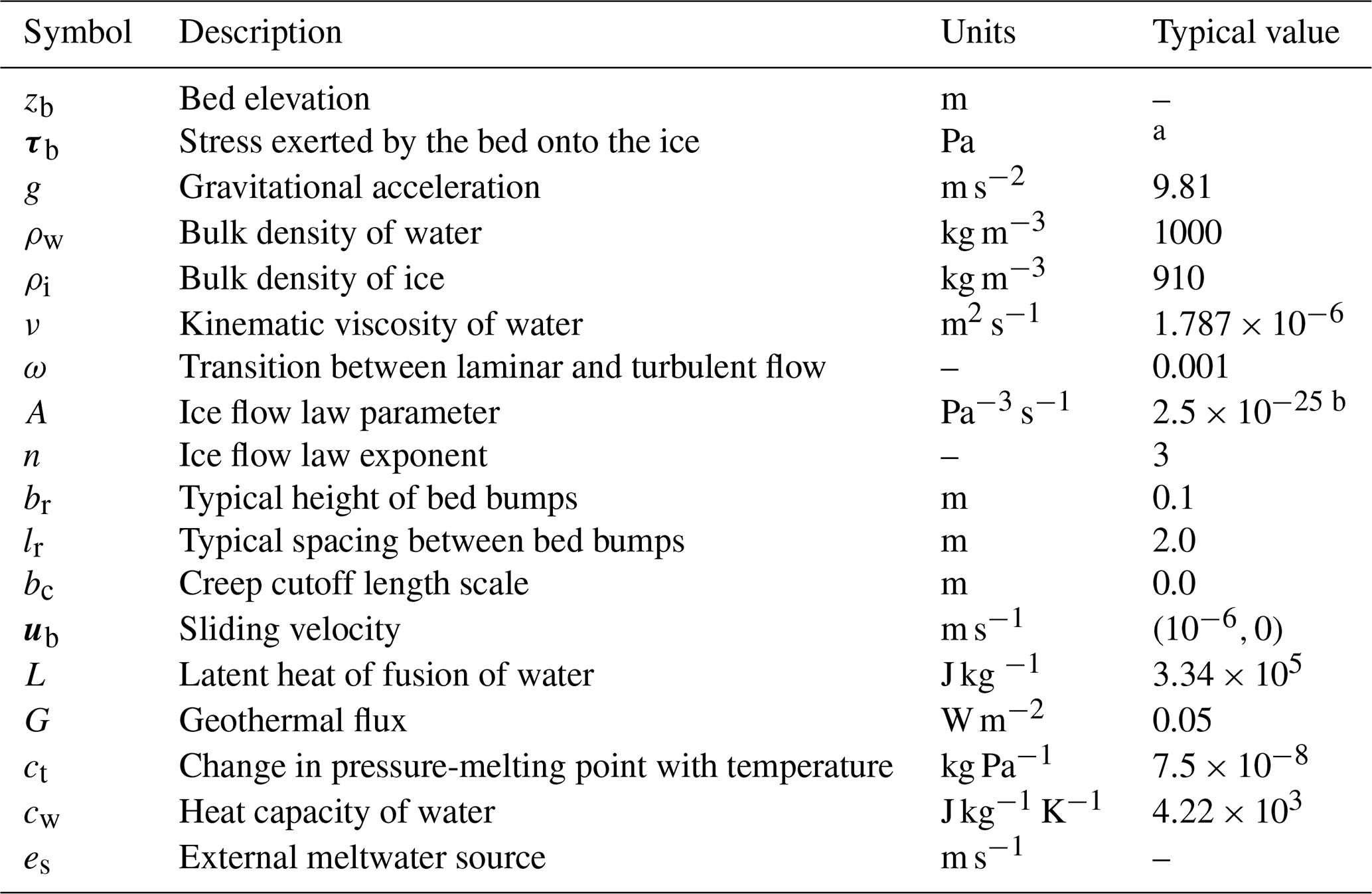
Table 1 List of constants and parameters employed in SUHMO. ^a The expression for the basal drag follows a modified Weertman law (Weertman, 1957): $C_{\mathrm{b}}{u}_{\mathrm{b}}^{\mathrm{2}}N$, where the value for C_b is typically set to 400 s² m⁻². ^b This value is chosen in accordance with a closure of the form AlNⁿ (de Fleurian et al., 2018).

2.3 Introduction of a diffusion term

As described in the introduction, the subglacial drainage system is made of various coexisting and dynamically evolving subglacial drainage structures. These are typically broken into two categories: distributed (or inefficient) flow structures and channelized (or efficient) flow structures. The advantage of this set of governing equations is that only one equation (i.e., Eq. 6) is necessary to model the drainage space, and this equation accommodates both inefficient and efficient elements. One drawback from Eq. (6), however, is that it was originally derived by considering a sheet drainage system, central to which is the growth of the water sheet thickness, while equations governing channel growth are intrinsically two-dimensional. In practice, adding a simple melt-opening term in Eq. (6) to accommodate channels causes the water sheet thickness to grow locally (e.g., in each computational cell), because the second dimension, the channel width, has been dropped from the problem formulation.

This behavior is not an issue if relatively coarse meshes are used in configurations where the primary interest is effective pressure fields, but it does prevent channel geometries from converging with mesh resolution. Convergence with mesh resolution is an important feature of consistent numerical methods; additionally, AMR requires consistent convergence with mesh resolution to be effective. As a first step towards addressing this issue, we modify Eq. (6) by adding a diffusion-like term as follows:

$$\begin{array}{}\text{(9)}& {\displaystyle \frac{\partial b}{\partial t}}={\displaystyle \frac{\dot{m}}{{\mathit{\rho }}_{\mathrm{i}}}}+\mathit{\beta }{u}_{\mathrm{b}}-A|P_{\mathrm{i}}-P_{\mathrm{w}}{|}^{n-\mathrm{1}}(P_{\mathrm{i}}-P_{\mathrm{w}})l_{\mathrm{c}}+\mathrm{\nabla }\cdot \mathcal{D}\mathrm{\nabla }b,\end{array}$$

where the diffusion coefficient depends on the dissipation term of the melt rate:

$$\begin{array}{}\text{(10)}& \mathcal{D}={\displaystyle \frac{b}{{\mathit{\rho }}_{\mathrm{i}}L}}(-{\mathit{\rho }}_{\mathrm{w}}g\mathit{q}\cdot \mathrm{\nabla }h+c_{\mathrm{t}}{c}_{\mathrm{w}}{\mathit{\rho }}_{\mathrm{w}}\mathit{q}\cdot \mathrm{\nabla }{P}_{\mathrm{w}}).\end{array}$$

With this formulation, we aim to represent melting of channel walls as heat dissipation is no longer limited to channel/cavity ceilings. Adding this diffusion term and neglecting englacial storage, Eq. (8) then becomes

$$\begin{array}{}\text{(11)}& \begin{array}{rl}\mathrm{\nabla }& \cdot \left[{\displaystyle \frac{-b^{\mathrm{3}}g}{\mathrm{12}\mathit{\nu }(\mathrm{1}+\mathit{\omega }\mathit{Re})}}\mathrm{\nabla }h\right]=\dot{m}[{\displaystyle \frac{\mathrm{1}}{{\mathit{\rho }}_{\mathrm{w}}}}-{\displaystyle \frac{\mathrm{1}}{{\mathit{\rho }}_{\mathrm{i}}}}]\\ & +A|P_{\mathrm{i}}-P_{\mathrm{w}}{|}^{n-\mathrm{1}}(P_{\mathrm{i}}-P_{\mathrm{w}})l_{\mathrm{c}}-\mathrm{\nabla }\cdot \mathcal{D}\mathrm{\nabla }b-\mathit{\beta }{u}_{\mathrm{b}}+e_{\mathrm{s}}.\end{array}\end{array}$$

3 Algorithm details

We solve Eqs. (9) and (11) on a hierarchy of block-structured, Cartesian meshes using a finite-volume discretization, facilitated by the Chombo framework (Adams et al., 2001–2021). We extend the Chombo toolbox to solve the nonlinear evolution equation for the hydraulic head implicitly using the full approximation scheme (Briggs et al., 2000). The resulting algorithm accuracy is second order in space and first order in time. For completeness, Appendix A gives a brief summary of the main features of our AMR framework. We adopt the notation used in several previous studies (Berger and Colella, 1989; Martin et al., 2008; Cornford et al., 2013; Parkinson et al., 2020), and the reader is referred to these prior publications for additional details. All that follows is specific to a two-dimensional application with an isotropic Cartesian mesh.

3.1 Full approximation scheme for variable-coefficient, nonlinear elliptic PDE

3.1.1 Multigrid methods

Multigrid (MG) methods are commonly employed to solve linear or nonlinear problems which can be expressed as

$$\begin{array}{}\text{(12)}& \mathcal{A}\left(u\right)=\mathcal{F}.\end{array}$$

If we denote by $\stackrel{\mathrm{̃}}{u}$ an approximation to the exact solution u of this problem, we can define the error e as $e=u-\stackrel{\mathrm{̃}}{u}$ and the residual r as $r=\mathcal{F}-\mathcal{A}\left(\stackrel{\mathrm{̃}}{u}\right)$. If 𝒜 is a linear operator, then we obtain the residual equation:

$$\begin{array}{}\text{(13)}& \mathcal{A}\left(e\right)=r,\end{array}$$

with which we can start a recursive process of “restricting” (averaging) the residual onto a coarser grid to solve for a coarse correction of the error that we then interpolate back (usually referred to as “prolongation”) to the fine grid (Briggs et al., 2000). For linear systems, multigrid is highly efficient and can be implemented using a matrix-free approach. It is also straightforward to extend to AMR mesh hierarchies (Martin and Cartwright, 1996).

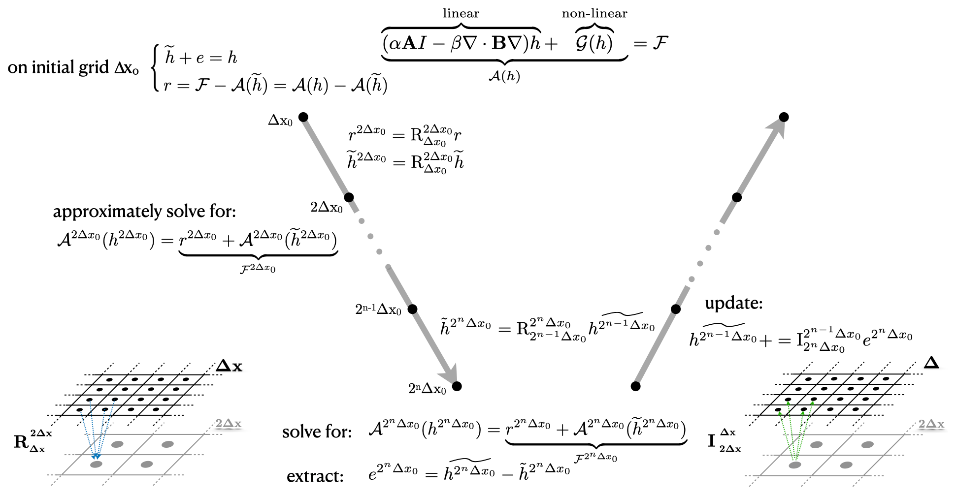
Figure 1 Illustration of one FAS MG iteration, following a V-cycle schedule of grids. See text for further explanations.

3.1.2 FAS multigrid

If 𝒜 is a nonlinear operator, we cannot make use of Eq. (13). Instead we use the residual in a new problem formulation:

$$\begin{array}{}\text{(14)}& \mathcal{A}\left(h\right)=r+\mathcal{A}\left(\stackrel{\mathrm{̃}}{h}\right),\end{array}$$

with which we can follow a similar recursive process to a traditional MG method. For completeness, the main steps of one FAS MG iteration are described here and illustrated in Fig. 1, focusing on the V-cycle scheduling of events; a more thorough description can be found elsewhere (Briggs et al., 2000; Henson, 2003). We have chosen to work with h instead of u to be consistent with our main variable – the hydraulic head. We will use the following general expression for the nonlinear operator 𝒜:

$$\begin{array}{}\text{(15)}& \mathcal{A}\left(h\right)=(\mathit{\alpha }\mathbf{A}I-\mathit{\beta }\mathrm{\nabla }\cdot \mathbf{B}\mathrm{\nabla })h+\mathcal{G}\left(h\right),\end{array}$$

where the nonlinear piece is contained in 𝒢(h). The restriction process is illustrated on the left of Fig. 1, by the arrow pointing down, while the prolongation is illustrated on the right with the arrow going up. The original level is labeled the finest level, and it has a mesh spacing of Δx₀. This level is coarsened n times by a factor of 2, so that coarsened grid n has a grid size of 2ⁿΔx₀.

We start by finding an approximate solution $\stackrel{\mathrm{̃}}{h}$ to the original problem Eq. (12) on the finest grid by using a few iterations of an iterative method (the relaxation method is described in Appendix B). The residual r is then evaluated, and both $\stackrel{\mathrm{̃}}{h}$ and r are averaged down to the first coarsened grid via a restriction operator denoted as $R_{\mathrm{\Delta }{x}_{\mathrm{0}}}^{\mathrm{2}\mathrm{\Delta }{x}_{\mathrm{0}}}$. We rewrite the problem as in Eq. (14) (where the new right-hand side – RHS – is denoted ${\mathcal{F}}^{\mathrm{2}\mathrm{\Delta }{x}_{\mathrm{0}}}$ in Fig. 1) and perform a number of relaxation iterations to find an approximate solution, $\stackrel{\mathrm{̃}}{h^{\mathrm{2}\mathrm{\Delta }{x}_{\mathrm{0}}}}$. This process is repeated until we reach the coarsest level. The coarsest error, $e^{{\mathrm{2}}^n\mathrm{\Delta }{x}_{\mathrm{0}}}$, can then be extracted from the solution and interpolated up to the next finer grid to be used to correct the local approximation $\stackrel{\mathrm{̃}}{h^{{\mathrm{2}}^{n-\mathrm{1}}\mathrm{\Delta }{x}_{\mathrm{0}}}}$ (see Fig. 1). This “prolongation” process is repeated, going up the levels until we reach the finest level again. We usually perform between two and four relaxation iterations while correcting the solution at each level.

3.1.3 Special treatment for the variable coefficient

We rewrite Eq. (11) to make it consistent with the operator that has been described in Fig. 1:

$$\begin{array}{}\text{(16)}& \begin{array}{rl}& \stackrel{\mathrm{linear}}{\overbrace{\mathrm{\nabla }\cdot \left[\stackrel{\mathbf{B}}{\overbrace{{\displaystyle \frac{-b^{\mathrm{3}}g}{\mathrm{12}\mathit{\nu }(\mathrm{1}+\mathit{\omega }\mathit{Re})}}}}\mathrm{\nabla }h\right]}}\\ & -\stackrel{\mathrm{nonlinear}}{\overbrace{A|P_{\mathrm{i}}-{\mathit{\rho }}_{\mathrm{w}}g(h-z_{\mathrm{b}}\left){|}^{n-\mathrm{1}}\right(P_{\mathrm{i}}-{\mathit{\rho }}_{\mathrm{w}}g(h-z_{\mathrm{b}}))l_{\mathrm{c}}}}\\ & =\stackrel{\mathrm{nonlinear}\mathrm{lagged}}{\overbrace{-{\displaystyle \frac{{\mathit{\rho }}_{\mathrm{c}}}{L}}{\mathit{\rho }}_{\mathrm{w}}g[\mathrm{1}-c_{\mathrm{t}}{c}_{\mathrm{w}}{\mathit{\rho }}_{\mathrm{w}}]\mathit{q}\cdot \mathrm{\nabla }h}}\\ & +{\displaystyle \frac{{\mathit{\rho }}_{\mathrm{c}}}{L}}(G+|{\mathit{u}}_{\mathrm{b}}\cdot {\mathit{\tau }}_{\mathrm{b}}|-c_{\mathrm{t}}{c}_{\mathrm{w}}{\mathit{\rho }}_{\mathrm{w}}^{\mathrm{2}}g\mathit{q}\cdot \mathrm{\nabla }{z}_{\mathrm{b}})\\ & -\mathrm{\nabla }\cdot \mathcal{D}\mathrm{\nabla }b-\mathit{\beta }{u}_{\mathrm{b}}+e_{\mathrm{s}},\end{array}\end{array}$$

where ${\mathit{\rho }}_{\mathrm{c}}=(\frac{\mathrm{1}}{{\mathit{\rho }}_{\mathrm{w}}}-\frac{\mathrm{1}}{{\mathit{\rho }}_{\mathrm{i}}})$. We discuss our treatment of the remaining nonlinearity and h dependencies in the RHS in Sect. 3.2. Note that the coefficient B is both spatially variable and a function of the primary variable h, via the coupling with Re. In our final implementation of the algorithm, B is recomputed on the finest grid at the beginning of every V cycle and then averaged down on all coarser grids. We experimented with fully lagging B, estimating the Reynolds number before the first V-cycle iteration and freezing its value for the remaining of the solve, but this resulted in poor overall algorithmic efficiency, as discussed in Appendix C.

3.2 Map of the algorithm

In order to solve the coupled set of Eqs. (9) and (16), we use a combination of FAS-MG iterations as described in Sect. 3.1 to solve for the hydraulic head and traditional MG to solve for the gap height. We note that the lagged term in Eq. (16), as well as any term involving the water flux, will depend on h in a non-trivial way. To ensure these are treated properly, we embed the FAS-MG solve for h in external Picard iterations (in which the value of the gap height is frozen). We have found that the required number of Picard iterations is, on average, typically one or two. This number can occasionally increase, particularly during transient phases.

We use a backward Euler method to discretize the temporal term in Eq. (9), reorganizing to be consistent with Eq. (12):

$$\begin{array}{}\text{(17)}& \stackrel{\mathcal{A}\left(b^{n+\mathrm{1}}\right)}{\overbrace{(I-\mathrm{\Delta }t\mathrm{\nabla }\cdot \mathcal{D}\mathrm{\nabla })b^{n+\mathrm{1}}}}=b^n+\mathrm{\Delta }t[{\displaystyle \frac{\dot{m}}{{\mathit{\rho }}_{\mathrm{i}}}}+\mathit{\beta }{u}_{\mathrm{b}}-A{N}^{\mathrm{3}}{l}_{\mathrm{c}}],\end{array}$$

where we have replaced the effective pressure (P_i−P_w) with N, and n=3 has been assumed.

The main steps required to advance our main variables from t=tⁿ to $t=t^{n+\mathrm{1}}$ are summarized in Algorithm 1. The superscripts n and k refer to the current time step and the current Picard iteration, respectively. For better readability, n is omitted when discussing Picard iterations. When relevant, “CC” will refer to cell-centered variables, while “FC” will refer to face-centered variables.

Following common usage (for example, in Martin and Colella, 2000), we enforce boundary conditions at domain boundaries and between AMR grid patches (both at the same refinement level and between levels) through the use of a ring of ghost cells (“GC”) around each logically rectangular patch.

Algorithm 1 Skeleton of a SUHMO time step ($t^n\to t^{n+\mathrm{1}}$).

(I) Start the time step

(a) Fill GC of hⁿ and bⁿ

(b) h_old←hⁿ and b_old←bⁿ

(II) Evaluate hⁿ⁺¹

while ! converged do

(a) h_lagged←h_k

(b) Compute $\mathrm{\nabla }{h}_k^{\mathrm{cc}/\mathrm{fc}}$ and $\mathrm{\nabla }{z_{\mathrm{b}}}_k^{\mathrm{cc}/\mathrm{fc}}$

(c) Re-q dependency

– Compute ${\mathit{Re}}_k^{cc}$ by solving the quadratic equation $\mathit{\omega }{\mathit{Re}}^{\mathrm{2}}+\mathit{Re}-\frac{b^{\mathrm{3}}g}{\mathrm{12}{\mathit{\nu }}^{\mathrm{2}}}\left(\right|\mathrm{\nabla }h\left|\right)=\mathrm{0}$

– Evaluate ${\mathit{Re}}_k^{\mathrm{fc}}$

– Update ${\mathit{q}}_k^{\mathrm{fc}}$ based on Eq. (2)

– Evaluate ${\mathit{q}}_k^{\mathrm{cc}}$

(d) Compute the external source term ${e_{\mathrm{s}}}_k$ based on the type of external water input (localized/distributed)

(e) Compute the RHS of Eq. (16)

– Update ${\dot{m}}_k$ using Eq. (5). All dot products are computed at FC before being interpolated to CC

– Evaluate the FC diffusive coefficient based on Eq. (10), 𝒟_k = f($\mathrm{\nabla }{h}_k^{\mathrm{fc}}$, $\mathrm{\nabla }{z_{\mathrm{b}}}_k^{\mathrm{fc}}$, ${\mathit{q}}_k^{\mathrm{fc}}$)

(f) Solve for h_k+1 (Eq. 16) using the FAS-MG method described in Sect. 3.1

(g) Average down and fill GC of h_k+1

(h) Check for convergence

if  $\frac{{∥h_{k+\mathrm{1}}-h_{\mathrm{lagged}}∥}_{\mathrm{\infty }}}{{∥h_{\mathrm{old}}∥}_{\mathrm{\infty }}}\le \mathit{ϵ}$ then

$h^{n+\mathrm{1}}\leftarrow h_{k+\mathrm{1}}$

converged = true

end if

end while

(III) Evaluate bⁿ⁺¹

(a) Re-evaluate $\mathrm{\nabla }{h}^{n+\mathrm{1},\mathrm{cc}}$, ${\mathit{Re}}^{n+\mathrm{1},\mathrm{cc}/\mathrm{fc}}$, ${\mathit{q}}^{n+\mathrm{1},\mathrm{cc}/\mathrm{fc}}$ based on hⁿ⁺¹

(b) Compute the RHS of Eq. (17)

– Update ${\dot{m}}^{n+\mathrm{1}}$ based on Eq. (5)

(c) Solve for bⁿ⁺¹ (Eq. 5) using a traditional MG method with a Gauss–Seidel relaxation method

– Re-evaluate 𝒟ⁿ⁺¹ using Eq. (10) and hold fixed during the solve

(IV) End the time step

(a) Write a plot/checkpoint file or perform post processing analysis

4 Analysis of the algorithm efficiency

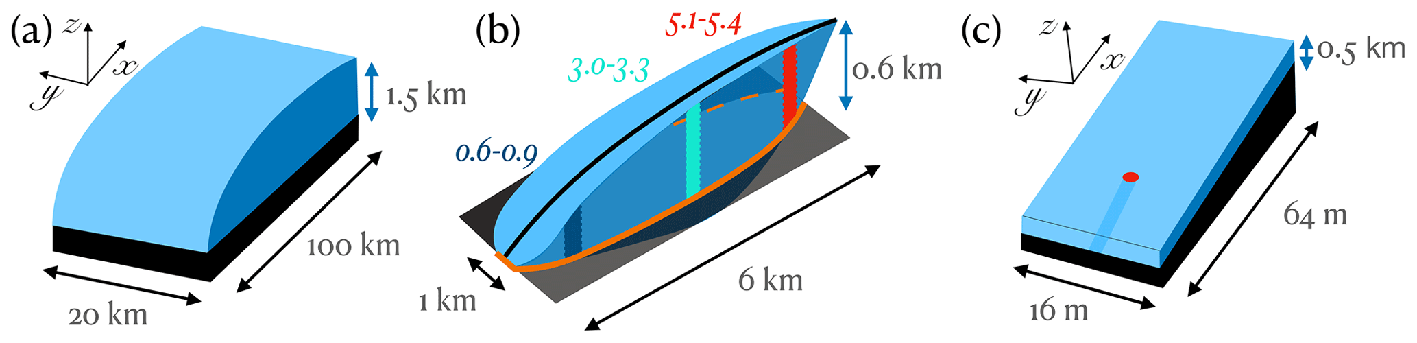
Figure 2 Panels (a) and (b) are sketches of synthetic glacier topographies used in SHMIP (de Fleurian et al., 2018): (a) 100 km-long ice sheet margin with a maximum thickness of 1500 m and (b) 6 km-long valley glacier with a 600 m altitude difference between summit and terminus. The orange region in panel (b) outlines the intersection of z_b=0 with the ice – note the bed overdeepening. Panel (c) is a sketch of the channelizing test case geometry used for convergence analysis. Note the thickness of the ice and the smaller horizontal spatial scale. The red dot shows the location of the moulin, which has a diameter of 1.5 m.

4.1 Distributed test case

We start by analyzing a simple distributed-flow test case. The topography considered is the synthetic representation of a land-terminating ice sheet margin from SHMIP (de Fleurian et al., 2018), illustrated in Fig. 2a. The ice sheet domain measures 100 km in the x direction and 20 km in the y direction, the bed is flat, and a parabolic ice surface z_s is prescribed by

$$\begin{array}{}\text{(18)}& z_{\mathrm{s}}(x,y)=\mathrm{6}(\sqrt{x+\mathrm{5000}}-\sqrt{\mathrm{5000}})+\mathrm{1}.\end{array}$$

In order to evaluate the convergence properties of the complete algorithm, we evolve the system to a fixed time with increasing resolution, halving Δx with each refinement. The solution error is then computed by comparing Φ^c, the solution at resolution Δx, with the finer solution ϕ^f computed using $\mathrm{\Delta }x/\mathrm{2}$ and averaged onto the coarser grid (Φ^f→c). The L² norm of the error for a simulation with n_tot cells is

$$\begin{array}{}\text{(19)}& {\text{Err}}_{L^{\mathrm{2}}}=\sqrt{{\displaystyle \frac{\mathrm{1}}{n_{\mathrm{tot}}}}\sum _{i=\mathrm{0}}^{n_{\mathrm{tot}}}({\mathrm{\Phi }}_{\mathrm{i}}^{\mathrm{c}}-{\mathrm{\Phi }}_{\mathrm{i}}^{\mathrm{f}\to \mathrm{c}}{)}^{\mathrm{2}}}.\end{array}$$

Figure 3a shows the error convergence using six grid resolutions for two variables of interest: h and N. The slope of the error demonstrates second-order convergence for both variables.

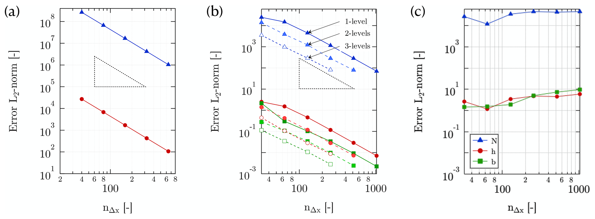
Figure 3 Convergence results for (a) the distributed test case, (b) the channelized test case with the diffusion term and (c) the original channelized test case without diffusion. The variables shown are the effective pressure (N) in blue, the head (h) in red and the gap height (b) in green. The x axis is the number of cells in the computational domain in the x direction, n_Δx.

4.2 Channelized test case

We now turn our attention to a channelizing test case. The domain is a rectangle of 64 m in the x direction by 16 m in the y direction. The bed is sloped in the x direction (with a +2 % slope) and is topped with a slab of ice of constant thickness everywhere (500 m). A moulin delivering 30 m³ s⁻¹ of water is located 16 m from the outlet of the domain in the x direction. The geometry is shown in Fig. 2c. Periodicity is assumed in the y direction, a homogeneous Dirichlet boundary condition (outlet) is prescribed at x=0 m, and a homogeneous Neumann boundary condition is prescribed at x=64 m. Note that the moulin source term follows a spatial Gaussian profile, as shown in the top plot of Fig. 4a – the convergence of which is exactly second order. Additionally, the moulin input is gradually increased in time, from 0 at time t=0 s to the maximum value after about a month, and the simulation proceeds until steady state is reached.

We use Eq. (19) to evaluate the convergence properties of SUHMO in this slightly more challenging test case. Results using seven grid resolutions are presented in Fig. 3b and c. The original formulation (Eqs. 6 and 8) fails to converge: as the resolution increases, the channel width becomes smaller and smaller, with the limit being the cell size Δx. This phenomenon is illustrated in the middle plot of Fig. 4a and in Fig. 4b for a simulation with Δx=0.125 m. In this case, the gap height is seen to exceed 12 m, a situation deemed unphysical in most cases, and we clearly observe that all the flow is routed through a single cell. As can be seen in Fig. 3b, adding the diffusion term to the formulation (Eqs. 9 and 16) enables second-order convergence of all the variables of interest. In this case, as is evidenced by the bottom plot of Fig. 4a and by Fig. 4b, the channel width can extend over several Δx and the overall shape and aspect ratio of the conduit better fit the idea of what a channel should be.

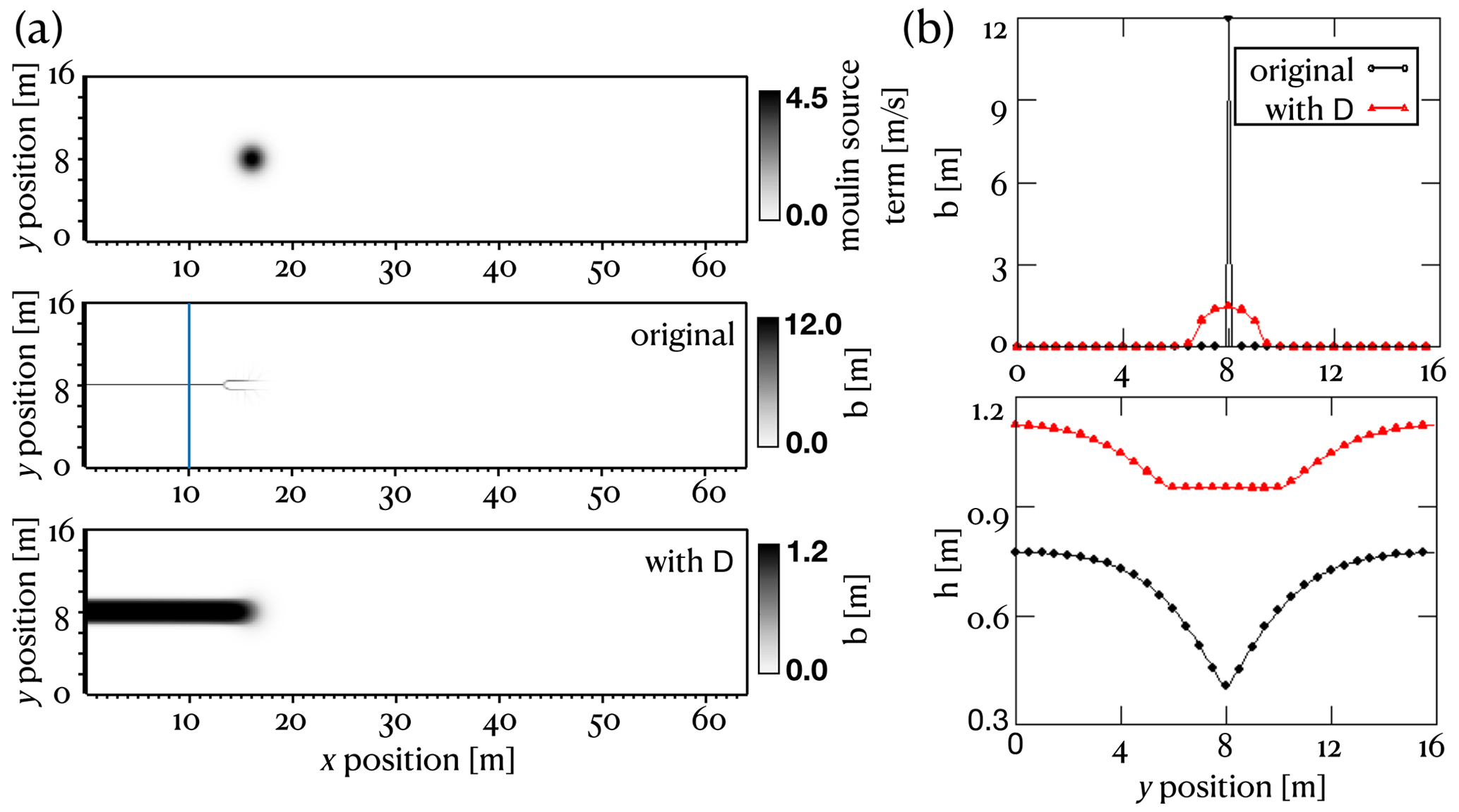
Figure 4 (a) Two-dimensional fields of moulin input and gap height (b) extracted from computations with mesh size Δx=0.125 m. (b) One-dimensional plots of gap height (b) and head (h) extracted from the two-dimensional fields, at location x=10 m, highlighted by the blue line in panel (a). Note that original refers to the formulation without the diffusion term, while with D refers to the formulation including the diffusion term.

To demonstrate our AMR implementation, we also perform a numerical convergence analysis using several levels of refinement. The AMR scheme should ideally produce solutions with comparable accuracy to a uniform mesh solution with the same (finest) resolution. Using the previously described test case, a refinement criterion based on the local melting rate enables refinement of the region where channelization occurs. Starting from a baseline, single-level simulation with a cell size of Δx, we enable the computation to continue and allow either one or two extra level(s) of refinement, where the finest level will have a cell size of either $\mathrm{\Delta }x/\mathrm{2}$ or $\mathrm{\Delta }x/\mathrm{4}$, respectively. This two- or three-level simulation is then compared to results at a finer resolution, $\mathrm{\Delta }x/\mathrm{4}$ or $\mathrm{\Delta }x/\mathrm{8}$, respectively. The results shown in Fig. 3b indicate that the error using two or three AMR levels is comparable to that of the single-level solution with the same effective resolution. The entire plot can be read horizontally, where an imaginary line drawn from a point on the one-level line should intersect the corresponding equivalent resolution on the two-level or three-level line, as is the case here.

5 SHMIP suite of test cases

Having demonstrated the convergence and efficiency of SUHMO, we turn our attention to a set of simple test cases from SHMIP (de Fleurian et al., 2018) to demonstrate the validity of our implementation. SHMIP is built around six synthetic suites of experiments (labeled from A to F), each consisting of a set of four to six numerical experiments designed to show the formation and evolution of the different drainage elements (sheets and channels) in the context of different input scenarios. Two geometries are considered, a land-terminating ice sheet margin and a synthetic valley glacier geometry, as shown in Fig. 2a and b, respectively. In the paper, the results from 13 different models are presented, including the SHAKTI model from Sommers et al. (2018).

We show steady-state cases (Suites A, B and E) in Sect. 5.1 and use Suite F in Sect. 5.2 to explore seasonal forcing. We compare all of our results to those obtained with SHAKTI (all results from the SHMIP project are open source and freely available online; see Werder et al., 2018). We believe that such comparisons are appropriate since SHAKTI is the closest in formulation to SUHMO, and so, by tuning to the same set of parameters and showing that we exhibit similar behavior, we hope to validate our approach. Note that the diffusion term is included in what follows, but its impact is negligible in these non-channelizing test cases. Additionally, the geothermal flux is not used in Suites A and B, in order to reach a steady state and retrieve the prescribed discharge, and the creep cutoff length scale b_c is always set to 0 so that the creep length scale l_c reverts to b (see Eq. 7), consistent with the SHAKTI contribution in de Fleurian et al. (2018). Finally, while Suite E has been designed in part to investigate the effect of bed slope on model predictions, we elected to turn off the pressure-melting contribution and focus on validating our implementation on this challenging geometry (our numerical implementation uses a structured, unskewed mesh). Results for Suite E with an added pressure-melting contribution are available in the Supplement.

5.1 Steady-state test cases

Results for the SHMIP test cases A, B and E are presented in Figs. 5, 6 and 7, respectively. The longitudinal evolution of the width-averaged effective pressure N is displayed on the left-hand side of all the figures. The right-hand side shows the total discharge and its various contributions to be compared with the total recharge. The discharge is the evolution along the x axis of the y integral of the face-centered water flux q^x, while the volumetric recharge contains contributions from both moulin input (when applicable) and melting. Using the notation introduced in Sect. A2, the discharge at each x_i location can be computed on the coarsest grid as

$$\begin{array}{}\text{(20)}& \text{dis}\left(x_i\right)=\sum _{\begin{array}{c}\mathit{p}\in (i,\mathbb{Z})\\ \mathit{p}\in {\mathrm{\Omega }}^{\mathrm{0},x}\end{array}}{\mathit{q}}_p^x\mathrm{\Delta }{x}^{\mathrm{0}},\end{array}$$

while the recharge is the cell-integrated right-hand side of Eq. 1):

$$\begin{array}{}\text{(21)}& \text{rech}\left(x_i\right)=\sum _{\begin{array}{c}\mathit{p}\in (i,\mathbb{Z})\\ \mathit{p}\in {\mathrm{\Omega }}^{\mathrm{0}}\end{array}}\left({\displaystyle \frac{{\dot{m}}_p}{{\mathit{\rho }}_{\mathrm{w}}}}+e_{\mathrm{s},p}\right)\mathrm{\Delta }{x}^{\mathrm{0}}\mathrm{\Delta }{x}^{\mathrm{0}}.\end{array}$$

At steady state, the recharge and discharge at the domain outlet should be exactly the same. Some figures also display efficient and inefficient contributions to the total discharge, which are computed based on a degree of channelization (DoC) variable. The DoC is a cell-centered variable used to quantify the relative contribution of the two ice-opening terms in the RHS of Eq. (9):

$$\begin{array}{}\text{(22)}& \text{DoC}={\displaystyle \frac{\frac{\dot{m}}{{\mathit{\rho }}_{\mathrm{i}}}}{\frac{\dot{m}}{{\mathit{\rho }}_{\mathrm{i}}}+\mathit{\beta }{u}_{\mathrm{b}}}},\end{array}$$

with values between 0 and 1 in each cell. A DoC close to 1 indicates a high degree of channelization, while a value close to 0 is indicative of a sheet-like drainage system. The efficient and inefficient contributions to the total discharge at x_i are expressed as dis(x_i)DoC(x_i) and dis(x_i)(1−DoC(x_i)), respectively.

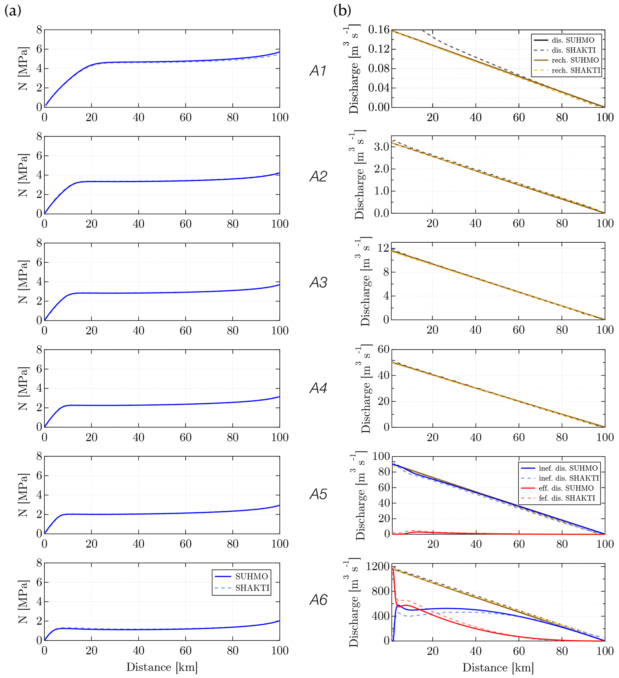
Figure 5 Steady-state results for the SHMIP suite of test cases A: (a) y-average evolution of effective pressure N with distance from the outlet and (b) volumetric discharge, to be compared to the total recharge the system receives (see text for further explanation). Cases A5 and A6 also display the contributions from the inefficient and efficient systems (their sum gives the total discharge). For validation purposes, results from SHAKTI (Sommers et al., 2018) as presented in de Fleurian et al. (2018) are also shown.

Suites A and B use the land-terminating ice sheet margin geometry (Fig. 2a). In Suite A, a steady and spatially uniform water input is prescribed, with total recharge increasing as we progress from A1 to A6. In Suite B, the same amount of water as in case A5 is fed into an increasing number of moulins (from 1 in B1 to a 100 in B5). For additional details on the parameterization of the different suites, the reader is referred to the online instructions (https://shmip.bitbucket.io/instructions.html, last access: 1 January 2023). Single-level (no AMR) simulations are performed, with a fixed cell size Δx⁰=312.5 m and a fixed time step dt=1 h, which is consistent with values reported from other two-dimensional models in de Fleurian et al. (2018). We apply a Dirichlet boundary condition h=z_b at the left edge (outlet) of the domain and Neumann boundary conditions with 0 prescribed flux on all other domain boundaries. The steady state is quickly reached in all cases, and simulations are run for approximately 400 d. Results obtained with SUHMO compare well to those obtained with SHAKTI, as expected since both models are built on the same set of equations. We note from Figs. 5b and 6b that SUHMO exhibits slightly smaller contributions from the efficient system in cases that display a hybrid flow configuration (see A6 in Fig. 5b, for example). These discrepancies are attributed to discretization differences between both models. SHAKTI uses an unstructured mesh, while SUHMO uses regular Cartesian meshes. We note that discretization features are probably the cause of the overshoot observed in Fig. 6b for case B1 with SHAKTI. The recharge provided by each moulin in Suite B is another potential source of inconsistency. In this study, a Gaussian distribution is assumed.

Suite E uses the synthetic valley glacier geometry (Fig. 2b). In this experiment, water input is uniformly distributed at the bed of the glacier. Here also, single-level simulations are performed, with Δx⁰=23.4375 m and dt=1 h. The boundary conditions are similar to those in Suites A and B. As already specified, the value of c_t is set to 0 for this suite of experiments (removing the pressure-melting term in Eq. 5). The steady state is quickly reached in all cases, and simulations are run for approximately 400 d. While the effective pressure distributions obtained using SUHMO compare well to those obtained using SHAKTI, we note bigger differences in the spatial distribution of the hybrid flow configuration in Fig. 7b. These are again attributed to differences in mesh and cell size between SUHMO and SHAKTI. We note the same tendencies as the over-deepening of the valley increases (from E1 to E5), however, with an increasingly sheet-like distribution throughout.

Figure 6 Steady-state results for the SHMIP suite of test cases B: (a) y-average evolution of effective pressure N with distance from the outlet and (b) volumetric discharge, to be compared to the total recharge the system receives (see text for further explanation). The contributions from the inefficient and efficient systems (their sum gives the total discharge) are also featured. For comparison, results from SHAKTI (Sommers et al., 2018) as presented in de Fleurian et al. (2018) are also shown.

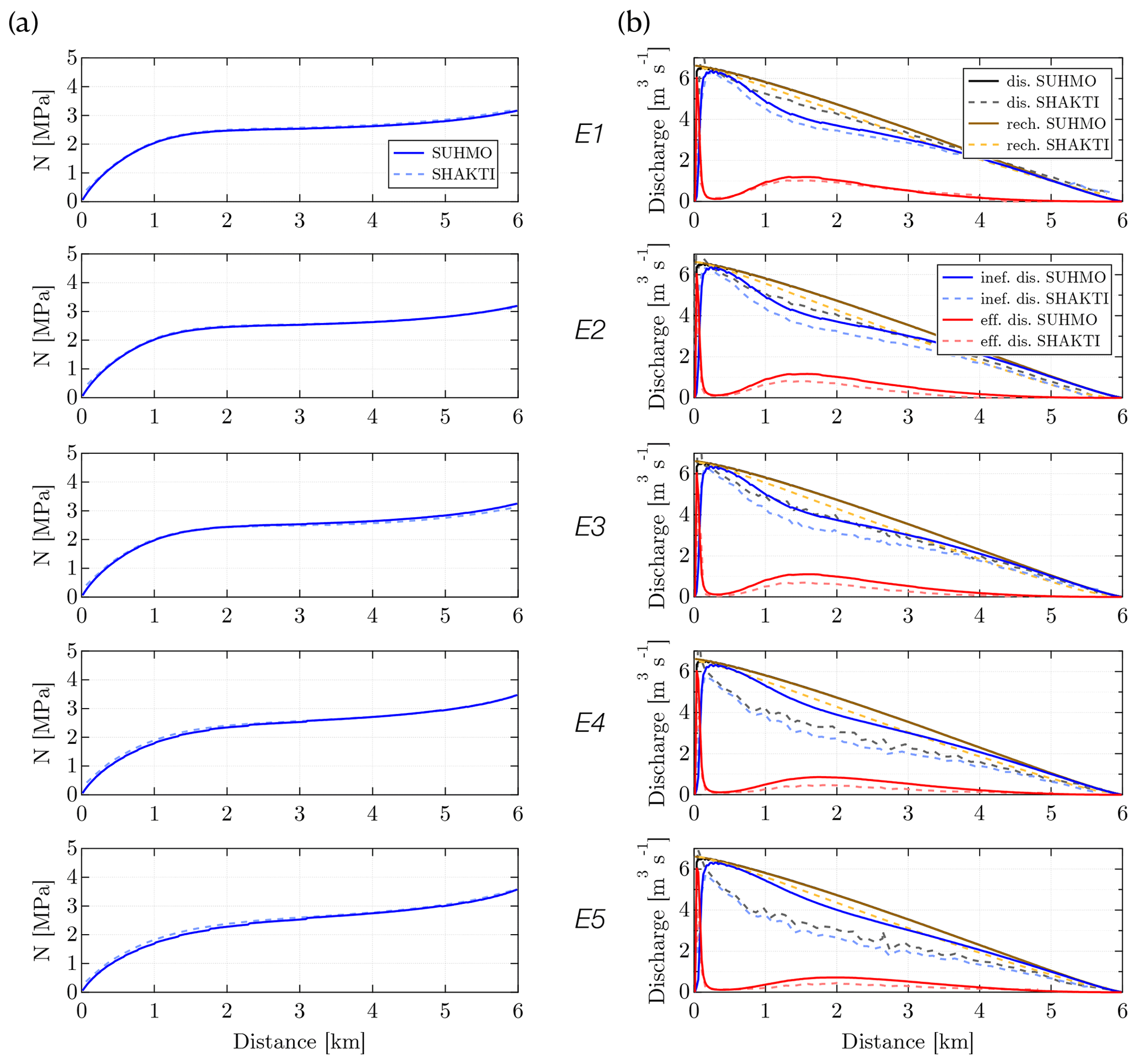
Figure 7 Steady-state results for the SHMIP suite of test cases E: (a) y-average evolution of effective pressure N with distance from the outlet and (b) volumetric discharge, to be compared to the total recharge the system receives (see text for further explanation). The contributions from the inefficient and efficient systems (their sum gives the total discharge) are also featured. For validation purposes, results from SHAKTI (Sommers et al., 2018) as presented in de Fleurian et al. (2018) are also plotted.

5.2 Suite F: seasonal cycle with valley topography

We turn our attention to SHMIP Suite F. The results presented in Sect. 5.1 focused on the effects of the geometry and water input type on otherwise steady-state configurations. Suite F prescribes a seasonal water forcing in the synthetic valley glacier geometry of case E1 (Bench Glacier reference geometry). The water input increases from run F1 to run F5, as can be seen in Fig. 8b. The setup follows that of Suite E. A total of 6 years are simulated, allowing sufficient time to settle into a periodic state. Year 6 results are presented in Fig. 8a. Time evolutions of the averaged effective pressure N are extracted at three locations of interest, labeled low, middle, and high bands, depicted in color in Fig. 2b. As before, results obtained with SUHMO closely follow those of SHAKTI.

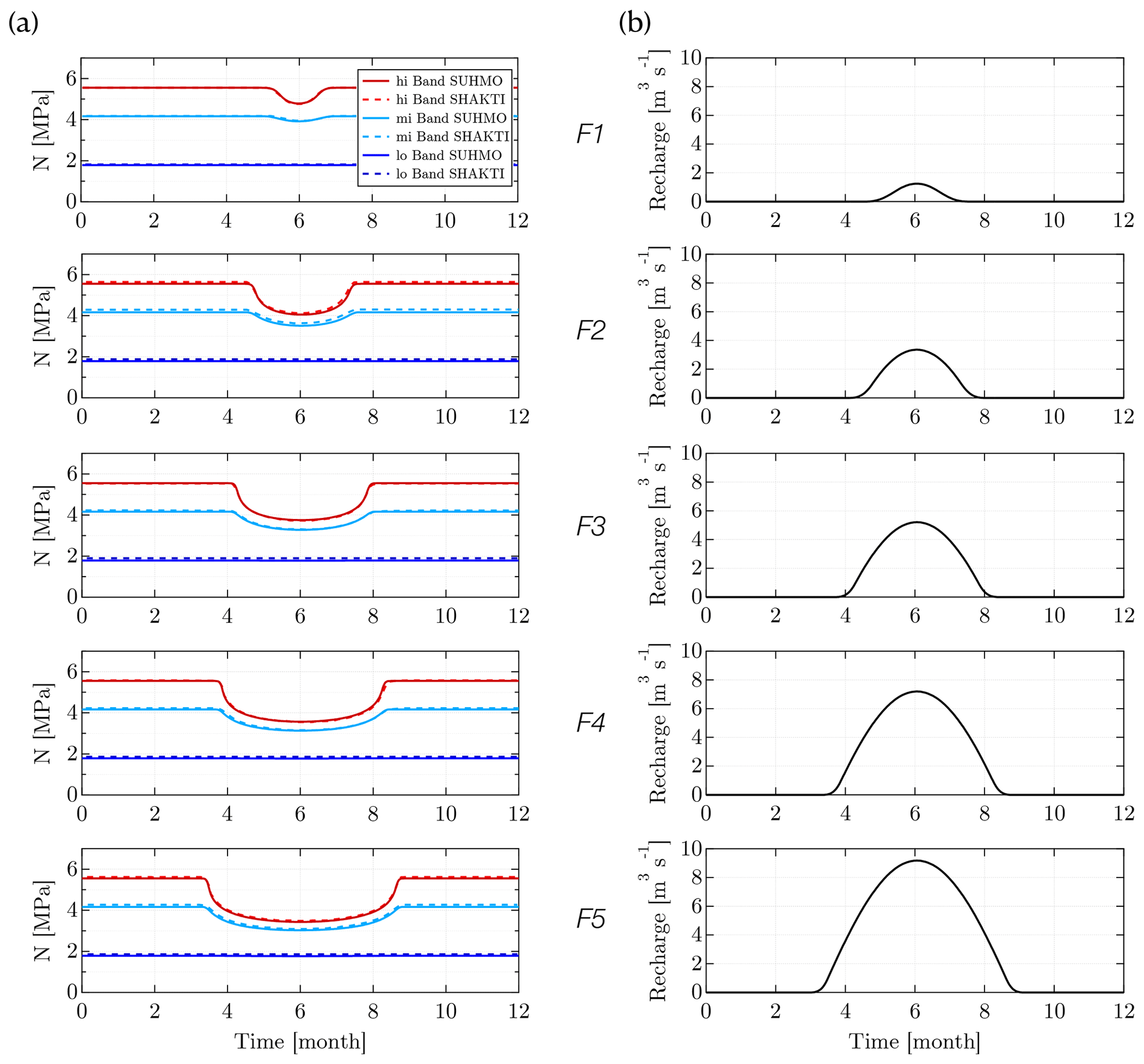
Figure 8 Steady-state results for the SHMIP suite of test cases F: (a) time evolution of the averaged effective pressure N at three locations of interest (see text and Fig. 2b) and (b) time evolution of the seasonal water forcing. For comparison, results from SHAKTI (Sommers et al., 2018) as presented in de Fleurian et al. (2018) are also shown.

Overall, while comparisons with SHMIP do not enable a true validation of our results, they do help validate our algorithm and provide an idea of how SUHMO compares to other subglacial hydrology models available in the literature.

6 AMR synthetic experiment

6.1 Case description

The test cases in Sect. 5 were all single-level experiments. In the present section, we now consider a synthetic square topography of 100 km by 100 km, generated with the intent of emulating catchment areas found at ice sheet margins. Both the bed geometry and ice thickness are shown in Fig. 9a. The bed height varies from 0 m to just under 1000 m, while the ice thickness increases from 100 m in the bottom-left corner (red dot location) to 700 m in the top-right corner. Zero flow via a homogeneous Neumann boundary condition is imposed on the two interior boundaries (y=0 and x=100 km), while Dirichlet boundary conditions are prescribed on the other two boundaries (with h=z_b, so that P_w=0).

Five runs will be presented hereafter – labeled from R₀ to R₄ (see Table D1), all using a base mesh with 256 cells in both the x and y directions. This value is chosen so Δx⁰=390.625 m, which is typical of many ice sheet simulations. The runs are forced by 63 randomly placed moulins, delivering a total water input of 5180 m³ s⁻¹. The location of the moulins is shown in Fig. 9b. We emphasize that the topography, moulin location and amount of water input used here have not been designed to reproduce an existing glacier area. The water delivered by the moulins is constant, no seasonal cycle is considered, and it is also quite high: this experiment should be taken as a demonstration of the robust behavior of the system even under prolonged high melting scenarios, when a high degree of channelization is expected. Our purpose is to demonstrate the importance of spatial resolution when looking at subglacial water patterns and ultimately to examine the impact of resolution on the effective pressure distribution.

All runs start from an established, steady-state, single-level simulation with no moulins. The moulins activate at t=0 s and the influx ramps up over a period of 2 months until the maximum is reached. The simulations are run for another 22 months after that, bringing the total simulated time to 2 years. The time step is dt=2 h in the first year before increasing to 5 h for the remainder of the simulation.

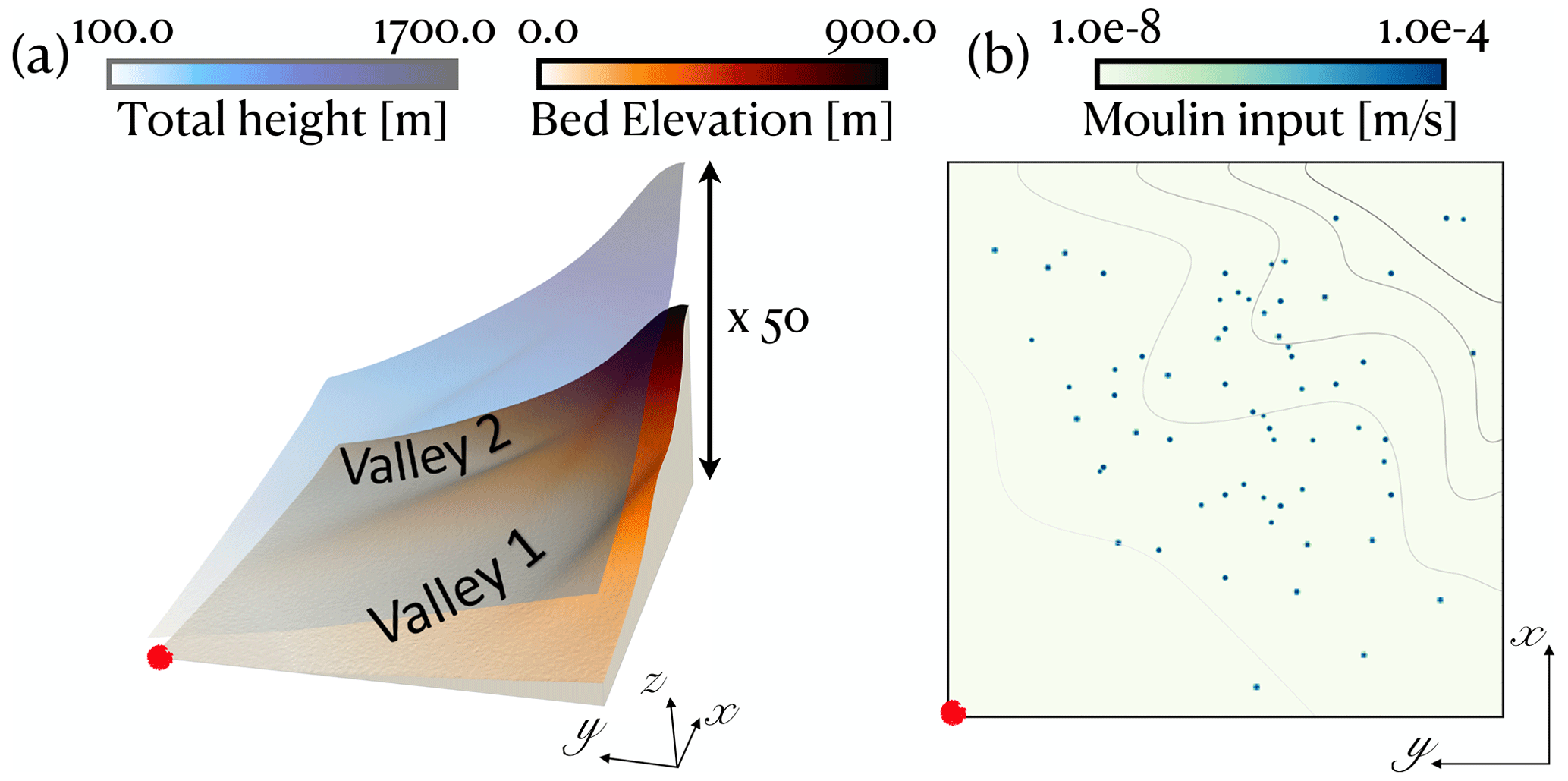
Figure 9 Synthetic square topography for runs R₀ to R₄: (a) extruded bed elevation (showing two valley regions) and ice height and (b) location of the moulins and isocontours of bed elevation. The red dot in both images shows the location of the lowest elevation – the outlet.

6.2 Overview of computational requirements

An example of mesh configuration for runs R₁ to R₃ is shown in Fig. 10b. In every case, a regridding operation is performed each simulated week, so that the dynamic meshing can follow the water patterns and add or remove refinement around the channels as they develop or retract. We use both the gap heights and melting rates to tag cells for refinement, for this example, cells in which the melt rate exceeds $\mathrm{2}\times {\mathrm{10}}^{-\mathrm{5}}$ kg m⁻² s⁻¹ are tagged for refinement, along with cells in which the gap height exceeds 0.1 m (this is effectively only active for R4, since the gap height is smaller for R3 and under). As can be seen, this criterion is very efficient, and only a small area of our entire computational domain ends up requiring up to four levels of refinement (due to the very small cell size reached, R₄ does not provide any additional visual insight and is therefore omitted from the figures).

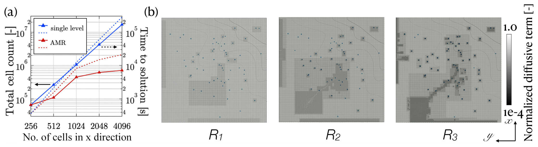
Figure 10 (a) Log–log plot of cell counts (plain lines with triangles) and execution times (dotted lines) versus resolution for the synthetic experiment and (b) example of mesh distribution for runs R₁ to R₃ overlayed on the locations of the moulins, normalized diffusive term (Sect. 2.3), and isocontours of bed elevation.

A single-level run with the same resolution as R₄ (4096×4096) would require evolving over 16 million cells, when 20 times fewer cells are required in the AMR run to capture what we believe to be most of the important features, as can be seen in Fig. 10a (the cell count in the AMR runs is obtained by averaging the total number of cells evolved over the course of the simulation). The total time to solution is also shown in Fig. 10a. For completeness, results from single-level simulations with resolution matching each finest level of refinement k of R_k are also reported. The total time to solution in this case does not scale exactly with the increase in resolution: the simulation contains a transient ramp up where moulins activate, and refining means creating more channels and spatial stiffness, as evidenced by the increasing number of FAS MG iterations (not reported here). The time-to-solution ratio of single level versus AMR simulations, however, increases with refinement and is well over an order of magnitude for the most refined case presented here. Additionally, note that despite being performed very frequently, the cost of regridding never accounts for more than 0.7 % of the total computational time.

6.3 Results and analysis of the effective pressure distribution

The first three rows of Fig. 11 show fields of gap height (b) and effective pressure (N) for runs R₀ and R₂ to R₄. A close-up on the valley 1 area (see Fig. 9) illustrates the extent and shape of the central channel. One interesting observation is that no channel forms in R₀; no channelization ever occurs, even if the simulation is extended for another 10 years. R₁ is very similar to R₀ in that no real channel inception can be seen and is therefore omitted in Fig. 11. This appears to demonstrate a “minimum resolution requirement” to capture channelization behavior in this example. Similar minimum resolution requirements were demonstrated for marine ice sheets in Cornford et al. (2016). Such a minimum resolution is, however, difficult to quantify in practice and may be case-dependent. More investigation (currently ongoing) is required to understand tendencies in resolution requirements, but a design criterion could be a much needed numerical tool.

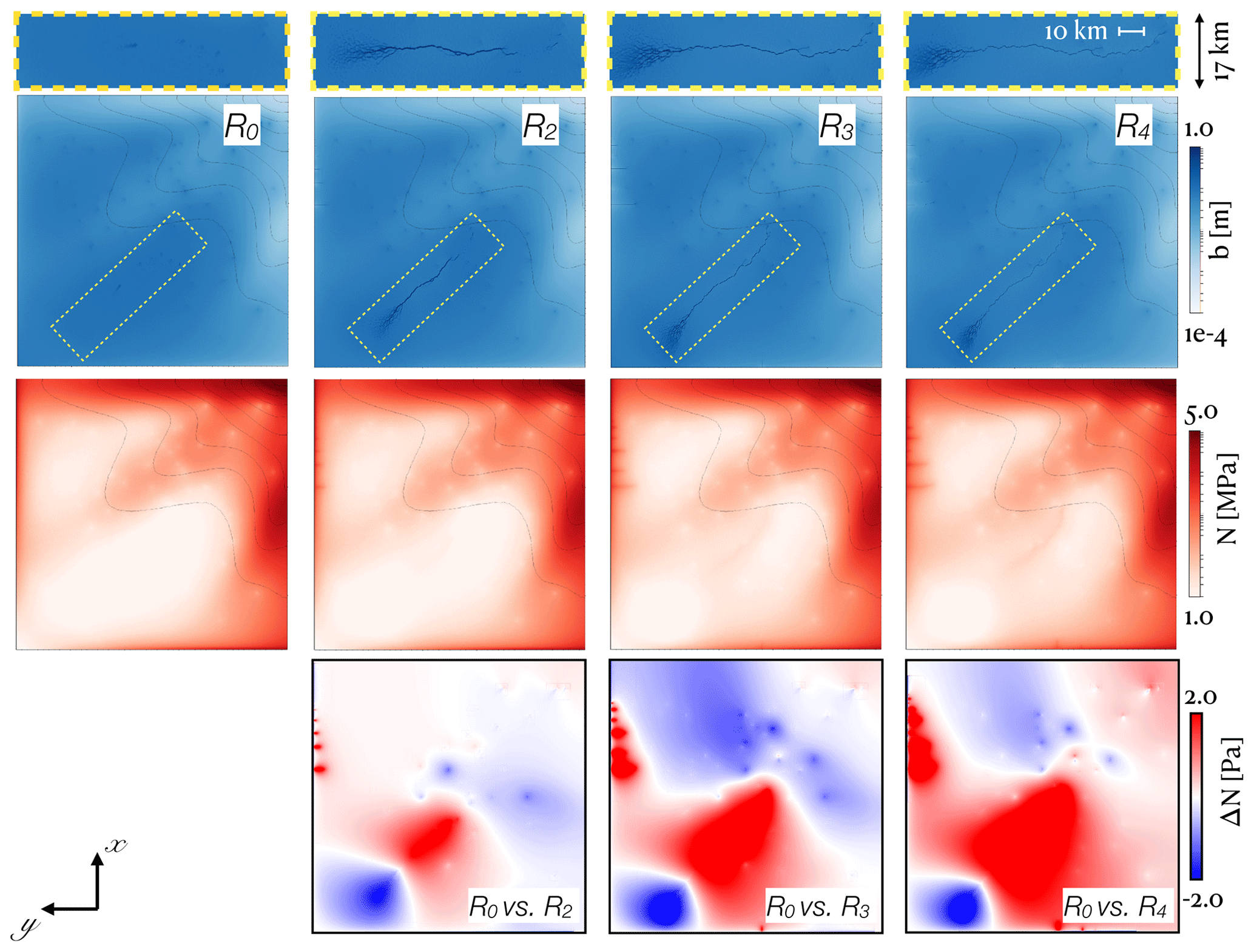
Figure 11 Fields of gap height (top two rows) and effective pressure (third row) for runs R₀ and R₂ to R₄, with overlayed isocontours of bed elevation. For each run, a close-up of the channelizing area in the valley 1 region (see Fig. 9) is also displayed. The bottom row shows fields of effective pressure differences between R₀ and R₂ to R₄, from left to right.

The bottom row of Fig. 11 displays differences in effective pressure (ΔN) between R₀ and, respectively, R₂, R₃ and R₄, from left to right. As expected, N increases significantly in the valley 1 area and near the top boundary (y=100 km) for $R_{k,k>\mathrm{1}}$, where channels are seen to develop. For R₃ and R₄, ΔN can reach up to 10 % of the global maximum of N and, more importantly, up to 25 % of the local N value (up to 0.6 MPa). These differences are deemed non-negligible in the context of evaluating a locally varying friction law, such as the ones from Schoof (2005) or Tsai et al. (2015). Figure 1 in Brondex et al. (2017), for example, shows strong nonlinearities in certain low-pressure regimes, where a difference of this order could result in very different basal drag profiles. Such sensitive areas are more likely to be located near the grounding line, where ice is thinner, and the potential impact on ice velocity warrants further investigation.

Note that all flow features may not be properly resolved in the present configuration. Indeed, even the run with the most AMR levels (R₄) still has a resolution of about 25 m (see Table D1), when channels are commonly believed to have a diameter of about 1–10 m. The extent to which channels need to be resolved to sufficiently account for their impact in a coupled subglacial hydrology–ice sheet modeling system is still an open question. For example, are friction law results sufficiently accurate when, say, differences of less than 5 % are observed in the N profile as the resolution is doubled (or a new AMR level is added)? Regardless, this suite of simulations demonstrates that commonly used resolutions (on the order of 300–500 m) can sometimes fail to even reveal channelized features.

7 Concluding remarks

In this paper, we present and validate a novel AMR subglacial hydrology model, SUHMO, based on the Chombo framework (Adams et al., 2001–2021). We solve equations similar to those in Sommers et al. (2018), with the addition of a pseudo-diffusion to recover the wall melting in channels that was discarded in the derivation of the original equations. We demonstrate the usefulness of this additional term in achieving consistent spatial convergence as finer resolution begins to resolve flow configurations. Our algorithm uses an efficient combination of nonlinear MG iterations embedded in external Picard iterations. We show that results with SUHMO closely follow those obtained with SHAKTI (Sommers et al., 2018) on a broad selection of the SHMIP suite of test cases (de Fleurian et al., 2018). A more complex, multi-level test case is also presented which hints at the need for sufficient spatial resolution to correctly resolve subglacial system dynamics; computational performance analysis demonstrates the efficiency of AMR on such large-scale hydrologic problems when compared to a single-level run with the same spatial discretization. The AMR approach will eventually enable better ice-bed boundary conditions for ice sheet simulations at a reasonable computational cost.

With that in mind, future work will focus on the coupling of SUHMO with the BISICLES AMR ice sheet model (Cornford et al., 2013) in order to further investigate the sensitivity of model predictions to spatially accurate modeling of basal conditions. Indeed, while the precise topography of the subglacial network is generally deemed unimportant to the overall ice sheet dynamics, there is to our knowledge no real numerical proof of this assessment, and the results presented here allude to the potential impact of the finer resolution of these systems. A numerical tool capable of resolving the structure of channels, following them as they emerge and disappear, will be an asset in helping to determine whether this is indeed the case. The efficiency provided by AMR can also be leveraged if and when it is determined that sufficient resolution in specific regions is important.

Appendix A: AMR structure and notation

A1 Proper nesting

Calculations are performed on a hierarchy of ℓ_max nested, cell-centered level domains. For each AMR level $\mathrm{\ell }=\mathrm{0},\mathrm{\dots },{\mathrm{\ell }}_{\max }$, the problem domain Ω^ℓ is discretized by a uniform Cartesian grid Γ^ℓ with grid spacing Δx^ℓ. Level 0 is the coarsest level, encompassing the entire geometry, while each subsequent finer level, ℓ+1, is a factor $n_{\mathrm{ref}}^{\mathrm{\ell }}=\frac{\mathrm{\Delta }{x}^{\mathrm{\ell }}}{\mathrm{\Delta }{x}^{\mathrm{\ell }+\mathrm{1}}}$ finer than level ℓ ($n_{\mathrm{ref}}^{\mathrm{\ell }}$ is a power of 2, usually 2). Each Ω^ℓ is constructed from one or more rectangular subsets of Γ^ℓ, as can be seen in Fig. A1a: Ω¹, for example, is built from two separate rectangular blocks, each with their own subgrid ${\mathrm{\Gamma }}^{\mathrm{\ell },*}$. An important property is that each domain level is properly nested; that is, no interfaces exist between Ω^ℓ and Ω^ℓ±2, only between two subsequent levels or the domain boundary.

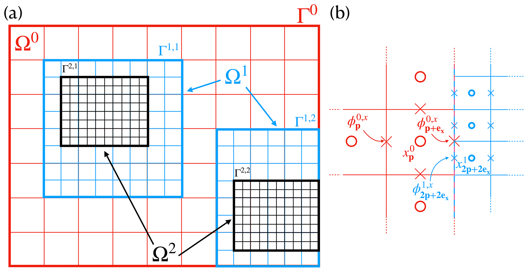
Figure A1 (a) Example of a block-structured mesh composed of three levels. Discrete-level domain Ω⁰ comprises the cell centers of the coarsest grid, Γ⁰. Level domains Ω¹ and Ω² are each built from two separate rectangular blocks, each with their own separate grids. (b) Focus on the coarse–fine interface between Ω⁰ and Ω¹. Locations of cell- and face-centered data are represented with circles and crosses, respectively. Face-centered data belonging to Ω^0,x on the interface are replaced by averaging of Ω^1,x (finer) data.

Certain derived quantities, such as fluxes, are located on two supplementary hierarchies of face-centered level domains that will be denoted Ω^ℓ,x and Ω^ℓ,y for x- and y-centered faces, respectively, on level ℓ.

A2 Cell- and face-centered data

Variables can be cell-centered or face-centered. We define a grid vector, p∈ℤ², choosing to number cells starting at (0, 0), and grid basis vectors ${\mathit{e}}_x=(\mathrm{1},\mathrm{0})$ and ${\mathit{e}}_y=(\mathrm{0},\mathrm{1})$. Cell centers within Ω^ℓ are then located at ${\mathit{x}}_p^{\mathrm{\ell }}=\mathrm{\Delta }{x}^{\mathrm{\ell }}(\mathit{p}+\frac{\mathrm{1}}{\mathrm{2}}({\mathit{e}}_x+{\mathit{e}}_y\left)\right)$ and the midpoints of cell faces within ${\mathrm{\Omega }}^{\mathrm{\ell },*}$ at ${\mathit{x}}_p^{\mathrm{\ell }}\pm \frac{\mathrm{\Delta }{x}^{\mathrm{\ell }}}{\mathrm{2}}{\mathit{e}}_{*}$. Cell-centered level variables ${\mathit{\varphi }}_p^{\mathrm{\ell }}=\mathit{\varphi }\left({\mathit{x}}_p^{\mathrm{\ell }}\right)$ and face-centered level variables ${\mathit{\varphi }}_p^{\mathrm{\ell },*}=\mathit{\varphi }({\mathit{x}}_p^{\mathrm{\ell }}-\frac{\mathrm{\Delta }{x}^{\mathrm{\ell }}}{\mathrm{2}}{\mathit{e}}_{*})$ follow naturally. Notice that ${\mathit{\varphi }}_p^{\mathrm{\ell },x}$ is located on the “western” face of the cell p and that ${\mathit{\varphi }}_p^{\mathrm{\ell },y}$ is located on the “southern” face of the cell p.

A3 Coarsening operator

We identify cells at different levels which occupy the same geometric regions by means of the coarsening operator ${\mathcal{C}}_r\left(\mathit{p}\right)=\frac{\mathit{p}}{r}$ and its inverse, the refinement operator. In that sense, ${\mathcal{C}}_r^{-\mathrm{1}}\left(\mathit{p}\right)$ is the set of all cells in a grid r times finer that represent the same geometric region (in a finite-volume sense) as the cell p (Martin and Colella, 2000).

A4 Composite variables

Discrete representations of continuous fields are then cell- and face-centered composite variables ϕ^comp, made up of “valid” (or uncovered by a finer level) portions of the level variables. First, level domains Ω^ℓ are divided into valid (${\mathrm{\Omega }}_{\mathrm{valid}}^{\mathrm{\ell }}$) and invalid (${\mathrm{\Omega }}_{\mathrm{invalid}}^{\mathrm{\ell }}$) regions, such that ${\mathrm{\Omega }}_{\mathrm{valid}}^{\mathrm{\ell }}={\mathrm{\Omega }}^{\mathrm{\ell }}-{\mathcal{C}}_{n_{\mathrm{ref}}^{\mathrm{\ell }}}\left({\mathrm{\Omega }}^{\mathrm{\ell }+\mathrm{1}}\right)$. Valid level domains for face-centered quantities are defined in the same way, ${\mathrm{\Omega }}_{\mathrm{valid}}^{\mathrm{\ell },*}={\mathrm{\Omega }}^{\mathrm{\ell },*}-{\mathcal{C}}_{n_{\mathrm{ref}}^{\mathrm{\ell }}}\left({\mathrm{\Omega }}^{\mathrm{\ell }+\mathrm{1},*}\right)$. A composite variable is then defined on the union of all valid regions, $\mathbf{\Omega }={\bigcup }_{\mathrm{\ell }}{\mathrm{\Omega }}_{\mathrm{valid}}^{\mathrm{\ell }}$, where ${\mathit{\varphi }}^{\mathrm{comp}}\left(\mathbf{\Omega }\right)={\bigcup }_{\mathrm{\ell }}{\mathit{\varphi }}^{\mathrm{comp}}\left({\mathrm{\Omega }}_{\mathrm{valid}}^{\mathrm{\ell }}\right)$. Likewise, composite vector fields are valid on all faces not overlain by finer faces.

We also construct ghost regions ${\mathrm{\Omega }}_{\mathrm{ghost}}^{\mathrm{\ell }}$ that surround Ω^ℓ. These usually contain one or two extra cells and exist purely for numerical convenience – to compute gradients or other face-centered quantities. These buffer regions contain either boundary-specified values or are used to store extrapolated data or data calculated by interpolation from valid regions of a coarser level. Details pertaining to the computation of composite operators such as gradients and Laplacians can be found in prior publications (Martin and Colella, 2000).

A5 Level variables – averaging down

It is sometimes necessary to transfer information from finer grids to coarser ones: ${\mathcal{C}}_{n_{\mathrm{ref}}^{\mathrm{\ell }}}\left({\mathrm{\Omega }}^{\mathrm{\ell }+\mathrm{1}}\right)$ is typically filled from appropriate cell-centered (or face-centered) arithmetic averaging of level ℓ+1 data. An example case is illustrated in Fig. A1b: where levels 0 and 1 meet, face-centered quantity ${\mathit{\varphi }}_{\mathit{p}+\mathrm{1}}^{\mathrm{0},x}$ would be replaced by $\frac{{\mathit{\varphi }}_{\mathbf{2}\mathbf{p}+\mathbf{2}{\mathbf{e}}_{\mathbf{x}}}^{\mathrm{1},x}+{\mathit{\varphi }}_{\mathbf{2}\mathbf{p}+\mathbf{2}{\mathbf{e}}_{\mathbf{x}}+{\mathbf{e}}_{\mathbf{y}}}^{\mathrm{1},x}}{\mathrm{2}}$.

A6 Regridding

We regrid every n_regrid time step. n_regrid is typically fixed at the beginning of a run. During this process, the solution at each grid cell and on each level, whether valid or currently covered, is tested against some specified criteria (or combination thereof) to determine whether refinement is required, in which case the cell is tagged for refinement. A new set of grids is then generated to ensure all tagged cells are covered by a finer level whilst still satisfying the rules introduced above regarding proper nesting. This procedure enables the refinement or coarsening of the grids over time, following regions of interest. The appropriate refinement criteria vary depending on the type of application. In the case of SUHMO, we typically refine based on high values of the melting rate and/or gap height to ensure we resolve the channelization process.

Appendix B: Relaxation method in the FAS-MG algorithm

To relax Eq. (14) on each FAS level, we employ nonlinear Gauss–Seidel method with multicolor ordering. With the formulation of Eq. (15) for the nonlinear operator, and using the notation introduced in Sect. A, we obtain the following discretized equation for each p cell on a given level where the notation ℓ has been omitted:

$$\begin{array}{}\text{(B1)}& \begin{array}{rl}& \mathit{\alpha }{\mathbf{A}}_p{h}_p\\ & +{\displaystyle \frac{\mathit{\beta }}{\mathrm{\Delta }{x}^{\mathrm{2}}}}\left[{\mathbf{B}}_{p+e_x}^x\right(h_{p+e_x}-h_p)-{\mathbf{B}}_p^x(h_p-h_{p-e_x})\\ & +{\mathbf{B}}_{p+e_y}^y(h_{p+e_y}-h_p)-{\mathbf{B}}_p^y(h_p-h_{p-e_y})]\\ & +\mathcal{G}\left(h_p\right)={\mathcal{F}}_p,\end{array}\end{array}$$

which can be rewritten as ℋ(h_p)=0, where

$$\begin{array}{}\text{(B2)}& \begin{array}{rl}\mathcal{H}\left(h_p\right)& =\mathit{\alpha }{\mathbf{A}}_p{h}_p\\ & +{\displaystyle \frac{\mathit{\beta }}{\mathrm{\Delta }{x}^{\mathrm{2}}}}\left[{\mathbf{B}}_{p+e_x}^x\right(h_{p+e_x}-h_p)-{\mathbf{B}}_p^x(h_p-h_{p-e_x})\\ & +{\mathbf{B}}_{p+e_y}^y(h_{p+e_y}-h_p)-{\mathbf{B}}_p^y(h_p-h_{p-e_y})]\\ & +\mathcal{G}\left(h_p\right)-{\mathcal{F}}_p.\end{array}\end{array}$$

Equation (B2) can be solved by resorting to Newton's method (for a scalar):

$$\begin{array}{}\text{(B3)}& h_p\leftarrow h_p-{\displaystyle \frac{\mathcal{H}\left(h_p\right)}{{\mathcal{H}}^{\prime }\left(h_p\right)}},\end{array}$$

where

$$\begin{array}{}\text{(B4)}& {\mathcal{H}}^{\prime }\left(h_p\right)=\mathit{\alpha }{\mathbf{A}}_p-{\displaystyle \frac{\mathit{\beta }}{\mathrm{\Delta }{x}^{\mathrm{2}}}}({\mathbf{B}}_{p+e_x}^x+{\mathbf{B}}_p^x+{\mathbf{B}}_{p+e_y}^y{\mathbf{\text{B}}}_p^y)+{\mathcal{G}}^{\prime }\left(h_p\right).\end{array}$$

Appendix C: A case for the treatment of the B coefficient in the FAS-MG algorithm

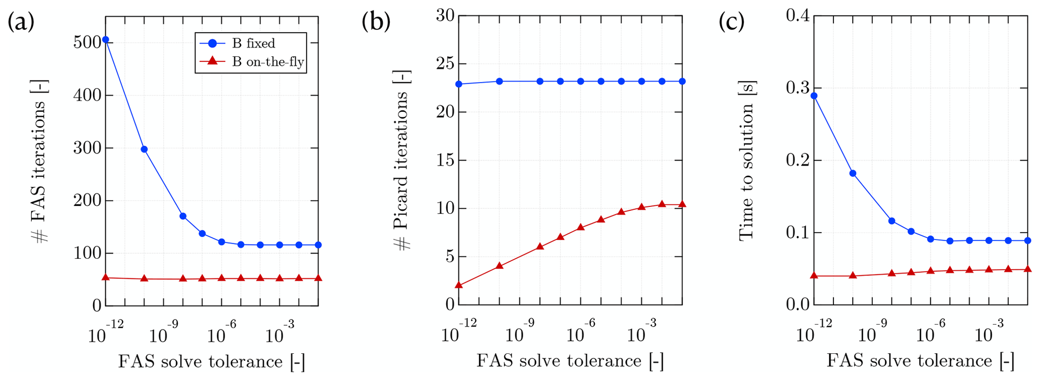
Figure C1 Average of the (a) number of FAS iterations, (b) number of Picard iterations and (c) total computational time required to complete one time step with SUHMO as a function of the FAS solve tolerance. The tolerance of the Picard iterations is held fixed at 10⁻⁸.

As mentioned in Sect. 3.1.3, the variable coefficient in the PDE Eq. (16) requires special treatment due to coupling with the main variable h. We tested two different approaches for the treatment of B. In the first, which we will call B fixed, the value of B is evaluated once per Picard iteration and is frozen during the FAS solve. With the second approach, which we will call B on the fly, B is recomputed and averaged down on each MG grid at the beginning of each V cycle. We investigate the overall efficiency of the algorithm in terms of the number of Picard and total FAS iterations and CPU time as a function of the FAS solve tolerance. While keeping the (relative) tolerance of the outer Picard solver at a constant value of 10⁻⁸, statistics are collected for about 20 time steps in a transient simulation (using the channelized test case described in Sect. 4.2), and the average per time step is presented in Fig. C1. Across the entire range of FAS tolerances considered, B on the fly is found to be more efficient, with a lower average number of FAS iterations per step and smaller computational time (albeit by a smaller margin due to the small computational overhead of recomputing B and updating the FAS multigrid hierarchy). When using the B fixed approach, tight FAS tolerances lead to a large increase in the average FAS iteration count without having a significant effect on the Picard iteration count. In contrast, B on the fly leads to a significant reduction of the Picard iteration count, because part of the nonlinearity is handled by the FAS.

Based on these results, we opt to use the B on the fly approach for all of our computations, and we fix the FAS tolerances to 10⁻¹⁰, appearing to provide a good compromise in terms of computational time.

Appendix D: Details of runs R₀ to R₄

Table D1 Details of the five AMR runs R_n.