the Creative Commons Attribution 4.0 License.
the Creative Commons Attribution 4.0 License.
 | 14 Jul 2023
Segmentation of XCO2 images with deep learning: application to synthetic plumes from cities and power plants
Joffrey Dumont Le Brazidec
Pierre Vanderbecken
Alban Farchi
Marc Bocquet
Jinghui Lian
Grégoire Broquet
Gerrit Kuhlmann
Alexandre Danjou
Thomas Lauvaux
Under the Copernicus programme, an operational CO2 Monitoring Verification and Support system (CO2MVS) is being developed and will exploit data from future satellites monitoring the distribution of CO2 within the atmosphere. Methods for estimating CO2 emissions from significant local emitters (hotspots; i.e. cities or power plants) can greatly benefit from the availability of such satellite images that display the atmospheric plumes of CO2. Indeed, local emissions are strongly correlated to the size, shape, and concentration distribution of the corresponding plume, which is a visible consequence of the emission. The estimation of emissions from a given source can therefore directly benefit from the detection of its associated plumes in the satellite image.
In this study, we address the problem of plume segmentation (i.e. the problem of finding all pixels in an image that constitute a city or power plant plume). This represents a significant challenge, as the signal from CO2 plumes induced by emissions from cities or power plants is inherently difficult to detect, since it rarely exceeds values of a few parts per million (ppm) and is perturbed by variable regional CO2 background signals and observation errors. To address this key issue, we investigate the potential of deep learning methods and in particular convolutional neural networks to learn to distinguish plume-specific spatial features from background or instrument features. Specifically, a U-Net algorithm, an image-to-image convolutional neural network with a state-of-the-art encoder, is used to transform an XCO2 field into an image representing the positions of the targeted plume. Our models are trained on hourly 1 km simulated XCO2 fields in the regions of Paris, Berlin, and several power plants in Germany. Each field represents the plume of the hotspot, with the background consisting of the signal of anthropogenic and biogenic CO2 surface fluxes near to or far from the targeted source and the simulated satellite observation errors.
The performance of the deep learning method is thereafter evaluated and compared with a plume segmentation technique based on thresholding in two contexts, namely (1) where the model is trained and tested on data from the same region and (2) where the model is trained and tested in two different regions. In both contexts, our method outperforms the usual segmentation technique based on thresholding and demonstrates its ability to generalise in various cases, with respect to city plumes, power plant plumes, and areas with multiple plumes. Although less accurate than in the first context, the ability of the algorithm to extrapolate on new geographical data is conclusive, paving the way to a promising universal segmentation model trained on a well-chosen sample of power plants and cities and able to detect the majority of the plumes from all of them. Finally, the highly accurate results for segmentation suggest the significant potential of convolutional neural networks for estimating local emissions from spaceborne imagery.
- Article
(14594 KB) - Full-text XML
-
Supplement
(351 KB) - BibTeX
- EndNote


Under the Paris Agreement on Climate Change, progress on emission reduction efforts is monitored on the basis of regular updates of the national greenhouse gas (GHG) inventories (UNFCCC, 2015). To independently assess the progress of countries towards their targets, objective means of tracking anthropogenic CO2 emissions and their evolution is needed. Top-down estimates based on atmospheric measurements can provide such observation-based evidence. Developed through the European Earth observation programme, Copernicus, the CO2 emissions Monitoring and Verification Support capacity (CO2MVS) will provide an operational emissions monitoring system based on such an approach (Janssens-Maenhout et al., 2020). It will operate in particular on a constellation of dedicated CO2 imaging satellites, the Copernicus CO2 Monitoring (CO2M) mission, as part of the Sentinel programme, which will be launched from the year 2026.
One aim of CO2MVS is to provide estimates of local emissions from hotspots such as cities or power plants that account for a major fraction of anthropogenic CO2 releases. For this purpose, local data assimilation can be applied to individual plumes visible in satellite CO2 images. A plume is defined as an increase in CO2 concentration above the background level that is caused by emissions from a hotspot. To estimate emissions from the plume, it is essential to detect it on satellite images. Thus, the detection of a plume, i.e. the identification of its contour, in a satellite image is a critical step in the evaluation of source emissions.
The detection and identification of pollutant plumes from simulated fields or observations has been the subject of an important amount of research. Lauvaux et al. (2022) exploit satellite images sampled by the TROPOspheric Monitoring Instrument (TROPOMI) to identify very large emitters of CH4, using a thresholding technique. Finch et al. (2022) successfully trained neural networks (NNs) on satellite images of NO2 to detect the presence of plumes. Recent thresholding techniques have proven effective in detecting large CO2 plumes in satellite images, by either using the Orbital Carbon Observatory-2 (OCO-2; Crisp et al., 2017; Reuter et al., 2019) or observing system simulation experiments (OSSEs; Kuhlmann et al., 2019a).
Nevertheless, the detection and quantification of CO2 plumes in satellite images remains a challenge with various obstacles. Conventional threshold-based methods rely on the signal-to-noise ratio of a plume. The signal is the CO2 enhancement inside the plume above the background field, and the noise is the variability in the measurements due to single sounding precision of the instrument and the interference of other anthropogenic and biospheric fluxes. Kuhlmann et al. (2019a) showed that for the expected single sounding precision of the CO2M (Copernicus Carbon Dioxide Monitoring mission) CO2 product (<0.7 ppm; 2 km resolution; swath width > 250 km; MRDv3), the signal-to-noise ratio of many cities and power plants is too small for a reliable detection of CO2 plumes with threshold-based methods. CO2M will overcome this limitation through an additional nitrogen dioxide (NO2) instrument on the same platform that, as a proxy to CO2, significantly improves plume detection capabilities (Kuhlmann et al., 2019a). CO2M will also provide CH4 observations (https://www.eoportal.org/satellite-missions/co2m, last access: 10 July 2023). However, not all currently planned CO2 imaging satellites (such as CO2Image; Butz et al., 2022) will have NO2 observations available, which puts a limit on the capabilities of the CO2 imaging instrument to detect emission plumes using threshold-based methods.
Although mainly motivated by CO2MVS, this study focuses on CO2 images in general. The objective is to cope with the signal-to-noise ratio (SNR) problem in CO2 plume detection problems, with the help of deep learning methods (Chollet, 2017; Zhang et al., 2022). In particular, we rely on convolutional neural networks (CNNs) to segment plumes more accurately than thresholding techniques by learning and capturing plume-specific spatial patterns. Plumes may indeed have certain spatial properties or shapes that can be exploited by an algorithm capable of extracting and learning these features. The image dataset used to train and test the CNN model is based on fields of column-averaged dry air mole fractions of CO2 (XCO2), simulated in the vicinity of the targeted sources (Grand Paris, Île-de-France (IdF), Berlin, and various power plants). Each image is comprised of (at least) a targeted source plume and the other nearby biogenic and anthropogenic fluxes, plus the instrumental noise typical of the sensor on board CO2M. Clouds are not included in the CO2 images for simplicity. They will be addressed in a separate publication.
A large amount of labelled data is a prerequisite for the use of CNNs. In Sect. 2, we present the two synthetic datasets that are used to train and evaluate the performance of the CNNs. The plume segmentation problem is then mathematically defined in Sect. 3.1. The loss function, which defines what the CNN should target, i.e. what a plume is according to the deep learning model, is described in Sect. 3.2. Next, in Sect. 3.3, the architecture and parameterisation of the CNN are introduced and explained. Subsequently, the trained model is applied in the following two contexts:
-
a context of geographical generalisation, where a model trained to recognise plumes on images from the regions of Paris, Berlin, and various power plants is evaluated on new images from the same regions, and
-
a context of geographical extrapolation, where a model trained to recognise plumes on images from the regions of Paris and various other power plants is evaluated on images from the region of Berlin.
In both cases, the CNN method is compared for reference to the thresholding plume segmentation method described by Kuhlmann et al. (2019a, 2021), which is available as part of a Python package for data-driven emission quantification (ddeq; https://gitlab.com/empa503/remote-sensing/ddeq, last access: 10 July 2023). Finally, conclusions on the performances of the deep learning models in these situations are provided.
2.1 Simulation of the CO2 fields
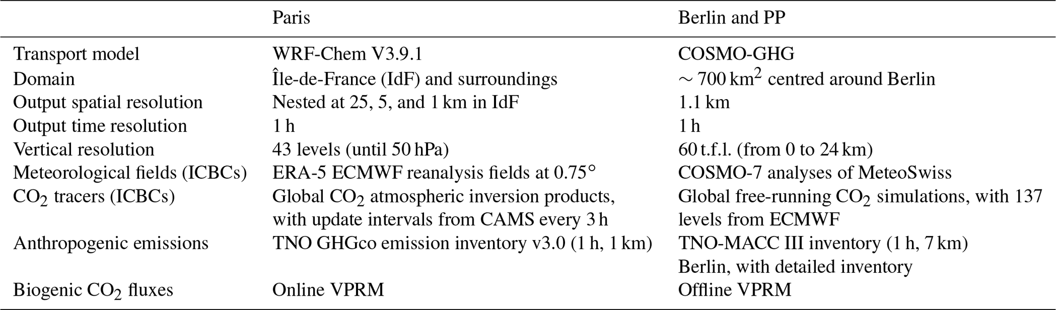
Two different atmospheric transport models are used to simulate the CO2 fields which provide the XCO2 images. Simulations in the Paris region by WRF-Chem V3.9.1 (Grell et al., 2005) are based on the configuration of Lian et al. (2021), while simulations in the Berlin region, including neighbouring power plants, are taken from the SMARTCARB project (Kuhlmann et al., 2019b; Brunner et al., 2019).
Paris data consist of 3-month meteorological and CO2 transport simulations on a nesting of three domains with different spatial resolutions (25, 5, and 1 km). Initial and boundary conditions (ICBCs) are forced with ERA-5 reanalysis fields (Hersbach et al., 2020) at a resolution of 0.75∘ for the meteorological simulations and Copernicus Atmosphere Monitoring Service (CAMS) 3 h update interval global CO2 atmospheric inversion products for the CO2 simulations (Chevallier, 2018). High-resolution inventories, the TNO GHGco v3.0 TNO-MACC_II and the VERIFY D2.1 v1.0 (Denier van der Gon et al., 2021), are used to simulate CO2 concentrations over the entire domain. Finally, biogenic fluxes are computed with the Vegetation Photosynthesis and Respiration Model (VPRM) model (Mahadevan et al., 2008) coupled online with the WRF-Chem V3.9.1 model.
The SMARTCARB simulations were run with the Consortium for Small-scale Modelling (COSMO)-GHG model for a domain centred on Berlin and covering several neighbouring power plants (Jänschwalde, Lippendorf, Boxberg, and others). The simulations were used to generate synthetic CO2M observations (Kuhlmann et al., 2020b) and to assess different plume detection and inversion methods (Kuhlmann et al., 2019a, 2020a, 2021; Hakkarainen et al., 2022). The model fields consist of hourly data over 1 year, with a spatial resolution of 0.01∘ and 60 vertical layers from 0 to 24 km. MeteoSwiss COSMO-7 analyses are used as the meteorological initial and boundary conditions, while the CO2 boundary conditions correspond to the fields of the ECMWF (European Centre for Medium-Range Weather Forecasts) free-running global CO2 simulations with 137 levels (Agustí-Panareda et al., 2014). Biogenic CO2 fluxes are modelled offline with the VPRM diagnostic biosphere model (Mahadevan et al., 2008). Finally, the TNO-MACC III inventory (Kuenen et al., 2014) is used for modelling anthropogenic emissions in most of the regions. Berlin emissions, however, are modelled with the help of a detailed inventory (Kuhlmann et al., 2019b). The main configuration parameters are summarised in Table 1.
Table 1Main set-up parameters of the transport of CO2 for the Paris simulations and the SMARTCARB simulations. Note that PP stands for power plant, and t.f.l. is for terrain-following layers.
2.2 Parameterisation of the CO2 field simulations
CNN segmentation models are trained and tested on fixed-size images, and XCO2 images of 160×160 pixels are extracted from the Paris and SMARTCARB datasets. Therefore, the images used to train and evaluate the CNN are not synthetic CO2M observations but a simplified dataset. The images are extracted such that the hotspot is located in the centre of the image, and the chosen size ensures that most of the hotspot plume is present in the image. The native resolution of 1.1 km of the SMARTCARB data is maintained during this extraction phase, while the Paris data are mapped from the original 200 pixels in longitude and 165 pixels in latitude to 160×160 pixels; the new image concentrations are calculated by cubic spline interpolation (Virtanen et al., 2020), which gives images with a resolution of 1.25×1.03 km2 in IdF.
A wide variety of fields and plumes are needed to train an efficient plume segmentation model. The dataset diversity and size is achieved through the following:
-
seasonal variability (January, March, and August for the Paris data to cover summer and winter; a whole year for SMARTCARB).
-
geographical variability (Paris; various locations in Germany).
-
emission range variability across different locations and times. In Berlin, the average emissions that are based on the inventory is 16.8 Mt yr−1, with a standard deviation (SD) of 7.2 Mt yr−1. In Jänschwalde, the emissions average is 33.3 Mt yr−1, with a SD of 7.7 Mt yr−1, while in Boxberg, the emissions average is 19.0 Mt yr−1, with a SD of 4.4 Mt yr−1. The Grand Paris emissions average is 20.7 Mt yr−1, with a SD of 9.5 Mt yr−1.
-
plume type variability, with single power plant plumes (a single major anthropogenic plume on the image) with Lippendorf, multiple plumes (several major anthropogenic plumes in the image) with Jänschwalde or Boxberg, cities (Grand Paris and Berlin), or cities with an extended suburb (Île-de-France (IdF), including the Paris region). The Paris data are split into two parts to assess the ability of the CNNs to retrieve plumes from the Paris conurbation alone (Grand Paris) or from the entire Paris region (IdF).
To fully account for the detectability factors affecting the SNR, the satellite instrumental noise must be taken into account. In this study, a Gaussian random noise, without spatial correlation, of 0.7 ppm (parts per million), typical of CO2M (Meijer, 2020), is used and added to the simulated XCO2 fields. Considering these various factors, the generation of a XCO2 image can be summarised in three steps, namely the simulation of the hotspot anthropogenic plume, the addition of the simulated background (biogenic and other anthropogenic fluxes), and the addition of the instrument noise. This is illustrated in Fig. 1.
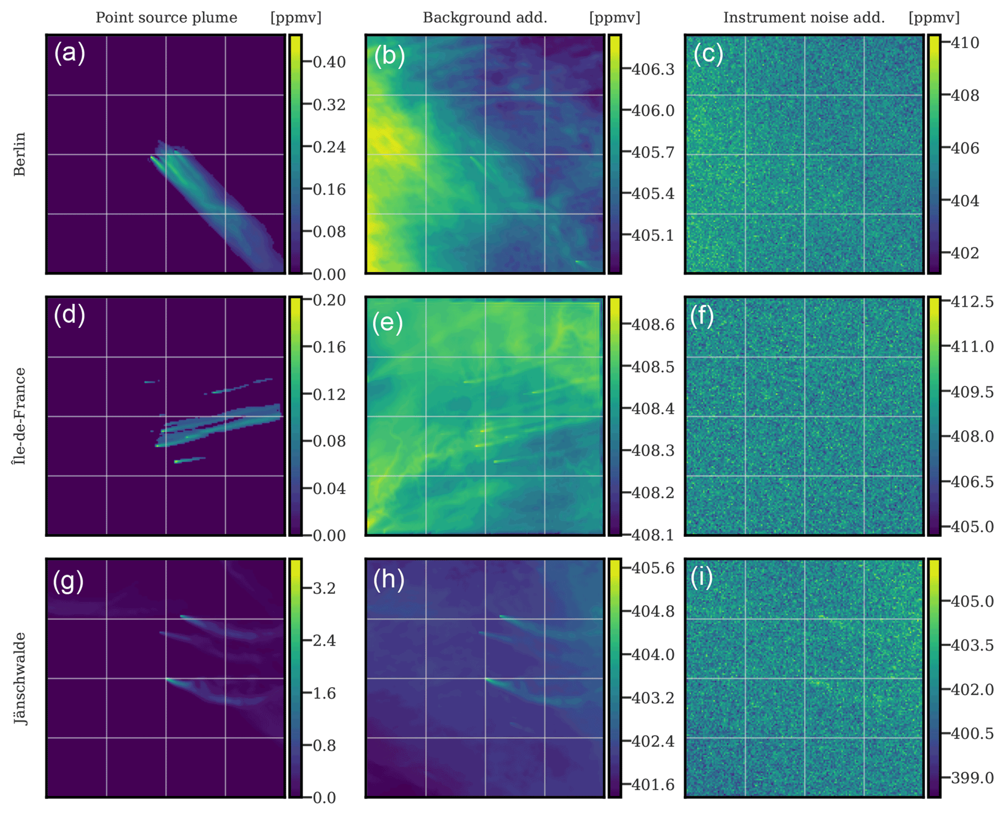
Figure 1Examples for the construction of three simulated XCO2 satellite images. Each row shows the generation of a sample XCO2 image, and three hotspots are considered at random times and days. Berlin (a–c). Paris (d–f). Jänschwalde (g–i) is located near other power plants, which explains the presence of multiple plumes. The left column displays the anthropogenic hotspot plumes with the concentrations in parts per million by volume (ppmv) indicated on the colour bars. In the middle column, the addition of background (biogenic and anthropogenic fluxes) is shown. Finally, in the right column, the full simulated image used as input to the CNN model with the addition of satellite instrument noise is revealed.
We provide the CNN model with full noisy images (right panels in Fig. 1), and we design it to return the plume masks of the hotspot plumes (left panels in Fig. 1).
Data augmentation techniques (Chollet, 2017) are applied to the training data. The training images are randomly shifted, zoomed, sheared, flipped, and rotated variants of the original images. Specifically, each image used for training the CNN has been subject to the following:
-
a random horizontal and vertical shift of 0 % to 20 % (the border values are then used to fill the missing values of the new image, as shown in Fig. 2);
-
a random zoom of 0 % to 20 %;
-
a potential horizontal or vertical flip, with a probability of 0.5;
-
a random rotation of 0 to 180∘; and
-
a random shear, i.e. a distortion along an axis (while the other axis is fixed) of 0 to 45∘.
Data augmentation is meant to (i) raise the performance of the CNN model, where data augmentation artificially and substantially increase the number of training data, thus reducing the risk of overfitting, and (ii) raise the representativeness of our plume database through the enforcement of geometrical invariance.
Figure 2 shows two examples of data-augmented fields and associated plumes.
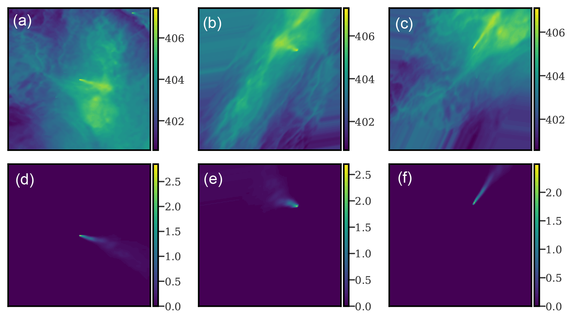
Figure 2Examples of augmented XCO2 fields (a–c; without instrumental noise) and corresponding plumes (d–f). The left column corresponds to the original XCO2 field and plume. The middle and right columns correspond to the same XCO2 fields, after shearing, flipping, rotating, and translating operations are complete. These are typical examples of what is used as input to the CNN model.
The selection of the data augmentation techniques used and their characteristics was based on experimentation. The extrapolation or distortion of the plumes due to data augmentation can lead to non-physical plumes. Yet, we empirically found that the use of such plumes improves the ability of the CNN model to segment real plumes.
3.1 Problem description
The plume segmentation problem can be defined, for a given image, as the detection of all pixels composing the plume.
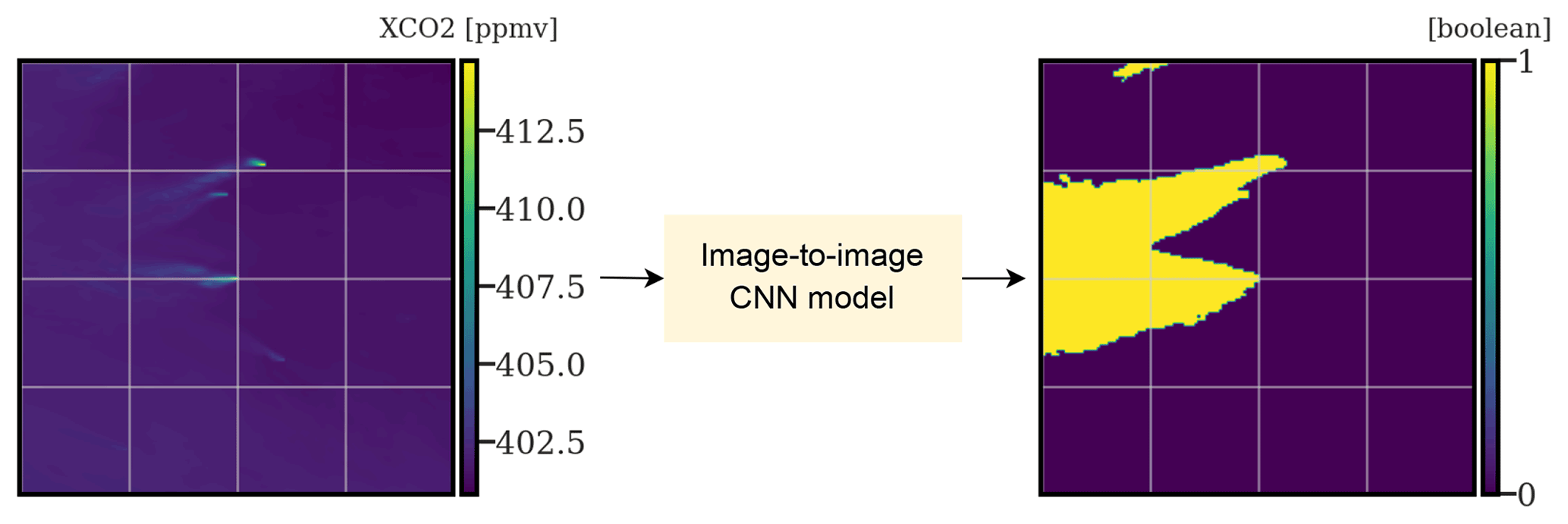
Figure 3Illustrating the principle of plume segmentation. An image-to-image model (here, a CNN) is used to extract the anthropogenic plumes from a XCO2 field for one or several hotspots.
This problem can be seen as an image-to-image problem, where the goal is to translate the original image into a Boolean map in which pixels are assigned to categories of either “true” (part of a hotspot plume) or “false” (not part of a hotspot plume), as shown in Fig. 3. Many algorithms can be designed to perform such a translation. However, in this study, we dispose of a labelled dataset as both the input XCO2 field and the corresponding targeted plume are available. In this context of supervised learning, for image processing, CNNs are particularly effective (Chollet, 2017; Zhang et al., 2022).
These algorithms are based on learning specific patterns of increasing complexity using smaller and simpler patterns (the filters). The larger and more complex patterns are specific to the learned targets (here, the plumes from the targeted sources). The filters are optimised to allow the learning of these complex target-specific features. This optimisation is done automatically, unlike most algorithms, where the filters would have to be chosen manually (feature engineering).
The CNN decomposes as a training step (which includes validation) and a test step. In the training step, the selected CNN model, described in Sect. 3.3, is trained with XCO2 field and Boolean map pairs. The Boolean map is composed of pixels equal to 1 if the pixel has a positive XCO2 concentration corresponding to the simulated anthropogenic plume or 0 if the pixel does not. For a given XCO2 field, the CNN model knows the target Boolean plume and learns to output a probability map that best matches it (supervised learning). The shapes of the input and output are equal, and each pixel in the output represents the probability that the pixel in the input belongs to the anthropogenic plume. In the testing step, the CNN model is applied to new input images, none of which has been seen during the learning phase, to assess its ability to generalise to new data.
3.2 Loss function
The loss function is a measure of the discrepancy between the truth (the Boolean map representing the real plume) and the prediction (a probability map). Many loss functions can be used, with each of them defining what the CNN model should learn from the data, what the priorities are, and which differences can be overlooked (Jadon, 2020). The definition of a plume, according to the CNN model, is embedded in the characterisation of the loss function. A classical loss function used for segmentation problems is the binary cross-entropy (BCE) between a scalar prediction p and a target y, which is defined as
where , and y is a Boolean value. In our case, the total loss, the discrepancy between a predicted probability map and a targeted Boolean map , is written as follows:
which is the sum of the pixel-wise BCE between pi,j and yi,j.
This definition uses the plume Boolean map as the target (truth or label) and gives an equal weight to pixels with a high plume concentration and to pixels with a low plume concentration, which is questionable. Two Boolean plumes are shown in Fig. 4, where the middle row images represent the transformation of the top row plumes into Boolean targets, leading to images of 0 and 1, depending on whether the plume concentration of the pixel is greater than the threshold τ=0.05 ppmv (parts per million by volume).
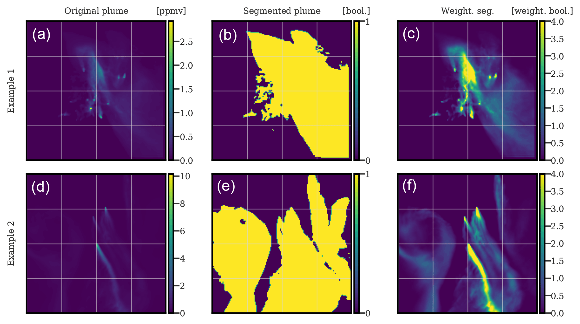
Figure 4Examples of XCO2 plumes (a, d), corresponding Boolean maps representing plume positions (b, e), and weighted Boolean maps representing the plume positions (c, f). The weighting is calculated according to Eq. (3).
These Boolean targets are visually far from representative of the plumes; the bulk of the signal, the mass of CO2, is contained in a much narrower area. In practice, this choice hinders the convergence and deeply degrades the performance of the CNN, since many pixels with low plume concentration are difficult to detect. A threshold could be used to generate more representative Boolean targets, but due to the diversity of plume types, no universal threshold exists.
To overcome this problem, the pixel loss is weighted by a function proportional to the plume concentration of the pixel. The weight function, depending on the plume concentration in the pixel, is linear and is defined by
where c≥0 is the plume concentration of the pixel, ymin=0.05 ppm. Furthermore, we choose to set ymax as the 99th percentile of the plume concentrations, instead of the maximum, to avoid outliers. With this weighting, the loss on a prediction field pi,j becomes
where ci,j is the true plume concentration at pixel (i,j), and yi,j is a Boolean indicating whether a pixel is part of the plume or not. After preliminary sensitivity experiments (not illustrated here), wmin and wmax are set as 0.01 and 4. With these values, the model response is weighted as follows:
-
It is heavily penalised if it makes an error in a pixel with a high plume concentration.
-
It is penalised very little (even insignificantly) if it makes an error in a pixel associated with a low plume concentration.
-
It is moderately penalised if it makes an error in a non-plume pixel.
The result of this weighting can be observed in the right column of Fig. 4 because each pixel is still a Boolean but weighted depending on the plume concentration of the pixel.
The new loss function is differentiable, which is a necessary condition for the application of the gradient descent backpropagation algorithm. Moreover, the weighting is carried out independently for each field and plume pair and not uniformly for the whole dataset. This latter choice would have penalised low-emission hotspots and favoured high-emission ones. This loss function is referred to as the weighted binary cross-entropy (WBCE) in the following.
In practice, during the training phase, the plumes undergo a two-step transformation process. First, they are transformed using the weight function described in Eq. (3). Subsequently, they undergo further transformation using the data augmentation techniques specified in Sect. 2.2. The resulting transformed plumes are subjected to the loss function defined in Eq. (4) during training.
3.3 U-Net model
The deep learning model chosen to address this image-to-image problem follows the U-Net architecture, a CNN encoder–decoder originally developed for biomedical image segmentation (Ronneberger et al., 2015) but later successively applied in many domains. This architecture is composed of (i) a downsampling or encoder phase, where the resolution of the input image decreases and the number of feature channels increases, and (ii) of an upsampling or decoder phase, where the resolution is increased to its original shape, while the number of feature channels decreases symmetrically to the downsampling phase. The encoder captures and learns aggregated information locally, progressing until it captures close to the entire image. The encoder works in the same way as, for example, a classification model and can be built with any conventional CNN classifier. The decoder use the encoded information to build the output. The particularity of the U-Net architecture is the use of skip connections, where encoded layers are directly carried to the decoder part. In other words, the decoder part collects the high-resolution features from the encoder part through concatenation to prevent any information loss.
Many encoder and decoder architectures can be used, and an example is illustrated in Fig. 5.
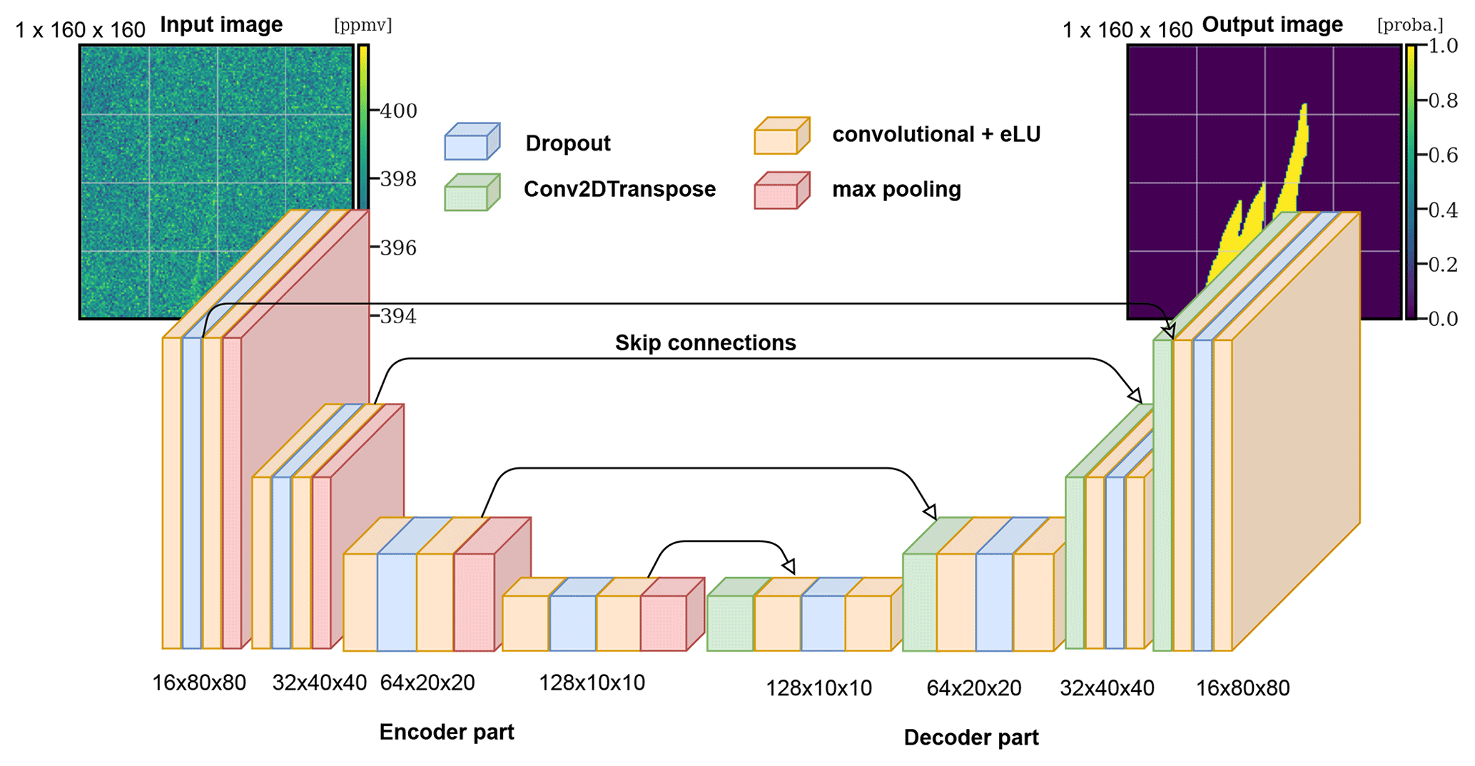
Figure 5The XCO2 field and plume pairs are fed into a U-Net algorithm that learns to distinguish the spatial features of the plume from the background.
Such a U-Net algorithm is built on top of convolutional layers that locally aggregate the information. Furthermore, the encoder uses max-pooling layers, which decrease the resolution of the image, while the decoder resorts to upsampling layers. Finally, dropout layers are used to reduce overfitting. However, in this paper, we use a generalised architecture (not shown for the sake of readability, since more than 270 layers and 5×10⁶ parameters are used). The encoder used is the EfficientNetB0 CNN architecture (Tan and Le, 2020), which is built with specific convolution layers (based on depth-wise convolutions) and a squeeze-and-excitation optimisation. Several encoders have been considered and tested, including ResNet (He et al., 2015), DenseNet (Huang et al., 2018), and self-made alternatives. The decoder phase is a repetition of the convolution and upsampling layers.
A dropout rate of 0.2 is used in the encoder part. The activation layers in the encoder part are swish functions (Ramachandran et al., 2017), whereas rectified linear activation functions (ReLUs) are chosen for the decoder part. The normal kernels are chosen to initialise the convolutional layers to avoid vanishing or exploding gradients during the first epochs. To obtain a probability map, the final output is activated by a sigmoid function. We use an initial learning rate of 10−3 with an Adam optimiser and a reduce-on-plateau strategy after considering different configurations. The batch size is set to 32 samples, and the number of epochs is set to 500, which ensures the convergence of learning. The final model weights are the best-performing weights on the validation dataset.
3.4 Training, validation, and test datasets
The complete dataset is divided into training, validation, and test subsets. Since a plume at a certain time strongly resembles the plume of the next hour, the validation and test sets consist of subsets of plumes on 2 consecutive days. For a given month, the test dataset always consists of the plumes of the 4th, 5th, 15th, and 16th days of the month. The training, validation, and test datasets are used to train the model, to tune its hyperparameter, and to test the optimal model, respectively.
The amounts of data for training, validation, and test differ for each test case. In the last case (extrapolation to Berlin), there are about 23 000 images in the training dataset, 4000 in the validation dataset, and 7000 in the test dataset. It is worth mentioning that data augmentation techniques enable us to use a significantly greater number of training images in practice.
The input XCO2 fields are standardised using the mean and variance over all pixels of all images of the training dataset. All the results in the following Sect. 4 were obtained on the test dataset, which was unobserved until the final evaluation. Furthermore, the results are obtained on a non-augmented test dataset, since the WBCE metrics of the model on augmented or non-augmented test datasets are similar, and we are primarily interested in segmenting non-augmented images.
To evaluate the performances of the CNN plume segmentation, two alternative segmentations to compare the performances to (hereafter called references) are described in Sect. 4.1. Then, the U-Net algorithm is trained and tested in two configurations.
In Sect. 4.2, the first configuration, we investigate the ability of the U-Net algorithm to generalise to new data from the same region. The U-Net algorithm is trained and tested on pairs of XCO2 and plume images in Grand Paris, IdF, Berlin, Lippendorf, and in plume clusters centred at Jänschwalde or Boxberg. Several training set-ups are considered, where the CNN is trained either on all available data or only on data from one location.
In Sect. 4.3, the second configuration, we investigate the ability of the U-Net algorithm to extrapolate on unseen data from another area. The U-Net algorithm is trained on pairs of XCO2 and plume images in Grand Paris, IdF, Jänschwalde, Lippendorf, and Boxberg and tested on Berlin images.
4.1 Alternative segmentations for comparison
4.1.1 Neutral reference
Two references are considered to assess the quality of the CNN segmentation through their WBCE scores. First, we use a constant probability map as a first reference, which is in practice equivalent to a prediction of non-segmentation of the plume. Since the WBCE metric only deals with probabilities (rather than Boolean values), this constant value is a probability and must be chosen. For each hotspot dataset, this probability is found to be the one minimising the WBCE over all images of that hotspot with a differential evolution algorithm (Virtanen et al., 2020; Storn and Price, 1997). In practice, for each hotspot, the calculated probability is close to 0.15–0.2. This first segmentation reference output is called the neutral reference in the following. Figure 6 shows the histograms of the WBCE computed on the plume cluster centred at Boxberg and the Berlin plume with respect to the neutral reference.
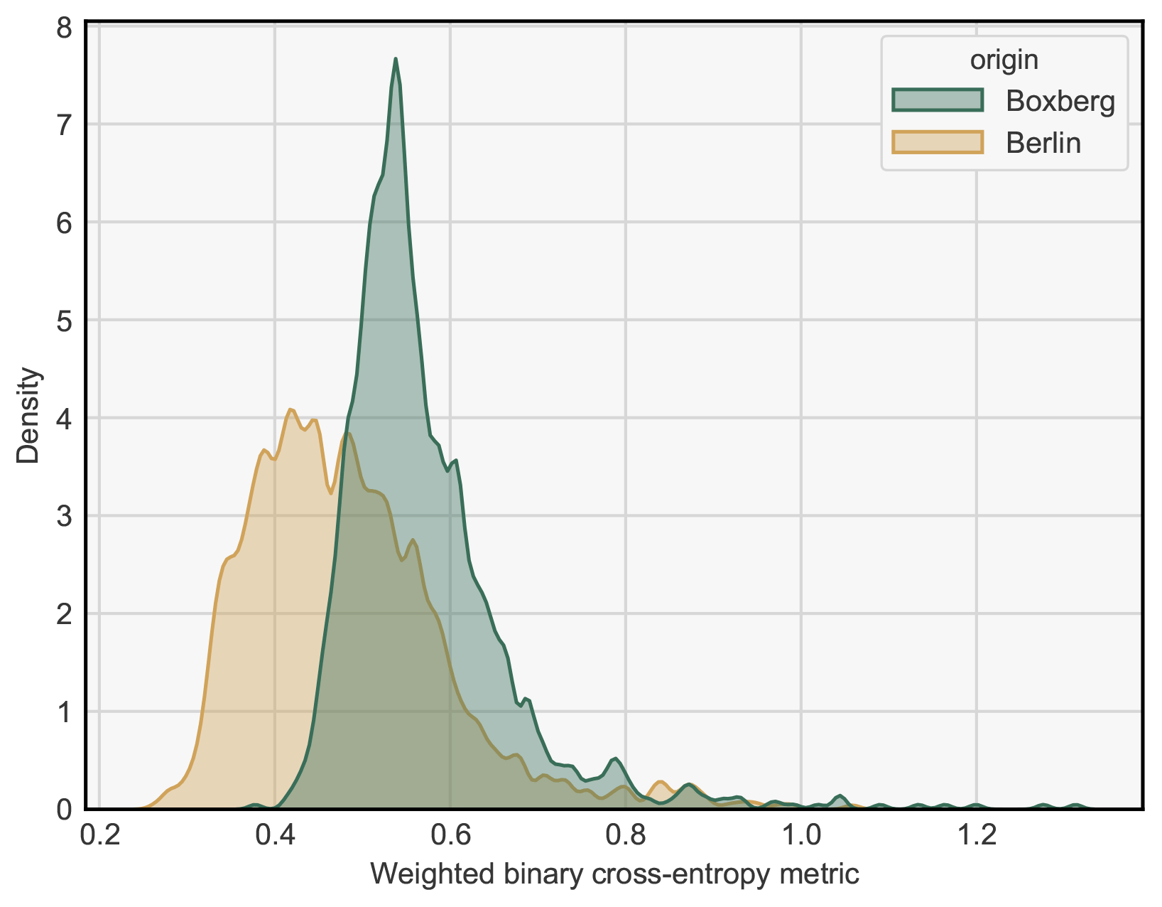
Figure 6Histograms of the WBCE scores over all images in Berlin and Boxberg obtained with the neutral reference.
Large variations can be observed because the neutral WBCE score for the Berlin images varies between 0.25 and 1. This means that the score associated with a segmentation is very dependent on the image considered; for one image, a score of 0.25 corresponds to a good segmentation, and for another image, such a score is equal to the neutral score and therefore equivalent to the absence of plume detection. Therefore, in the following, to make the segmentation scores more consistent over the samples, the WBCE of an image is systematically divided by its WBCE obtained with the neutral reference segmentation. This new metric is called the NWBCE (normalised weighted binary cross-entropy metric), and a score of 1 means that the resulting segmentation is no better than having no detection.
4.1.2 A segmentation technique based on thresholding: ddeq
The second reference to be compared with our segmentation method is the detection algorithm implemented in the Python package for data-driven emission quantification (ddeq; https://gitlab.com/empa503/remote-sensing/ddeq, last access: 10 July 2023)). This algorithm can be described as a thresholding method because it first detects the signal enhancements that are significant in relation to instrument noise and background variability and then identifies plumes as coherent structures (Kuhlmann et al., 2019a, 2021). Since the algorithm returns a Boolean map, the identified non-plume and plume pixels (0 and 1) are mapped to two values, which are defined independently for each hotspot. These two values are chosen so as to minimise the WBCE over all images from the hotspot. Figure 7 shows four applications of the ddeq algorithm to the CO2 images (two plume clusters centred in Boxberg and two in Berlin).
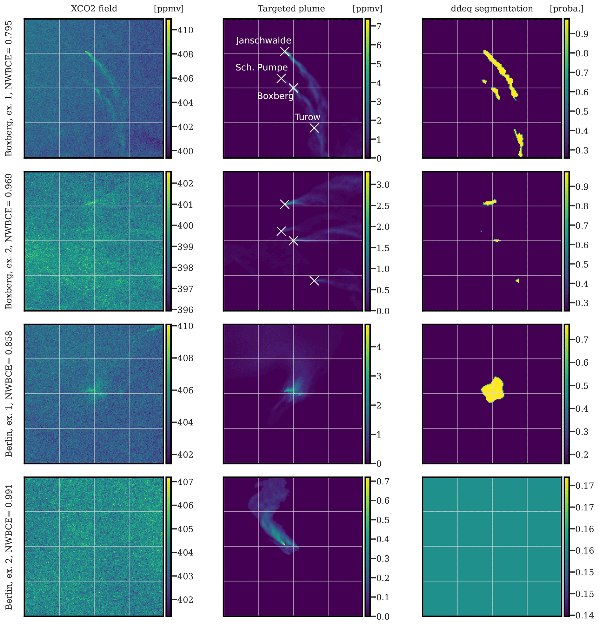
Figure 7Four examples of ddeq plume segmentation algorithm applications on simulated satellite images centred at Boxberg (first two rows) or Berlin (last two rows). The first column corresponds to XCO2 simulated satellite images in ppmv, the second column to the targeted plumes, and the third column to the predictions of the ddeq segmentation algorithm mapped to probability images. All times given to the left of the figures are in UTC.
The first plume cluster (centred in Boxberg) image (first row) obtains a much better NWBCE (0.79) than the second example (0.97) because the plume signal-to-background ratio is much higher. The same is true for the Berlin plume segmentations. Furthermore, due to the low SNR, no plume is detected on the fourth example, and a constant probability map is returned (which gives a score close to the neutral, and not 1, because the mapped probability is different). The thresholding method allows the segmentation of plumes, or portions of plumes, associated with signals above the background. But if no visible signal above the background is detected, then the plume is not identified.
4.2 Generalisation on new data from the same region
4.2.1 Choice of the training dataset
In this section, we investigate the performance of the U-Net algorithm when trained and tested on data from the same region. We consider two ways to train the model, namely to train to segment plumes on images of a given location, so that the U-Net algorithm can either exploit only the XCO2 field and plume pairs from that specific location, or the XCO2 field and plume pairs from all available locations. The two approaches yield different results, as summarised in Table 2.
Table 2NWBCE mean–median over the XCO2 field and plume pairs (i.e. overall model performance) of a certain region in two situations, where the U-Net algorithm is either trained on fields from the same region or on all available data. The lower the score, the better.
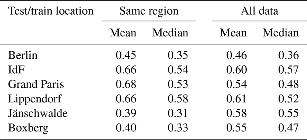
In the case of Berlin and IdF, the two training set-ups give approximately the same results for the mean and median. In the case of the Grand Paris and, to a lesser extent, Lippendorf, using additional training data improves the quality of the results. For the Paris fields, this might come from a lack of data (only 3 months). In contrast, in the Jänschwalde and Boxberg cases, using additional data degrades the results. This is most likely due to the fact that these two areas are characterised by multiple plumes (on the same image). In the following sections, we present the predictions for the best training configuration. In the case of Berlin, Grand Paris, IdF, and Lippendorf, the U-Net algorithm trained on all available data is used, and in the case of Jänschwalde and Boxberg, the U-Net algorithm trained with a restricted dataset is used.
4.2.2 Score histograms
Figure 8 presents the kernel density estimates of the NWBCE scores of the U-Net algorithm and ddeq segmentation methods, according to the origin of the XCO2 field and plume pair.
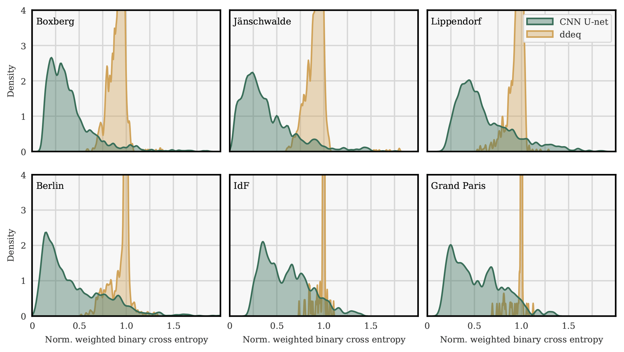
Figure 8Kernel densities of the histograms of the NWBCE scores of the U-Net algorithm and ddeq segmentation techniques over all images of the various geographical domains.
As a general rule, the lower the score, the better the segmentation. As shown in the following examples, scores between 0 and 0.5 usually correspond to very good to good segmentation and scores between 0.5 and 0.8 to 0.9 to non-perfect but usable segmentation. A score of 1 is neutral (neither worse nor better than predicting no plume), and a score above 1 corresponds to a worse segmentation than the neutral (i.e. a segmentation of the wrong part of the image). A number of applications with scores are presented in the following.
For all hotspots, our deep learning model consistently outperforms the ddeq segmentation method on the NWBCE metric. For example, the average NWBCE over all Berlin images is 1.0 for the neutral (by definition), 0.95 for the ddeq method, and 0.44 for the CNN segmentation. Over all Jänschwalde images, the average NWBCE is 0.90 for the ddeq method and 0.40 for the CNN method. Note, however, that the CNN is optimised on the NWBCE metric, whereas the ddeq segmentation method is not. The choice of a metric is to some extent arbitrary, and the difference between the two methods would change if another metric, and/or another definition of the plume, were chosen.
The best segmentation scores are obtained for Jänschwalde and Boxberg, which is consistent with the fact that these images contain several plumes of high intensity. The histogram of the Lippendorf NWBCE metric shows overall very good results but with a large variance and a significant part of the scores above 1. The distribution of the Berlin fields has a wider tail than that of the power plant fields; this can be explained by the shape of the city's plumes, which are generally more complex and therefore more difficult to segment than the straight power plant plumes. The poorer results over Grand Paris and IdF, on average, are due to the smaller number of available images and the low SNR of Grand Paris plumes. The small plumes specific to IdF (outside of Grand Paris) are almost never recovered, as shown in the IdF histogram, which is similar to the Grand Paris histogram but slightly shifted to the right.
4.2.3 Berlin region predictions
In Fig. 9, we present four typical Berlin plume segmentations with the U-Net algorithm. The XCO2 images (left column) are fed into the CNN, which yields the segmentation probability maps (right column) of the XCO2 plumes. For the classical binary cross-entropy metric, a pixel with a probability equal to 0.5 means no information on the class of the pixel (plume or non-plume). We assume that this can be extended to the WBCE metric because all pixels with a probability greater than 0.5 can be considered to be part of a plume, while pixels below 0.5 can be considered to be pixels that are not part of a plume. Consequently, a divergent (at 0.5) colour map is used to represent the CNN model predictions. The middle images are the weighted Boolean map transformations (according to Eq. 3) of the actual plumes for comparison. The four images in order are illustrative of the four quartiles in terms of their performances, respectively (according to their NWBCE score).
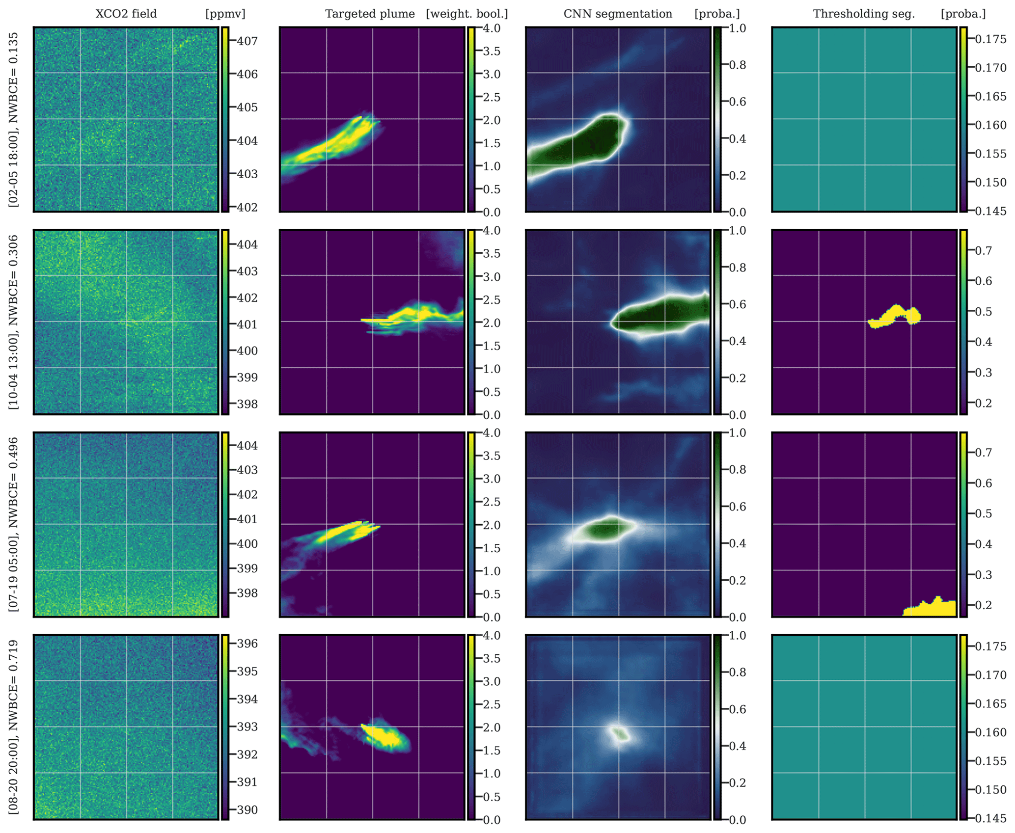
Figure 9Examples of the application of U-Net algorithm to images in the Berlin region. The first, second, and third columns correspond to XCO2 images of Berlin, weighted Boolean plumes, and CNN predictions as probability maps, respectively. The fourth column shows the application of the detection algorithm implemented in the Python package ddeq. The first, second, third, and fourth rows are representative of the first, second, third, and fourth quartiles of the NWBCE scores, respectively. All times given to the left of the figures are in UTC.
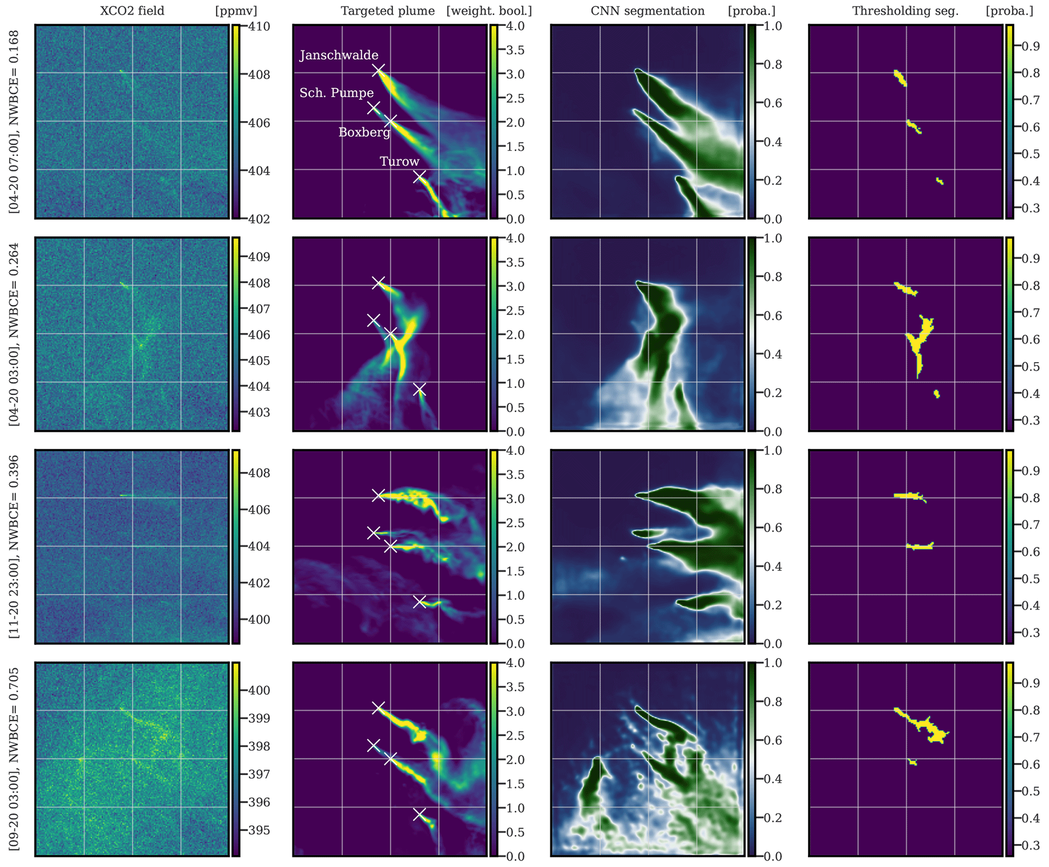
Figure 10Examples of the application of U-Net algorithm on images centred at Boxberg. Sources are shown from bottom to top in each image, with Turow, Boxberg, Schwarze Pumpe, and Jänschwalde. The first, second, and third columns correspond to the XCO2 images, weighted Boolean plumes, and CNN predictions as probability maps, respectively. The fourth column shows the application of the detection algorithm implemented in the Python package ddeq. The first, second, third, and fourth rows are representative of the first, second, third, and fourth quartiles of the NWBCE scores, respectively. All times given to the left of the figures are in UTC.
The first and second rows show a very accurate segmentation, as the model predicts the correct direction, shape, and thickness of the plume. The third plume is rather well recovered but with some inaccuracies; in particular, the tail of the plume is reconstructed with less accuracy, which was expected since the concentrations on the tail reach very low values. Moreover, the core of the plume is segmented with less confidence, and the probabilities of the plume pixels are close to 0.8. In general, the prediction confidence is positively correlated with the NWBCE score. Similarly, the uncertainty, represented by the number of pixels close to 0.5, and the NWBCE score are inversely correlated. To a certain extent, this is true for all hotspots and is a measure of model uncertainty. It can also be used in evaluations without access to the truth to quantify how certain the predictions are. Confirming this correlation, the fourth row shows a very uncertain prediction that still correctly finds the direction and core of the plume. For all images, the position of the plume origin is always accurate. This is not trivial because, in the training set, horizontal and vertical shifts are used, which means that the plume origin is not known in advance by the model. We note that the plume is often masked by background variability and instrument noise, which does not prevent its detection by the CNN.
4.2.4 Plume cluster centred in Boxberg predictions
In Fig. 10, the segmentation of four images centred at Boxberg power plant is shown. Sources are shown from the bottom to the top of the images, featuring Turow, Boxberg, Schwarze Pumpe, and Jänschwalde. The four images in order are representative of the four quartiles of their NWBCE score, respectively.
All first three segmentations are very accurate, and the origins, thicknesses, and directions of the plumes are accurately reconstructed. Some failures seen in are the mixing of the two plumes in the centre of the first image, the no detection of the Schwarze Pumpe plume in the second image, or the wrong evaluation of the direction of the Turow plume in the third image. The fourth segmentation's high NWBCE is mainly due to the addition by the model, with a high probability of a ghost plume to the left of the image, and a clear enhancement on the XCO2 field at the same location explains the U-Net error. The absence of power plants or major cities in the area raises questions about the origin of this enhancement.
4.2.5 Lippendorf predictions
In Fig. 11, we show the segmentation of four images centred at the Lippendorf power plant. The four images from top to bottom are illustrative of the four quartiles of their NWBCE score.
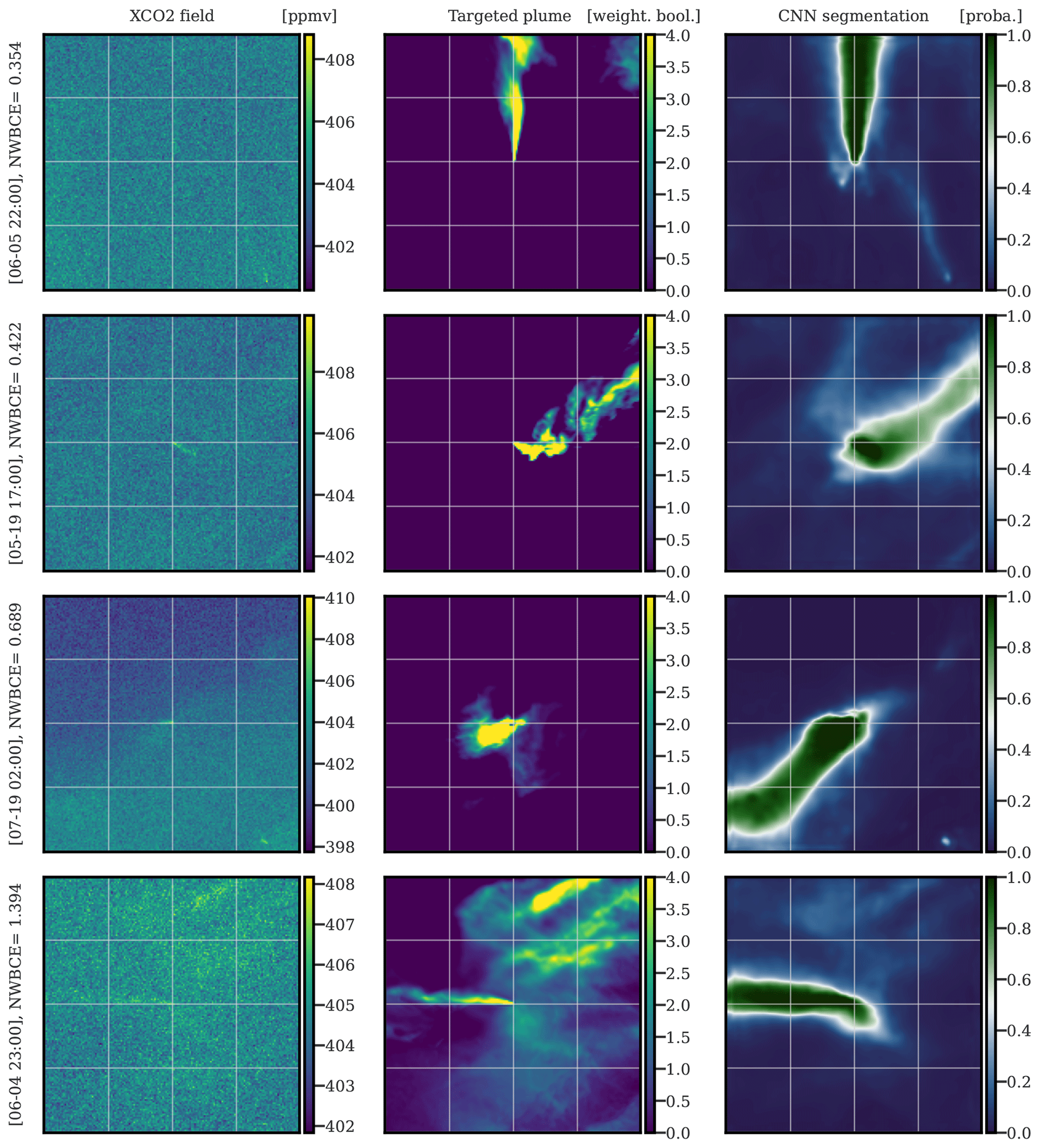
Figure 11Examples of the application of U-Net algorithm on images centred at Lippendorf. The first, second, and third columns correspond to XCO2 images, weighted Boolean plumes, and CNN predictions as probability maps, respectively. The first, second, third, and fourth rows are in the first, second, third, and fourth quartiles of the NWBCE scores, respectively. All times given to the left of the figures are in UTC.
The first two XCO2 images are well segmented, and the origins, thicknesses, and directions of the plumes are retrieved by the CNN model. The third row shows a strange behaviour of the plume which is not well anticipated by the model (i.e. the plume returns itself). The fourth line shows a very poor recovery, with a score of less than 1. The Lippendorf plume is in fact well segmented, but the residuals of other plumes are not, resulting in a significant error. This problem is at the origin of a large part of the errors in the Lippendorf images and could be solved by using a better loss/metric that would take into account the position of the source. A complementary study on the overall performance of the model can be found in the Supplement.
4.2.6 Paris predictions
In Fig. 12, we present four typical IdF plume segmentations, with or without the IdF specific plumes, using the U-Net algorithm. The four images in order are representative of the four quartiles of their NWBCE score, respectively.
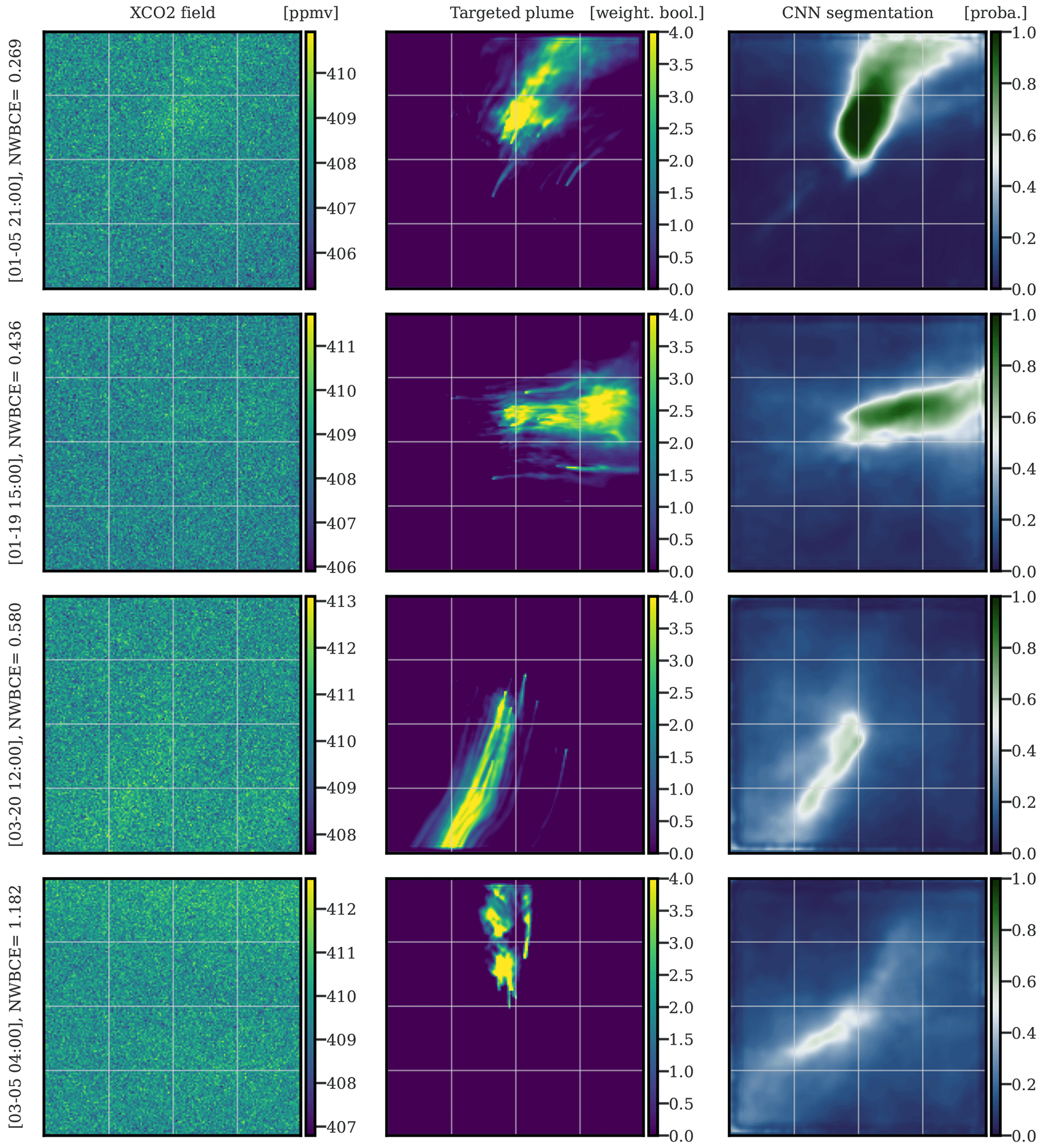
Figure 12Examples of the application of the U-Net algorithm on images of IdF. The first, second, and third columns correspond to XCO2 images of IdF, weighted Boolean plumes, and CNN predictions as probability maps, respectively. The first, second, third, and fourth rows are representative of the first, second, third, and fourth quartiles of the NWBCE scores, respectively. All times given to the left of the figures are in UTC.
The first three images show segmentations that reconstruct the direction and origin of the plume. However, the thickness is less and less well defined as the NWBCE increases. The other potential plumes outside Paris are systematically missed by the model because of their concentration being too low. Moreover, as the NWBCE increases, the pixel–plume predictions are closer and closer to 0.5, showing the hesitations of the model. Finally, the plume in the last image is completely missed, and the model makes no predictions above 0.55, expressing its inability to find the plume.
4.3 Extrapolation on unseen data from another region
In this section, we investigate the performance of the U-Net algorithm when trained and tested on data from different regions. This task is more difficult than generalising on plumes from the same region, where the training and test sets have more similarities due to the local climatology in terms of meteorology and pollution. To study the potential for extrapolation, the U-Net model is trained on the Paris, Jänschwalde, Boxberg, and Lippendorf fields and tested on the Berlin fields. Berlin is chosen because cities are a particularly complicated case, as their signal is lower and because, in this way, we can rely on a large set of images to validate and test the CNN model.
Figure 13 shows the histograms of the NWBCE scores for all Berlin test images, depending on the method used (left), and with the CNN method, in the case of the geographical extrapolation of all NWBCE scores for several ranges of the Berlin emissions rate at the time of the image (right).
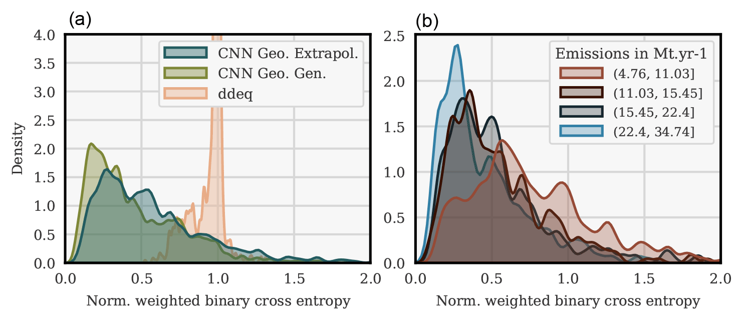
Figure 13Histograms of the NWBCE image scores over all test images of Berlin. Plumes/segmentations are classified depending on the method used (a). In the geographical extrapolation case, the CNN segmentation outputs are classified into four equivalent clusters, according to the corresponding emissions (b).
The mean NWBCE score of all prediction–truth pairs is 0.57, and the median is 0.49, which is higher in both cases compared to when the model is trained on Berlin images only (see Sect. 4.2) but still very satisfying; the model extrapolates well and outperforms the ddeq segmentations according to the NWBCE metric. In addition, the main divergence between the generalisation and extrapolation histograms is a shift to the right of the part of the histogram between the scores of 0 and 0.75. It is explained later in this section that segmentations with an NWBCE below 0.75 are generally good enough for inversion. In other words, the switch from generalisation to extrapolation mainly degrades highly accurate segmentations to “only” accurate segmentations.
The plumes that we assess are the consequence of a variety of emissions levels. For example, Berlin emissions range from approximately 4 to 35 Mt yr−1. In the right histogram, it can be observed that the results, quite naturally, deteriorate in the case of low-emission plumes. For high-emission plumes, the density peaks at 0.25, whereas it peaks at 0.5 in the case of low-emission plumes. The variance in the NWBCE metric density for the low-emission plumes is also significantly higher.
In Fig. 14, we present four typical Berlin plume segmentations with the U-Net algorithm. The four images from top to bottom are illustrative of the four quartiles, respectively (according to their NWBCE score).
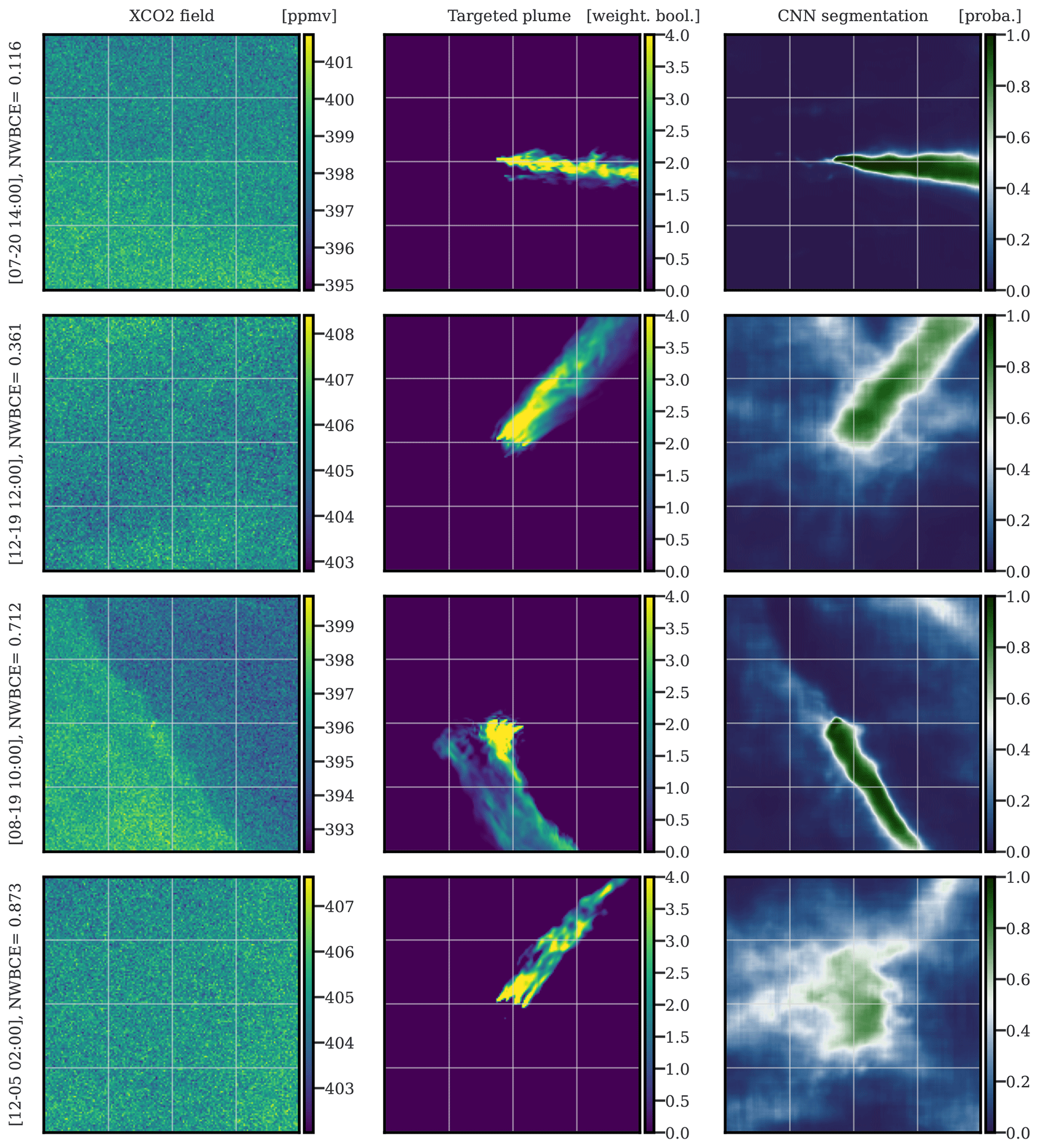
Figure 14Examples of the application of the U-Net algorithm on images of Berlin. The first, second, and third columns correspond to XCO2 images of Berlin, weighted Boolean plumes, and CNN predictions as probability maps, respectively. The first, second, third, and fourth rows are representative of the first, second, third, and fourth quartiles, respectively. All times given to the left of the figures are in UTC.
The first three images show segmentations that recover the direction and origin of the plume. The thickness of the plume is also well reconstructed in the first two examples, but part of the plume is missed in the third example, which gives the largest fraction of the error; this miss is probably due to a gradient in the background field. The second and third examples also show a significant number of pixels at values around 0.5, expressing the uncertainty in the model. In these examples, the plume is masked by background variability and instrument noise yet is still detected by the CNN. For the fourth example, the deep learning model fails to detect the plume and yet diagnoses higher uncertainty. Further analysis shows that most of the last quartile's results are difficult to use for inversion because they partially or completely miss the plume or express too much uncertainty.
The future availability of satellite images of CO2 columns, such as the Copernicus CO2 Monitoring (CO2M) mission, opens up new possibilities for the assessment of local CO2 emissions. Emissions can be assessed from CO2 plumes of hotspots in the satellite images (Nassar et al., 2017, 2022). This data-driven assessment needs to detect plumes from satellite images, which is difficult for the thresholding method due to the low SNR of the plume. Deep learning and convolutional neural network (CNN) techniques could provide more accurate plume detection because of their ability to learn and capture plume-specific spatial patterns, which do not necessarily depend on a significant concentration enhancement.
In this paper, we evaluate the ability of CNNs to accurately detect the mask of a plume in an XCO2 satellite image using simulated CO2 fields. Each synthetic XCO2 image is the sum of the anthropogenic plume of a major hotspot (a city or a power plant), background from other biogenic and anthropogenic fluxes, and a random Gaussian noise to simulate the satellite instrumental errors.
Our plume detection model is based on a CNN encoder–decoder, the U-Net algorithm, with an EfficientNetB0 backbone. It is an image-to-image model, which transforms the full XCO2 field into a map showing the positions of the anthropogenic emission plumes. For training, we develop a novel loss function that penalises the errors made on pixels associated with high plume concentrations more and thus yields a more accurate definition of a plume than a simple threshold value. This CNN is trained and tested in two contexts. First, the capacity of the model to generalise on unseen data from the same region is evaluated. The U-Net algorithm shows very good performance, as most plumes are precisely segmented, and the origin, thickness, and shape of the plume are often accurately retrieved. Second, we evaluate the ability of the model to extrapolate to unobserved data from another region. Specifically, the model is trained with simulated fields of Paris and power plants and tested with fields in the Berlin area. The segmentations are slightly less accurate than in the first context but are nevertheless very satisfactory; about half of the Berlin plumes are accurately segmented, with the plume shape, thickness, direction, and origin being recovered, and 75 % of the segmentations are accurate enough to be used for inversion.
The observed good performance of the U-Net architecture is due to the ability of the convolution layers to capture detailed spatial patterns corresponding to plumes, even when the concentrations of these plumes are partially covered by high satellite noise or background variability. It allows the model to outperform the segmentations done by the thresholding technique, according to the concentration-weighted metric, whether the model trained on some data is tested on data from the same region or not. The U-Net algorithm is effective over a wide variety of plumes (cities, power plants, diverse regions, and several levels of hotspot emissions). Its training time is less than 1 d, while once the model has been trained, the evaluation of a new image is less than a second. However, although the model performs better when trained and tested on data from the same region, it would be too expensive to generate simulations on all the cities and power plants whose plumes we wish to segment. Therefore, we believe that the goal is the development of a universal CNN, which is trained only on a limited sample of cities and power plants and highly efficient on all of them. The model in this paper, trained on Paris and power plant data and tested on Berlin, already shows accurate and very satisfactory segmentations of the Berlin plumes, but the results need to be confirmed on multiple cases.
It is very likely that many other techniques could be applied to improve these segmentations, which could be based on the following:
-
more advanced and powerful NN architectures, such as transformers, or on CNN networks with more parameters; and
-
an improvement of the distribution of the data by increasing the number of images used or by using more carefully chosen augmentation techniques.
For all of these reasons, CNN methods appear to be very suitable for CO2 plume segmentation problems on satellite data. However, the model was evaluated on simulated data, which does not take into account all the problems of plume detectability presented by real satellite images (in particular clouds and patterns of systematic errors) due to surface reflectance and the aerosol dependency of the retrievals. Consequently, the method needs to be extended and validated on full OSSEs, where fields with clouds and satellite swaths are taken into account, and afterwards on real satellite data.
Finally, as the CO2 emission rate is proportional to the mass of the corresponding plume, accurate plume segmentation should lead to an accurate emission estimate. The reliability and accuracy of the CNN model segmentations suggest that a well-trained CNN fed by these segmented plumes could be a very efficient hotspot estimator.
The datasets used in this paper are available from a compliant repository at https://doi.org/10.5281/zenodo.4048228 (Kuhlmann et al., 2020b) for the SMARTCARB data (for Berlin and power plants based in Germany). The code is available from a compliant repository at https://doi.org/10.5281/zenodo.7371413 (Dumont Le Brazidec, 2022).
The supplement related to this article is available online at: https://doi.org/10.5194/gmd-16-3997-2023-supplement.
JDLB: conceptualisation, methodology, software, investigation, formal analysis, visualisation, resources, project administration, and writing the original draft. PV: investigation, formal analysis, and paper review. AF: conceptualisation, methodology, project administration, and paper review. MB: conceptualisation, methodology, project administration, funding acquisition, and paper review. JL, GB, GK, and AD: paper review. JL, GB, GK, AD and TL: resources.
The authors declare that they have no conflict of interest.
Publisher's note: Copernicus Publications remains neutral with regard to jurisdictional claims in published maps and institutional affiliations.
This project has been funded by the European Union's Horizon 2020 research and innovation programme (grant no. 958927; prototype system for a Copernicus CO2 service). CEREA is a member of the Institute Pierre-Simon Laplace (IPSL). The authors would like to thank Hugo Denier van der Gon for the TNO inventory and Élise Potier for her contribution to the development of the Paris dataset. The authors would like to thank the reviewers for their meaningful contributions.
This research has been supported by the Horizon 2020 (grant no. 958927).
This paper was edited by Jinkyu Hong and reviewed by Ray Nassar and one anonymous referee.
Agustí-Panareda, A., Massart, S., Chevallier, F., Boussetta, S., Balsamo, G., Beljaars, A., Ciais, P., Deutscher, N. M., Engelen, R., Jones, L., Kivi, R., Paris, J.-D., Peuch, V.-H., Sherlock, V., Vermeulen, A. T., Wennberg, P. O., and Wunch, D.: Forecasting global atmospheric CO2, Atmos. Chem. Phys., 14, 11959–11983, https://doi.org/10.5194/acp-14-11959-2014, 2014. a
Brunner, D., Kuhlmann, G., Marshall, J., Clément, V., Fuhrer, O., Broquet, G., Löscher, A., and Meijer, Y.: Accounting for the vertical distribution of emissions in atmospheric CO2 simulations, Atmos. Chem. Phys., 19, 4541–4559, https://doi.org/10.5194/acp-19-4541-2019, 2019. a
Butz, A., Scheidweiler, L., Baumgartner, A., Feist, D. G., Gottschaldt, K.-D., Jöckel, P., Kern, B., Köhler, C., Krutz, D., Lichtenberg, G., Marshall, J., Paproth, C., Slijkhuis, S., Sebastian, I., Strandgren, J., Wilzewski, J. S., and Roiger, A.: CO2Image: a next generation imaging spectrometer for CO2 point source quantification, EGU General Assembly 2022, Vienna, Austria, 23–27 May 2022, EGU22-6324, https://doi.org/10.5194/egusphere-egu22-6324, 2022. a
Chevallier, F.: Validation report for the inverted CO2 fluxes, v18r1 – version 1.0, Copernicus Atmosphere Monitoring Service, p. 20, https://atmosphere.copernicus.eu/sites/default/files/2019-01/CAMS73_2018SC1_D73.1.4.1-2017-v0_201812_v1_final.pdf (last access: 10 July 2023), 2018. a
Chollet, F.: Deep Learning with Python, 1st edn., Manning Publications, 384 pp., ISBN 978-1617294433, 2017. a, b, c
Crisp, D., Pollock, H. R., Rosenberg, R., Chapsky, L., Lee, R. A. M., Oyafuso, F. A., Frankenberg, C., O'Dell, C. W., Bruegge, C. J., Doran, G. B., Eldering, A., Fisher, B. M., Fu, D., Gunson, M. R., Mandrake, L., Osterman, G. B., Schwandner, F. M., Sun, K., Taylor, T. E., Wennberg, P. O., and Wunch, D.: The on-orbit performance of the Orbiting Carbon Observatory-2 (OCO-2) instrument and its radiometrically calibrated products, Atmos. Meas. Tech., 10, 59–81, https://doi.org/10.5194/amt-10-59-2017, 2017. a
Denier van der Gon, H., Dellaert, S., Super, I., Kuenen, J., and Visschedijk, A.: VERIFY: Observation-based system for monitoring and verification of greenhouse gases, https://cordis.europa.eu/project/id/776810/reporting (last access: 10 July 2023), 2021. a
Dumont Le Brazidec, J.: cerea-daml/co2-images-seg: XCO2 simulated satellite image segmentation paper (co2-seg-paper-sub), Zenodo [code], https://doi.org/10.5281/zenodo.7371413, 2022. a
Finch, D. P., Palmer, P. I., and Zhang, T.: Automated detection of atmospheric NO2 plumes from satellite data: a tool to help infer anthropogenic combustion emissions, Atmos. Meas. Tech., 15, 721–733, https://doi.org/10.5194/amt-15-721-2022, 2022. a
Grell, G. A., Peckham, S. E., Schmitz, R., McKeen, S. A., Frost, G., Skamarock, W. C., and Eder, B.: Fully coupled “online” chemistry within the WRF model, Atmos. Environ., 39, 6957–6975, https://doi.org/10.1016/j.atmosenv.2005.04.027, 2005. a
Hakkarainen, J., Ialongo, I., Koene, E., Szelag, M., Tamminen, J., Kuhlmann, G., and Brunner, D.: Analyzing Local Carbon Dioxide and Nitrogen Oxide Emissions From Space Using the Divergence Method: An Application to the Synthetic SMARTCARB Dataset, Front. Remote Sens., 3, https://doi.org/10.3389/frsen.2022.878731, 2022. a
He, K., Zhang, X., Ren, S., and Sun, J.: Deep Residual Learning for Image Recognition, ArXiv, https://doi.org/10.48550/arXiv.1512.03385, 2015. a
Hersbach, H., Bell, B., Berrisford, P., Hirahara, S., Horányi, A., Muñoz‐Sabater, J., Nicolas, J., Peubey, C., Radu, R., Schepers, D., Simmons, A., Soci, C., Abdalla, S., Abellan, X., Balsamo, G., Bechtold, P., Biavati, G., Bidlot, J., Bonavita, M., Chiara, G. D., Dahlgren, P., Dee, D., Diamantakis, M., Dragani, R., Flemming, J., Forbes, R., Fuentes, M., Geer, A., Haimberger, L., Healy, S., Hogan, R. J., Hólm, E., Janisková, M., Keeley, S., Laloyaux, P., Lopez, P., Lupu, C., Radnoti, G., Rosnay, P. d., Rozum, I., Vamborg, F., Villaume, S., and Thépaut, J.-N.: The ERA5 global reanalysis, Q. J. Roy. Meteorol. Soc., 146, 1999–2049, https://doi.org/10.1002/qj.3803, 2020. a
Huang, G., Liu, Z., van der Maaten, L., and Weinberger, K. Q.: Densely Connected Convolutional Networks, ArXiv, arXiv:1608.06993 [cs], https://doi.org/10.48550/arXiv.1608.06993, 2018. a
Jadon, S.: A survey of loss functions for semantic segmentation, 2020 IEEE Conference on Computational Intelligence in Bioinformatics and Computational Biology (CIBCB), Via del Mar, Chile, 2020, 1–7, https://doi.org/10.1109/CIBCB48159.2020.9277638, 2020. a
Janssens-Maenhout, G., Pinty, B., Dowell, M., Zunker, H., Andersson, E., Balsamo, G., Bézy, J.-L., Brunhes, T., Bösch, H., Bojkov, B., Brunner, D., Buchwitz, M., Crisp, D., Ciais, P., Counet, P., Dee, D., Gon, H. D. V. D., Dolman, H., Drinkwater, M. R., Dubovik, O., Engelen, R., Fehr, T., Fernandez, V., Heimann, M., Holmlund, K., Houweling, S., Husband, R., Juvyns, O., Kentarchos, A., Landgraf, J., Lang, R., Löscher, A., Marshall, J., Meijer, Y., Nakajima, M., Palmer, P. I., Peylin, P., Rayner, P., Scholze, M., Sierk, B., Tamminen, J., and Veefkind, P.: Toward an Operational Anthropogenic CO2 Emissions Monitoring and Verification Support Capacity, B. Am. Meteorol. Soc., 101, E1439–E1451, https://doi.org/10.1175/BAMS-D-19-0017.1, 2020. a
Kuenen, J. J. P., Visschedijk, A. J. H., Jozwicka, M., and Denier van der Gon, H. A. C.: TNO-MACC_II emission inventory; a multi-year (2003–2009) consistent high-resolution European emission inventory for air quality modelling, Atmos. Chem. Phys., 14, 10963–10976, https://doi.org/10.5194/acp-14-10963-2014, 2014. a
Kuhlmann, G., Broquet, G., Marshall, J., Clément, V., Löscher, A., Meijer, Y., and Brunner, D.: Detectability of CO2 emission plumes of cities and power plants with the Copernicus Anthropogenic CO2 Monitoring (CO2M) mission, Atmos. Meas. Tech., 12, 6695–6719, https://doi.org/10.5194/amt-12-6695-2019, 2019a. a, b, c, d, e, f
Kuhlmann, G., Clément, V., Marshall, J., Fuhrer, O., Broquet, G., Schnadt-Poberaj, C., Löscher, A., Meijer, Y., and Brunner, D.: SMARTCARB – Use of satellite measurements of auxiliary reactive trace gases for fossil fuel carbon dioxide emission estimation, Tech. rep., Zenodo [data set], https://doi.org/10.5281/zenodo.4034266, 2019b. a, b
Kuhlmann, G., Brunner, D., Broquet, G., and Meijer, Y.: Quantifying CO2 emissions of a city with the Copernicus Anthropogenic CO2 Monitoring satellite mission, Atmos. Meas. Tech., 13, 6733–6754, https://doi.org/10.5194/amt-13-6733-2020, 2020a. a
Kuhlmann, G., Clément, V., Marshall, J., Fuhrer, O., Broquet, G., Schnadt-Poberaj, C., Löscher, A., Meijer, Y., and Brunner, D.: Synthetic XCO2, CO and NO2 observations for the CO2M and Sentinel-5 satellites, Zenodo [data set], https://doi.org/10.5281/zenodo.4048228, 2020b. a, b
Kuhlmann, G., Henne, S., Meijer, Y., and Brunner, D.: Quantifying CO2 Emissions of Power Plants With CO2 and NO2 Imaging Satellites, Front. Remote Sens., 2, https://doi.org/10.3389/frsen.2021.689838, 2021. a, b, c
Lauvaux, T., Giron, C., Mazzolini, M., d’Aspremont, A., Duren, R., Cusworth, D., Shindell, D., and Ciais, P.: Global assessment of oil and gas methane ultra-emitters, Science, 375, 557–561, https://doi.org/10.1126/science.abj4351, 2022. a
Lian, J., Bréon, F.-M., Broquet, G., Lauvaux, T., Zheng, B., Ramonet, M., Xueref-Remy, I., Kotthaus, S., Haeffelin, M., and Ciais, P.: Sensitivity to the sources of uncertainties in the modeling of atmospheric CO2 concentration within and in the vicinity of Paris, Atmos. Chem. Phys., 21, 10707–10726, https://doi.org/10.5194/acp-21-10707-2021, 2021. a
Mahadevan, P., Wofsy, S., Matross, D., Xiao, X., Dunn, A., Lin, J., Gerbig, C., Munger, J., Chow, V., and Gottlieb, E.: A Satellite-based Biosphere Parameterization for Net Ecosystem CO2 Exchange: Vegetation Photosynthesis and Respiration Model (VPRM), Glob. Biogeochem. Cycles., 22, GB2005, https://doi.org/10.1029/2006GB002735, 2008. a, b
Meijer, Y.: Copernicus CO2 Monitoring Mission Requirements Document, Earth and Mission Science Division, 84, https://esamultimedia.esa.int/docs/EarthObservation/CO2M_MRD_v3.0_20201001_Issued.pdf (last access: 10 July 2023), 2020. a
Nassar, R., Hill, T. G., McLinden, C. A., Wunch, D., Jones, D. B. A., and Crisp, D.: Quantifying CO2 Emissions From Individual Power Plants From Space, Geophys. Res. Lett., 44, 10045–10053, https://doi.org/10.1002/2017GL074702, 2017. a
Nassar, R., Moeini, O., Mastrogiacomo, J.-P., O'Dell, C. W., Nelson, R. R., Kiel, M., Chatterjee, A., Eldering, A., and Crisp, D.: Tracking CO2 emission reductions from space: A case study at Europe's largest fossil fuel power plant, Front. Remote Sens., 3, https://doi.org/10.3389/frsen.2022.1028240, 2022. a
Ramachandran, P., Zoph, B., and Le, Q. V.: Searching for Activation Functions, ArXiv, https://doi.org/10.48550/arXiv.1710.05941, 2017. a
Reuter, M., Buchwitz, M., Schneising, O., Krautwurst, S., O'Dell, C. W., Richter, A., Bovensmann, H., and Burrows, J. P.: Towards monitoring localized CO2 emissions from space: co-located regional CO2 and NO2 enhancements observed by the OCO-2 and S5P satellites, Atmos. Chem. Phys., 19, 9371–9383, https://doi.org/10.5194/acp-19-9371-2019, 2019. a
Ronneberger, O., Fischer, P., and Brox, T.: U-Net: Convolutional Networks for Biomedical Image Segmentation, arXiv:1505.04597 [cs], http://arxiv.org/abs/1505.04597, 2015. a
Storn, R. and Price, K.: Differential Evolution – A Simple and Efficient Heuristic for global Optimization over Continuous Spaces, J. Glob. Optim., 11, 341–359, https://doi.org/10.1023/A:1008202821328, 1997. a
Tan, M. and Le, Q. V.: EfficientNet: Rethinking Model Scaling for Convolutional Neural Networks, arXiv:1905.11946 [cs, stat], http://arxiv.org/abs/1905.11946, 2020. a
UNFCCC: Paris Agreement, {FCCC/CP/2015/L.9/Rev1}, http://unfccc.int/resource/docs/2015/cop21/eng/l09r01.pdf (last access: 10 July 2023), 2015. a
Virtanen, P., Gommers, R., Oliphant, T. E., Haberland, M., Reddy, T., Cournapeau, D., Burovski, E., Peterson, P., Weckesser, W., Bright, J., van der Walt, S. J., Brett, M., Wilson, J., Millman, K. J., Mayorov, N., Nelson, A. R. J., Jones, E., Kern, R., Larson, E., Carey, C. J., Polat, I., Feng, Y., Moore, E. W., VanderPlas, J., Laxalde, D., Perktold, J., Cimrman, R., Henriksen, I., Quintero, E. A., Harris, C. R., Archibald, A. M., Ribeiro, A. H., Pedregosa, F., van Mulbregt, P., SciPy 1.0 Contributors, Vijaykumar, A., Bardelli, A. P., Rothberg, A., Hilboll, A., Kloeckner, A., Scopatz, A., Lee, A., Rokem, A., Woods, C. N., Fulton, C., Masson, C., Häggström, C., Fitzgerald, C., Nicholson, D. A., Hagen, D. R., Pasechnik, D. V., Olivetti, E., Martin, E., Wieser, E., Silva, F., Lenders, F., Wilhelm, F., Young, G., Price, G. A., Ingold, G.-L., Allen, G. E., Lee, G. R., Audren, H., Probst, I., Dietrich, J. P., Silterra, J., Webber, J. T., Slavič, J., Nothman, J., Buchner, J., Kulick, J., Schönberger, J. L., de Miranda Cardoso, J. V., Reimer, J., Harrington, J., Rodríguez, J. L. C., Nunez-Iglesias, J., Kuczynski, J., Tritz, K., Thoma, M., Newville, M., Kümmerer, M., Bolingbroke, M., Tartre, M., Pak, M., Smith, N. J., Nowaczyk, N., Shebanov, N., Pavlyk, O., Brodtkorb, P. A., Lee, P., McGibbon, R. T., Feldbauer, R., Lewis, S., Tygier, S., Sievert, S., Vigna, S., Peterson, S., More, S., Pudlik, T., Oshima, T., Pingel, T. J., Robitaille, T. P., Spura, T., Jones, T. R., Cera, T., Leslie, T., Zito, T., Krauss, T., Upadhyay, U., Halchenko, Y. O., and Vázquez-Baeza, Y.: SciPy 1.0: fundamental algorithms for scientific computing in Python, Nat. Meth., 17, 261–272, https://doi.org/10.1038/s41592-019-0686-2, 2020. a, b
Zhang, A., Lipton, Z. C., Li, M., and Smola, A. J.: Dive into Deep Learning, ArXiv, https://doi.org/10.48550/arXiv.2106.11342, 2022. a, b