the Creative Commons Attribution 4.0 License.
the Creative Commons Attribution 4.0 License.
 | 13 Jan 2023
The tidal effects in the Finite-volumE Sea ice–Ocean Model (FESOM2.1): a comparison between parameterised tidal mixing and explicit tidal forcing
Dmitry Sidorenko
Patrick Scholz
Maik Thomas
Gerrit Lohmann
Tides are proved to have a significant effect on the ocean and climate. Previous modelling research either adds a tidal mixing parameterisation or an explicit tidal forcing to the ocean models. However, no research compares the two approaches in the same framework. Here we implement both schemes in a general ocean circulation model and assess both methods by comparing the results. The aspects for comparison involve hydrography, sea ice, meridional overturning circulation (MOC), vertical diffusivity, barotropic streamfunction and energy diagnostics. We conclude that although the mesh resolution is poor in resolving internal tides in most mid-latitude and shelf-break areas, explicit tidal forcing still shows stronger tidal mixing at the Kuril–Aleutian Ridge and the Indonesian Archipelago than the tidal mixing parameterisation. Beyond that, the explicit tidal forcing method leads to a stronger upper cell of the Atlantic MOC by enhancing the Pacific MOC and the Indonesian Throughflow. Meanwhile, the tidal mixing parameterisation leads to a stronger lower cell of the Atlantic MOC due to the tidal mixing in deep oceans. Both methods maintain the Antarctic Circumpolar Current at a higher level than the control run by increasing the meridional density gradient. We also show several phenomena that are not considered in the tidal mixing parameterisation, for example, the changing of energy budgets in the ocean system, the bottom drag induced mixing on the continental shelves and the sea ice transport by tidal motions. Due to the limit of computational capacity, an internal-tide-resolving simulation is not feasible for climate studies. However, a high-resolution short-term tidal simulation is still required to improve parameters and parameterisation schemes in climate studies.
- Article
(21117 KB) - Full-text XML
- BibTeX
- EndNote


Based on Sandström's theorem, the ocean is proved not to be a heat engine (e.g. Huang, 2009). This means the global thermohaline circulation (THC) is not driven by the heat difference between the Equator and the poles. A lot has been discussed on what is driving the global THC. Munk and Wunsch (1998) concluded that tides and winds maintain the global THC and ocean stratification. They also estimated the global mean vertical diffusivity (the same as diapycnal diffusivity in the whole context) to be 10−4 m2 s−1, which mismatches 10−5 m2 s−1 from observational results in most parts of the global ocean. Thus, some areas with large vertical diffusivities are expected to contribute to the global strength of upwelling. Observational results (Polzin et al., 1997; Ledwell et al., 2000) present large vertical diffusivities at near-bottom rough topographies in the Mid-Atlantic Ridge, which is believed to be generated by tide–topography interactions. These observational results indicate the significance of tide-induced mixing effects from a climatic point of view.
Tide-induced mixing has long been considered in modelling research. Plenty of research on tuning vertical diffusivity parameters has been conducted to reduce model biases. By testing different vertical diffusivity parameters in an ocean general circulation model (OGCM), Bryan (1987) found that ocean circulation is sensitive to vertical diffusivity. As vertical diffusivity increases, the thickness of ocean thermocline, the strength of meridional overturning circulation (MOC) and poleward heat transport increase. After the bottom-enhanced structure of vertical diffusivities is revealed from the observations (Polzin et al., 1997), the vertical diffusivity in ocean models is now considered a vertical profile and not a constant parameter anymore. Tsujino et al. (2000) discussed the influence of different vertical diffusivity profiles on the global ocean circulations, concluding that different profile shapes lead to different strengths of Pacific MOC (PMOC). However, most early research does not consider the horizontal inhomogeneity of tide-induced mixing in the global ocean. Since the formation of a tide-induced mixing parameterisation (St. Laurent et al., 2002; Simmons et al., 2004), a better treatment that considers both vertical variation and horizontal inhomogeneity of the vertical diffusivity is widely used in OGCMs. It should be noted here that the horizontal distribution of the enhanced vertical diffusivities is related to the baroclinic tide conversion rate, which is provided by an analytical or numerical tidal model (e.g. Jayne, 2009). Thus the horizontal distribution is closer to the real ocean. Following the Community Ocean Vertical Mixing (CVMIX; Griffies et al., 2015) library, hereinafter, we name this parameterisation CVMIX_TIDAL. In the following research, CVMIX_TIDAL, along with parameterisations with similar formulas (e.g. Friedrich et al., 2011; Tatebe et al., 2018), has been adopted in OGCMs to reveal the tidal effect on the ocean and climate. It has been proved that the consideration of tide-induced mixing may have an impact on aspects related to the global THC, for example, the Atlantic MOC (AMOC) (Simmons et al., 2004; Jayne, 2009), the strength and deepness of the Antarctic Circumpolar Current (ACC) (Saenko and Merryfield, 2005), the Southern Ocean sea ice and the Circumpolar Deep Water formation (Tatebe et al., 2018), the ventilation of the North Pacific Intermediate Water and the deep North Pacific circulation (Oka and Niwa, 2013), and the ocean biogeochemistry (Friedrich et al., 2011). Lee et al. (2006) also implemented bottom-enhanced vertical diffusivities in an OGCM. However, the main difference from above is that they enhanced vertical diffusivities on continental shelves, parameterising the tidal shear caused by the bottom drag in shallow areas. Their results show that the mixing caused by tidal shear on continental shelves improves the modelled hydrography in coastal areas and adjacent marginal seas.
Instead of adding parameterisation schemes to OGCMs, another way to consider the tidal effect is to add an explicit tidal forcing to the momentum equations. Global tides have been added to some OGCMs (e.g. Thomas et al., 2001; Shriver et al., 2012; Arbic et al., 2018; Logemann et al., 2021), but little research has been conducted from a climatic point of view. By comparing sensitivity runs with and without tidal motions in an OGCM, Schiller (2004) found that tidal motions can rectify Indonesian Archipelago hydrography and Indonesian Throughflow (ITF) transport. Similar work via a coupled climate model concludes that the simulation with tidal motions can improve the modelled North Atlantic Current and western European climate (Müller et al., 2010). Yu et al. (2016) also implemented a tidal module in an OGCM. But unlike the above research that concentrates on regional circulations, they discuss the influence on global hydrography and circulation. The main finding is that the tidal motions reduce the strength of wind-induced circulation and the upper cell of AMOC while slightly increasing the strength of the bottom cell of AMOC. In addition, a special kind of explicit forcing representing the tidal effect is the tidal residual circulation. By considering the tidal residual circulation an external forcing in an OGCM, Bessières et al. (2008) concluded that the ocean state is insensitive to the tidal residual circulation, which can be neglected in climate research.
Generally speaking, there are mainly two approaches to study the tidal effect on the ocean and climate: parameterised tidal mixing and explicit tidal forcing. Even though both approaches have been conducted in previous research, no research has assessed these two approaches in the same framework. Therefore, we implement both approaches in our work. Our objectives are as follows:
-
to find out the differences between these two approaches in expressing the effect of internal tide mixing in an OGCM;
-
to evaluate the advantages and disadvantages of these two approaches in climate research;
-
to see if there are any tidal effects other than internal tide mixing that would change the model results, which is not considered in the CVMIX_TIDAL parameterisation.
In Sect. 2, we first introduce the applied numerical model and its configuration. The model results are presented in Sect. 3 and are further discussed in Sect. 4. The last section is the conclusion of this work.
The model applied in this work is the Finite-volumE Sea ice–Ocean Model (FESOM2; Danilov et al., 2017), which is the successor of the Finite Element Sea ice–Ocean Model (FESOM; Wang et al., 2014). FESOM2 applies unstructured meshes, which are composed of irregular-sized triangles. In FESOM2 meshes, scalars and vectors are located at triangle vertices and triangle centres, respectively. Using multi-resolution meshes, specific regions of the global ocean can be studied well with moderate computational effort. The arbitrary Lagrangian–Eulerian vertical coordinate, which incorporates different vertical coordinates into the same frame, is introduced in FESOM2 (Danilov et al., 2017; Scholz et al., 2019). In this work, we apply the latest release of the model, namely FESOM2.1. Thus in this paper, all terminologies for FESOM2 refer to FESOM2.1.
2.1 Model setup
In this work, we apply a common mesh for FESOM2, namely the CORE-II mesh (https://fesom.de/models/meshessetups/, last access: 18 December 2020). The CORE-II mesh features low resolution (∼ 1∘) in mid-latitude areas and high resolution in coastal regions, the Equator and north of 50∘ N. It has about 127 k horizontal vertices and has 47 progressively thickening vertical layers from top to bottom. Since our work includes the simulation of tidal motions, the instant sea surface displacement can exceed 10 m at some spots, which requires either thickening the uppermost vertical layer (from 5 to 20 m) or selecting an appropriate vertical coordinate. Here we keep the vertical layer configuration while changing the vertical coordinate to the z-star coordinate. To keep a positive thickness for the uppermost layer, the z-star coordinate distributes ocean surface displacement into changes in layer thicknesses for all vertical layers except the bottom layer. A standard time step for FESOM2 configuration is 2700 s, which is too long to resolve fast-travelling barotropic tides. Through sensitivity tests, an optimal time step of 720 s has been determined (see Appendix A). In addition, since the model considers tidal motions and some related internal gravity waves, the Courant–Friedrichs–Lewy (CFL) stability condition could be constrained by the vertical advection term (Lemarié et al., 2015). Thus, a vertical velocity splitting method is applied in this work to keep vertical advection and oceanic mixing stable (Shchepetkin, 2015; Danilov et al., 2017). Instead of explicitly treating the whole vertical advection term, when the vertical Courant number exceeds unity, the excess part of the vertical velocity would be treated implicitly.
Except for the customised model configuration above, we adopt other generic settings for FESOM2 in this work. The model starts from the Polar Science Centre Hydrographic Climatology (PHC3; Steele et al., 2001) and is driven by the Coordinated Ocean–ice Reference Experiments phase II (CORE-II) reanalysis atmospheric forcing (Large and Yeager, 2009) ranging from 1948 to 2009. In addition, the sea surface salinity is restored to climatology values during the simulation. The horizontal viscosity in the model applies an ocean kinetic energy backscatter parameterisation scheme (Juricke et al., 2019). Constant background mixing is set as 10−4 and 10−5 m2 s−1 for vertical viscosity and diffusivity. In addition to the constant background mixing, we apply the K-profile parameterisation (KPP; Large et al., 1994) in this work. The Gent–McWilliams scheme (Gent and Mcwilliams, 1990) and the Redi isoneutral diffusion scheme (Redi, 1982) are applied to the parameterisation of subgrid eddy-induced mixing. Note here that the Gent–McWilliams parameterisation applied is formulated following Ferrari et al. (2010).
2.2 The tidal potential module
We implement a global tidal potential module (Thomas et al., 2001) in FESOM2 to consider the real tidal motions. The tidal potential in FESOM2 can be expressed as
The tidal forcing is expressed in the model as the gradient of the tidal potential Ω, which consists of three parts according to Eq. (1). The lunisolar gravitational potential Ωg is calculated by considering the real-time position of the Sun and Moon with an ephemeris approach (Duffett-Smith, 1990). Except for the lunisolar gravitational potential term, two correction terms should also be considered. The solid Earth tide Ωe driven by the Sun and Moon has a counteracting effect to the ocean tides, which is expressed as a portion of the lunisolar gravitational potential. Thus, Ωg+Ωe can be written as αΩg, where α represents the effective Earth elasticity factor. Though α is distinct for diurnal tidal components (Wahr, 1981), an identical factor of 0.69 is applied in this work following Kantha (1995). The self-attraction and loading (SAL) effect ΩSAL considers the seafloor deformation and the changing of the earth gravity field caused by the weight distribution of seawater. To determine the SAL effect, one needs an explicit calculation based on a convolution integral (e.g. Shihora et al., 2022). However, this method is costly, and thus we use a simplified form βgη. η and g represent sea surface elevation and the gravitational acceleration. The scale factor β has been estimated in previous work (e.g. Accad and Pekeris, 1978; Ray, 1998; Stepanov and Hughes, 2004) and is set to 0.1 here.
2.3 The CVMIX_TIDAL parameterisation
The CVMIX_TIDAL parameterisation is implemented in FESOM2 along with the CVMIX library (Scholz et al., 2022). It is expressed as additional vertical diffusivity and vertical viscosity terms in the model. Take vertical diffusivity (kv) as an example.
In Eq. (2), the term kv represents the original vertical diffusivity, which is the sum of constant background vertical diffusivity and KPP vertical diffusivity in this work. ρ and N denote seawater density and buoyancy frequency, respectively. The mixing efficiency Γ, which is set to 0.2 following Osborn (1980), represents the fraction of dissipated mechanical energy that leads to oceanic mixing. ϵ represents the tidal energy dissipation rate, which can be further expanded as . The tidal dissipation efficiency q is estimated to be 0.33, indicating that one-third of the tidal energy is dissipated locally, while the rest is radiated away and dissipated remotely as propagating low-mode internal waves. Note that the remotely dissipated energy is already contained in the background vertical diffusivity in an OGCM (Simmons et al., 2004). The horizontal and vertical distribution functions of tidal energy dissipation are expressed as E(x,y) and F(z), which can be further expanded as below.
In Eq. (3), E(x,y) means the parameterised energy conversion rate from barotropic to baroclinic tides. ρ0 and Nb represent the reference seawater density and bottom buoyancy frequency, respectively. 〈u2〉 is the temporal mean square tidal velocity, representing the barotropic tide energy. κ and h are the wavenumbers and amplitude scales of ocean topography, representing the bottom roughness. It should be noted here that κ is a tuning variable so that the global integral of E(x,y) fits the general value (Munk and Wunsch, 1998, 1 TW). In Eq. (4), the vertical distribution function F(z) is a bottom intensified exponential profile whose depth integral is unity. ζ, which is suggested as 500 m, denotes the e-folding scale of F(z) from the bottom −H. The additional vertical viscosity is equal to the additional vertical diffusivity. That means the parameterisation considers the viscosity–diffusivity ratio (also known as the Prandtl number) as unity, which agrees with the Prandtl number in the KPP scheme beneath the surface boundary layer.
2.4 Sensitivity runs
We set three experiments with the above configuration to investigate the influence of tide-induced mixing on the ocean state. The control run is named NOTIDE, which does not consider any kind of tidal effect. The first comparison run, LSTIDE, considers the lunisolar tidal potential in the momentum equations. The second comparison run, CVTIDE, does not simulate real ocean tides but applies the parameterisation of tide-induced mixing (CVMIX_TIDAL). It should be noted that all other model configurations are identical among the three sensitivity runs. Following the spin-up strategy of Danek et al. (2019), the three sensitivity experiments start from the PHC3 climatology and are periodically forced by the CORE-II forcing. Each experiment is conducted for five consecutive cycles, namely R1 to R5. Each cycle corresponds with the year 1948 to 2009. Unless otherwise specified, all the model results shown in this paper are the average of the last 50 model years (1960 to 2009 in R5).
3.1 Hydrography
We compare model results with the World Ocean Atlas 2018 (WOA18; Locarnini et al., 2019; Zweng et al., 2019). The decadal-averaged annual dataset with a resolution of 0.25∘ is obtained. For comparability, the in situ temperatures from the WOA18 dataset are converted to potential temperatures. Unless otherwise specified, temperatures refer to potential temperatures in the below context.
Figure 1 shows the temperature differences between the sensitivity runs and WOA18. In the upper layer, LSTIDE generally reduces the temperature biases in the low-latitude areas of the three major oceans, indicating lower temperature biases than CVTIDE. However, in the subpolar North Pacific Ocean, CVTIDE shows a better reduction of the warm biases than LSTIDE. In the intermediate layer, LSTIDE generally reduces the temperature biases in most mid- and low-latitude areas. But CVTIDE has lower temperature biases in the whole Arctic region. In addition, neither CVTIDE nor LSTIDE presents significant improvements to the Southern Ocean. In the deep layer, CVTIDE shows a cooling effect in the Southern Ocean, but LSTIDE shows a warming effect in the basins of the three major oceans, showing lower temperature biases in the global view. Figure 2 is the same as Fig. 1 but for salinity. In the upper layer, CVTIDE mainly reduces the salinity biases in the tropical Pacific Ocean. In contrast, LSTIDE reduces the salinity biases in the tropical Pacific Ocean and the tropical Indian Ocean. In the intermediate layer, CVTIDE reduces salinity biases in the tropical Pacific Ocean and the tropical Indian Ocean. In contrast, LSTIDE reduces salinity biases in the North Pacific Ocean and North Atlantic subtropical gyre area. In the deep layer, only LSTIDE shows improvements in the low-latitude area in the Atlantic Ocean.
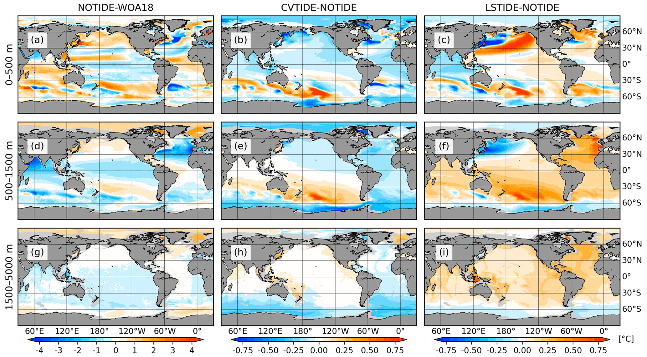
Figure 1Depth-averaged temperature biases between the model results and WOA18 in the upper (0–500 m), intermediate (500–1500 m) and deep (1500–5000 m) ocean. Panels (a), (d) and (g) show the biases between NOTIDE and WOA18, and the other panels show the differences between the sensitivity runs and the control run. Opposite colours in panel (a) and panel (b)/(c) indicates that CVTIDE/LSTIDE reduces temperature biases in NOTIDE and so on.
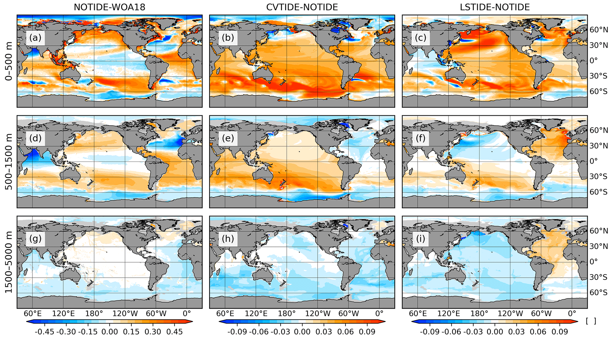
Figure 2The same as Fig. 1 but for salinity.
The tidal effects also demonstrate improvements to different extents at different depths of each basin. Figure 3 shows basin-averaged temperature and salinity biases at each vertical layer in the model. In the left panels, LSTIDE shows significant improvements to the temperature biases in the Pacific, Atlantic, and Indian oceans deeper than 1000 m. CVTIDE only reduces temperature biases in the Arctic Ocean at 500–2000 m in depth. Also, both CVTIDE and LSTIDE reduce temperature biases in the Southern Ocean deeper than 4000 m. In the right panels, we can only find improvements in LSTIDE. Salinity biases are slightly reduced in the Atlantic and Pacific oceans, around 1500 m in depth. We should also note that in Fig. 3j, significant salinity biases emerge on the surface Arctic Ocean. These result from the differences between the PHC3 and WOA datasets. Our model starts with the PHC3 climatology, which integrates the WOA dataset and the Arctic Ocean Atlas.
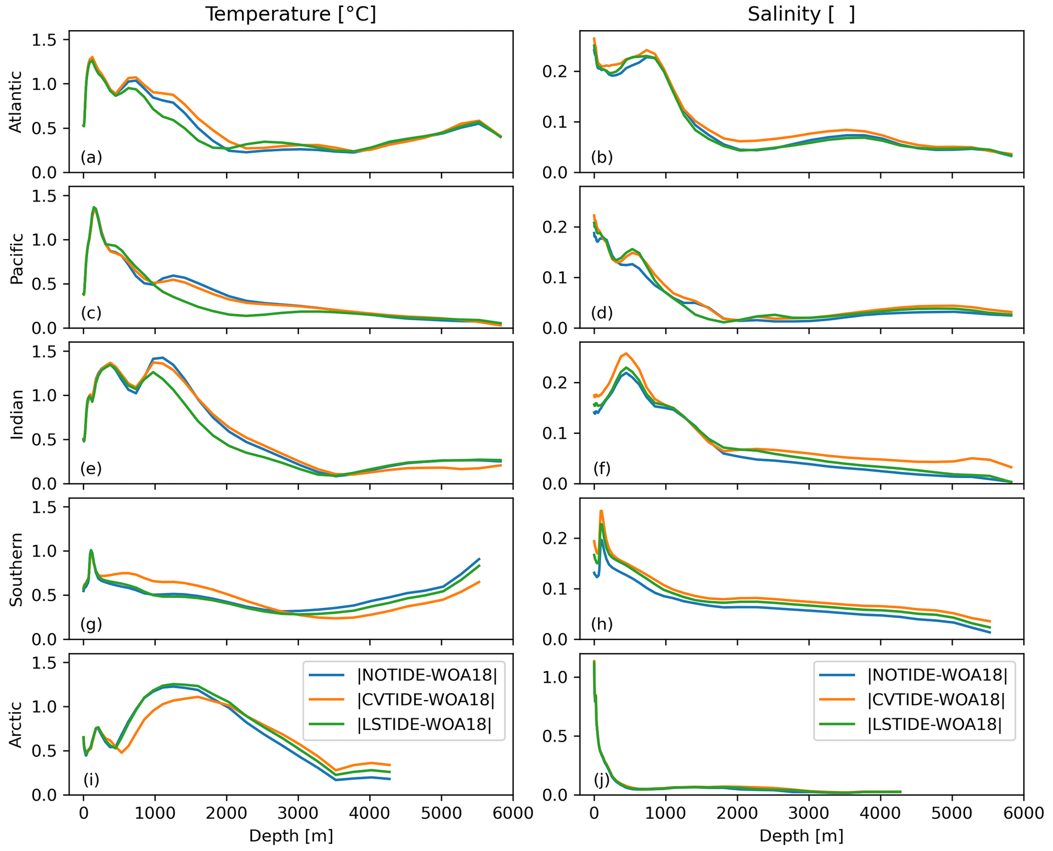
Figure 3Basin-averaged hydrographic biases between the model results and WOA18 with respect to water depths. The hydrographic biases are absolute values. Panels (a), (c), (e), (g) and (i) and panels (b), (d), (f), (h) and (j) represent temperature and salinity biases, respectively, while each row shows the biases in different basins. The averaging is nodal-area-weighted.
CVTIDE and LSTIDE also greatly influence the hydrography in the continental shelf and slope areas, which cannot be clearly shown in Figs. 1–3. By assembling grids with the same bathymetry and averaging the temperature and salinity biases, the bathymetry-averaged biases with respect to depths are shown in Fig. 4. In Fig. 4a, the model results in the control run demonstrate significant temperature biases near continental shelf and slope topographies, and both CVTIDE and LSTIDE decrease the biases in these areas. By comparing Fig. 4c with Fig. 4e, CVTIDE has a better improvement near the bottom of the continental shelf and slope, while LSTIDE significantly reduces temperature biases at 1000–4000 m in depth, which is not shown in CVTIDE. In Fig. 4b, significant salinity biases in the control run concentrate in the shallow continental shelf areas. It is shown in Fig. 4d and f that CVTIDE decreases salinity biases at the near-bottom continental shelf area, while LSTIDE decreases salinity biases in the whole layer of the continental shelf area. Neither of the two comparison runs demonstrates a significant improvement to other areas, except for the slight modification of LSTIDE around 1500 m in depth.

Figure 4Bathymetry-averaged hydrographic biases between the model results and WOA18 with respect to water depths. The hydrographic biases are absolute values, and model mesh grids with the same bathymetry (maximum water depth) are assembled and averaged. Panels (c)–(f) are presented to show the differences with panels (a) and (b); thus the blue/red colours indicate that tidal effects decrease/increase model biases in the control run. The averaging is nodal-area-weighted, and the axes are scaled with a cube root.
3.2 Sea ice
Figure 5 shows the results of sea ice thickness (SIT) in the polar regions. Both tidal effects alter the sea ice results, but the patterns are different.
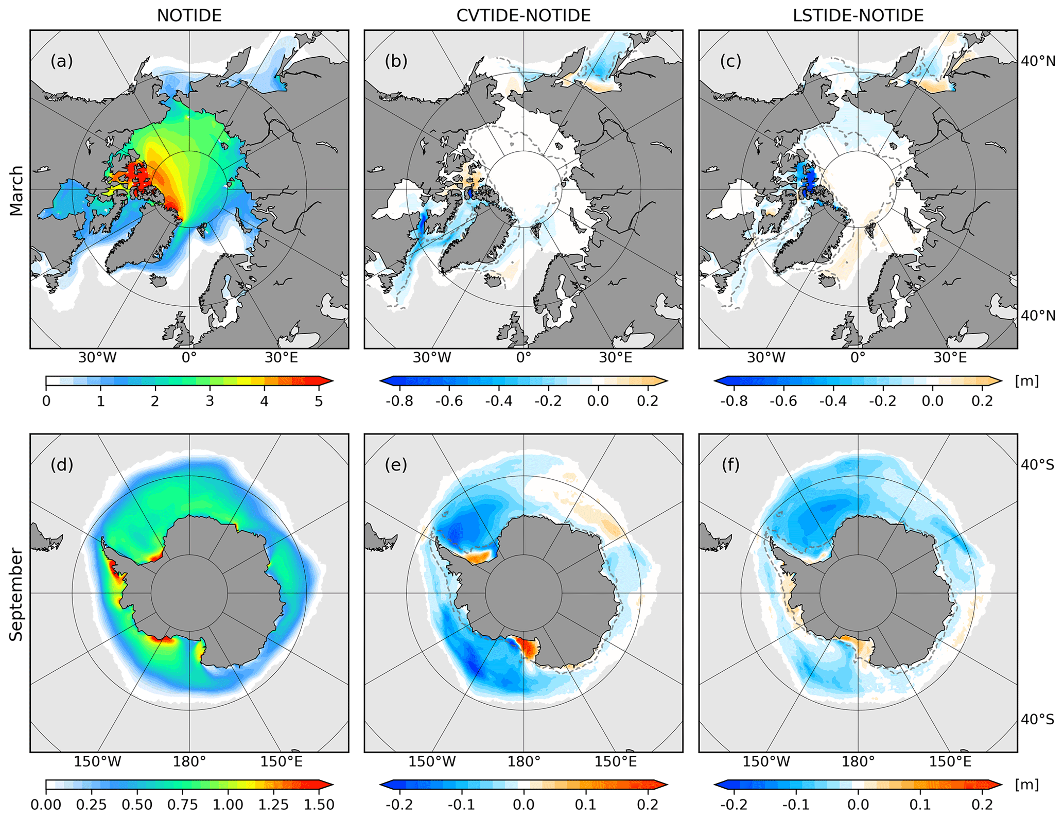
Figure 5Polar sea ice thickness in the three sensitivity runs. Panels (a) and (d) show the results from the control run, and the other panels show the differences. Panels (a)–(c) and (d)–(f) show the Arctic (March) and Antarctic (September) results. The grey backgrounds mask the ice-free areas, and the dashed grey line represents the 500/1000 m isobath for panels (a)–(c)/(d)–(f).
In the Arctic region, CVTIDE generally decreases SIT in the Labrador Shelf, East Greenland Shelf and the Sea of Okhotsk but increases SIT in the Canadian Arctic Archipelago (CAA). LSTIDE shows a slighter SIT decrease than CVTIDE in the Sea of Okhotsk and Labrador Shelf but increases SIT in the Greenland Sea. One of the most significant differences between LSTIDE and CVTIDE is that LSTIDE shows a remarkable SIT decrease in the CAA. The mean SIT in the CAA in the control run is 6.01 m; LSTIDE decreases by 0.60 m, while CVTIDE increases by 0.03 m. In the Antarctic region, both CVTIDE and LSTIDE show similar patterns, including a general SIT decrease around Antarctica and an SIT increase on the Weddell Sea continental shelf and Ross Sea continental shelf. On the West Antarctic Peninsula Continental Shelf, SIT decreases in CVTIDE but increases in LSTIDE. Generally speaking, CVTIDE shows a more significant impact on SIT than LSTIDE.
We should also point out that CVTIDE consistently reduces SIT in both regions at shelf-break areas, which are indicated by the dashed grey lines. However, LSTIDE does not show this consistency. The difference is further discussed in Sect. 4.
3.3 Meridional overturning circulation
The left column of Fig. 6 shows that CVTIDE and LSTIDE affect AMOC differently. CVTIDE weakens the AMOC upper cell by 0.50 Sv and strengthens the lower cell by 0.75 Sv, while LSTIDE strengthens the AMOC upper cell by 1.50 Sv and weakens the lower cell by 0.25 Sv. That indicates CVTIDE weakens the North Atlantic Deep Water (NADW) formation and strengthens the Antarctic Bottom Water (AABW) formation, while LSTIDE behaves the opposite.
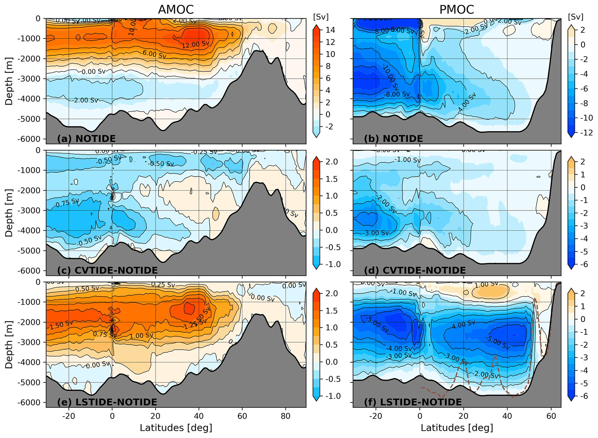
Figure 6The MOC results in the three sensitivity runs. Panels (a) and (b) show the results from the control run, and the other panels show the differences. Panels (a), (c) and (e) and panels (b), (d) and (f) represent AMOC and PMOC, respectively. The dashed brown line in panel (f) denotes the North Pacific topography along the 180∘ transect. All the MOC contains the vertical component of bolus velocities (Gent and Mcwilliams, 1990). The calculation of MOC in the unstructured mesh applies the algorithm introduced in Sidorenko et al. (2020).
The results of PMOC are shown in the right column of Fig. 6. The main effect of CVTIDE on the PMOC occurs in the south Indo-Pacific Ocean. The deep water upwelling at 20∘ S is enhanced by 4 Sv. LSTIDE has a more significant effect than CVTIDE. Figure 6f features two cells: the south cell upwells deep water in the tropical Indo-Pacific Ocean, while the north cell upwells deep water in the subarctic North Pacific Ocean. Both cells enhance deep water upwelling by 5 Sv, and the upwelled deep waters are released to the Indo-Pacific Ocean's intermediate layer (about 1000–2000 m). The north cell in Fig. 6f shows consistency with the North Pacific bathymetry, which is further discussed in Sect. 4.
3.4 Vertical diffusivity
Since tidal mixing is stimulated by topographies, tidal mixing and vertical diffusivity are bottom-enhanced. Figure 7a–c show the near-bottom vertical diffusivity in the three sensitivity runs. Compared with the control run, Fig. 7b shows observably that the CVMIX_TIDAL parameterisation enhances vertical diffusivity by a large value in the deep ocean. In CVTIDE, the vertical diffusivity is enhanced where bottom topography roughness is large, such as seamounts, deep ocean ridges and shelf-break areas. The pattern of LSTIDE is very different compared with CVTIDE, and we cannot see a coherent enhancement of vertical diffusivity in the near-bottom ocean. The global mean vertical diffusivity profiles (Fig. 7d) also demonstrate that compared with CVTIDE, LSTIDE does not enhance vertical diffusivity significantly in the deep ocean.
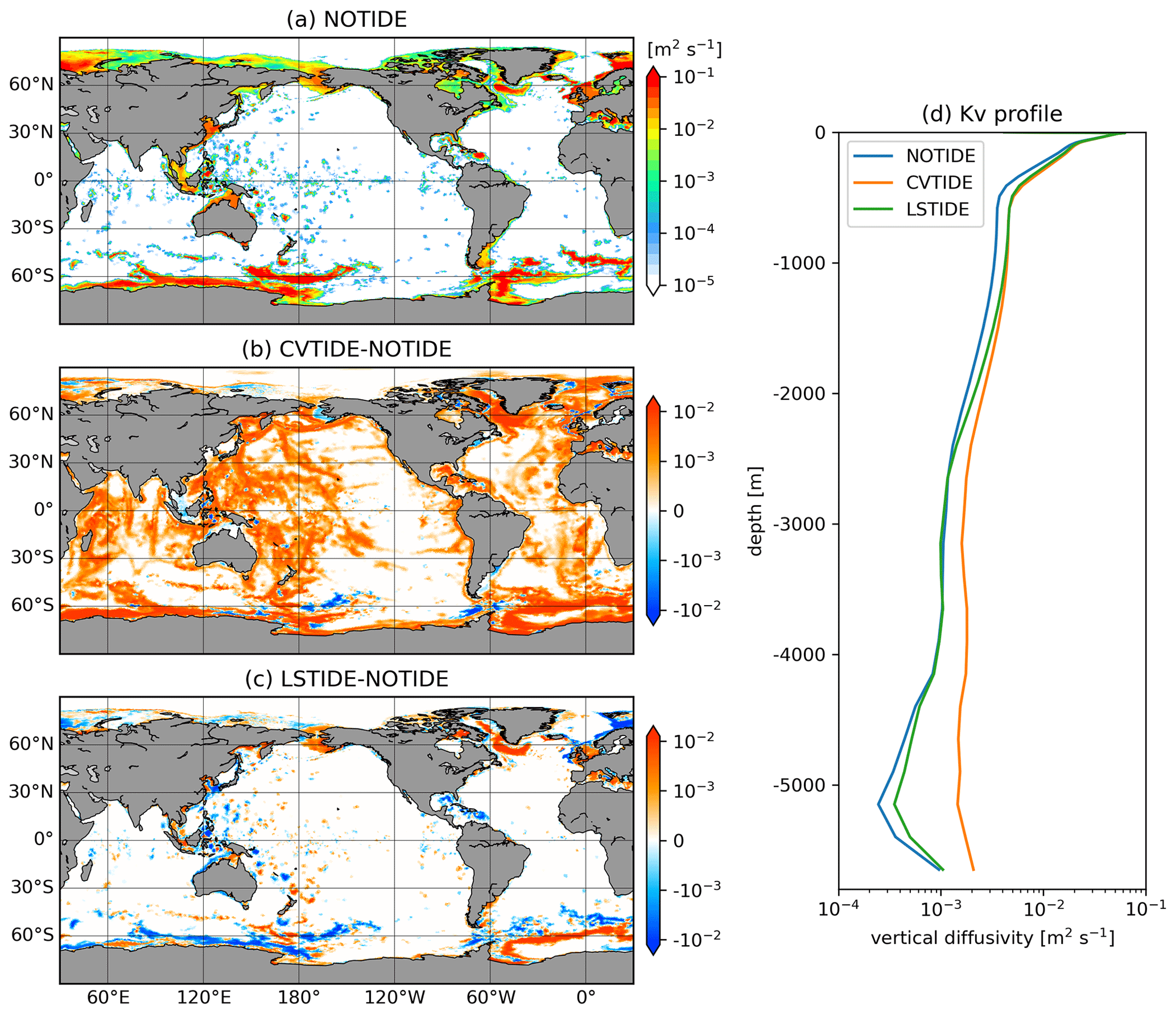
Figure 7Panels (a)–(c) are horizontal maps of depth-averaged vertical diffusivity over the bottom 500 m (average over the whole depth where bathymetry is less than 500 m). Panel (d) shows the global mean vertical diffusivity profile in the three sensitivity runs. Colour bars are shown in decimal logarithmic scales.
3.5 Barotropic streamfunction
Figure 8 demonstrates that CVTIDE and LSTIDE show similar patterns in changing the global barotropic streamfunction. The patterns of streamfunction differences in Figs. 8b and 8c mainly consist of two loops. The “blue loop” is mainly located in the Indo-Pacific Ocean: the southward transport enhances the ITF and finally contributes to the ACC, and its recirculation is located in the western Pacific Ocean. The “red loop” enhances the ACC separately. The blue and red loops are stronger in LSTIDE than those in CVTIDE. CVTIDE enhances the ITF and the ACC through the Drake Passage by 1.72 and 4.79 Sv, while the values of LSTIDE are 3.92 and 10.34 Sv, respectively. In addition, we can find an essential difference regarding the blue loop: the blue loop extends to the subpolar Pacific Ocean and the South Atlantic Ocean in LSTIDE but not in CVTIDE. The difference determines the PMOC–AMOC connection, which is discussed in Sect. 4.
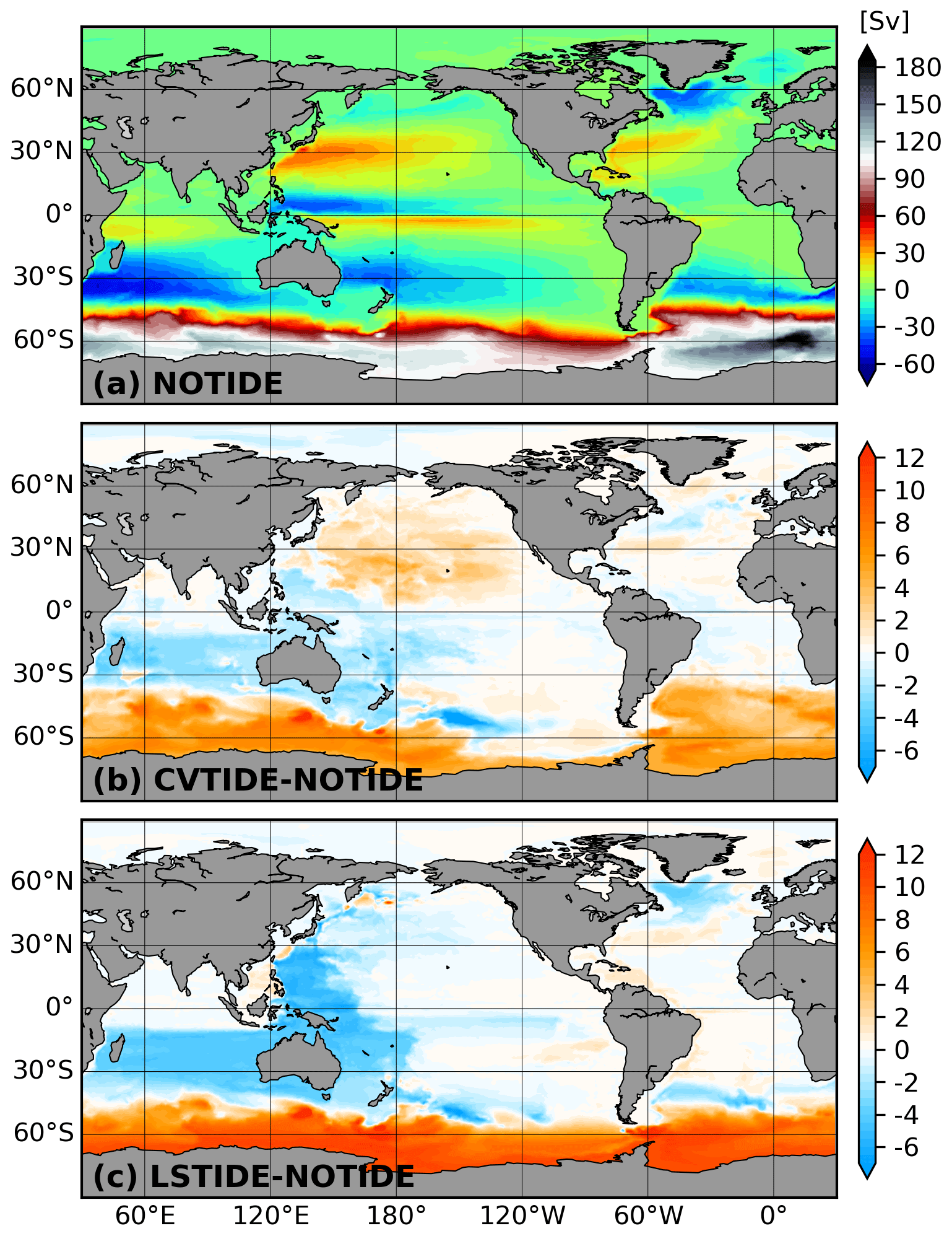
Figure 8The barotropic streamfunction in the three sensitivity runs. Panel (a) shows the result in the control run, while panels (b) and (c) show the differences. Panel (c) also represents the tidal residual mean circulation. The calculation of barotropic streamfunction in the unstructured mesh applies the algorithm introduced in Sidorenko et al. (2020).
3.6 Energy
Based on the energy budget equation (see Appendix B1), we diagnose the energy terms from the model results and list the global integration values in Table 1. Due to the additional energy input in LSTIDE (Tide and KE in Table 1), three energy dissipation terms (bottom drag, vertical viscous dissipation and horizontal viscous dissipation) are enhanced compared with NOTIDE and CVTIDE, especially for bottom drag. The additional energy sink in these three terms accounts for about 1 TW. The remaining 3.5 TW of the total 4.6 TW tidal potential power is converted from kinetic energy to barotropic potential energy.
Table 1A global integration of kinetic energy budget from the model results. The surface wind stress, bottom stress, vertical viscous dissipation, horizontal viscous dissipation, buoyancy flux, tidal potential power (Tide), the barotropic potential energy–kinetic energy conversion term (PE2KE) and total kinetic energy (KE) are listed in order in the table. The expressions of these terms can be found in Appendix B1. All except the last term have a unit of terawatts (TW), while kinetic energy has a unit of 1018 J.
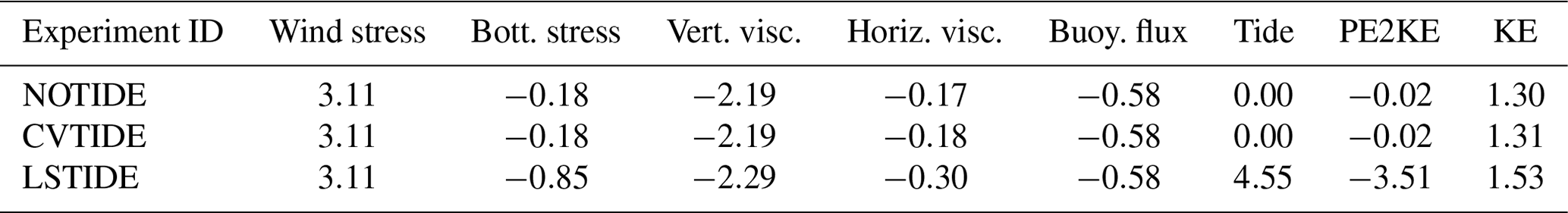
Figure 9 shows the horizontal distribution of vertically integrated bottom drag and viscous dissipation. Because of the strong tidal currents in marginal seas and continental shelf areas, LSTIDE enhances bottom drag and viscous dissipation significantly in these areas. Like the vertical diffusivity, the vertical viscosity is also enhanced in the CVMIX_TIDAL parameterisation, but the effect is negligible (Fig. 9e).
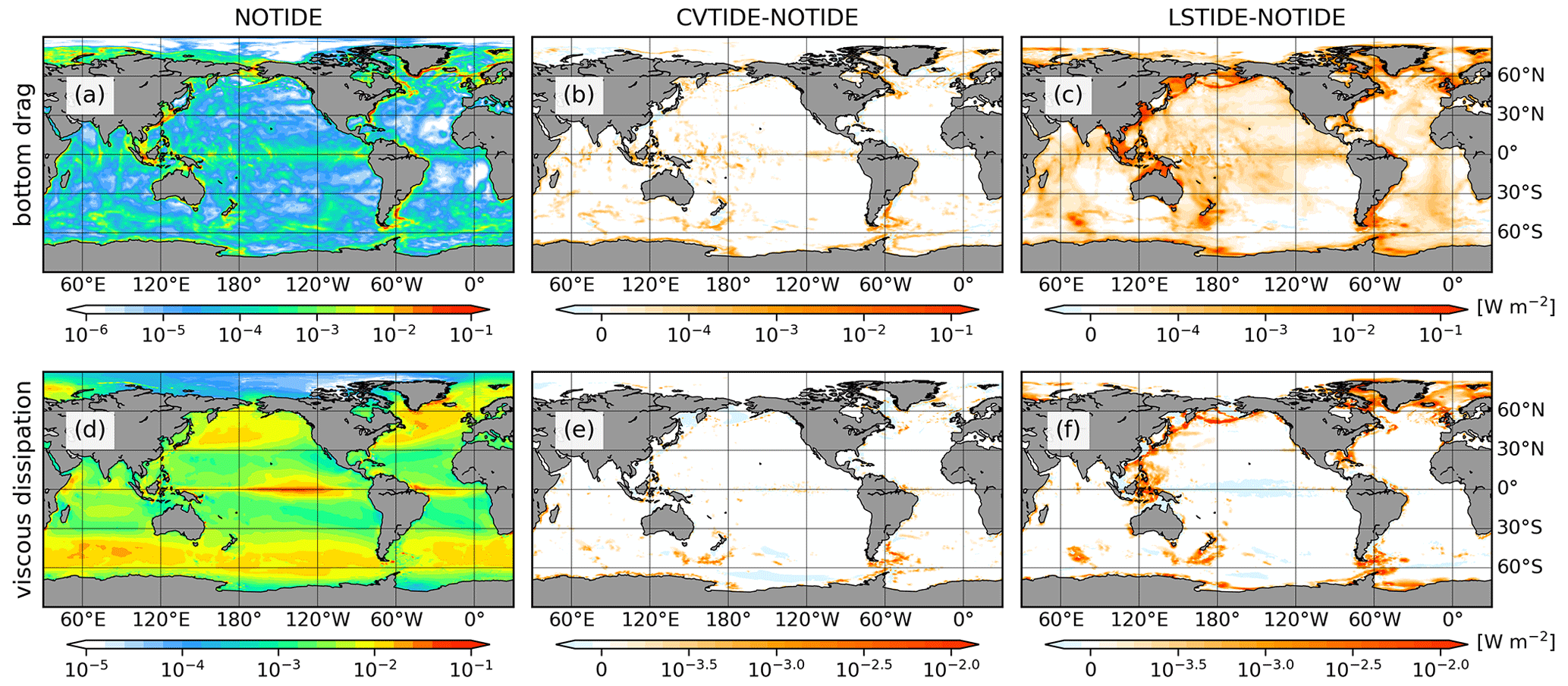
Figure 9Horizontal distribution of vertically integrated energy dissipation terms in Table 1 (we change the sign so that positive values represent energy dissipation). Panels (a)–(c) and (d)–(f) indicate bottom drag and viscous dissipation (including horizontal and vertical components), respectively. Panels (a) and (d) show the control run, and the other panels show the differences. Colour bars are shown in decimal logarithmic scales.
Even though the global integration of buoyancy flux shows no difference in the three runs, the horizontal distribution shows differences (Fig. 10). Regional integration values over the Kuril–Aleutian Ridge area (120∘ E–120∘ W, 30∘ N–60∘ N) in NOTIDE, CVTIDE and LSTIDE are −1.22, −1.52 and −2.78 TW, respectively. In the Indonesian Archipelago area (90–150∘ E, 15∘ S–15∘ N), regional integration values in NOTIDE, CVTIDE and LSTIDE are −0.82, −1.13 and −1.19 TW, respectively. Compared with CVTIDE, LSTIDE shows a stronger enhancement of buoyancy flux in the Kuril–Aleutian Ridge and Indonesian Archipelago but a weaker enhancement in other mid-latitude areas. The lower panels of Fig. 10 indicate that with tidal currents in LSTIDE, turbulent buoyancy flux plays an essential role in the oceanic mixing and buoyancy flux (see Appendix B2).

Figure 10Horizontal distribution of vertically integrated buoyancy flux terms. Panels (a)–(c) and (d)–(f) indicate buoyancy flux and turbulent buoyancy flux, respectively. Buoyancy flux in this figure is expressed as gρw, while turbulent buoyancy flux is (positive values represent upwelling). Panels (a) and (d) show the control run, and the other panels show the differences.
4.1 The effect of resolution on tidal mixing
As shown in Munk and Wunsch (1998) (their Fig. 4), internal tides are important links between surface tides and oceanic mixing. Indeed, Niwa and Hibiya (2011, 2014) demonstrate that the conversion rate of internal tide energy in a global tide model depends on the model resolution. Thus, if the model mesh cannot resolve internal tides, the internal-tide-induced mixing is missing in the model result. Figure 11 presents the ratio of mode-1 internal tide wavelengths to the mesh resolution. We can find that most of the model areas cannot resolve propagating internal tides in the mid-latitude area, especially for semidiurnal ones in Fig. 11b. In addition, even though the unstructured model mesh has a higher resolution in shelf-slope areas, it still cannot resolve internal tides therein because the wavelengths of internal tides are smaller in these areas. So we infer that LSTIDE has a strong dependence on the model resolution.
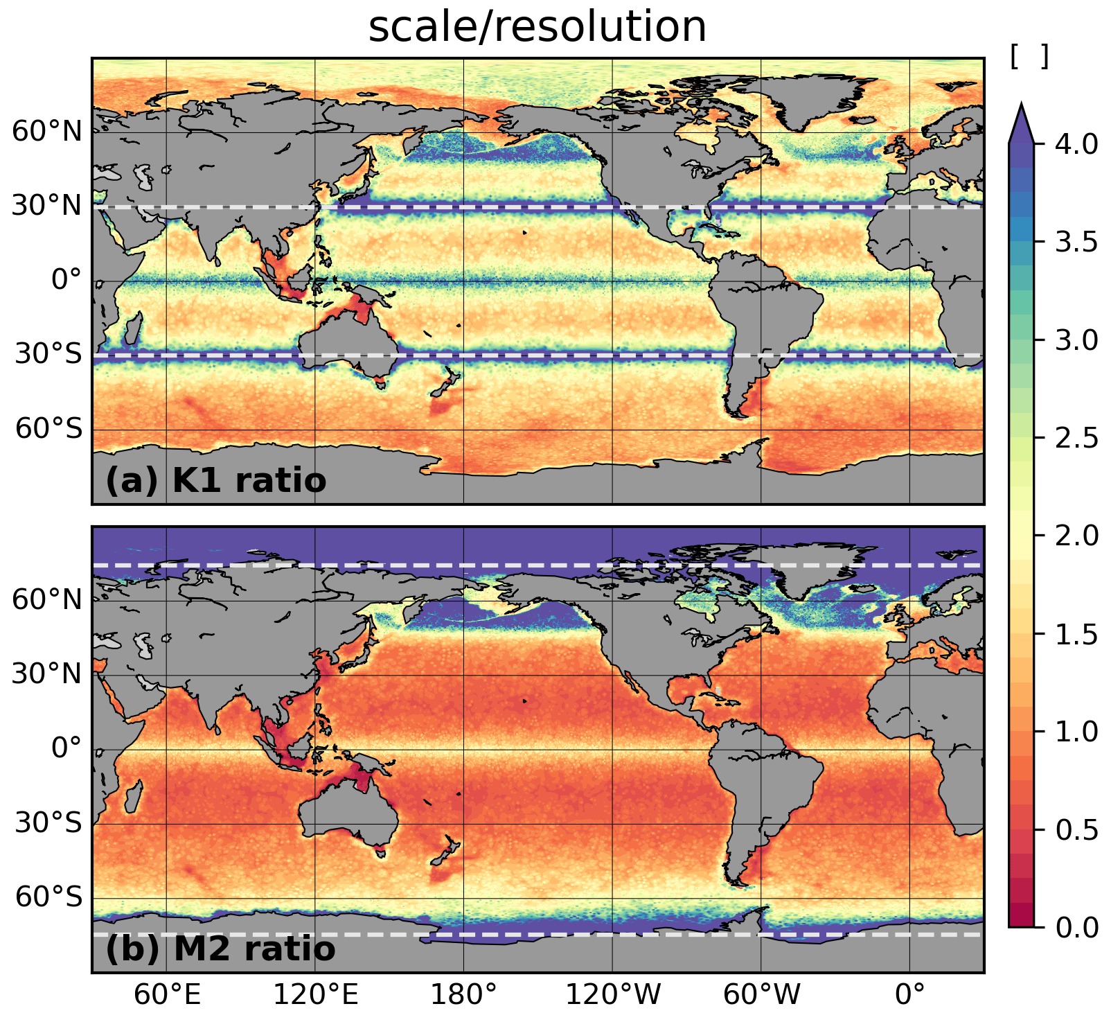
Figure 11The ratio of mode-1 K1/M2 internal tide scale and mesh resolution. The dashed thick grey line indicates the critical latitudes of internal tides. The calculation of internal tide scale is introduced in Appendix B3.
Evidence can be found in the model results. In Fig. 4, compared with CVTIDE (Figs. 4c and d), LSTIDE (Figs. 4e and f) shows a weaker reduction of hydrographic biases near the bottom of shelf breaks. The internal tides at shelf-slope areas cannot be resolved in LSTIDE, which weakens the mixing effect. Tidal mixing on shelf breaks also affects SIT. Unlike other places where the temperature decreases monotonically with depth, the polar regions have colder water near the surface than in the deeper layers. Thus in polar regions, the tidal mixing on shelf-slope areas would lead to a warmer surface ocean, which should decrease the SIT. In our result, LSTIDE shows a smaller SIT decrease than CVTIDE on the shelf-slope area, such as the Labrador Shelf and the Antarctic continental shelf (Fig. 5). The effect of the resolution is also reflected in the model vertical diffusivity. Both observational results (Polzin et al., 1997) and CVMIX_TIDAL parameterisation suggest larger vertical diffusivities near the bottom, which is caused by the tide–topography interaction. However, vertical diffusivities in the near-bottom layers are not generally higher in LSTIDE than in NOTIDE (Fig. 7c). The lack of resolving internal tides causes the underestimation of vertical shear, thus leading to a different result compared with CVTIDE. The buoyancy flux results (Fig. 10b and c), which are most directly connected to oceanic upwelling, also show weaker mixing effects in mid-latitude areas in LSTIDE compared with CVTIDE. Figure 11 shows the model mesh can roughly resolve propagating internal tides in tropical areas, where strong mixing can be found in LSTIDE. LSTIDE (Fig. 6f) shows strong mixing and upwelling in the equatorial Indo-Pacific Ocean, which is not clearly shown in CVTIDE (Fig. 6d). We think this comes from the underestimation of tidal dissipation efficiency (q). The tidal dissipation efficiency is set to 0.33 in this work, but previous work indicates higher efficiencies in the Indonesian Archipelago area (Koch-Larrouy et al., 2007; Nagai and Hibiya, 2015).
Figure 11 also implies trapped internal tides beyond critical latitudes. According to the dispersion relationship of internal tides, where the inertial frequency is higher than a tidal frequency (f>ω), internal tides at the tidal frequency would not have a wave solution, resulting in trapped internal tides instead of propagating internal tides (latitudes higher than the dashed lines in Fig. 11). Unlike propagating internal tides, trapped internal tides can only be dissipated in a small domain, leading to a higher local dissipation rate and thus stronger local mixing. The Kuril Ridge and Aleutian Ridge, which connect the Sea of Okhotsk and the Bering Sea with the North Pacific Ocean, are the main generation sites for trapped diurnal internal tides. Large dissipation rates by trapped internal tides are validated in previous modelling research (Niwa and Hibiya, 2011, 2014; Tanaka et al., 2010, 2013; Falahat and Nycander, 2015), and intense mixing is also observed therein (Nakamura et al., 2010; Itoh et al., 2014).
LSTIDE demonstrates intense mixing in the Kuril Ridge and Aleutian Ridge, resulting in higher buoyancy flux than NOTIDE in these areas (Fig. 10c). LSTIDE does not change the vertical diffusivity significantly. Still, it enhances the upwelling in the North Pacific. We explain this by tide-induced turbulent buoyancy flux (Fig. 10f and Appendix B2). The strong mixing upwells an additional 5 Sv of deep water in the North Pacific (around 50∘ N) to the intermediate layer and then spreads to the south (Fig. 6f). The strong mixing in the Indonesian Archipelago also results in strong upwelling. The upwelled water from both the Indonesian Archipelago and Kuril–Aleutian Ridge contributes to the ITF (Fig. 8c) and flows into the Indian Ocean. Stronger PMOC helps to reduce temperature biases in the intermediate Indo-Pacific Ocean (Fig. 1f): the upwelling of the deep water reduces the warm biases in the North Pacific Ocean and cold biases in the tropical Indo-Pacific Ocean in NOTIDE.
Trapped internal tides and related mixing can be simulated with LSTIDE because in the high-latitude areas, the CORE-II mesh is fine enough to resolve trapped internal tides (Fig. 11). As a comparison, even though CVTIDE does not show much influence on the PMOC in the North Pacific Ocean, it shows similar but weaker patterns in reducing the temperature biases in the intermediate layer. This is probably for two reasons: (1) most of the trapped internal tides' energy is dissipated locally, so the tidal dissipation efficiency is close to unity (q≈1) in this area instead of 0.33 from CVTIDE, and (2) the simulation is not long enough to become stable. It should also be emphasised here that even though the PMOC lower cell in the North Pacific is reported in most previous work (e.g. Simmons et al., 2004; Oka and Niwa, 2013), our results in LSTIDE demonstrate a different shape for the PMOC lower cell in the North Pacific. The significant upwelling occurs in the Aleutian Ridge, and the upwelling has great consistency with the topography (take the brown transect in Fig. 6f as an example). The diurnal tidal mixing beyond critical latitudes causes an upwelling along the bottom boundary, which is not reported in previous work. Nevertheless, our result supports some previous arguments (Scott and Marotzke, 2002; Ferrari et al., 2016) that the upwelling caused by near-boundary mixing is more important than interior mixing in closing the THC.
4.2 The tidal effects on the global THC
The model also shows interesting results in the spin-up. The time series of several main constituents of the global THC is demonstrated in Fig. 12. In Fig. 12a and b, we find that both CVTIDE and LSTIDE show a stronger PMOC and ITF than the control run from the beginning. In the fourth and fifth cycles, the discrepancies of PMOC and ITF between CVTIDE/LSTIDE and NOTIDE become stable. In Fig. 12c, it is shown that in the first cycle, the strength of AMOC upper cell in both CVTIDE and LSTIDE is weaker than that in the control run. However, from the second cycle, the strength of the AMOC upper cell in LSTIDE starts to surpass that in NOTIDE. The strength of the AMOC upper cell in CVTIDE is weaker than that in NOTIDE in all cycles. As mentioned in Sect. 2, the CVMIX_TIDAL scheme applies the same formula to the model viscosities, potentially increasing model dissipation and leading to a weaker circulation on shelf-slope areas. Thus, the wind-driven circulation, the poleward heat flux and the AMOC upper cell are weakened, which corresponds with previous work (e.g. Jayne, 2009; Yu et al., 2016). But a major difference between CVTIDE and LSTIDE embodies the subsequent enhancement of the AMOC upper cell in LSTIDE. Results from LSTIDE reveal that the upwelling in the North Pacific and Indonesian Archipelago is linked to the North Atlantic. Figures 6f and 8c indicate that the enhancement of mixing in the North Pacific and Indonesian Archipelago results in a stronger PMOC and ITF. The ITF mass transport finally forms the blue loop in the barotropic streamfunction difference (Fig. 8c). The westernmost part of this loop extends to the South Atlantic, which seems to have no connection with the North Atlantic. But note here that the vertical structure of oceanic circulation cannot be revealed by the barotropic streamfunction. Nevertheless, Fig. 6e further shows that the upper cell of AMOC is enhanced, and the effect originates from the South Atlantic. Conversely, even though CVTIDE also has a stronger ITF and a blue loop streamfunction difference, it does not strengthen the upper cell of AMOC because the blue loop is restricted in the Indo-Pacific Ocean and does not extend to the South Atlantic (Fig. 8b). The connection between the Indo-Pacific Ocean and the Atlantic Ocean is the Agulhas leakage. The Agulhas leakage is strengthened in LSTIDE (Fig. 8c), but the pattern is cut off in CVTIDE (Fig. 8b). And that explains why the strengthening of PMOC and ITF only leads to AMOC increase in LSTIDE. The importance of Agulhas leakage in connecting cross-basin circulation is also reported in Biastoch et al. (2008). In addition, we rule out the possibility that the tidal mixing in the Atlantic itself causes the strengthening of the AMOC upper cell for two reasons: (1) in Fig. 6e, the AMOC cell does not show a closed overturning circulation, which means 1.5 Sv of AMOC is not upwelled in the Atlantic Ocean north to 30∘ S, and (2) the transect plot does not show either stronger vertical diffusivity or turbulent buoyancy flux in the Atlantic Ocean (figure not shown). The cycle revealed in our result corresponds well with a previous paper (Talley et al., 2011, their Fig. S14.1c). The enhancement of ITF due to tidal mixing is also reported in previous research (Schiller, 2004; Sasaki et al., 2018), and the link between the stronger PMOC lower cell and the stronger AMOC upper cell can also be found in Melet et al. (2016).
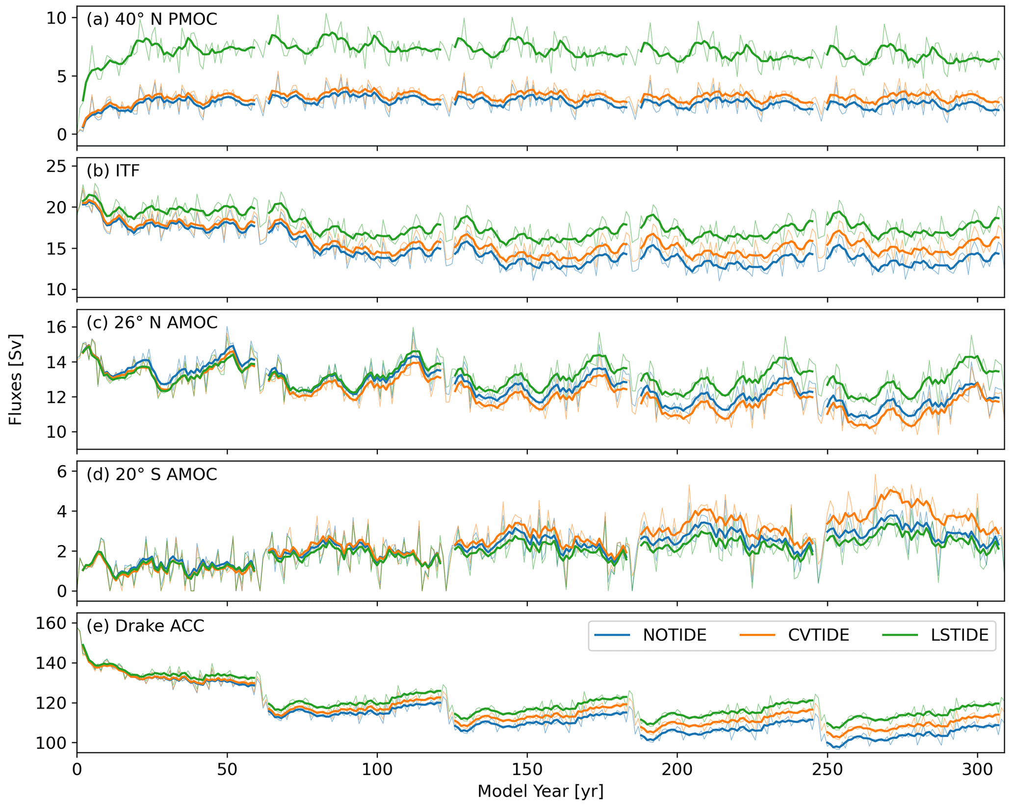
Figure 12The time series of (a) 40∘ N PMOC, (b) ITF, (c) 26∘ N AMOC, (d) 20∘ S AMOC and (e) ACC through the Drake Passage from the three sensitivity runs in all five cycles. The light and thin lines are original annual time series, and the dark and thick lines are 5-year moving average results for each cycle. Note that 26∘ N AMOC and 20∘ S AMOC denote the strength of the AMOC upper cell and lower cell, respectively. The calculation of ITF and ACC flux through the transects in the Indonesian Archipelago and the Drake Passage applies the algorithm introduced in Sidorenko et al. (2020).
As for the AMOC lower cell, LSTIDE shows a weakening effect, while CVTIDE shows a strengthening effect (Fig. 12d). It is widely believed that the global tidal mixing and wind-driven upwelling in the Southern Ocean affect the MOC (Ledwell et al., 2000; Marshall and Speer, 2012). Since the model configuration applies the same atmospheric forcing in the three sensitivity runs, the reason concerning wind stress would be excluded. Moreover, considering the vertical advection–diffusion balance (Munk and Wunsch, 1998; Prange et al., 2003), the tidal mixing should strengthen the MOC, as CVTIDE shows. As discussed above, LSTIDE has the disadvantage of demonstrating tide-induced mixing in the vast mid-latitude areas due to the resolution; thus, the AMOC lower cell is weakened instead of strengthened in LSTIDE. We also suspect that the enhanced vertical diffusivities may be added to deep convection areas, directly leading to stronger convection. However, the CVMIX_TIDAL parameterisation implies that the enhanced vertical diffusivities are not added to areas where gravitational instability occurs (N2<0). So we finally conclude that the AMOC lower cell is enhanced due to tidal mixing, and more AABW formation in the Weddell Sea is a result instead of a reason for the strengthening of the AMOC lower cell. A similar conclusion can be found in Exarchou et al. (2012).
CVTIDE and LSTIDE also demonstrate that the ACC transport through the Drake Passage is larger than that in NOTIDE (Figs. 8 and 12e). We can see from Fig. 12e that the strength of ACC in all three sensitivity runs decreases during the five cycles, but the decreasing rate is lower in the comparison runs, which can be explained by Fig. 13. Figure 13d and f show that both comparison runs have similar effects on changing potential density in the Southern Hemisphere. In the mid- and low-latitude areas, both tidal effects demonstrate denser seawater in the upper ocean and lighter seawater in the lower ocean, indicating the promotion of ocean potential energy caused by the tidal mixing. In the high-latitude areas, both comparison runs show denser seawater from the surface to the bottom, indicating the reduction of ocean potential energy due to the deep convection. In depths below 1000 m, both CVTIDE and LSTIDE show potential density decrease at subtropical latitudes. The decrease in potential density is caused by the mixing and advection effect indicated by the global MOC (GMOC). For example, Fig. 13e shows that strong mixing and upwelling take place in the tropical region, and the upwelled water further advects to the south (similar to Fig. 6f). The advection effect causes the “blue tongue” pattern in Fig. 13f (1000–2000 m in depth). In addition, the potential density increase at subpolar latitudes can be explained by the AABW formation. In the above context, our results show that the tidal mixing in CVTIDE causes the strengthening of the AABW formation. This is also why the potential density increase at subpolar latitudes is more substantial in CVTIDE than in LSTIDE. Even though CVTIDE and LSTIDE alter potential density differently, both experiments increase the meridional density gradients in the Southern Ocean, which prevents the strength of ACC from decreasing due to the thermal wind relation. Thus we conclude that both CVTIDE and LSTIDE affect the ACC strength by enhancing the meridional density gradient. Similar results are also shown in Saenko and Merryfield (2005) that with tidal mixing parameterisation, the ACC transport is stronger by 25 % compared with their control run.
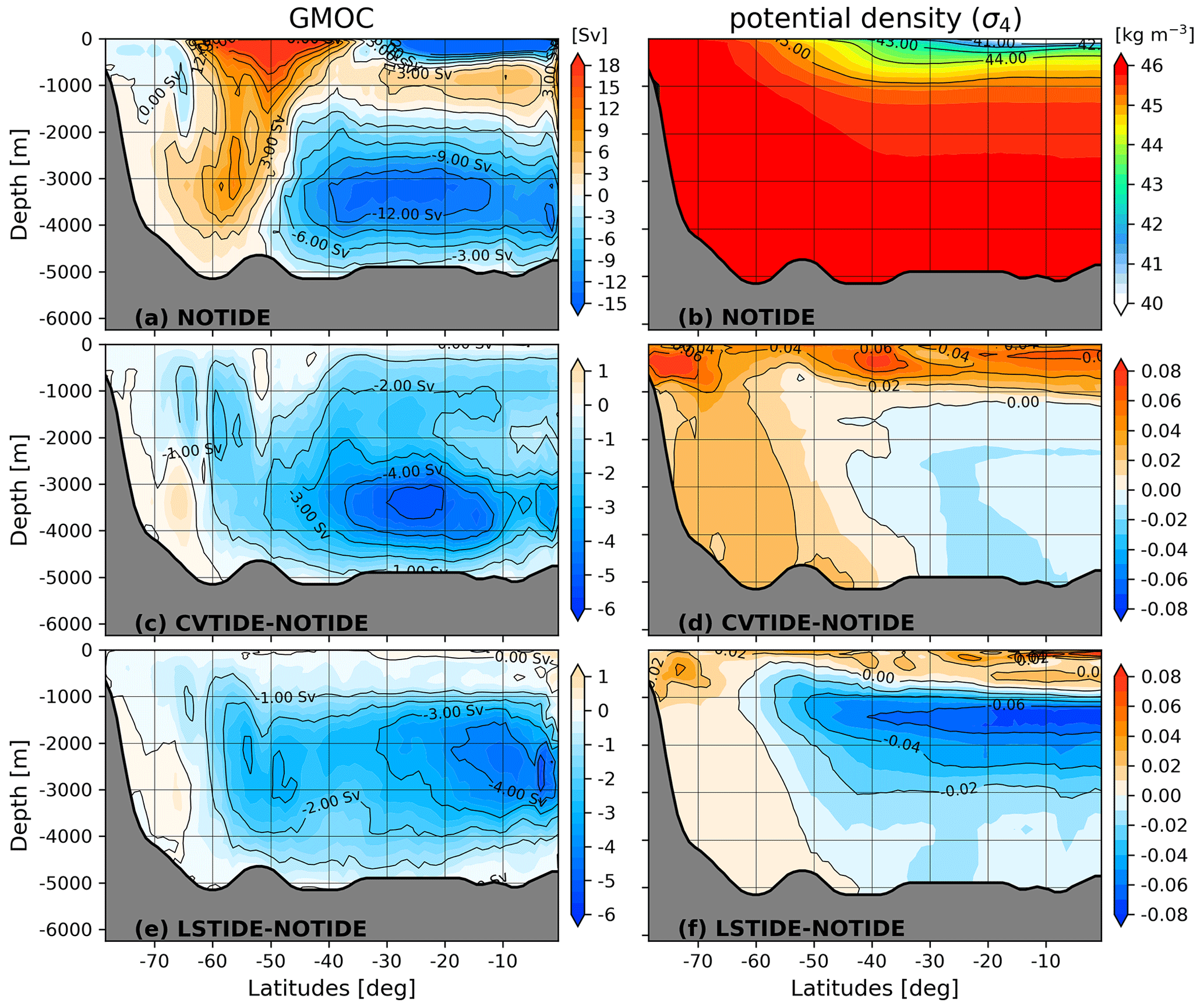
Figure 13The GMOC and potential density with reference depth at 4000 m (σ4) in the Southern Hemisphere. Panels (a) and (b) denote results in the control run, and the other panels denote the differences. The potential density is globally zonal averaged, with the meridional bin set to 1∘.
4.3 Other tidal effects: what does CVTIDE miss?
The “barotropic tide–baroclinic tide–oceanic mixing” chain is considered the most crucial tidal effect on the ocean and climate. But we are still questioning if there are any effects from tides other than internal tide mixing. Since CVTIDE only considers internal tide mixing effects, and LSTIDE considers real-tide effects, we can answer this question by comparing LSTIDE with CVTIDE.
The most significant difference is the energy in the model. If the tidal potential term is added to the ocean primitive equation, tide energy is thus input to the system (Table 1). The global tidal potential power is 4.6 TW in our model. However, most of the energy goes to the barotropic potential energy, indicating a lack of internal tides in the system. If the model resolved more internal tides, the surface tide amplitudes and the conversion to barotropic potential energy would be smaller due to the internal wave drag (e.g. Jayne and St. Laurent, 2001; Sulzbach et al., 2021). This part of energy would be redistributed to the buoyancy flux and energy dissipation terms, depending on the conversion rate between surface tides and internal tides. External energy input not only leads to higher kinetic energy but also higher energy dissipation. Comparing Fig. 9b with Fig. 9c, we find that the bottom drag is significantly enhanced in LSTIDE compared to CVTIDE. Regarding the viscous dissipation, LSTIDE shows remarkable enhancement on continental shelves (Fig. 9f), while CVTIDE does not show significant changes compared with NOTIDE. The reason is that LSTIDE has strong tidal shear caused by the bottom drag of barotropic tides on continental shelves, while CVTIDE only increases viscosity and diffusivity on shelf breaks and seamounts, indicating an effect of internal tides.
Additionally, we find that considering the strong tidal shear on continental shelves can reduce model biases. Both Figs. 4e and 4f indicate that in LSTIDE, the temperature and salinity biases on continental shelves (e.g. bottom depth less than 100 m) are better reduced compared with CVTIDE. Via a coupled climate model, Lee et al. (2006) also found that local hydrographic biases can be reduced when considering tidal shear effects on continental shelves.
From a mathematical point of view, adding periodic tidal motions can also affect stress terms, leading to a tidal residual effect. Even though tidal velocities can roughly be eliminated via time-averaging, the stress terms can always leave non-zero cross terms. These effects are more remarkable in regional simulations than global ones. Our results show that only the sea ice distribution in the CAA is significantly affected by the tidal residual effect. Figure 5 shows that in LSTIDE, the SIT in the CAA is reduced by about 10 %. Adding strong tidal currents in the narrow channels can lead to an additional ocean-to-ice stress, and the theoretical basis can be referred to in Hibler (1979, their Eq. 3). Our results also show that the additional stress causes sea ice transports from CAA to the adjacent areas.
The crucial effect of tides on the ocean and climate has been widely discussed in previous work (e.g. Polzin et al., 1997; Munk and Wunsch, 1998; Ledwell et al., 2000). Moreover, it is generally implemented in an OGCM via two approaches: parameterised tidal mixing and explicit tidal forcing. In this work, we implement both modules in FESOM2 to assess the two methods in the same framework. By analysing and summarising different aspects from the model results, we draw the conclusions below.
First, the resolution of the CORE-II mesh is not fine enough to simulate internal tides and internal tide mixing. Thus, the real-tide simulation (LSTIDE) is not as good as tidal mixing parameterisation (CVTIDE). For instance, our control run shows significant temperature biases in near-bottom shelf-slope areas, which can be reduced by tidal mixing. Also, tidal mixing in polar regions can lead to lower SIT in the model because of the polar stratificational feature. Additionally, tidal mixing in the deep ocean can lead to a stronger AMOC lower cell, with stronger AABW formation and a deeper mixed layer in the Weddell Sea. Nevertheless, these phenomena are not significant in LSTIDE compared to CVTIDE because LSTIDE generally underestimates the strength of tidal mixing.
Second, previous research has pointed out that applying 0.33 to the mixing efficiency (q) may cause underestimation of tidal mixing in some areas. Our results further show that tidal mixing in the Indonesian Archipelago and Kuril–Aleutian Ridge is stronger in LSTIDE than CVTIDE. That is not contradictory to the above statement because the resolution in these areas is relatively high, and trapped internal tides are different from propagating internal tides. Our results show that the tidal mixing in these two areas drives stronger upwelling in the deep Pacific Ocean. In the Kuril–Aleutian Ridge, deep water is upwelled to the intermediate layer and advected to the tropical region; in the Indonesian Archipelago, deep water is also upwelled to the intermediate layer and advected to the further south. Both occurrences of upwelled water contribute to the ITF enhancement. The deep water upwelling in the Pacific Ocean and the ITF enhancement result in lower hydrographic biases in the intermediate and deep layers of the North Pacific and tropical Indo-Pacific Ocean, which is more observable in LSTIDE than CVTIDE. Beyond that, the Agulhas current connecting the stronger PMOC upwelling with the stronger AMOC upper cell is only found in LSTIDE. The Agulhas current is not enhanced in CVTIDE; thus the AMOC upper cell does not strengthen along with PMOC upwelling. What should also be noticed here is that the strong upwelling in the North Pacific Ocean in LSTIDE is not caused by the vertical diffusivity in the model but by the turbulent buoyancy flux.
Third, both tidal effects enhance the strength of the ACC. We conclude that this is caused by thermal wind balance: both CVTIDE and LSTIDE increase the meridional density gradient in the Southern Ocean. However, the reason for increasing meridional density gradient is different: CVTIDE increases seawater density in the deep layers of subpolar regions due to stronger AABW formation; LSTIDE decreases seawater density in the intermediate layers because of the PMOC difference.
Finally, we summarise some other tidal effects which cannot be presented in the CVMIX_TIDAL parameterisation. Our results show that when we implement real-tide motion into the model, both total ocean kinetic energy and energy dissipation increase. The globally integrated bottom drag is remarkably enhanced by almost 1 order of magnitude. Real tides also lead to stronger viscous dissipation on continental shelves, indicating strong tidal shear and mixing in these shelf areas. Our results further prove that the hydrographic biases in shelf areas are less reduced in CVTIDE than LSTIDE because the mixing caused by barotropic tides in shelf areas is not considered in the CVMIX_TIDAL parameterisation. In addition, the tidal residual effect is significant in ocean-to-ice stress. This is verified in our results that the SIT in the CAA is reduced by 10 %, and the sea ice is transported to the adjacent areas.
In conclusion, our work shows that both the spatial and temporal resolution needs to be refined to simulate real tides in climate research. Previous research indicates that a model usually requires at least 0.1∘ to carry out a global internal tide simulation (e.g. Shriver et al., 2012; Li et al., 2015), but no research conducted a run longer than 10 years with a resolution as high as 0.1∘ due to the enormous computational cost. Thus, for long-term climate studies (e.g. Shi and Lohmann, 2016; Ackermann et al., 2020; Lohmann et al., 2020), it is more applicable to use a parameterisation scheme for climate simulations. Nevertheless, the real-tide simulation also shows some phenomena that are not well expressed by the CVMIX_TIDAL parameterisation. For example, the underestimation of the mixing efficiency parameter in the Indonesian Archipelago and Kuril–Aleutian Ridge, the linking between stronger PMOC upwelling and stronger AMOC upper cell and the tidal effects on coastal and shelf areas are revealed in our results. The tidal effects, including mixing effects, are revealed from our ocean-only model results, but we should also note that the impact may be different in a coupled climate model. In addition, vertical mixing might have changed over Earth's history and provide a possible mechanism for past climate changes and climate latitudinal gradients (Lohmann, 2020). Thus, it is important to consider tidal effects in climate research. Our future work on climate research considering tidal effects is to modify a tidal parameterisation scheme via a high-resolution short-term real-tide case, as well as to evaluate tidal mixing schemes from other theoretical frameworks (e.g. Olbers and Eden, 2013).
Though the tidal potential module has been applied in previous work (e.g. Müller et al., 2010; Weber and Thomas, 2017), the performance of this module in FESOM2 still needs to be evaluated. One crucial factor that should be carefully treated is the model time step. Thus, a set of sensitivity runs is conducted to find the best time step for the CORE-II mesh. The sensitivity runs are configured with time steps set to 300, 360, 400, 450, 600, 720, 900, 1200 and 1800 s, respectively. Each experiment is integrated for 1 year, and the hourly model output of sea surface height is applied for harmonic analysis using the T_TIDE package (Pawlowicz et al., 2002). Figure A1 shows the co-tidal charts of M2 tides from all sensitivity runs, demonstrating that the amplitudes of M2 tides are getting larger when we reduce the model time step. However, the Greenwich phase lags are not significantly changed except for the last two runs (with time steps set to 1200 and 1800 s). The reason is that the time steps of the last two runs are too long to resolve the propagation of tidal waves, leading to damped tidal amplitudes and distorted patterns of co-phase lines in, for example, the South Pacific Ocean.
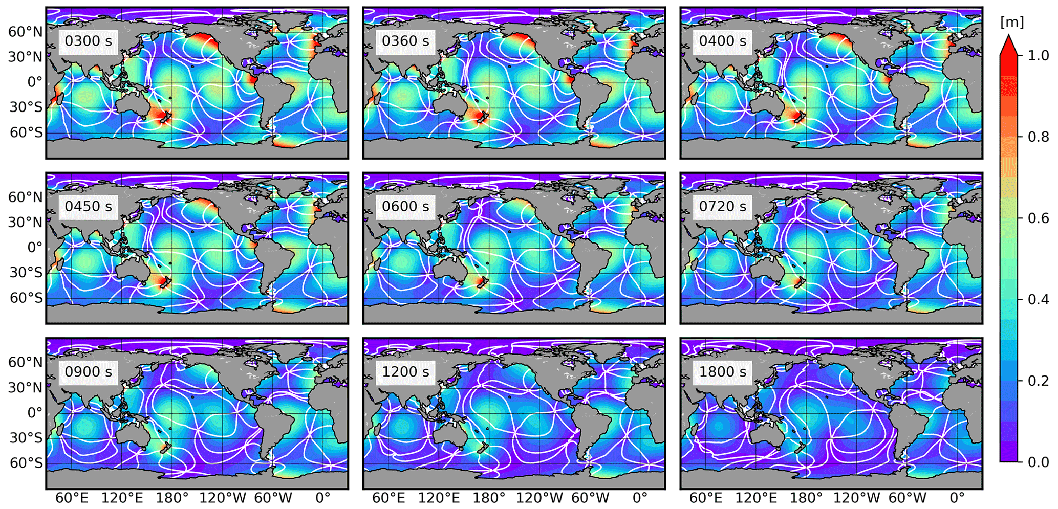
Figure A1Co-tidal charts of M2 tides from the time step sensitivity runs. The colours indicate tide amplitudes, and the white lines indicate Greenwich phase lags with an interval of 60∘. The time step setting in each run is labelled in each panel.
To quantitatively determine the time step for the best performance of the tidal potential module applying CORE-II mesh, we compare the harmonic tidal constants from the model results with those from tide gauge data. The University of Hawaii Sea Level Centre research quality data (Caldwell et al., 2015) are applied in this work. We obtain 687 tide gauge series at 540 tide gauge stations. Note that some tide gauge series refer to the same station, and we integrate those into one. We exclude some tide gauge stations because (1) these stations are not located in the CORE-II mesh, and (2) the water depths at these stations in the model are shallower than 200 m. We exclude shelf tide gauges because global tide models do not have a good performance in shelf areas inherently. Improving model results in shelf areas may lead to a larger error in the global view. A similar approach is also used in previous work that compares model results with pelagic tide gauges (Müller et al., 2010). Since most tide gauges span multiple years, each tide gauge series is truncated into several yearly segments according to the calendar year. For the preciseness of analysis, segments with a completeness index (proportion of data span without missing data) lower than 0.8 are discarded. Tidal harmonic analysis is done for each annual segment at each station, and the harmonic tidal constants at each station are thus averaged from multiyear constants. Finally, 229 tide gauge stations are applied for the comparison with model results.
A root-mean-square error (RMSE), referring to Cummins and Oey (1997), is defined as below to estimate the deviations of model results.
In Eq. (A1), Ao and ϕo represent tidal amplitudes and Greenwich phase lags derived from the observational data, while Am and ϕm represent those derived from the model results. It should be noted here that the RMSE defined in Eq. (A1) can be evaluated either for one tidal component throughout all tide gauges or several tidal components at one tide gauge. In the first case, N=229 for one tidal component throughout all 229 tide gauge stations (see Fig. A2a); in the second case, N=2 for two main diurnal/semidiurnal tidal components at one tide gauge station (see Fig. A2b and c). Figure A2a shows the RMSEs at all tide gauge stations for each sensitivity run's four main tidal constituents. It can be found that the last two sensitivity runs present significant errors for M2 tides. As we claim before in Fig. A1, a large time step may not resolve fast-travelling barotropic tides, leading to the damping of tide amplitudes. By considering all RMSEs of the four main tidal constituents, one can find that an optimal time step lies between 450 and 720 s. Considering the computational cost, we finally choose a time step of 720 s to simulate global tides with the CORE-II mesh. With the time step set to 720 s, the RMSEs for diurnal (O1 and K1) and semidiurnal (M2 and S2) tidal components at each tide gauge station are further shown in Fig. A2b and c, respectively. It can be seen that semidiurnal tides have larger deviations than diurnal ones, and gauges close to the coasts have larger deviations than those in basin centres.
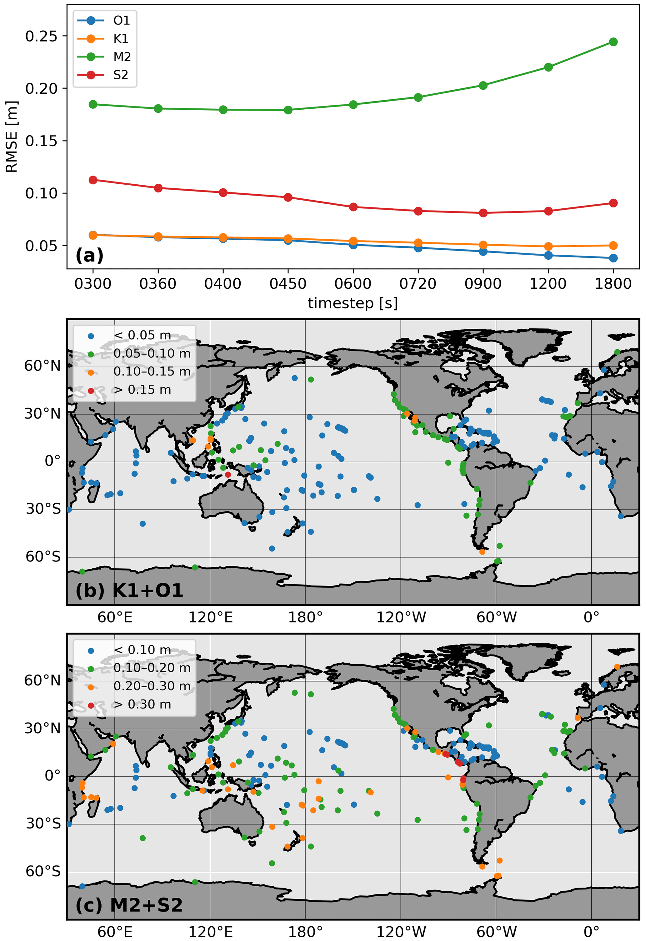
Figure A2(a) RMSE of the four main tidal components (O1, K1, M2 and S2 tides) for all 229 tide gauges. (b) In the sensitivity run with time step set to 720 s, RMSE of the main diurnal tidal components (O1 and K1 tides) at each tide-gauging station. Scatter points are classified into four levels by the magnitudes of RMSE. (c) The same as panel (b) but for the main semidiurnal tidal components (M2 and S2 tides).
In general, the tidal potential model demonstrates good consistency with tide gauges in most areas. However, we should state that some tide gauges also show considerable inconsistency from series to series and from year to year. For example, the Greenwich phase lags at some stations may have a discrepancy exceeding 120∘ among different years. That would introduce significant errors in estimating harmonic tidal constants at these stations. We speculate that the inconsistency may come from the changing of observational instruments.
B1 Calculation of the energy budget in FESOM2
We start from the ocean momentum balance Eq. (B1); uh and u are horizontal and three-dimensional velocity vectors; f is the Coriolis parameter; is the unit vector of the Earth angular velocity; ρ0 is a constant reference density; P represents the hydrostatic pressure; g is the gravitational acceleration; η is sea surface height; Ω is the tidal potential, which is also explained in Eq. (1); and Ah and Av are horizontal and vertical viscosity coefficients. ∇ and ∇h represent three-dimensional and horizontal gradient operators, respectively. Note here our experiment setting does not consider sea ice pressure and air pressure; thus, surface pressure only comes from the sea surface height.
The dot product between Eq. (B1) and ρ0uh gives Eq. (B2); ρ is seawater density minus the constant reference density ρ0, and ke means kinetic energy, which is expressed as .
A global, full-depth integration and long-term mean drop out some minor terms and give Eq. (B3). Note here that our experiment setting considers free slip lateral boundaries, so the integration of horizontal viscous term does not involve lateral friction. Nevertheless, the integration of vertical viscous term involves surface and bottom stress terms, in which us and ub are surface and bottom horizontal velocities, and τs and τb are surface and bottom stress.
In FESOM2, the horizontal viscosity is not calculated with an explicit form (Juricke et al., 2019). In order to evaluate the horizontal viscous dissipation, we have to directly compute the acceleration caused by horizontal viscosity (Gvisch) in the model. Thus the horizontal viscous dissipation term is actually calculated with uh⋅Gvisch. The kinetic energy budget in FESOM2 is finally given as Eq. (B4). Note here we introduce buoyancy into the first term of the right-hand side.
Thus, on the right-hand side of Eq. (B4), in order, we have the buoyancy flux term, the barotropic potential energy–kinetic energy conversion term, the tidal potential power term, the horizontal viscous dissipation term, the vertical viscous dissipation term, the wind stress term and the bottom friction term. Theoretically, in a global, full-depth integration and long-term mean, these terms should balance out. Residuals may come from (1) the integral of terms we omit from Eqs. (B2) to (B3), (2) horizontal interpolation between triangle vertices and triangle centroid or vertical interpolation between the cell surface and cell centre, and (3) the time difference between each term in Eq. (B1) and the velocity applied in the dot product. As for the third point, to reduce the residual term, we suggest using the central time velocity instead of the updated velocity at each model time step, especially for the velocity–sea surface height coupled term in a tidal case. In addition, all terms are calculated at each time step and then averaged over time (take buoyancy flux as an example, instead of ).
B2 The relationship between turbulent buoyancy flux and vertical diffusivity
Equation (B5) shows the ocean mass balance equation. Kh and Kv are horizontal and vertical diffusivity coefficients. S represents other source and sink terms regarding the mass balance. For the following derivation, we use buoyancy b instead of seawater density ρ here.
Splitting turbulence terms from the advection terms gives Eq. (B6), in which overlines denote the time mean, and primes denote turbulence.
A vertical advection–diffusion balance (e.g. Munk and Wunsch, 1998) gives Eq. (B7) below.
The vertical diffusivity parameter Kv represents the turbulent buoyancy fluxes that cannot be resolved in the model. In a traditional OGCM, such as NOTIDE/CVTIDE, the ocean currents roughly follow the geostrophic balance, but in LSTIDE we add ageostrophic flows. Tidal flows can easily cross the isobaths, therefore generating upwelling/downwelling around topographies, which alters turbulent buoyancy fluxes . Assuming tidal motion to be turbulence of the ocean mean flow, CVTIDE parameterises turbulent buoyancy fluxes by altering the vertical diffusivity parameter Kv. Thus, in Eq. (B7), CVTIDE mainly changes the second right-hand-side term, while LSTIDE mainly changes the first right-hand-side term. That is why LSTIDE shows stronger MOC without enhancing the vertical diffusivity in the model.
Note here we use to calculate turbulent buoyancy flux from the model results.
B3 Estimating internal tide scale in the model
With a given stratification, N2(z), one can first solve the mode-n eigenvector Φn(z) and the respective mode-n eigenvalue cn via the Sturm–Liouville equation below. In this work, we only study mode-1 internal tides.
With eigenvalue speeds cn, according to Falahat and Nycander (2015) and Song and Chen (2020), the wavenumbers kn of internal tides in the model are calculated as below.
In Eq. (B9), ω means the angular frequency of a tidal component, and f represents the Coriolis frequency, which changes with latitude. The first case of Eq. (B9) applies to propagating internal tides, occurring below the critical latitudes. The second case of Eq. (B9) applies to trapped internal tides, occurring beyond the critical latitudes. Note that even though trapped internal tides do not propagate, they are confined within a scale related to kn.
Finally, one can calculate the scale of an internal tide via .
The FESOM2.1 source code applied in this work, the last 50 years' averaged model results, and the postprocessing and visualisation codes are archived on Zenodo (https://doi.org/10.5281/zenodo.7457752, Song et al., 2021). The whole simulation results can be obtained by contacting the corresponding author. The tide gauge data (Caldwell et al., 2015) can be downloaded from the University of Hawaii Sea Level Centre's website (https://uhslc.soest.hawaii.edu/, last access: 27 July 2020, DOI: https://doi.org/10.7289/V5V40S7W). The PHC3 climatology (http://psc.apl.washington.edu/nonwp_projects/PHC/Climatology.html, Ermold and Steele, 2022; Steele et al., 2001), WOA18 climatology (https://www.ncei.noaa.gov/products/world-ocean-atlas, NCEI, 2022; Locarnini et al., 2019; Zweng et al., 2019) and CORE-II forcing (https://data1.gfdl.noaa.gov/nomads/forms/core/COREv2.html, Geophysical Fluid Dynamics Laboratory, 2022; Large and Yeager, 2009) are freely available online.
PeS and DS implemented the tidal module into FESOM2. PaS implemented the CVMIX package into FESOM2. PeS performed all the experiments. MT and GL contributed to the revision of the manuscript. All authors contributed to the analysis of the results.
The contact author has declared that none of the authors has any competing interests.
Publisher’s note: Copernicus Publications remains neutral with regard to jurisdictional claims in published maps and institutional affiliations.
The authors thank Nikolay Koldunov for the help with FESOM2 settings and Sergey Danilov for discussing the model results. Pengyang Song is funded by the China Scholarship Council (grant no. 201906330073). Gerrit Lohmann and Maik Thomas received funding through the topic “Ocean and Cryosphere under climate change” in the programme “Changing Earth – Sustaining our Future”. The experiments were performed at the AWI Computing Centre.
This research has been supported by the China Scholarship Council (grant no. 201906330073). Gerrit Lohmann and Maik Thomas received funding through the Helmholtz programme “Changing Earth – Sustaining our Future”.
The article processing charges for this open-access publication were covered by the Alfred Wegener Institute, Helmholtz Centre for Polar and Marine Research (AWI).
This paper was edited by Riccardo Farneti and reviewed by Jonas Nycander and two anonymous referees.
Accad, Y. and Pekeris, C. L.: Solution of the tidal equations for the M2 and S2 tides in the world oceans from a knowledge of the tidal potential alone, Philos. T. R. Soc. S.-A, 290, 235–266, https://doi.org/10.1098/rsta.1978.0083, 1978. a
Ackermann, L., Danek, C., Gierz, P., and Lohmann, G.: AMOC Recovery in a Multicentennial Scenario Using a Coupled Atmosphere-Ocean-Ice Sheet Model, Geophys. Res. Lett., 47, e2019GL086810, https://doi.org/10.1029/2019GL086810, 2020. a
Arbic, B. K., Alford, M. H., Ansong, J. K., Buijsman, M. C., Ciotti, R. B., Farrar, J. T., Hallberg, R. W., Henze, C. E., Hill, C. N., Luecke, C. A., Menemenlis, D., Metzger, E. J., Müeller, M., Nelson, A. D., Nelson, B. C., Ngodock, H. E., Ponte, R. M., Richman, J. G., Savage, A. C., Scott, R. B., Shriver, J. F., Simmons, H. L., Souopgui, I., Timko, P. G., Wallcraft, A. J., Zamudio, L., and Zhao, Z.: A Primer on Global Internal Tide and Internal Gravity Wave Continuum Modeling in HYCOM and MITgcm, in: New Frontiers in Operational Oceanography, GODAE OceanView, 307–392, https://doi.org/10.17125/gov2018.ch13, 2018. a
Bessières, L., Madec, G., and Lyard, F.: Global tidal residual mean circulation: Does it affect a climate OGCM?, Geophys. Res. Lett., 35, L03609, https://doi.org/10.1029/2007GL032644, 2008. a
Biastoch, A., Böning, C. W., and Lutjeharms, J.: Agulhas leakage dynamics affects decadal variability in Atlantic overturning circulation, Nature, 456, 489–492, https://doi.org/10.1038/nature07426, 2008. a
Bryan, F.: Parameter Sensitivity of Primitive Equation Ocean General Circulation Models, J. Phys. Oceanogr., 17, 970–985, https://doi.org/10.1175/1520-0485(1987)017<0970:PSOPEO>2.0.CO;2, 1987. a
Caldwell, P. C., Merrifield, M. A., and Thompson, P. R.: Sea level measured by tide gauges from global oceans as part of the Joint Archive for Sea Level (JASL) since 1846, NOAA National Centers for Environmental Information [data set], https://doi.org/10.7289/V5V40S7W, 2015. a, b
Cummins, P. F. and Oey, L. Y.: Simulation of barotropic and baroclinic tides off northern British Columbia, J. Phys. Oceanogr., 27, 762–781, https://doi.org/10.1175/1520-0485(1997)027<0762:SOBABT>2.0.CO;2, 1997. a
Danek, C., Scholz, P., and Lohmann, G.: Effects of high resolution and spinup time on modeled North Atlantic circulation, J. Phys. Oceanogr., 49, 1159–1181, https://doi.org/10.1175/JPO-D-18-0141.1, 2019. a
Danilov, S., Sidorenko, D., Wang, Q., and Jung, T.: The Finite-volumE Sea ice–Ocean Model (FESOM2), Geosci. Model Dev., 10, 765–789, https://doi.org/10.5194/gmd-10-765-2017, 2017. a, b, c
Duffett-Smith, P.: Astronomy with your Personal Computer, 2 edn., Cambridge University Press, https://doi.org/10.1017/CBO9780511564888, 1990. a
Ermold, W. and Steele, M.: Polar science center Hydrographic Climatology (PHC), Polar Science Center [data set], http://psc.apl.washington.edu/nonwp_projects/PHC/Climatology.html, last access: 11 August 2022. a
Exarchou, E., Von Storch, J. S., and Jungclaus, J. H.: Impact of tidal mixing with different scales of bottom roughness on the general circulation, Ocean Dynam., 62, 1545–1563, https://doi.org/10.1007/s10236-012-0573-1, 2012. a
Falahat, S. and Nycander, J.: On the generation of bottom-trapped internal tides, J. Phys. Oceanogr., 45, 526–545, https://doi.org/10.1175/JPO-D-14-0081.1, 2015. a, b
Ferrari, R., Griffies, S. M., Nurser, A. G., and Vallis, G. K.: A boundary-value problem for the parameterized mesoscale eddy transport, Ocean Model., 32, 143–156, https://doi.org/10.1016/j.ocemod.2010.01.004, 2010. a
Ferrari, R., Mashayek, A., McDougall, T. J., Nikurashin, M., and Campin, J. M.: Turning ocean mixing upside down, J. Phys. Oceanogr., 46, 2239–2261, https://doi.org/10.1175/JPO-D-15-0244.1, 2016. a
Friedrich, T., Timmermann, A., Decloedt, T., Luther, D. S., and Mouchet, A.: The effect of topography-enhanced diapycnal mixing on ocean and atmospheric circulation and marine biogeochemistry, Ocean Model., 39, 262–274, https://doi.org/10.1016/j.ocemod.2011.04.012, 2011. a, b
Gent, P. R. and Mcwilliams, J. C.: Isopycnal Mixing in Ocean Circulation Models, J. Phys. Oceanogr., 20, 150–155, https://doi.org/10.1175/1520-0485(1990)020<0150:imiocm>2.0.co;2, 1990. a, b
Geophysical Fluid Dynamics Laboratory: Version 2 Forcing for Coordinated Ocean-ice Reference Experiments (CORE), Geophysical Fluid Dynamics Laboratory [data set], https://data1.gfdl.noaa.gov/nomads/forms/core/COREv2.html, last access: 11 August 2022. a
Griffies, S. M., Levy, M., Adcroft, A. J., Danabasoglu, G., Hallberg, R. W., Jacobsen, D., Large, W., and Ringler, T.: Theory and numerics of the Community Ocean Vertical Mixing (CVMix) project, Technical Report, https://github.com/CVMix/CVMix-description/blob/master/cvmix.pdf (last access: 9 January 2022), 2015. a
Hibler, W. D.: A Dynamic Thermodynamic Sea Ice Model, J. Phys. Oceanogr., 9, 815–846, https://doi.org/10.1175/1520-0485(1979)009<0815:ADTSIM>2.0.CO;2, 1979. a
Huang, R. X.: Energetics of the oceanic circulation, in: Ocean Circulation: Wind-Driven and Thermohaline Processes, Cambridge University Press, Cambridge, 149–258, https://doi.org/10.1017/CBO9780511812293.004, 2009. a
Itoh, S., Tanaka, Y., Osafune, S., Yasuda, I., Yagi, M., Kaneko, H., Konda, S., Nishioka, J., and N. Volkov, Y.: Direct breaking of large-amplitude internal waves in the Urup Strait, Prog. Oceanogr., 126, 109–120, https://doi.org/10.1016/j.pocean.2014.04.014, 2014. a
Jayne, S. R.: The impact of abyssal mixing parameterizations in an ocean general circulation model, J. Phys. Oceanogr., 39, 1756–1775, https://doi.org/10.1175/2009JPO4085.1, 2009. a, b, c
Jayne, S. R. and St. Laurent, L. C.: Parameterizing tidal dissipation over rough topography, Geophys. Res. Lett., 28, 811–814, https://doi.org/10.1029/2000GL012044, 2001. a
Juricke, S., Danilov, S., Kutsenko, A., and Oliver, M.: Ocean kinetic energy backscatter parametrizations on unstructured grids: Impact on mesoscale turbulence in a channel, Ocean Model., 138, 51–67, https://doi.org/10.1016/j.ocemod.2019.03.009, 2019. a, b
Kantha, L. H.: Barotropic tides in the global oceans from a nonlinear tidal model assimilating altimetric tides 1. Model description and results, J. Geophys. Res., 100, 25283–25308, https://doi.org/10.1029/95jc02578, 1995. a
Koch-Larrouy, A., Madec, G., Bouruet-Aubertot, P., Gerkema, T., Bessières, L., and Molcard, R.: On the transformation of Pacific Water into Indonesian Throughflow Water by internal tidal mixing, Geophys. Res. Lett., 34, L04604, https://doi.org/10.1029/2006GL028405, 2007. a
Large, W. G. and Yeager, S. G.: The global climatology of an interannually varying air–sea flux data set, Clim. Dynam., 33, 341–364, https://doi.org/10.1007/s00382-008-0441-3, 2009. a, b
Large, W. G., McWilliams, J. C., and Doney, S. C.: Oceanic vertical mixing: A review and a model with a nonlocal boundary layer parameterization, Rev. Geophys., 32, 363–403, https://doi.org/10.1029/94RG01872, 1994. a
Ledwell, J. R., Montgomery, E. T., Polzin, K. L., St. Laurent, L. C., Schmitt, R. W., and Toole, J. M.: Evidence for enhanced mixing over rough topography in the abyssal ocean, Nature, 403, 179–182, https://doi.org/10.1038/35003164, 2000. a, b, c
Lee, H. C., Rosati, A., and Spelman, M. J.: Barotropic tidal mixing effects in a coupled climate model: Oceanic conditions in the Northern Atlantic, Ocean Model., 11, 464–477, https://doi.org/10.1016/j.ocemod.2005.03.003, 2006. a, b
Lemarié, F., Debreu, L., Madec, G., Demange, J., Molines, J. M., and Honnorat, M.: Stability constraints for oceanic numerical models: Implications for the formulation of time and space discretizations, Ocean Model., 92, 124–148, https://doi.org/10.1016/j.ocemod.2015.06.006, 2015. a
Li, Z., von Storch, J. S., and Müller, M.: The M2 internal tide simulated by a ∘ OGCM, J. Phys. Oceanogr., 45, 3119–3135, https://doi.org/10.1175/JPO-D-14-0228.1, 2015. a
Locarnini, R. A., Mishonov, A.V., Baranova, O. K., Boyer, T. P., Zweng, M. M., Garcia, H. E., Reagan, J. R., Seidov, D., Weathers, K. W., Paver, C. R., and Smolyar, I. V.: World Ocean Atlas 2018 Volume 1: Temperature, edited by: Mishonov, A., Technical Editor, NOAA Atlas NESDIS, 81, 52 pp., 2019. a, b
Logemann, K., Linardakis, L., Korn, P., and Schrum, C.: Global tide simulations with ICON-O: testing the model performance on highly irregular meshes, Ocean Dynam., 71, 43–57, https://doi.org/10.1007/s10236-020-01428-7, 2021. a
Lohmann, G.: Temperatures from energy balance models: the effective heat capacity matters, Earth Syst. Dynam., 11, 1195–1208, https://doi.org/10.5194/esd-11-1195-2020, 2020. a
Lohmann, G., Butzin, M., Eissner, N., Shi, X., and Stepanek, C.: Abrupt Climate and Weather Changes Across Time Scales, Paleoceanography and Paleoclimatology, 35, e2019PA003782, https://doi.org/10.1029/2019PA003782, 2020. a
Marshall, J. and Speer, K.: Closure of the meridional overturning circulation through Southern Ocean upwelling, Nat. Geosci., 5, 171–180, https://doi.org/10.1038/ngeo1391, 2012. a
Melet, A., Legg, S., and Hallberg, R.: Climatic impacts of parameterized local and remote tidal mixing, J. Climate, 29, 3473–3500, https://doi.org/10.1175/JCLI-D-15-0153.1, 2016. a
Müller, M., Haak, H., Jungclaus, J. H., Sündermann, J., and Thomas, M.: The effect of ocean tides on a climate model simulation, Ocean Model., 35, 304–313, https://doi.org/10.1016/j.ocemod.2010.09.001, 2010. a, b, c
Munk, W. and Wunsch, C.: Abyssal recipes II: Energetics of tidal and wind mixing, Deep-Sea Res. Pt. I, 45, 1977–2010, https://doi.org/10.1016/S0967-0637(98)00070-3, 1998. a, b, c, d, e, f
Nagai, T. and Hibiya, T.: Internal tides and associated vertical mixing in the Indonesian Archipelago, J. Geophys. Res.-Oceans, 120, 3373–3390, https://doi.org/10.1002/2014JC010592, 2015. a
Nakamura, T., Isoda, Y., Mitsudera, H., Takagi, S., and Nagasawa, M.: Breaking of unsteady lee waves generated by diurnal tides, Geophys. Res. Lett., 37, L04602, https://doi.org/10.1029/2009GL041456, 2010. a
National Centers for Environmental Information (NCEI): World Ocean Atlas, NCEI [data set], https://www.ncei.noaa.gov/products/world-ocean-atlas, last access: 11 August 2022. a
Niwa, Y. and Hibiya, T.: Estimation of baroclinic tide energy available for deep ocean mixing based on three-dimensional global numerical simulations, J. Oceanogr., 67, 493–502, https://doi.org/10.1007/s10872-011-0052-1, 2011. a, b
Niwa, Y. and Hibiya, T.: Generation of baroclinic tide energy in a global three-dimensional numerical model with different spatial grid resolutions, Ocean Model., 80, 59–73, https://doi.org/10.1016/j.ocemod.2014.05.003, 2014. a, b
Oka, A. and Niwa, Y.: Pacific deep circulation and ventilation controlled by tidal mixing away from the sea bottom, Nat. Commun., 4, 2419, https://doi.org/10.1038/ncomms3419, 2013. a, b
Olbers, D. and Eden, C.: A global model for the diapycnal diffusivity induced by internal gravity waves, J. Phys. Oceanogr., 43, 1759–1779, https://doi.org/10.1175/JPO-D-12-0207.1, 2013. a
Osborn, T. R.: Estimates of the Local Rate of Vertical Diffusion from Dissipation Measurements, J. Phys. Oceanogr., 10, 83–89, https://doi.org/10.1175/1520-0485(1980)010<0083:EOTLRO>2.0.CO;2, 1980. a
Pawlowicz, R., Beardsley, B., and Lentz, S.: Classical tidal harmonic analysis including error estimates in MATLAB using TDE, Comput. Geosci., 28, 929–937, https://doi.org/10.1016/S0098-3004(02)00013-4, 2002. a
Polzin, K. L., Toole, J. M., Ledwell, J. R., and Schmitt, R. W.: Spatial variability of turbulent mixing in the abyssal ocean, Science, 276, 93–96, https://doi.org/10.1126/science.276.5309.93, 1997. a, b, c, d
Prange, M., Lohmann, G., and Paul, A.: Influence of Vertical Mixing on the Thermohaline Hysteresis: Analyses of an OGCM, J. Phys. Oceanogr., 33, 1707–1721, https://doi.org/10.1175/1520-0485(2003)033<1707:iovmot>2.0.co;2, 2003. a
Ray, R. D.: Ocean self-attraction and loading in numerical tidal models, Mar. Geod., 21, 181–192, https://doi.org/10.1080/01490419809388134, 1998. a
Redi, M. H.: Oceanic isopycnal mixing by coordinate rotation, J. Phys. Oceanogr., 12, 1154–1158, https://doi.org/10.1175/1520-0485(1982)012<1154:OIMBCR>2.0.CO;2, 1982. a
Saenko, O. A. and Merryfield, W. J.: On the effect of topographically enhanced mixing on the global ocean circulation, J. Phys. Oceanogr., 35, 826–834, https://doi.org/10.1175/JPO2722.1, 2005. a, b
Sasaki, H., Kida, S., Furue, R., Nonaka, M., and Masumoto, Y.: An Increase of the Indonesian Throughflow by Internal Tidal Mixing in a High-Resolution Quasi-Global Ocean Simulation, Geophys. Res. Lett., 45, 8416–8424, https://doi.org/10.1029/2018GL078040, 2018. a
Schiller, A.: Effects of explicit tidal forcing in an OGCM on the water-mass structure and circulation in the Indonesian throughflow region, Ocean Model., 6, 31–49, https://doi.org/10.1016/S1463-5003(02)00057-4, 2004. a, b
Scholz, P., Sidorenko, D., Gurses, O., Danilov, S., Koldunov, N., Wang, Q., Sein, D., Smolentseva, M., Rakowsky, N., and Jung, T.: Assessment of the Finite-volumE Sea ice-Ocean Model (FESOM2.0) – Part 1: Description of selected key model elements and comparison to its predecessor version, Geosci. Model Dev., 12, 4875–4899, https://doi.org/10.5194/gmd-12-4875-2019, 2019. a
Scholz, P., Sidorenko, D., Danilov, S., Wang, Q., Koldunov, N., Sein, D., and Jung, T.: Assessment of the Finite-VolumE Sea ice–Ocean Model (FESOM2.0) – Part 2: Partial bottom cells, embedded sea ice and vertical mixing library CVMix, Geosci. Model Dev., 15, 335–363, https://doi.org/10.5194/gmd-15-335-2022, 2022. a
Scott, J. R. and Marotzke, J.: The Location of Diapycnal Mixing and the Meridional Overturning Circulation, J. Phys. Oceanogr., 32, 3578–3595, https://doi.org/10.1175/1520-0485(2002)032<3578:TLODMA>2.0.CO;2, 2002. a
Shchepetkin, A. F.: An adaptive, Courant-number-dependent implicit scheme for vertical advection in oceanic modeling, Ocean Model., 91, 38–69, https://doi.org/10.1016/j.ocemod.2015.03.006, 2015. a
Shi, X. and Lohmann, G.: Simulated response of the mid-Holocene Atlantic meridional overturning circulation in ECHAM6-FESOM/MPIOM, J. Geophys. Res.-Oceans, 121, 6444–6469, https://doi.org/10.1002/2015JC011584, 2016. a
Shihora, L., Sulzbach, R., Dobslaw, H., and Thomas, M.: Self-attraction and loading feedback on ocean dynamics in both shallow water equations and primitive equations, Ocean Model., 169, 101914, https://doi.org/10.1016/j.ocemod.2021.101914, 2022. a
Shriver, J. F., Arbic, B. K., Richman, J. G., Ray, R. D., Metzger, E. J., Wallcraft, A. J., and Timko, P. G.: An evaluation of the barotropic and internal tides in a high-resolution global ocean circulation model, J. Geophys. Res.-Oceans, 117, C10024, https://doi.org/10.1029/2012JC008170, 2012. a, b
Sidorenko, D., Danilov, S., Koldunov, N., Scholz, P., and Wang, Q.: Simple algorithms to compute meridional overturning and barotropic streamfunctions on unstructured meshes, Geosci. Model Dev., 13, 3337–3345, https://doi.org/10.5194/gmd-13-3337-2020, 2020. a, b, c
Simmons, H. L., Jayne, S. R., St. Laurent, L. C., and Weaver, A. J.: Tidally driven mixing in a numerical model of the ocean general circulation, Ocean Model., 6, 245–263, https://doi.org/10.1016/S1463-5003(03)00011-8, 2004. a, b, c, d
Song, P. and Chen, X.: Investigation of the Internal Tides in the Northwest Pacific Ocean Considering the Background Circulation and Stratification, J. Phys. Oceanogr., 50, 3165–3188, https://doi.org/10.1175/JPO-D-19-0177.1, 2020. a
Song, P., Sidorenko, D., Scholz, P., Thomas, M., and Lohmann, G.: The tidal effects in the Finite-volumE Sea ice–Ocean Model (FESOM2.1): a comparison between parameterized tidal mixing and explicit tidal forcing, Zenodo [code and data set], https://doi.org/10.5281/zenodo.7457752, 2021. a
Steele, M., Morley, R., and Ermold, W.: PHC: A Global Ocean Hydrography with a High-Quality Arctic Ocean, J. Climate, 14, 2079–2087, https://doi.org/10.1175/1520-0442(2001)014<2079:PAGOHW>2.0.CO;2, 2001. a, b
Stepanov, V. N. and Hughes, C. W.: Parameterization of ocean self-attraction and loading in numerical models of the ocean circulation, J. Geophys. Res.-Oceans, 109, C03037, https://doi.org/10.1029/2003jc002034, 2004. a
St. Laurent, L. C., Simmons, H. L., and Jayne, S. R.: Estimating tidally driven mixing in the deep ocean, Geophys. Res. Lett., 29, 2106, https://doi.org/10.1029/2002GL015633, 2002. a
Sulzbach, R., Dobslaw, H., and Thomas, M.: High-Resolution Numerical Modeling of Barotropic Global Ocean Tides for Satellite Gravimetry, J. Geophys. Res.-Oceans, 126, e2020JC017097, https://doi.org/10.1029/2020JC017097, 2021. a
Talley, L. D., Pickard, G. L., Emery, W. J., and Swift, J. H.: Chapter S14 – Global Circulation and Water Properties: Supplementary Materials, in: Descriptive Physical Oceanography (Sixth Edition), 6 edn., Academic Press, Boston, 1–9, https://doi.org/10.1016/B978-0-7506-4552-2.10026-5, 2011. a
Tanaka, T., Yasuda, I., Tanaka, Y., and Carter, G. S.: Numerical study on tidal mixing along the shelf break in the Green Belt in the southeastern Bering Sea, J. Geophys. Res.-Oceans, 118, 6525–6542, https://doi.org/10.1002/2013JC009113, 2013. a
Tanaka, Y., Hibiya, T., Niwa, Y., and Iwamae, N.: Numerical study of K1 internal tides in the Kuril straits, J. Geophys. Res.-Oceans, 115, C09016, https://doi.org/10.1029/2009JC005903, 2010. a
Tatebe, H., Tanaka, Y., Komuro, Y., and Hasumi, H.: Impact of deep ocean mixing on the climatic mean state in the Southern Ocean, Scientific Reports, 8, 14479, https://doi.org/10.1038/s41598-018-32768-6, 2018. a, b
Thomas, M., Sündermann, J., and Maier-Reimer, E.: Consideration of ocean tides in an OGCM and impacts on subseasonal to decadal polar motion excitation, Geophys. Res. Lett., 28, 2457–2460, https://doi.org/10.1029/2000GL012234, 2001. a, b
Tsujino, H., Hasumi, H., and Suginohara, N.: Deep Pacific Circulation Controlled by Vertical Diffusivity at the Lower Thermocline Depths, J. Phys. Oceanogr., 30, 2853–2865, https://doi.org/10.1175/1520-0485(2001)031<2853:DPCCBV>2.0.CO;2, 2000. a
Wahr, J. M.: Body tides on an elliptical, rotating, elastic and oceanless earth, Geophys. J. Int., 64, 677–703, https://doi.org/10.1111/j.1365-246X.1981.tb02690.x, 1981. a
Wang, Q., Danilov, S., Sidorenko, D., Timmermann, R., Wekerle, C., Wang, X., Jung, T., and Schröter, J.: The Finite Element Sea Ice-Ocean Model (FESOM) v.1.4: formulation of an ocean general circulation model, Geosci. Model Dev., 7, 663–693, https://doi.org/10.5194/gmd-7-663-2014, 2014. a
Weber, T. and Thomas, M.: Tidal dynamics and their influence on the climate system from the Cretaceous to present day, Global Planet. Change, 158, 173–183, https://doi.org/10.1016/j.gloplacha.2017.09.019, 2017. a
Yu, Y., Liu, H., and Lan, J.: The influence of explicit tidal forcing in a climate ocean circulation model, Acta Oceanol. Sin., 35, 42–50, https://doi.org/10.1007/s13131-016-0931-9, 2016. a, b
Zweng, M. M., Reagan, J. R., Seidov, D., Boyer T. P., Locarnini, R. A., Garcia, H. E., Mishonov, A. V., Baranova, O. K., Weathers, K. W., Paver, C. R., and Smolyar, I. V.: World Ocean Atlas 2018, Volume 2: Salinity, edited by: Mishonov, A., Technical Editor, NOAA Atlas NESDIS, 82, 50 pp., 2019. a, b
- Abstract
- Introduction
- Model description
- Model results
- Discussion
- Conclusions
- Appendix A: Validation of the tidal potential module
- Appendix B: Theoretical background and equation derivation
- Code and data availability
- Author contributions
- Competing interests
- Disclaimer
- Acknowledgements
- Financial support
- Review statement
- References