Deep learning for stochastic precipitation generation – deep SPG v1.0

We present a deep-neural-network-based single-site stochastic precipitation generator (SPG), capable of producing realistic time series of daily and hourly precipitation. The neural network outputs a wet-day probability and precipitation distributions in the form of a mixture model. The SPG was tested in four different locations in New Zealand, and we found it accurately reproduced the precipitation depth, the autocorrelations seen in the original data, the observed dry-spell lengths, and the seasonality in precipitation. We present two versions of the hourly and daily SPGs: (i) a stationary version of the SPG that assumes that the statistics of the precipitation are time independent and (ii) a non-stationary version that captures the secular drift in precipitation statistics resulting from climate change. The latter was developed to be applicable to climate change impact studies, especially studies reliant on SPG projections of future precipitation. We highlight many of the pitfalls associated with the training of a non-stationary SPG on observations alone and offer an alternative method that replicates the secular drift in precipitation seen in a large-ensemble regional climate model. The SPG runs several orders of magnitude faster than a typical regional climate model and permits the generation of very large ensembles of realistic precipitation time series under many climate change scenarios. These ensembles will also contain many extreme events not seen in the historical record.

1 Introduction

The effects of climate change are often most acutely felt in the form of changes in the severity, or in frequency, of extreme precipitation events (EPEs) (van der Wiel and Bintanja, 2021; Li et al., 2021; Lewis et al., 2019).

Modelling expected changes in EPEs is challenging. They often occur on spatial scales of several kilometres, an order of magnitude smaller than the spatial scales simulated by regional climate models (RCMs), and perhaps 2 orders of magnitude smaller than the scales typically simulated by global climate models (GCMs; Wedi et al., 2020). Furthermore, EPEs are, by definition, rare. As a result, modelling expected changes in the frequency and severity of EPEs requires dynamical downscaling of GCMs, as well as the generation of very large ensembles of simulations. State-of-the-art GCMs are needed to correctly simulate expected changes in the dynamics underlying the synoptic conditions that lead to EPEs (Fahad et al., 2020b, a), while dynamical downscaling (Monjo et al., 2016; Castellano and DeGaetano, 2016), using an RCM, is required to capture scales typical of EPEs. Very large ensembles (hundreds of members) of simulations are required to allow sufficiently large populations of EPEs to derive robust statistics of expected changes in their frequency and their severity. Achieving these two requirements, at sufficiently high resolution, is prohibitively computationally expensive using currently available GCMs and RCMs.

Stochastic precipitation generators (SPGs) (Ahn, 2020; Iizumi et al., 2012; Wilks, 2010) can be designed and trained to emulate the precipitation at one or more sites simulated by GCMs containing nested regional climate models (RCMs). SPGs provide less computationally demanding approaches to generating the large ensembles of simulations required to adequately represent the statistics of EPEs.

SPGs can be trained on historical observations of daily or hourly precipitation to learn the statistical characteristics of the precipitation at that site. However, if the intent is to develop a non-stationary SPG – one capable of capturing climate-induced secular changes in the statistical nature of the precipitation – extracting this climate signal from historical precipitation records is itself challenging. Inhomogeneities in those records (Venema et al., 2012; Toreti et al., 2012; Peterson et al., 1998) resulting from, for example, changes in instrumentation can hide the underling climate-induced signal. Further, a rather weak climate signal in the past makes it difficult to learn the strong signal expected in the future. To avoid these challenges of measurement series inhomogeneity and the brevity of historical records, an alternative is to train the SPG on RCM simulations of past and future precipitation. However, GCMs and their nested RCMs have well-identified shortcomings in the simulation of precipitation (Li et al., 2014; Haerter et al., 2015; Piani et al., 2010). As such, without careful bias correction, the SPG would learn from biased RCM data, and therefore its simulations would be biased and it would not produce a realistic precipitation distribution.

As alluded to above, the statistics of precipitation, and in particular the statistics of EPEs, are expected to evolve under climate change. Developing an SPG architecture that is capable of capturing that non-stationarity, but avoids errant behaviour when applied outside the limits of the training data, is a particular challenge. These and other methodological choices have been explored in the construction of the SPGs described in this paper.

SPGs are a subset of the broader class of stochastic weather generators (SWGs) and, as with SWGs, they come in two broad types: parametric and non-parametric. Non-parametric SWGs simply resample the data, while parametric generators fit distributions to the data (Ailliot et al., 2015) and then use these distributions to create events outside the range of the training data. Therefore, while non-parametric SWGs cannot create an entirely new event outside of their training data, they can generate a unique sequence of such events.

Typically, parametric SWGs and SPGs simulate precipitation in two stages. The first stage decides whether precipitation occurs, while the second stage models the precipitation amount (Richardson, 1981). The material presented here focuses entirely on precipitation and follows from the class of SWGs first introduced by Katz (1977), where a gamma distribution was used to describe the precipitation amount. Because a single distribution is often insufficient to fully capture precipitation extremes, a mixture of different distributions was adopted in Carreau and Vrac (2011), who introduced a conditional mixture model for precipitation downscaling. Imperatives for the work presented herein were to build an SPG that learns the nature of the statistics of precipitation from observations alone (and is therefore not subject to the biases of GCMs or RCMs in training), including the inference of non-stationarity in the signal, and which only resorts to auxiliary model simulations where the observation record is found to be inadequate to capture the non-stationarity. An additional imperative was to have the non-stationarity described by a single annual mean hemispheric covariate time series that can be quickly and robustly simulated by a simple climate model for a wide range of future greenhouse gas emission scenarios. This makes the SPGs reported on below easily applicable to a wide range of climate impact studies that benefit from very large ensembles of precipitation projections.

2 Data

The following data sets were used for training, validating, or transforming the SPGs presented below. Both daily resolution and hourly resolution SPGs are presented here. Daily SPGs benefit from the availability of longer measurement series being available for their training as, prior to the development of automatic weather stations, precipitation data were typically recorded once each day. However, for many applications, especially for highly damaging extreme precipitation events, the distribution of precipitation over the course of a day can be important to resolve. As such, hourly resolution SPGs can have wider utility than daily SPGs. They suffer, however, from a paucity of data for their training. The benefits of the SPGs at both daily and hourly resolution are presented below.

2.1 Daily precipitation observations

Daily weather station precipitation data were obtained from CLIDB, NIWA's National Climate Database (https://cliflo.niwa.co.nz/, last access: 4 July 2023) for four cities in New Zealand: Auckland, Tauranga, Christchurch, and Dunedin. Each data point was the cumulative amount of precipitation measured each day. These four locations were selected as they represented a range of climatic regimes around New Zealand and are large population centres. The selected locations also had time series of hourly and daily precipitation data sufficiently long to achieve robust training.

In some cases, data from two weather stations were combined in order to generate records of longer duration. When combining data from two sites, the secondary site's data were used only where data were not available from the primary site. CLIDB details for the six stations used for daily data are listed in Table 1. Table 2 provides key statistics describing the data, after combination, for the four cities.

Table 1 Stations providing daily observations of precipitation. Where more than one station was used to construct the historical record for the location, the stations appear in priority order.

Additional data points were dropped if the data point's features (see Sect. 3.1.1) could not be calculated, due to the features requiring precipitation measurements from days with missing data. This treatment of missing data was required to ensure that the neural network (see Sect. 3) saw only valid data. Specifically, this meant that for 1 d of missing data we would drop the following 8 d, and thus the effective percentage of missing data was greater than the percentage missing in the source observation time series.

Table 2 Key attributes of the combined time series of daily precipitation observations.

2.2 Hourly precipitation observations

Hourly weather station precipitation data for the same four cities were obtained from CLIDB (see Table 3). Each data point was the cumulative amount of precipitation seen in the hour before the timestamp.

Table 3 Stations providing hourly observations of precipitation. Where more than one station was used to construct the historical record for the location, the stations appear in priority order.

Additional data points were dropped if the data point's features (see Sect. 3.1.2) could not be calculated, due to the features requiring precipitation measurements from hours with missing data. Specifically, this meant that for 1 h of missing data we would drop the 144 following hours, and thus the effective amount of missing data was greater than the amount missing in the source observation time series. Table 4 lists the volume of effective missing hourly data for the four locations.

Table 4 Key attributes of the combined time series of hourly precipitation observations.

2.3 Global-scale temperature anomalies

To describe the non-stationarity in the precipitation time series at each location, we sought a climate change covariate that would not be subject to small-scale temporal and spatial variability, would be easy to calculate for a range of greenhouse gas emission scenarios, and would be broadly applicable. We settled on the annual mean Southern Hemisphere mean surface temperature over land anomaly (hereafter $T_{\mathrm{SH}-\mathrm{land}}^{\prime }$). Time series of $T_{\mathrm{SH}-\mathrm{land}}^{\prime }$ for a range of different Representative Concentration Pathway (RCP) and Shared Socioeconomic Pathway (SSP) greenhouse gas emissions scenarios were obtained from the MAGICC simple climate model (Meinshausen et al., 2009, 2011, 2020). These annual time series extended from 1765 to 2150 and are anomalies with respect to 1765.

MAGICC is a probabilistic reduced complexity model, which was used to produce hemispherical land and ocean surface temperature time series for selected Shared Socioeconomic Pathways (SSPs Riahi et al., 2017). MAGICC version 7.5.1 simulations were constrained using a set of historical assessed ranges representative of the IPCC AR5 assessment with some additional updates (Nicholls et al., 2021) as part of the Reduced Complexity Model Intercomparison Project, RCMIP. A similar generation of MAGICC7 was used in various other studies, including IPCC AR6 WG1 and WG3 to assess the warming for a given pathway of emissions or concentrations (Meinshausen et al., 2022). From a-600 member MAGICC ensemble, the ensemble member with the median equilibrium climate sensitivity was used in this study, rather than calculating percentiles across the ensemble. This was done to ensure that the results were internally consistent – such that the hemispherical mean annual mean surface temperatures were consistent with global mean annual mean surface temperatures.

We use $T_{\mathrm{Global}}^{\prime }$ and $T_{\mathrm{SH}-\mathrm{land}}^{\prime }$ in Sects. 5 and 2.4.

2.4 Regional climate model precipitation simulations

While RCM simulations cannot generate precipitation time series that are unbiased with respect to historical observations and are seldom available at an hourly resolution, they do provide a means of quantifying the non-stationarity in precipitation, especially if observational records are too short to reliably extract the secular climate signal. These RCM simulations can provide a useful validation standard for a non-stationary SPG. To this end we obtained RCM simulations for the New Zealand region from the weather@home project (Massey et al., 2015; Black et al., 2016; Rosier et al., 2015). The weather@home project provides ensembles with many thousands of members, permitting the calculation of statistics with a high degree of confidence, even in the extremes. The resolution of these weather@home simulations was 0.44^∘, and the closest land-based grid cell was selected for each of the stations. Selecting a single weather@home grid cell may not be best practice when using the precipitation data directly as single grid cells may not be representative of the location due to, for example, inadequately resolved topography or due to the inability of a climate model to represent weather at this scale. In this study, however, the raw precipitation data are not used but rather the sensitivities of precipitation to a climate covariate (in this case $T_{\mathrm{SH}-\mathrm{land}}^{\prime }$); the field of such sensitivities is expected to be less spatially variable than the precipitation field itself. Whether a single cell or several neighbouring cells should be used to best quantify the sensitivity of precipitation to $T_{\mathrm{SH}-\mathrm{land}}^{\prime }$ for a given location is beyond the scope of this analysis but will be a focus of future work.

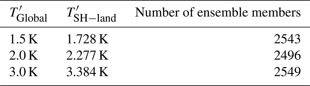
Three HAPPI (Half a degree Additional warming, Prognosis and Projected Impacts; see https://www.happimip.org/, last access: 4 July 2023) ensembles were used, representing climate states of 1.5, 2.0, and 3.0 K above pre-industrial global mean surface temperatures. There were approximately 2500 members for each ensemble, each 20 months long, of which we selected the last 12 months. In total, this provided approximately 7500 years of daily precipitation data for each location.

The $T_{\mathrm{Global}}^{\prime }$ values were converted to $T_{\mathrm{SH}-\mathrm{land}}^{\prime }$ using the MAGICC simulations (see Sect. 2.3). The mean of all $T_{\mathrm{Global}}^{\prime }$ entries was found across all scenarios (RCP2.6, RCP4.5, RCP6.0, RCP8.5, SSP119, SSP126, SSP245, SSP370, SSP434, SSP460, SSP585) and for each year from 1765 to 2150. The mean of all $T_{\mathrm{SH}-\mathrm{land}}^{\prime }$ entries was also found across all scenarios and for each year. The 1.5, 2.0, and 3.0 K $T_{\mathrm{Global}}^{\prime }$ values were interpolated to $T_{\mathrm{SH}-\mathrm{land}}^{\prime }$ values; see Table 5. We then use these $T_{\mathrm{SH}-\mathrm{land}}^{\prime }$ values in Sect. 5, when using weather@home.

Table 5 The annual mean global mean temperature anomalies associated with each HAPPI simulation, their Southern Hemisphere land temperature anomaly equivalents, and the number of members in each HAPPI ensemble.

3 Model description

Both the hourly and daily SPG use the same neural network and were assessed in a similar manner. The key differences between SPGs were the number of inputs to the neural network. Using a neural network allows for a simpler implementation, as seasonality and autocorrelation can be learnt without the need to explicitly account for them. In Sect. 3.6 we compare the neural network to a linear model.

3.1 Input features

For every hourly or daily observation in the data sets, several features were calculated to serve as predictors for the neural network. These features were selected, in part, through a process of trial and error to identify a parsimonious set of features that would provide robust predictability of the precipitation in the next time interval. Results from simpler network architectures informed our choice of the final set of predictors selected. The time span selected for specific features was based, in part, on the level of autocorrelation calculated from the precipitation time series; for example, it was found that there was little autocorrelation beyond 8 d (see Figs. 5 and 6). It is very likely that the set of features finally selected is not the optimal set of features, suggesting scope for future work to explore a far wider range of possible features. The features selected were combined with the observed precipitation for the period, effectively giving (X,y) training pairs, where X was a vector of features and y the observed precipitation amount for the period.

3.1.1 Daily features

The following 10 features were calculated for every day of daily observations in each station data set:

• average precipitation in the prior 1, 2, 4, and 8 d;

• average proportion of days with precipitation above a threshold (1 mm d⁻¹) in the previous 1, 2, 4, and 8 d;

• an annual cycle of variable phase, expressed as sine and cosine terms.

3.1.2 Hourly features

The following 16 features were calculated for every hour of hourly observations in each station data set:

• average precipitation in the prior 1, 3, 8, 24, 48, and 144 h;

• average proportion of hours with rain above a threshold (0.1 mm h⁻¹) over 1, 3, 8, 24, 48, and 144 h;

• an annual cycle and diurnal cycle, each expressed as a pair of sine and cosine terms.

3.1.3 Preprocessing features

The features were normalized by subtracting their mean and scaling by their standard deviation before they were fed as input to the neural network. If any of the prior days or hours were missing, this data point was removed from the training data set.

While the precipitation data, y, were scaled by the standard deviation, the mean was not subtracted as we wanted to ensure the precipitation remained positive. This scaling was reversed when producing a synthetic precipitation value (see Sect. 3.5).

3.2 Neural-network structure

Artificial neural networks (Kröse and van der Smagt, 1996) typically comprise may thousands of neurons, each of which calculates a weighted sum of all their inputs which is then transformed using an activation function. The neurons are arranged into layers: an input layer (with the number of neurons equal to the number of inputs), a number of intermediate – known as “hidden” – layers, and a final output layer (with the number of neurons equal to the number of desired outputs).

The neural networks underlying the SPGs took the features (described in Sect. 3.1) as inputs. The outputs of the network were used to specify parameters of precipitation distribution functions (described in Sect. 3.3). Several architectures of increasing complexity were developed and tested until a somewhat arbitrarily defined performance target was achieved. A full exploration of all possible architectural choices and their associated parameter spaces was not performed; there may well be superior architectures to that presented here. The results presented here indicate one possible approach, and we encourage the community to explore alternative and superior architectures.

The final architecture is described in Fig. 1.

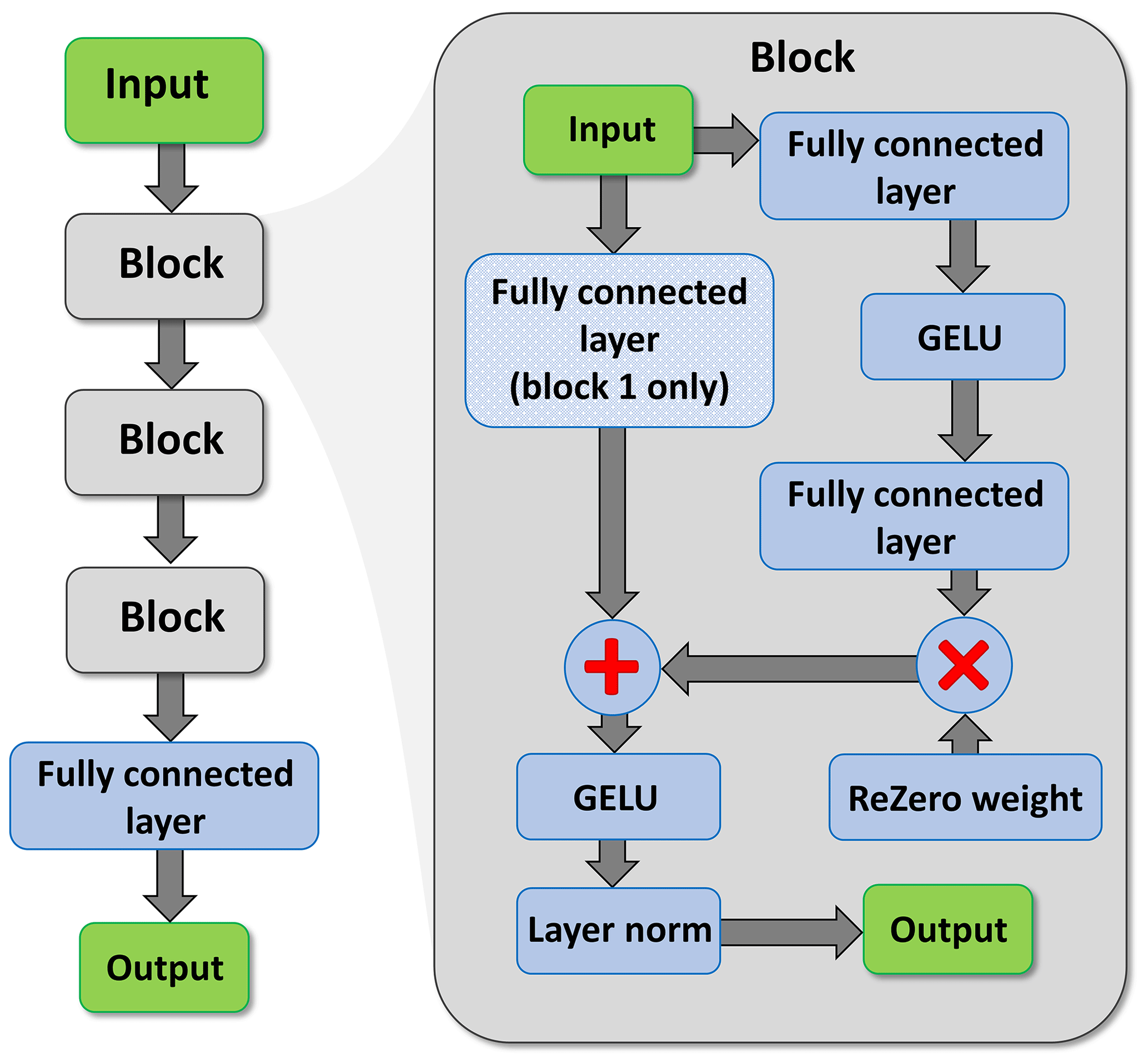
Figure 1 The neural-network architecture used in the daily and hourly SPGs. The inset on the right shows the detail of each of the three primary blocks shown on the left. Note that only the first block includes the fully connected layer on the identity path (downward arrow to the left of the block).

This architecture is based on that used in the construction of transformers (Wolf et al., 2020) but excluding the self-attention components. The internal structure of the network comprises three repeating blocks followed by a fully connected layer. The three hidden layers (“blocks” in Fig. 1) are each 256 neurons wide. The input received by each block immediately bifurcates along two different paths. The first, hereafter the identity path, passes the input directly to a ResNet (see below), while the second passes the data to a sandwich of a fully connected layer, a GELU activation function (Hendrycks and Gimpel, 2016), and then another fully connected layer. The output of this sandwich is multiplied by a very small weight, close to zero, and similar to the ReZero technique introduced by Bachlechner et al. (2021). This multiplication ensures that after the initialization, the intermediate layers of the neural network essentially just replicate their input, reducing the signal-to-noise ratio and aiding convergence. The output from the multiplication is combined with the identity path via a ResNet (shown with the + sign in Fig. 1). ResNets, known as residual neural networks, are typically arranged in blocks, where the input to a block is added back to the output of a block, giving an alternative path (the identity path) for gradients to flow and forcing the neural-network block to learn a residual on top of the input. Because they are easier to optimize and allow the training of deeper neural networks, ResNets are widely used within deep learning. The output from the ResNet feeds another GELU activation, and then finally layer normalization is performed. Layer normalization is a technique used to normalize the activations of intermediate layers (Ba et al., 2016) which helps stabilize the learning process and performs some regulation.

As the dimensionality of the input was not 256 (it was between 10 and 17; see Sects. 3.1 and 5), an extra fully connected layer was inserted on the identity path of the network to increase the dimensionality to 256. This ensures dimensional compatibility at the concatenation stage (+ sign in Fig. 1) in the first block. The neural network outputs a collection of real numbers; in Sect. 3.3 we discuss how these numbers are used to model precipitation. The neural networks underlying the SPGs were implemented using the machine-learning libraries JAX (Bradbury et al., 2018) and Flax (Heek et al., 2020). Each neural network comprises approximately 200 000 parameters, although the actual number of parameters differs slightly across SPG simulations, depending on the number of input features and the number of output values.

3.3 Neural-network outputs: precipitation distribution

For each period (either daily or hourly), the precipitation is simulated in two stages. The first stage selects whether precipitation occurs. Then, in the second stage, if precipitation did occur, the depth of precipitation is determined. The outputs from the neural network are used as parameters for both stages.

The first two network outputs (p_d and p_w) are used as parameters to model the probability of precipitation occurrence. Softmax, also known as the normalized exponential function, was applied to these first two parameters to ensure they represented probabilities (and always summed to 1, thus $p_{\mathrm{w}}=\mathrm{1}-p_{\mathrm{d}}$). The first parameter, p_d, represents the probability that the period was dry, and the second parameter, p_w, represented the probability of a wet period.

If precipitation occurred, another distribution was used to model the depth of the precipitation. Katz (1977) previously employed a gamma distribution to model precipitation. We found that a mixture of two gamma distributions and two generalized Pareto distributions provided a superior fit as this combination avoided overfitting while still appropriately capturing the likelihood of extreme precipitation. This is not the case when using a single gamma distribution which significantly underestimates extreme precipitation. Other mixtures of distributions, including Weibell distributions, were tested. Mixtures incorporating Weibell distributions tended to generate excessively large extreme precipitation (unbounded) values and so were discarded; minimizing the loss was not the only factor used to select the optimal mix of distributions.

Some parameters learned by the model such as the scale and shape parameter of the gamma distributions are required to be positive. To ensure such constraints, they were passed through elu(x)+1, where elu(x) is the exponential linear unit function (Clevert et al., 2015). For the generalized Pareto distribution, the location parameter was set to zero, and both the shape and scale were forced to be positive. While the shape can conceivably be negative for a generalized Pareto distribution, allowing it to be negative led to training instabilities. This resulted in two parameters being used for each of the four distributions, with a further four parameters being used to weight the distributions within the mixture, for a total of 12 parameters used to model the amount of precipitation. Again, we applied softmax to the weightings of the mixture model to ensure they summed to one.

Equation (1) shows the log probability density function used within the loss function (Sect. 3.4). The probability of a dry period (either day or hour) is given by p_d, and p_w is the probability of a wet period, while r is the rain period threshold, i.e. the threshold under which the period is considered dry. The rain period threshold was set to 1.0 mm d⁻¹ for the daily data set and 0.1 mm h⁻¹ for the hourly data set. A threshold of 0.1 mm d⁻¹ for the daily data was found to lead to poor performance in the precipitation extremes. The variable y is the precipitation from the training data set, P_i is the probability density function of distribution i in the mixture model, and w_i is the weighting of the corresponding component in the mixture model. In this case, n is set to four, as there are four distributions in the mixture model. For each distribution in the mixture, $y-r+\mathit{ϵ}$ is passed to the corresponding probability density function. Each distribution is designed to model positive values. We add r back to the precipitation depth when sampling (see Sect. 3.5), and we set ϵ to 10⁻⁸ for numerical stability.

$$\begin{array}{}\text{(1)}& \log \mathit{\_}\mathrm{pdf}\left(y\right)=\left\{\begin{array}{ll}\ln \left(p_{\mathrm{d}}\right)& \text{if }y<r\\ \ln \left(p_{\mathrm{w}}\right)+\ln \left({\sum }_{i=\mathrm{1}}^n\right(w_i{P}_i(y-r+\mathit{ϵ}))& \text{if }y\mathit{>=}r\end{array}\right.\end{array}$$

3.4 Training

A single station's observed precipitation data were used in every training run. In training the daily SPG, the last 1000 entries (not quite 3 years) were kept aside for validation. In training the hourly SPG, the last 10 000 entries (slightly more than a year) were used for validation. A one-step-ahead prediction over the last 1000 or 10 000 observations was used to calculate the validation loss. The remainder of the data were used for training. The batch size was set to 256, and therefore 256 samples from the training data set were evaluated every training step. The mean negative log-likelihood (the negative mean of Eq. 1 across a batch) was used as the training loss function, and the model was trained for up to 40 epochs. Although minimizing the negative log-likelihood is equivalent to maximizing the likelihood, using the log-likelihood results avoids numerical underflow when dealing with small probabilities as it requires a summation as opposed to a product. The training process can be thought of as the neural network trying to produce the parameters for Eq. (1) that maximize the probability of observing the precipitation in the training data sets given the corresponding features (Sect. 3.1).

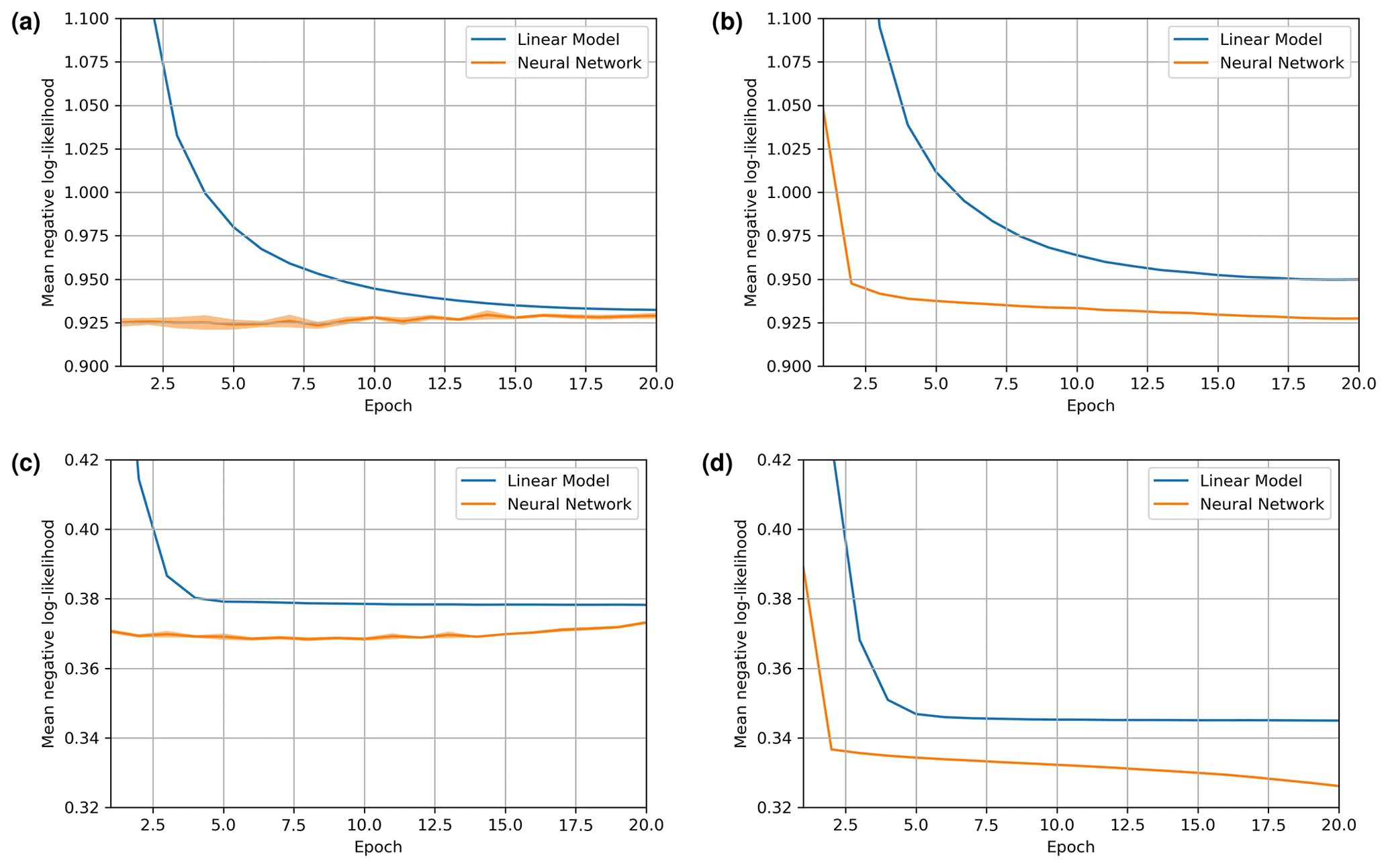
Figure 2 (a) Mean validation loss for the daily SPG, (b) mean training loss for the daily SPG, (c) mean validation loss for the hourly SPG, and (d) mean training loss for the hourly SPG. All SPGs were trained for Auckland. The mean of five training runs are shown with 95 % confidence intervals displayed as shading; the confidence intervals are not always visible as the uncertainties are very small.

The neural network was optimized using Lookahead (Zhang et al., 2019), with AdamW (Loshchilov and Hutter, 2017) as the inner optimizers, a weight decay of 0.01, b1 of 0.9, and b2 of 0.999. Lookahead was configured with a slow weight step of 0.5 and a synchronization period of five steps. A cosine learning rate scheduler was used, with a maximum learning rate of 10⁻³ and a minimum learning rate of 10⁻⁷, with a warm-up from 10⁻⁶ to 10⁻³ for the first 300 training steps. The maximum number of decay training steps, after which the learning rate would stay at the minimum, was set to 5000 for training the daily SPG and 50 000 for training the hourly SPG. We used the implementation from the Optax library (Hessel et al., 2020) to configure our optimizer.

3.5 Generating precipitation time series

To validate the SPGs through comparisons with the observed station data, precipitation series were generated by the SPGs over the same time range as the historical data set but without any gaps. To initiate the simulation, the first 8 d of precipitation for the daily SPG or the first 144 h for the hourly SPG were extracted from the observations. These were used to calculate the inputs for the neural network (as per Sect. 3.1), which then iteratively generates the next day or hour of precipitation. This next data point is then appended to the precipitation series. The extended time series is then used to calculate the input features for the next hour or day, in a sliding window manner.

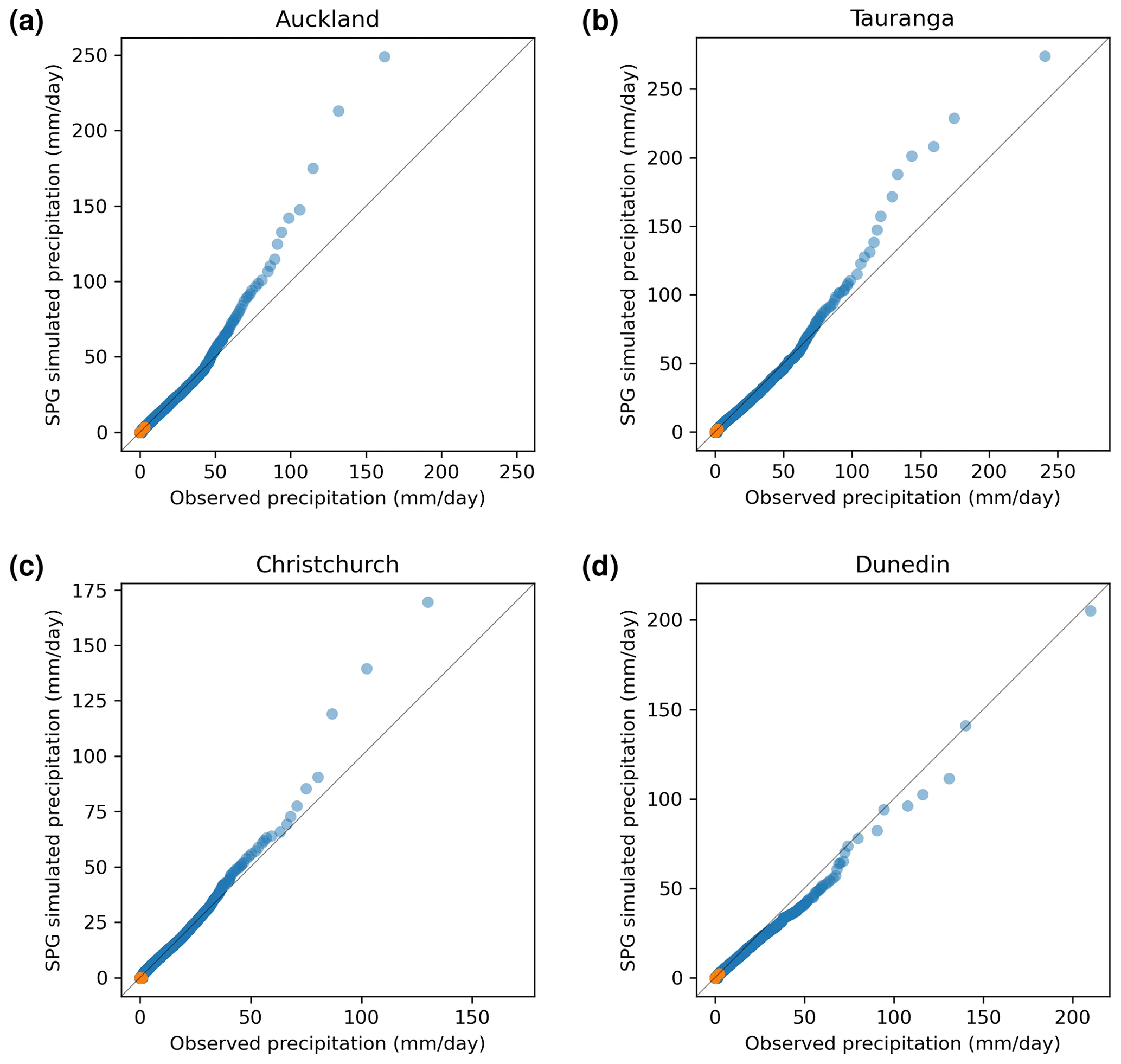
Figure 3 Quantile–quantile plots of simulated precipitation produced by the daily SPG against observed precipitation. Orange points indicate quartiles.

Recall that the neural network generates 14 parameters which are then used to generate the precipitation distribution (Eq. 2). To generate a precipitation time series, we sample from this distribution using two random uniform numbers, u₁ and u₂. u₁ is used to sample from the dry-day part of the distribution. If u₁ is smaller than p_d (the probability of a dry day – the first parameter from the neural network), the precipitation is set to zero. If u₁≥p_d, the precipitation depth is sampled from the mixture using u₂; i.e. we sample from the mixture of size n (in this case four) by summing the quantile function (also known as the percentage point function), Q_i, at u₂ of each mixture and multiplying it by its corresponding weight (w_i). The mixture model distributions were constructed as described in Sect. 3.3. Finally, we add r back to the precipitation as we had previously subtracted it, as described in Sect. 3.3. Therefore, the daily SPG does not produce non-zero precipitation below 1 mm d⁻¹, and the hourly SPG does not produce non-zero precipitation below 0.1 mm h⁻¹.

$$\begin{array}{}\text{(2)}& y_{\mathrm{pred}}=\left\{\begin{array}{ll}\mathrm{0}& \text{if }{u}_{\mathrm{1}}<p_{\mathrm{d}}\\ r+{\sum }_{i=\mathrm{1}}^n\left(w_i{Q}_i\right(u_{\mathrm{2}})& \text{if }{u}_{\mathrm{1}}\ge p_{\mathrm{d}}\end{array}\right.\end{array}$$

Very rarely, the SPG produces invalid precipitation values or precipitation values much too high. We used expert judgement to prescribe upper bounds on the maximum daily and hourly precipitation accumulations for each location (see Table 6). If the accumulated precipitation exceeded the bound for the given location or if the precipitation was invalid, then the precipitation was sampled from the mixture model again.

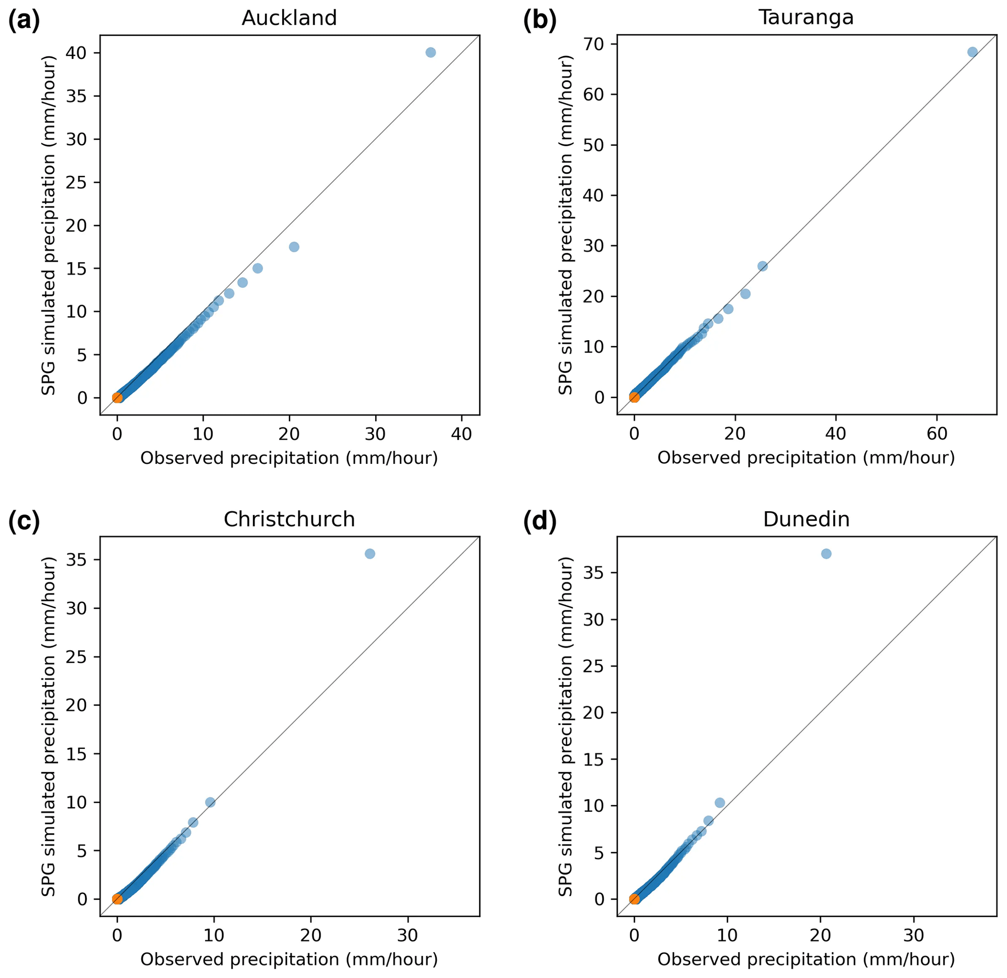
Figure 4 Quantile–quantile plots of simulated precipitation produced by the hourly SPG against observed precipitation. Orange points indicate quartiles; these are generally too close to zero to distinguish.

Table 6 Imposed maximum daily and hourly precipitation for the given locations, for the daily SPG and hourly SPG, respectively.

3.6 Neural network versus linear model

A common question that arises when creating a neural-network-based SWG is whether using a neural network actually improves the performance of the model. To investigate this, the neural network within each of the SPGs was replaced with a single linear layer, including a bias, with everything else left the same. Despite replacing the neural network with a single linear layer akin to multiple linear regression, the problem is still formulated as a non-linear optimization problem due to the complex distributions used within the mixture model. Both the linear and neural-network-based SPG were trained on the hourly and daily Auckland data sets, with five different random seeds. The results were then averaged.

The mean validation loss and training loss for the daily and hourly SPGs using the linear model and the neural-network-based model are shown in Fig. 2. Given the relatively large volume of data available for training, the mean validation loss approached the minimum loss within the first epoch. For the daily SPG, the neural network achieved a minimum average validation loss of 0.926, while the linear model achieved a minimum average validation loss of 0.932, showing the superior performance of the neural-network-based SPG. For the hourly SPG, the neural network achieved a loss of 0.369 while the linear model achieved a loss of 0.378, again showing the superior performance of the neural-network-based SPG. The neural network also converges much faster than the linear model. The mean negative log-likelihood minimizes within the first few epochs (generally before or at epoch 6 for the daily SPG and epoch 10 for the hourly SPG – depending on which of the five ensemble members are considered). Thereafter, the neural network begins to slightly overfit, indicated by the validation loss starting to increase while the training loss continues to decrease. It is therefore important to employ early stopping when training the neural network. Hereafter, we report only results generated by the neural-network-based SPGs.

4 Stationary SPG quality assessment

4.1 Quantile–quantile comparisons

Quantile–quantile (QQ) plots of SPG-simulated precipitation against station-observed precipitation provide a measure of any biases in the magnitude of the precipitation simulated by the SPG. Ideally, points on the QQ plot should lie on the y=x line but due to the stochastic nature of the SPGs; some deviation from this line is to be expected. QQ plots for the four sites are shown in Fig. 3 for the daily resolution SPG and in Fig. 4 for the hourly resolution SPG. For most days, there is no precipitation – for the cities studied, on average, it is dry (less than 1.0 mm d⁻¹) 68 % of the time. For hourly precipitation, it is dry (less than 0.1 mm h⁻¹) 96.9 % of the time. As a result, the 25th percentile and 50th percentile (equivalent to the median) are usually zero as shown by the orange dots in Figs. 3 and 4.

The QQ plots in Figs. 3 and 4 show that the SPGs approximate very well the original distributions of precipitation intensity. The daily SPG overestimates the extremely high precipitation (>50 mm d⁻¹) values over Auckland, Tauranga, and Christchurch by 10±14 % but shows little, if any, bias for Dunedin. For the hourly SPG, at all four sites, there is no significant bias against the observations.

For both the daily and hourly SPG, it is clear that precipitation depths outside the range of the training data can be simulated.

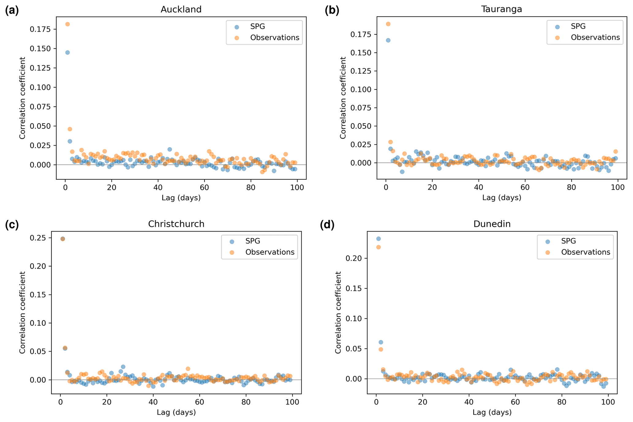
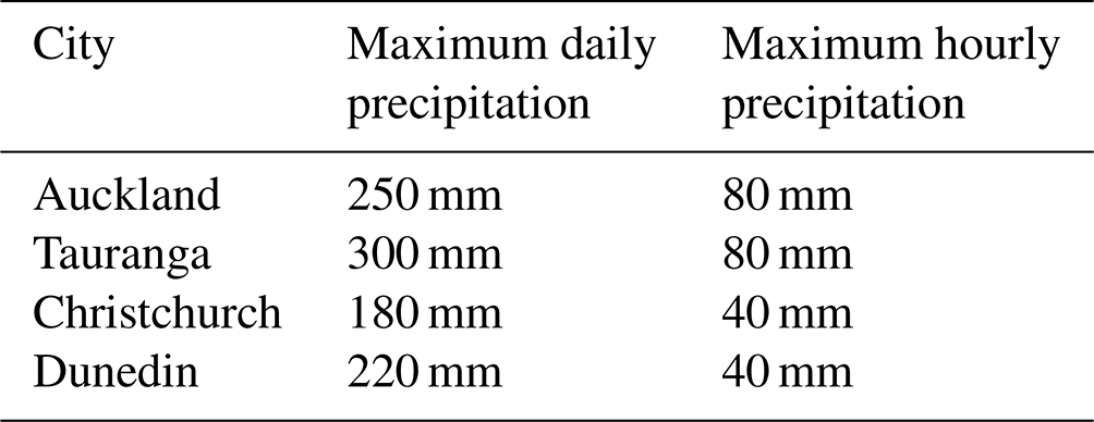
Figure 5 Autocorrelation plots for precipitation simulated by the daily SPG and for observed precipitation.

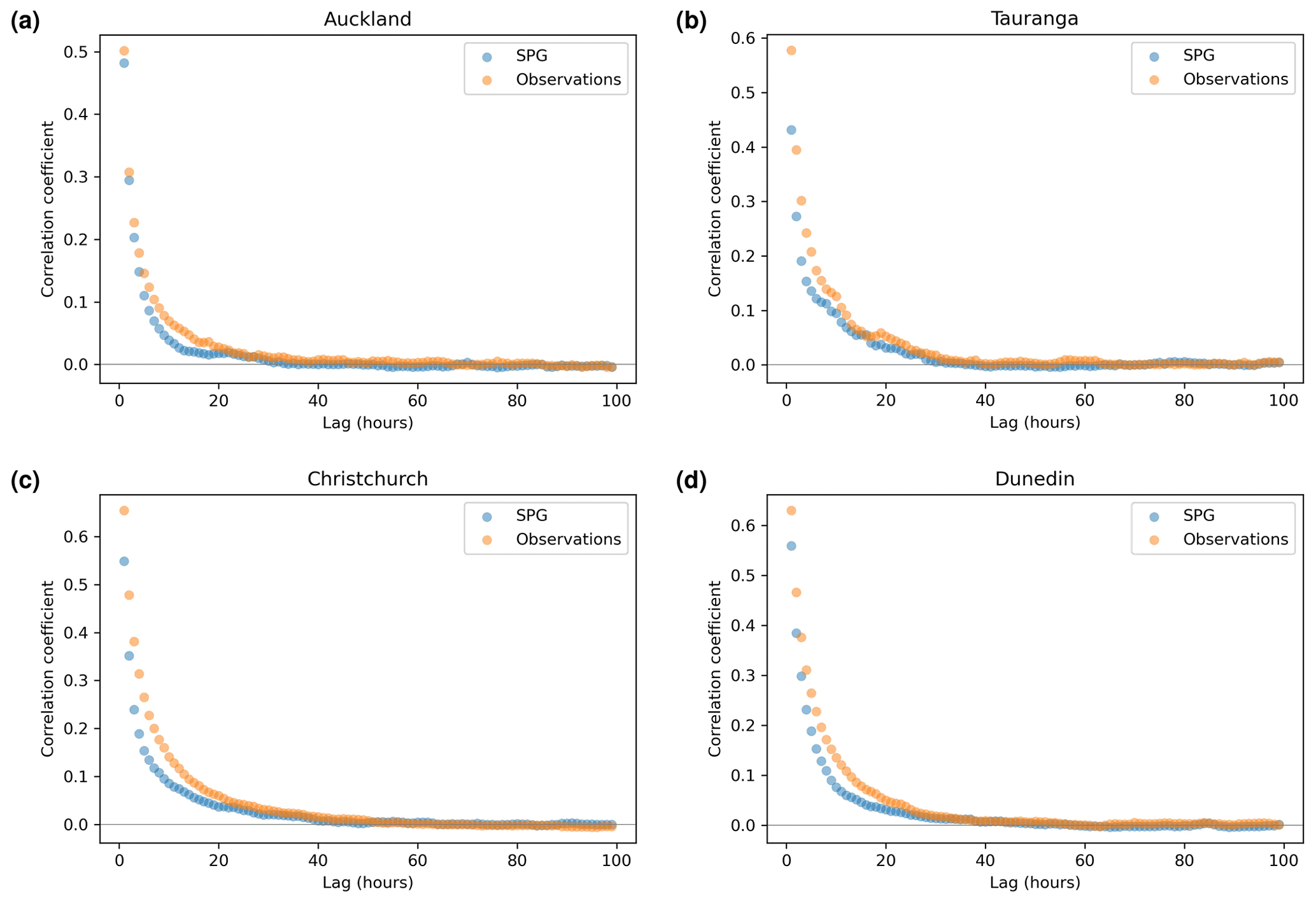
Figure 6 Autocorrelation plots for precipitation simulated by the hourly SPG and for the observed precipitation.

4.2 Autocorrelation

While the QQ plots are useful for assessing the extent to which the SPGs can simulate the correct distribution of precipitation intensity, they are agnostic to the sequence of the precipitation and provide no assessment as to whether the cadence of precipitation is simulated correctly. To that end, we first consider the extent to which the SPGs can simulate the autocorrelation observed in the precipitation time series. Correlation coefficients for the daily SPG for all fours sites for a range of lags (in days) are shown in Fig. 5. The equivalent coefficients for the hourly SPG are shown in Fig. 6.

In general, the daily SPG does an excellent job in replicating the observed autocorrelation and slightly underestimates the autocorrelation in the hourly SPG. At Auckland, the daily precipitation observations show low but non-zero levels of autocorrelation all the way out to about 70–80 d lag (Fig. 5a). This is likely caused by the strong seasonality in precipitation seen in Auckland (Sect. 5.4). The daily SPG appears to simulate well that structure in the autocorrelation.

4.3 Dry-spell duration and cadence

Another precipitation cadence attribute which is important for the SPGs to simulate correctly is the dry-spell length, i.e. the number of consecutive days where precipitation is less than 1.0 mm d⁻¹. This is essential if the SPG is to be used to simulate drought conditions for any location. To that end, Fig. 7 shows QQ plots of dry-spell length for all four locations. The daily SPG shows an excellent ability to simulate correctly the frequency of dry-spell lengths at all four locations. The deviations from 1:1 correspondence at the longer dry-spell lengths (the rightmost few data points of the 10 000 data points describing the quantiles) most likely result from the stochastic nature of the SPGs. This suggests that this SPG could form the basis for drought-based studies if more variables describing key drought parameters, such as temperature and solar radiation, were added.

To produce the dry-spell QQ plots for the hourly SPG shown in Fig. 8, both the station data and the SPG-simulated data were first resampled to daily frequency prior to calculating the dry-spell lengths. The hourly SPG also shows strong skill in simulating dry-spell lengths with perhaps a small underestimation for Tauranga and overestimations at the very longest dry-spell lengths for Auckland, Christchurch, and Dunedin.

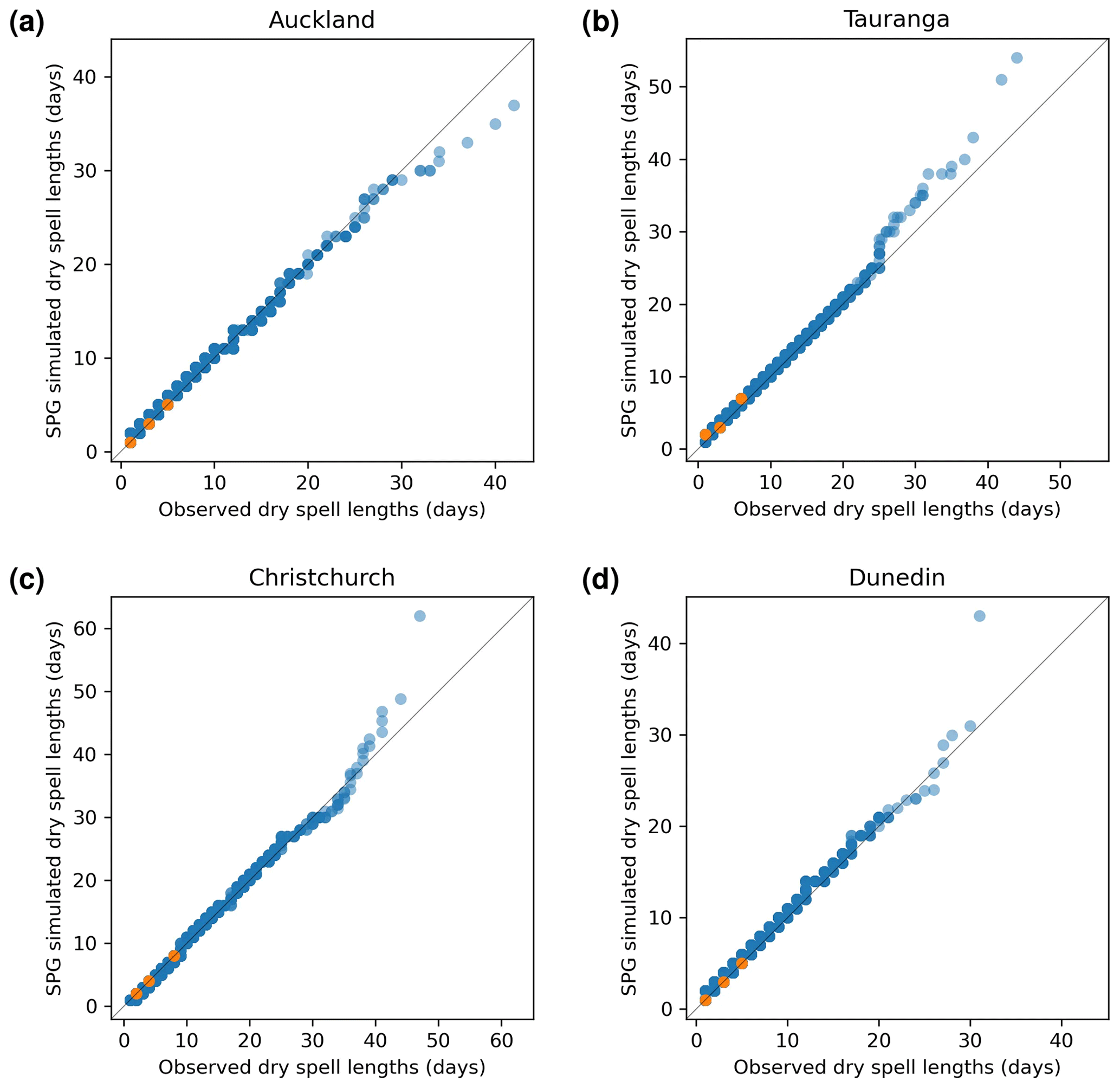
Figure 7 Quantile–quantile plots for simulated dry-spell lengths produced by the daily SPG against observed dry-spell lengths. Orange points indicate quartiles.

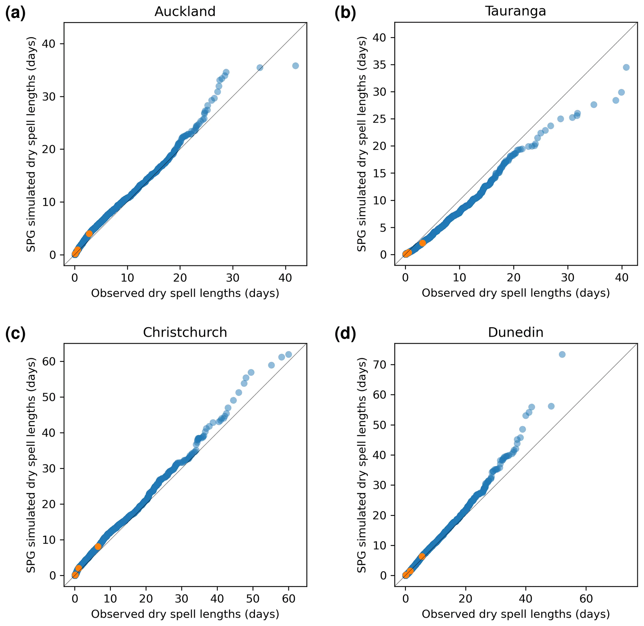
Figure 8 Quantile–quantile plots for simulated dry-spell lengths produced by the hourly SPG against observed dry-spell lengths. Orange points indicate quartiles.

4.4 Seasonality

To assess whether the SPGs simulate the seasonality of the precipitation correctly, dry-day seasonality was calculated as the proportion of days in a given week of the year that had less than 1.0 mm d⁻¹ of precipitation. The dry-hour seasonality was calculated similarly but with a threshold of 0.1 mm h⁻¹. We focused on dry-day seasonality, as there was little seasonality in the wet-day precipitation depths.

Auckland displays the strongest seasonality in dry-day proportions, and the daily SPG simulates this seasonality extremely well (see Fig. 9a). The dry-hour proportions from the observations for Auckland (Fig. 10a) showed a weaker, more noisy signal compared to the daily observations. This was likely caused by the far shorter hourly observation period (around half the number of years). The hourly SPG somewhat underestimates the seasonality in the proportion of dry hours for Auckland (Fig. 10a).

Tauranga also shows a strong daily seasonal cycle in the proportion of dry days, which was also excellently simulated by the daily SPG (Fig. 9b). The hourly SPG captures, to some extent, the weak seasonal cycle in the proportion of dry hours in Tauranga.

While neither Christchurch (Fig. 9c) nor Dunedin (Fig. 9d) shows strong seasonality, the daily SPG simulates their weak seasonality well.

Christchurch appears to have a more clear seasonality in the proportion of dry hours (Fig. 10c) that was simulated well by the hourly SPG, albeit with a small offset. The hourly SPG simulates well the lack of seasonality in Dunedin's proportion of dry hours, although also with a slight offset (Fig. 10d).

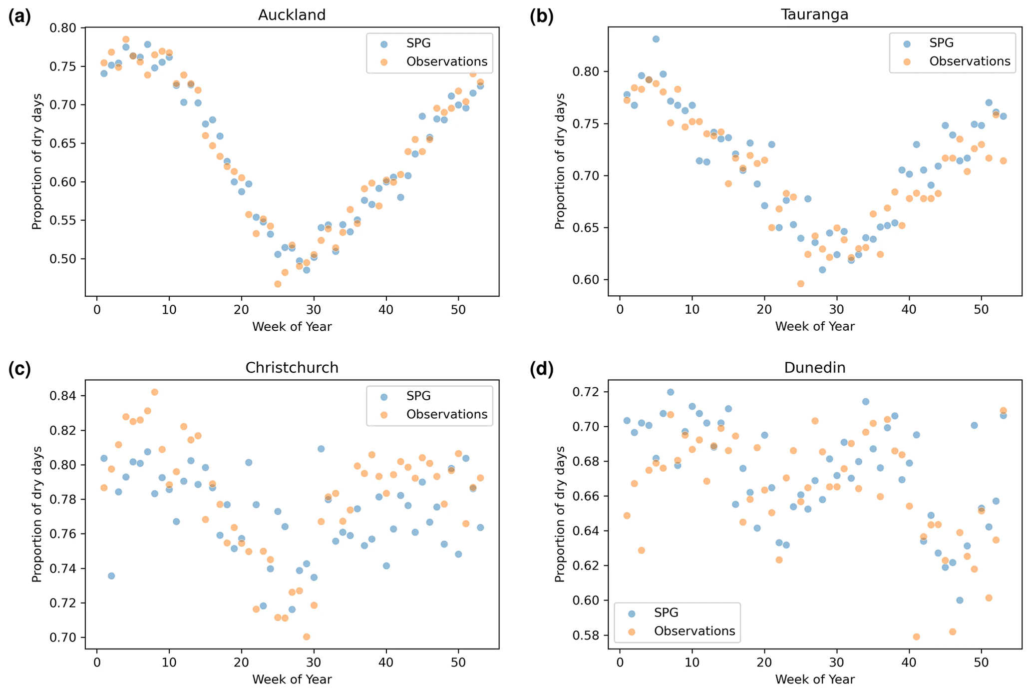
Figure 9 Dry-day proportion (proportion of days in a given calendar week of the year with precipitation less than 1 mm d⁻¹) against the week number of the year.

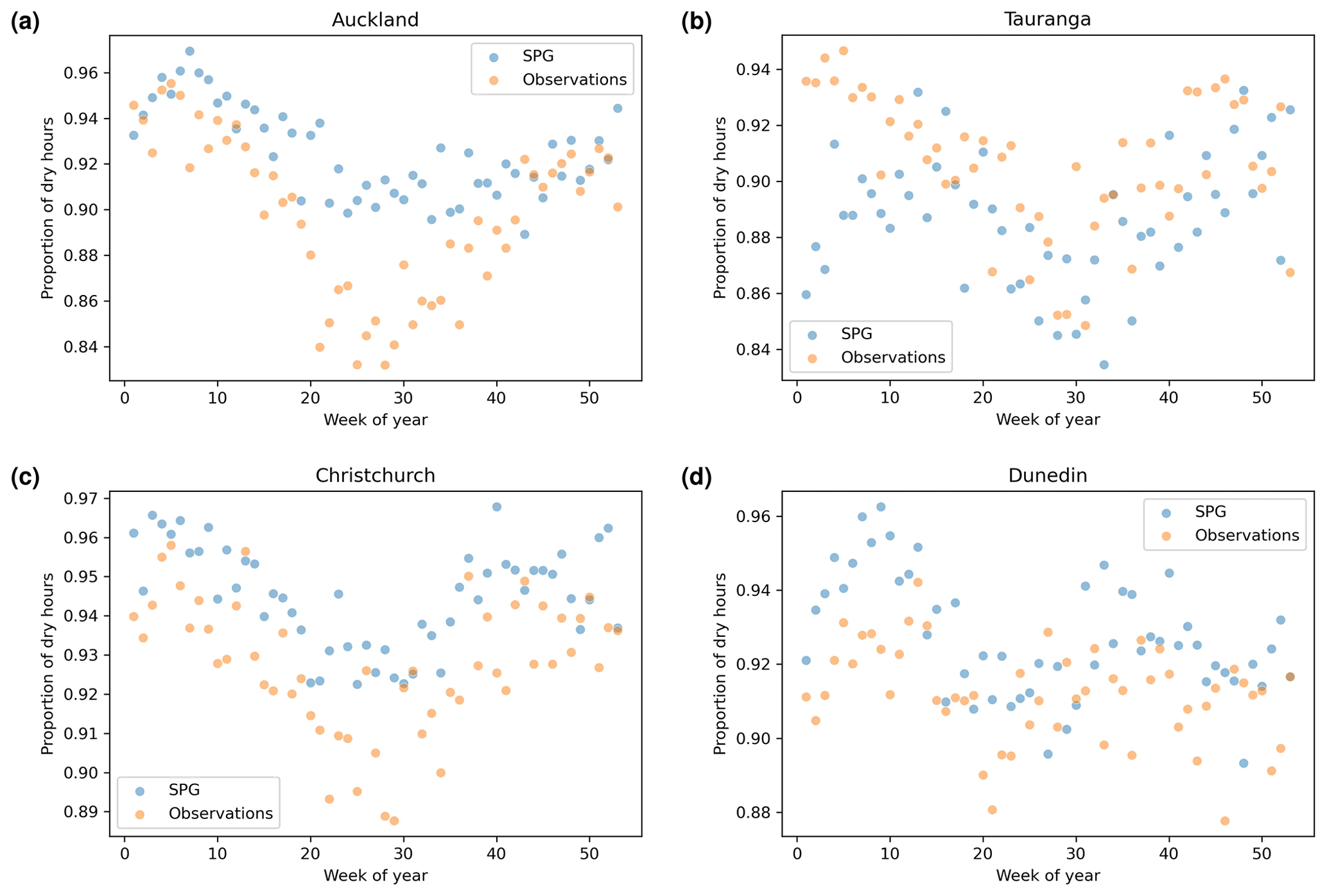
Figure 10 Dry-hour proportion (proportion of hours in a given calendar week of the year with precipitation less than 0.1 mm h⁻¹) against the week number of the year.

Table 7 One-day precipitation extremes for 10- and 100-year return periods, calculated from the daily observations and a large ensemble from the daily SPG. The 90 % confidence bounds for the observation are shown in square brackets.

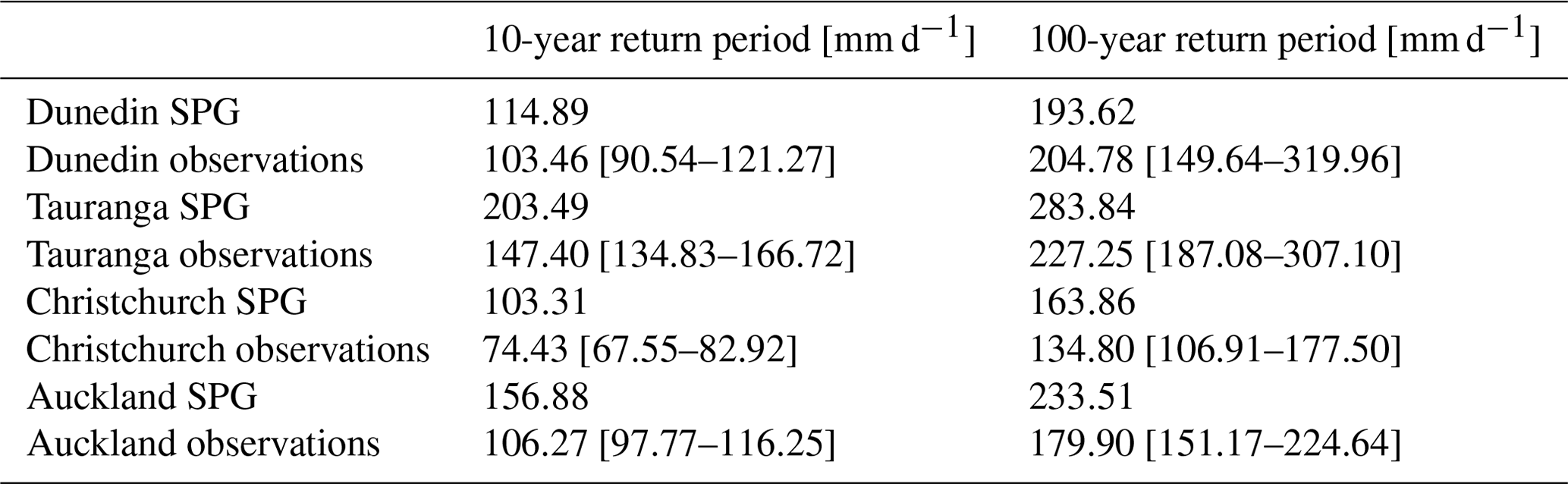
Table 8 One-hour precipitation extremes for 10- and 100-year return periods, calculated from the hourly observations and an hourly ensemble from the daily SPG. The 90 % confidence bounds for the observation are shown in square brackets.

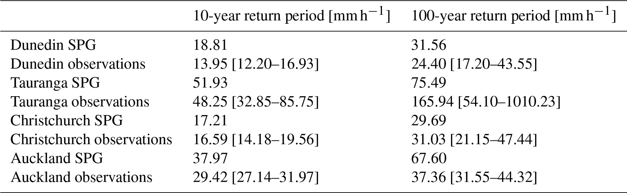
Table 9 Precipitation statistics calculated from the daily observations and a large ensemble from the daily SPG. The 90 % confidence intervals are given for annual precipitation and wet proportion.

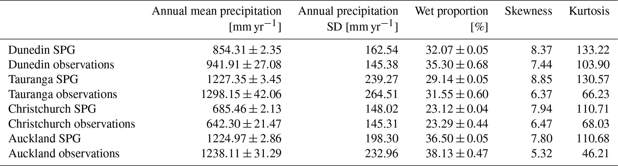
Table 10 Precipitation statistics calculated from the hourly observations and a large ensemble from the hourly SPG. The 90 % confidence intervals are given for annual precipitation and wet proportion.

4.5 Statistical summary

We generated a large ensemble of daily and hourly SPG simulations, totalling over 13 000 years of precipitation data, for each location. To analyse the extremes for the SPG simulations, and given the large volume of data, we did not need to fit extreme value distributions but rather simply took annual block maximum and then calculated precipitation depths (mm d⁻¹ and mm h⁻¹) for 10-year and 100-year return periods directly from quantiles of the block maxima (see Tables 7 and 8). For the observations, however, with a single time series, it was necessary to fit generalized extreme value (GEV) distributions to the 1-year block maxima (Coles, 2001). The 90 % confidence intervals were calculated using a parametric bootstrap. Overall, the daily SPG performs adequately in simulating the extremes. However, there is some overestimation of the extremes at Auckland and Tauranga. The hourly SPG accurately reproduces the extremes at all locations, except for Auckland, for which there is some overestimation. The middle and upper-bound estimates for the observations at Tauranga are very likely too high as a result of the exceptionally short hourly precipitation record available at this location (only 24 years of data). All the other locations have a sufficient volume of data to produce reasonable estimates.

Tables 9 and 10 summarize various other statistics for the daily and hourly precipitation data, respectively. We used the same large SPG ensemble as above but apply the same methodology to both the observations and the SPG simulations when calculating these statistics. The wet proportion represents the percentage of the year when it is raining on any given hour or day. We used a threshold of 1.0 mm d⁻¹ for the daily precipitation and 0.1 mm h⁻¹ for the hourly precipitation. Both the wet proportion and the annual precipitation were first calculated on an annual basis, the means derived, and the 90 % confidence intervals calculated. The daily SPG accurately captures the annual precipitation and wet-day proportion. The standard deviation of annual mean precipitation was also calculated to understand whether the SPG produced sufficient year-to-year variability, as the SPG has no intrinsic input features to capture this variability. Table 9 suggests that the daily SPG largely captures this variability, with only small underestimation in Auckland and Tauranga. The hourly SPG, whose statistics are summarized in Table 10, underestimates the variability at all locations. This may be largely due to the SPG underestimating the annual mean precipitation at all locations, except Tauranga. The poor performance of the hourly SPG, compared to the daily SPG, on the annual precipitation is likely due to a poor estimate of the wet-day proportion. Improving how the hourly SPG estimates the wet-hour probability is a target for future development of our SPG.

5 Non-stationary extensions

The SPG described in Sect. 3 and whose results are presented in Sect. 4 is a stationary SPG, i.e. the statistics of the precipitation that it generates are time invariant. As such, the SPG is insensitive to climate change and will represent the mean precipitation climate over the period of data on which it was trained. The purpose of this section is to describe extensions to the SPG that make it non-stationary and therefore amenable to simulating climate-induced changes to the statistics of the precipitation.

Daily (and hourly) values of $T_{\mathrm{SH}-\mathrm{land}}^{\prime }$ were obtained by repeating the annual value for that year and were fed as an extra feature to both the daily and hourly SPGs to create daily and hourly non-stationary SPGs. This resulted in the daily, non-stationary SPG having 11 input features and the hourly, non-stationary SPG having 17 input features (see Sect. 3.1.1 and 3.1.2 for a discussion of the other features). Other than the addition of the new input futures based on $T_{\mathrm{SH}-\mathrm{land}}^{\prime }$, the model architecture and training were the same as for the stationary SPG.

A similar set of validation plots, as for the daily and hourly stationary SPG, were created for the non-stationary SPGs. Since there were no substantive differences between the stationary and non-stationary validation plots, they are not included here.

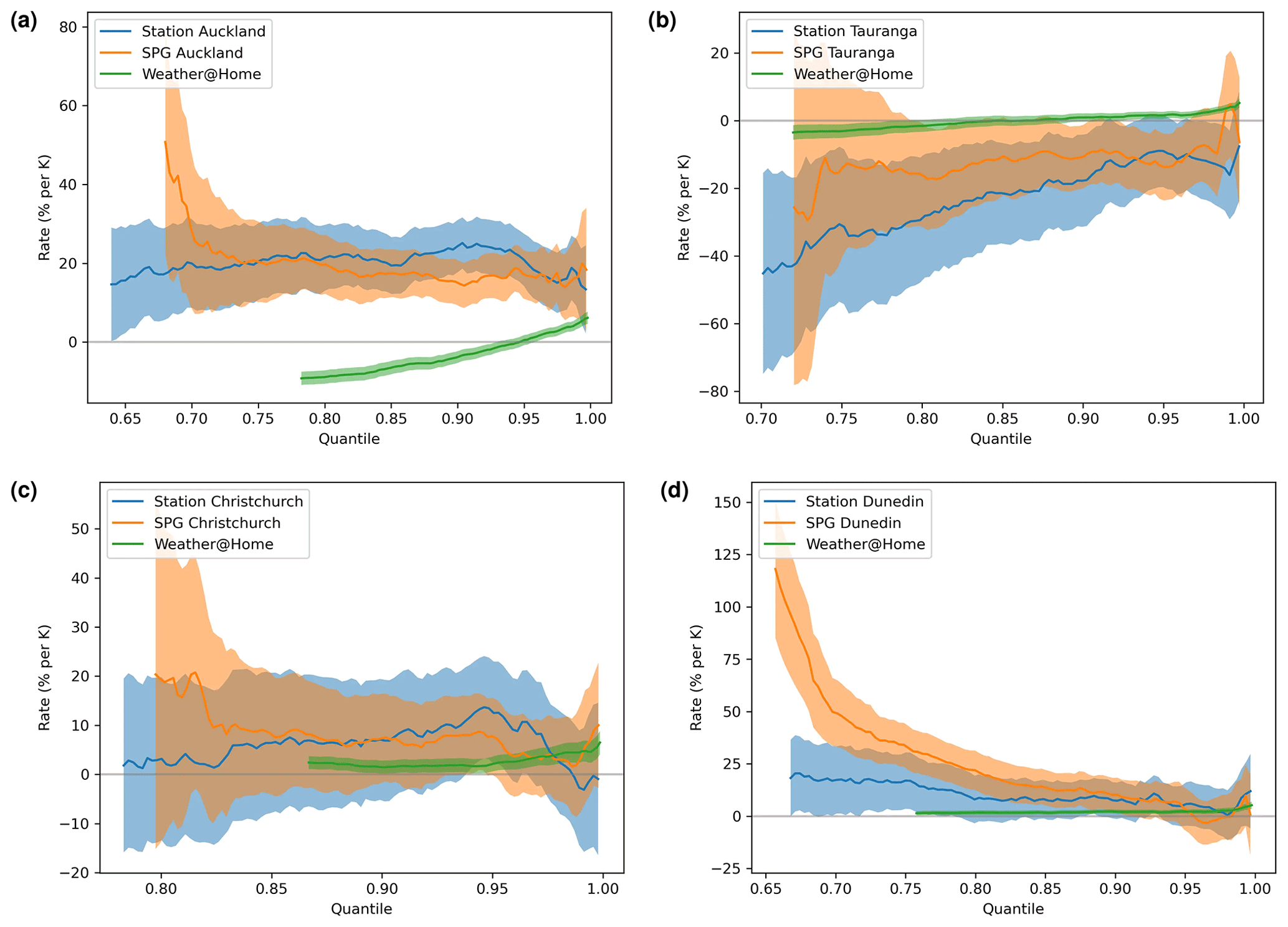
Figure 11 The percentage precipitation change per kelvin change in $T_{\mathrm{SH}-\mathrm{land}}^{\prime }$ for the daily SPG across all four sites over the same period as the historical observations (orange) together with comparable rates derived from the historical observational record (blue) and from weather@home simulations provided at daily resolution (green). Shading indicates 95 % confidence intervals (note the smaller uncertainties resulting from the large ensembles available from weather@home). All three data sets are truncated to precipitation above 1.2 mm d⁻¹. Because weather@home simulates many days with extremely low precipitation, i.e. below an observable detection limit, there are fewer percentiles exceeding 1.2 mm d⁻¹.

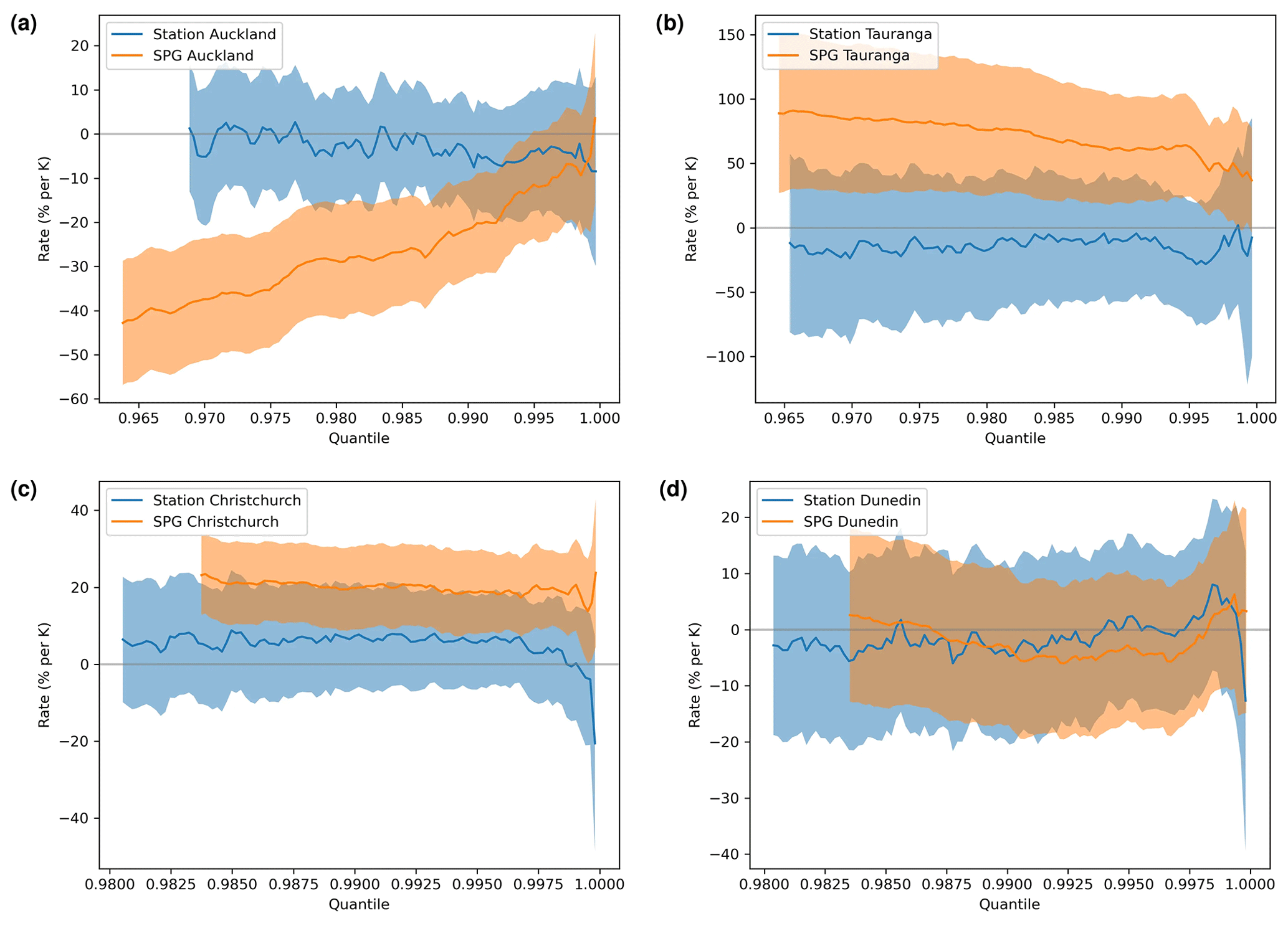
Figure 12 As for Fig. 11 but for the hourly SPG. Results for weather@home are not included as hourly precipitation data were not saved for the weather@home simulations.

5.1 Assessing the validity of the non-stationarity in precipitation

To quantify the non-stationarity in precipitation in (i) the SPG simulations, (ii) the weather@home simulations, and (iii) the observations, we calculated within each year of data 100 quantiles of precipitation. These were then analysed independently for the percentage change in precipitation per 1 K change in $T_{\mathrm{SH}-\mathrm{land}}^{\prime }$. This arose from expectations of the application of the Clausius–Clapeyron equation of a 7 % change in atmospheric water vapour loading for every 1 K change in temperature. We recognize that the same sensitivity cannot be expected for precipitation but that a similar functional dependence (but with different rates) may be expected. A comparison of rates extracted from SPG simulations with rates extracted from observations and/or RCM simulations comprises our assessment of the validity of the non-stationarity in precipitation simulated by the SPG. Where this method was applied to the weather@home RCM simulations containing many ensemble members, the annual mean ensemble mean was calculated for each calendar year. To each of these time series we fitted p(T)=p₀e^rT, where p(T) is the precipitation at a $T_{\mathrm{SH}-\mathrm{land}}^{\prime }$ value of T; p₀ is the expected precipitation when $T_{\mathrm{SH}-\mathrm{land}}^{\prime }$ is zero, i.e. in 1765; and r is the rate of change per kelvin. An example of the fit of this function to the 75th percentile of precipitation extracted from the weather@home simulations for Auckland is shown in Sect. 5.3 and Fig. 14.

5.2 Quality assessment

The rates described in Sect. 5.1 were calculated across all 100 quantiles for both the daily SPG (see Fig. 11) and the hourly SPG (Fig. 12). The uncertainties on the traces shown in these figures as well as Fig. 13 were calculated from uncertainties on the fit of the p(T)=p₀e^rT equation to the data within each of the 100 quantiles.

For the daily SPG these are compared with equivalent rates derived from the observations and from the weather@home simulations. Because the weather@home simulations provide output only at daily resolution, for the hourly SPG the derived rates are compared only with observationally determined rates in Fig. 12.

The precipitation sensitivities to $T_{\mathrm{SH}-\mathrm{land}}^{\prime }$ simulated by the daily SPG are generally not statistically distinguishable from those derived from the observational record (although the uncertainties on both are large). They are, however, often statistically significantly different from those derived from the weather@home simulations. There are also significant inter-site differences: consider Auckland and Tauranga, which are just 150 km apart. Auckland shows large positive precipitation sensitivities to changes in $T_{\mathrm{SH}-\mathrm{land}}^{\prime }$, while Tauranga shows large negative sensitivities. At both sites the sensitivities are quite different from those derived from the weather@home simulations.

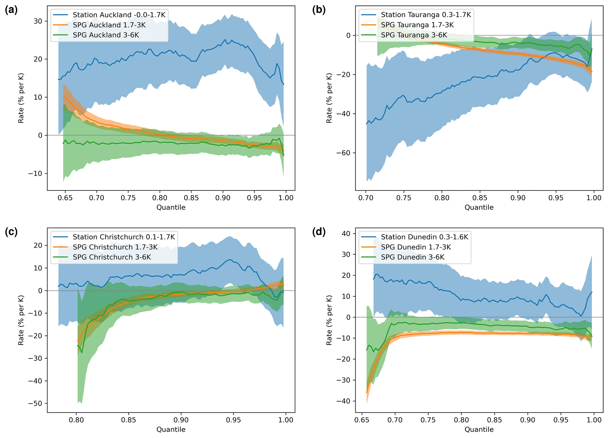
Figure 13 SPG-derived precipitation rates/sensitivities in percent per kelvin (% K⁻¹) for each quantile with daily change (per kelvin) versus quantiles; 95 % confidence intervals shown as filled areas. Only precipitation quantiles with more than 1.2 mm h⁻¹ were plotted. We focus on the projected changes of the difference range of $T_{\mathrm{SH}-\mathrm{land}}^{\prime }$. The minimum and maximum historical $T_{\mathrm{SH}-\mathrm{land}}^{\prime }$ values are also shown for each station. These plots demonstrate that the daily, non-stationary SPG does not perform as expected when predicting values into the future (1.7–6 K). Some temperature values for the station data were just below 0 K because there were years that were cooler than the reference year, due to temperature fluctuations.

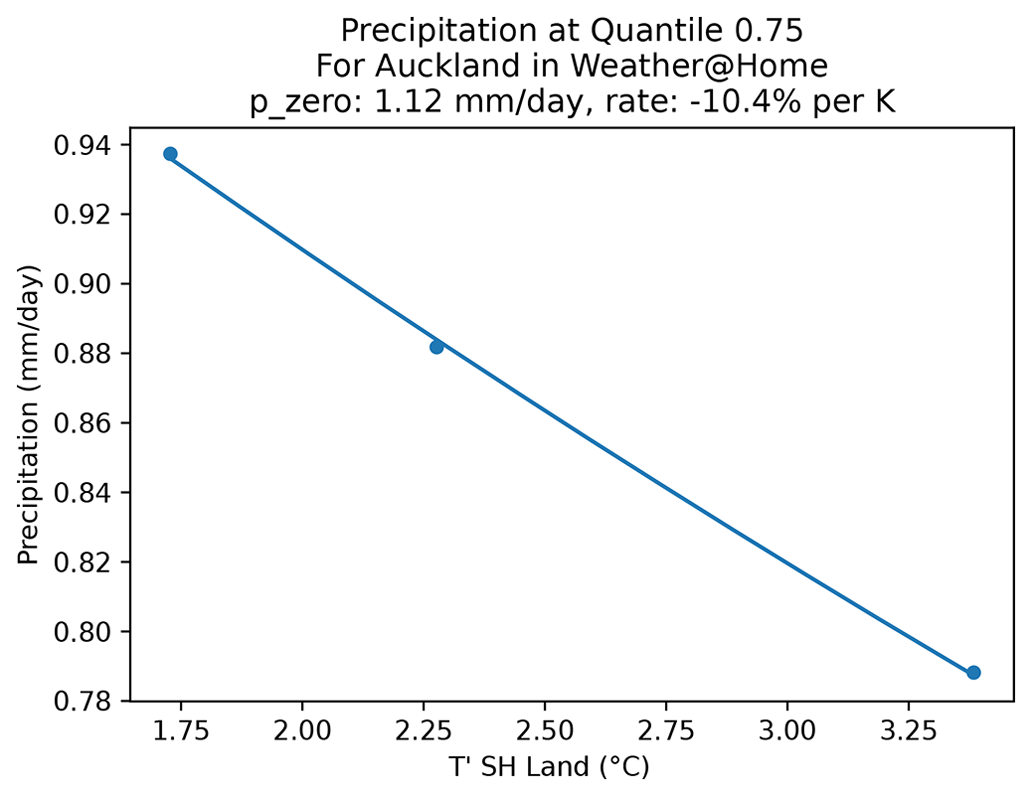
Figure 14 The ensemble mean, weather@home precipitation at the 75th percentile in Auckland, and the fit used to extract the sensitivity of precipitation to $T_{\mathrm{SH}-\mathrm{land}}^{\prime }$. In this case a sensitivity of −10.4 % K⁻¹ is derived, suggesting that, at this percentile, a drying in Auckland is expected in the future.

For the hourly SPG (Fig. 12), however, there are statistically significant differences in the precipitation sensitivities derived from the observational record and simulated by the SPG. Unlike the precipitation sensitivities derived from daily station data, the sensitivities derived from the hourly resolution observational record are never statistically different from zero at all four sites. This is perhaps not surprising given the shorter historical record of hourly station observations compared to daily observations and the likelier noisier hourly precipitation time series. The SPG, however, simulates statistically significant precipitation sensitivities at all sites except Dunedin.

Given the results presented in Figs. 11 and 12 and noting the likely inhomogeneities in the historical precipitation records, e.g. due to changes in instrumentation and standard observing practices (Venema et al., 2012; Toreti et al., 2012; Peterson et al., 1998), and the challenges of splicing together measurement series from multiple nearby locations to represent a single site, we conclude that extracting the sensitivity of precipitation to a climate signal such as $T_{\mathrm{SH}-\mathrm{land}}^{\prime }$ is unlikely to be robust for these four stations. It is beyond the scope of this work to detect and correct for any inhomogeneities in the precipitation observational records before training the SPGs.

Notwithstanding this conclusion and to further explore the utility of SPGs trained exclusively on historical records, we generated 10-member ensembles of simulations based on projections of $T_{\mathrm{SH}-\mathrm{land}}^{\prime }$ for several RCP and SSP greenhouse gas emissions scenarios (RCP2.6, RCP4.5, RCP6.0, RCP8.5, SSP119, SSP126, SSP245, SSP370, SSP434, SSP460, SSP585) for the period 1980 to 2100. Precipitation sensitivities derived from these ensembles of projections (Fig. 13) are not only inconsistent themselves over different ranges of $T_{\mathrm{SH}-\mathrm{land}}^{\prime }$, including the historical range sensitivities seen in Fig. 11 (which is unexpected), but also show significant differences from the sensitivities derived from observations.

The results shown in Fig. 13 are for the daily SPG, but those for the hourly SPG (not shown) are not substantively different. This reinforces that projections using a non-stationary SPG trained only on historical observations are unlikely to be reliable. To this end, in Sect. 5.3, we discuss an alternative approach to incorporating non-stationarity into both the daily and hourly SPGs.

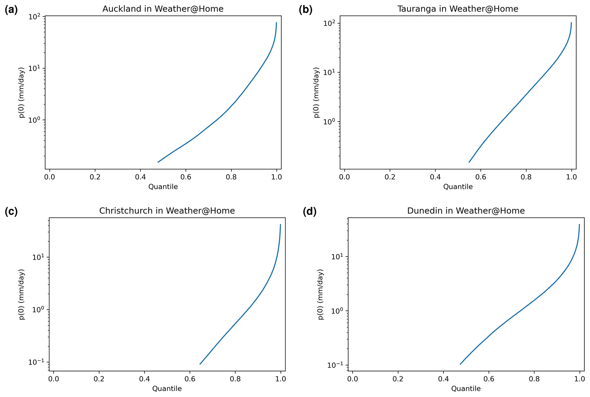
Figure 15 The p₀ values, i.e. the precipitation when $T_{\mathrm{SH}-\mathrm{land}}^{\prime }$ is zero (1765), derived from the weather@home HAPPI ensembles as a function of percentile.

5.3 Post hoc addition of non-stationarity

Here we consider an approach where, given a time series of hourly precipitation generated by the stationary SPG, a post hoc correction is applied to encapsulate non-stationarity in such a way that the SPG can be used to simulate expected future changes in precipitation. First, the three weather@home ensembles described in Sect. 2.4 were used to establish a relationship between precipitation and $T_{\mathrm{SH}-\mathrm{land}}^{\prime }$. The hourly precipitation time series simulated by the SPG were scaled to ensure that their correlation to $T_{\mathrm{SH}-\mathrm{land}}^{\prime }$ was the same as the correlation between the weather@home time series and $T_{\mathrm{SH}-\mathrm{land}}^{\prime }$ at each location. This scaling, detailed further below, was done independently across percentiles to avoid any potential biases between the weather@home data and the observed precipitation on which the SPG was trained. Each of the weather@home ensembles is associated with a specific $T_{\mathrm{SH}-\mathrm{land}}^{\prime }$ value (Table 5), and the mean precipitation within each ensemble, at each location, was analysed to extract the sensitivity of the precipitation to $T_{\mathrm{SH}-\mathrm{land}}^{\prime }$. Approximately 900 000 daily precipitation values were available for each site for each of the three values of $T_{\mathrm{SH}-\mathrm{land}}^{\prime }$.

An example of the fit of the equation described in Sect. 5.1 to extract this sensitivity is shown in Fig. 14, noting however that rather than showing the individual quantile values derived for each year across all ensemble members (noting that each member contributes a year of data), the ensemble mean is shown for clarity. In practice such fits are made to many thousands of values at each $T_{\mathrm{SH}-\mathrm{land}}^{\prime }$ value on the x axis of Fig. 14, and the uncertainty of that fit is what is shown in Figs. 11 to 13.

Because weather@home precipitation values below 0.1 mm d⁻¹ were omitted from this analysis as these were considered to be dry days, this often resulted in these sensitivities not being available below the 50th percentile.

The p₀ values derived from the equation fits within each percentile are shown in Fig. 15. Plots for all cities were very similar in shape. They all showed believable values for the quantile range, from about 0.1 to about 200 mm d⁻¹.

The rates/sensitivities of precipitation to $T_{\mathrm{SH}-\mathrm{land}}^{\prime }$ (in % K⁻¹) are plotted for each quantile in Fig. 16. While Auckland and Tauranga show drying tendencies for all but the highest percentiles of precipitation, for Christchurch and Dunedin the weather@home simulations suggest increases in precipitation across almost all percentiles with increases in $T_{\mathrm{SH}-\mathrm{land}}^{\prime }$.

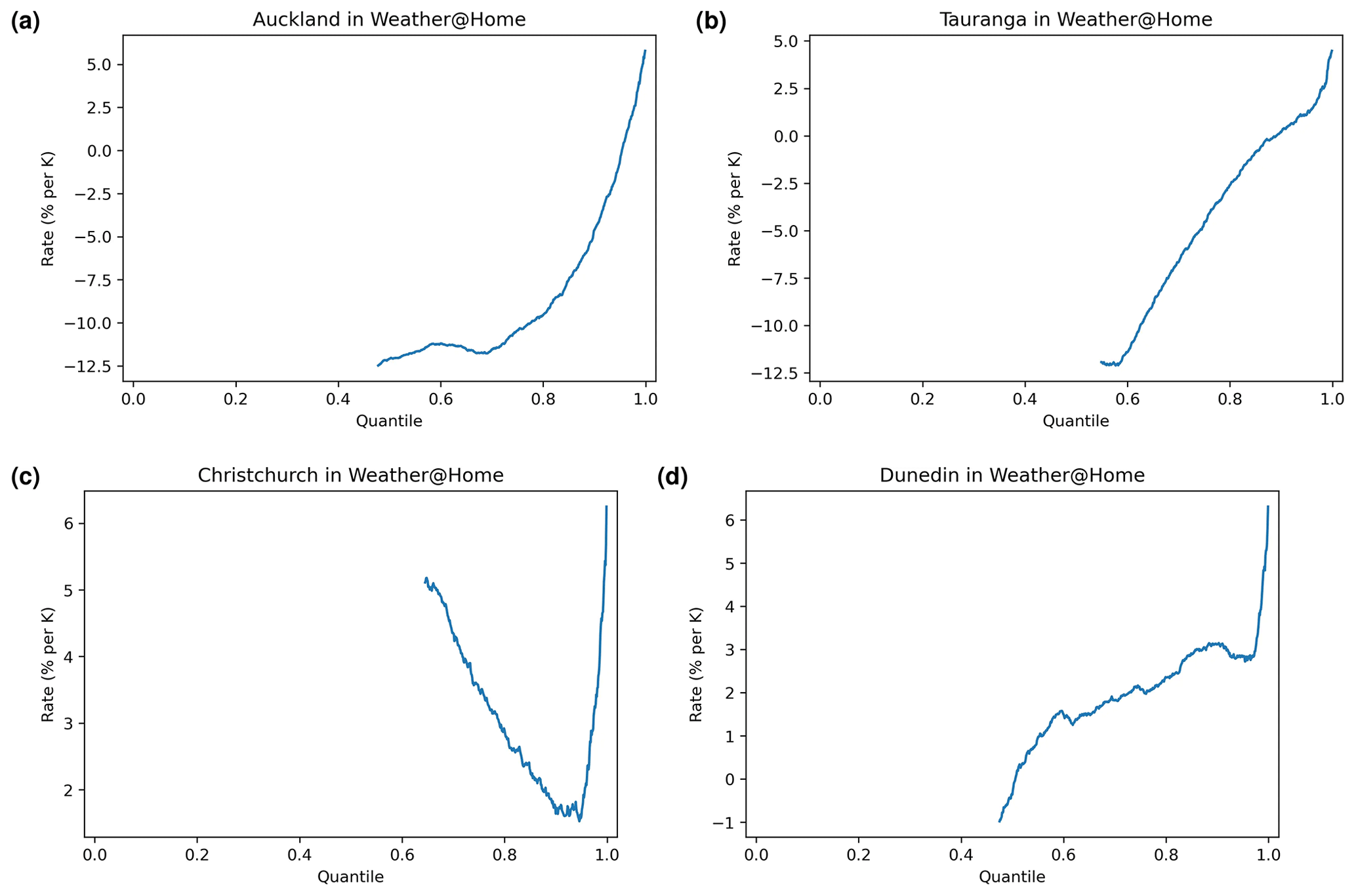
Figure 16 The sensitivities of precipitation (rates) to changes in $T_{\mathrm{SH}-\mathrm{land}}^{\prime }$, in percent per kelvin (% K⁻¹) and for each percentile, extracted from the weather@home simulations at each of the four cities.

To use the results presented in Fig. 16 to add non-stationarity to the hourly SPG, the time series generated by the SPG were first summed to daily time series to ensure temporal resolution alignment with the weather@home simulations. These daily resolution SPG time series were then indexed by $T_{\mathrm{SH}-\mathrm{land}}^{\prime }$. $T_{\mathrm{SH}-\mathrm{land}}^{\prime }$ anomalies were then calculated with respect to the period over which the hourly SPG was trained, hereafter referred to as Δx, based on the assumption the neural network's output was aligned with the average $T_{\mathrm{SH}-\mathrm{land}}^{\prime }$ value it saw during training. Each value in any daily SPG precipitation time series is then also indexed by its associated quantile. The associated rate for that quantile (Fig. 16) was then used to calculate a scaling for the precipitation as $\mathrm{1}+\frac{p\left(x_{\mathrm{2}}\right)-p\left(x_{\mathrm{1}}\right)}{p\left(x_{\mathrm{1}}\right)}=e^{r(x_{\mathrm{2}}-x_{\mathrm{1}})}=e^{r\mathrm{\Delta }x}$, where x₁ is the $T_{\mathrm{SH}-\mathrm{land}}^{\prime }$ mean over the training period and x₂ is the $T_{\mathrm{SH}-\mathrm{land}}^{\prime }$ value for the specified day in the non-stationary time series. The application of this scaling to the absolute hourly precipitation generated the non-stationary hourly precipitation. The utility of this post hoc approach is assessed in Sect. 5.4 below.

5.4 Post hoc addition results

An ensemble of hourly stationary SPG simulations, to which the post hoc non-stationarity correction described above was applied, were analysed for their sensitivity to $T_{\mathrm{SH}-\mathrm{land}}^{\prime }$. In total 110 ensembles were generated over the time period from 1980 to 2100, using the stationary hourly SPG for each location, which is of course invariant to $T_{\mathrm{SH}-\mathrm{land}}^{\prime }$ and therefore the year. For each of the RCP and SSP greenhouse gas emissions scenarios (RCP2.6, RCP4.5, RCP6.0, RCP8.5, SSP119, SSP126, SSP245, SSP370, SSP434, SSP460, SSP585), 10 of the ensembles were transformed using the post hoc non-stationary correction with the corresponding values of $T_{\mathrm{SH}-\mathrm{land}}^{\prime }$ from the scenario over the time period 1980 to 2100. These sensitivities of the transformed simulations are compared to those derived from the weather@home simulations in Fig. 17. The agreement between the sensitivities is very good, though this is not too surprising given that the post hoc transformations applied to the SPG hourly precipitation values were themselves derived from the weather@home simulations as described in Sect. 5.3. The agreement is not perfect since the multipliers, derived from daily precipitation, are applied to hourly values. These post hoc-corrected simulations show similar validation results to the stationary simulations presented in Sect. 4 (not shown).

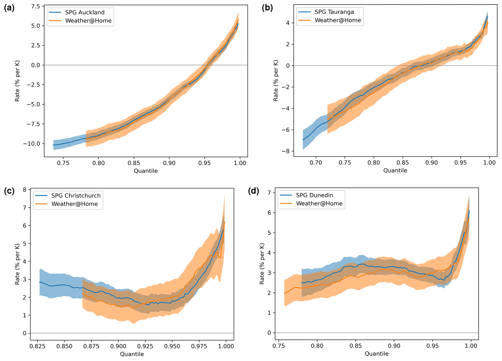
Figure 17 Rate of change of precipitation (% K⁻¹) by quantile for the post hoc-corrected SPG and the weather@home data set.

6 Discussion and conclusions

We have demonstrated the utility of a deep-neural-network-based mixture model as the basis for a single-site stochastic precipitation generator (SPG). Stationary versions of a daily and hourly resolution SPG were shown to generate precipitation time series that matched several key attributes derived from observed precipitation time series including the probability density of precipitation depth, the seasonal cycle in precipitation, the auto-correlation in precipitation, and the dry-period frequency.

Furthermore, it was shown that a neural network is capable of learning the non-stationarity in the precipitation from data, provided the climate signal in the data is strong and that the data are free of any inhomogeneities. Unfortunately, observational records are unlikely to meet these prerequisites such that attempting to learn the non-stationarity from observational records and projecting that non-stationarity outside of the training domain is likely to lead to unreliable projections of expected future changes in precipitation. To ameliorate such deficiencies in our non-stationary SPGs a post hoc correction was developed using sensitivities of precipitation to $T_{\mathrm{SH}-\mathrm{land}}^{\prime }$ derived from weather@home simulations (a regional climate model) to create daily and hourly non-stationary SPGs suitable for projecting expected changes in precipitation into the future.

While the SPGs presented here are significantly computationally faster (by many orders of magnitude) than typical regional climate models (RCMs), they should not be seen as universal alternatives to climate models – the SPG simulations of expected changes in precipitation over the near future (next 2–3 decades) are likely to be robust as the climate of the next few decades is unlikely to be significantly different from that of the last century on which the SPGs were trained. Non-linearities in the climate system, absent in the historical record on which the SPGs were trained, may be adequately simulated by RCMs which encapsulate much of our understanding of the physics of the climate system but are very unlikely to be well simulated by the SPGs since the SPGs had no opportunity to learn of these non-linearities. We also emphasize that the SPGs presented here are single-site SPGs, and simulated precipitation time series from two nearby sites will lack the temporal correlation observed in reality and simulated by RCMs; i.e. the spatial morphology of precipitation fields cannot be simulated by these SPGs. That said, these SPGs have several advantages over RCMs, the main being their ability to generate very large ensembles of simulations for a wide range of future greenhouse gas emissions scenarios, including simulating events that were not seen in the training data set. This would include many rare but extreme precipitation events sufficient to describe potential changes in their frequency or severity with a statistical robustness that would not be achievable with a small ensemble of RCM simulations. Our intention is to use these SPGs to simulate hourly precipitation time series with the SPGs, for the next few decades, with a view to quantifying the impacts of expected changes in the frequency and severity of extreme precipitation events at selected single sites.