Improving Antarctic Bottom Water precursors in NEMO for climate applications

The world's largest ice shelves are found in the Antarctic Weddell Sea and Ross Sea where complex interactions between the atmosphere, sea ice, ice shelves and ocean transform shelf waters into High Salinity Shelf Water (HSSW) and Ice Shelf Water (ISW), the parent waters of Antarctic Bottom Water (AABW). This process feeds the lower limb of the global overturning circulation as AABW, the world's densest and deepest water mass, spreads outwards from Antarctica. None of the coupled climate models contributing to CMIP6 directly simulated ocean–ice shelf interactions, thereby omitting a potentially critical piece of the climate puzzle. As a first step towards better representing these processes in a global ocean model, we run a 1^∘ resolution Nucleus for European Modelling of the Ocean (NEMO; eORCA1) forced configuration to explicitly simulate circulation beneath the Filchner-Ronne Ice Shelf (FRIS), Larsen C Ice Shelf (LCIS) and Ross Ice Shelf (RIS). These locations are thought to supply the majority of the source waters for AABW, and so melt in all other cavities is provisionally prescribed. Results show that the grid resolution of 1^∘ is sufficient to produce melt rate patterns and total melt fluxes of FRIS (117 ± 21 Gt yr⁻¹), LCIS (36 ± 7 Gt yr⁻¹) and RIS (112 ± 22 Gt yr⁻¹) that agree well with both high-resolution models and satellite measurements. Most notably, allowing sub-ice shelf circulation reduces salinity biases (0.1 psu), produces the previously unresolved water mass ISW and re-organizes the shelf circulation to bring the regional model hydrography closer to observations. A change in AABW within the Weddell Sea and the Ross Sea towards colder, fresher values is identified, but the magnitude is limited by the absence of a realistic overflow. This study presents a NEMO configuration that can be used for climate applications with improved realism of the Antarctic continental shelf circulation and a better representation of the precursors of AABW.

1 Introduction

The Southern Ocean plays a vital role in global ocean circulation and in the storage of both heat and carbon (Marshall and Speer, 2012; Frölicher et al., 2015; Rintoul, 2018). Within this backdrop, the processes taking place adjacent to and underneath the Antarctic ice shelves are not only important for controlling regional ocean dynamics but also for facilitating globally important water mass transformations (Schodlok et al., 2016). Sea ice formation on the continental shelf decreases the buoyancy of the underlying waters through the process of brine rejection creating High Salinity Shelf Water (HSSW; Jacobs et al., 1979). When this dense water mass is formed adjacent to an ice shelf, it can follow deep bathymetric pathways into the neighbouring sub-ice shelf cavity and interact with the base of the ice to form Ice Shelf Water (ISW; Jenkins, 1991). These dense waters then accumulate on the continental shelf and migrate towards the shelf break to cascade down the continental slope as a gravity current (Gordon, 1986; Whitehead, 1987). As the waters descend towards the depths, they mix with and entrain ambient water masses until they reach either a density neutral depth, or the sea floor, at which point they spread outwards as Antarctic Bottom Water (AABW) (Bergamasco et al., 2003; Huthnance, 1995). AABW plays a crucial role in the global overturning circulation, in abyssal ventilation and in the cross-basin transport of heat, salt, carbon, nutrients and numerous other tracers (Killworth, 1983; Johnson, 2008; Orsi, 2010). The principal locations for the formation of the source waters of AABW are the Weddell Sea and Ross Sea, adjacent to the large ice shelves (Orsi et al., 1999; van Caspel et al., 2015; Kerr et al., 2018; Bowen et al., 2021).

Filchner-Ronne Ice Shelf (FRIS) is located at the southern boundary of the Weddell Sea and represents 28 % of the total Antarctic ice shelf area (Fig. 1a). Traditionally FRIS has been viewed as having the greatest contribution to AABW by forming the coldest and most oxygen-rich dense waters in the Southern Ocean (Nicholls et al., 2009; Naveira Garabato et al., 2002). Observations for the southern Weddell Sea continental shelf indicate that HSSW enters the FRIS cavity following the Ronne Depression (Fig. 1a), circulates under the cavity causing melting at the base of the ice shelf at great water pressures and then exits as colder and fresher ISW via the Filchner Trough (Nicholls et al., 2001, 2004; Janout et al., 2021). This outflowing ISW mixes with HSSW formed on the shallow continental shelf adjacent to Berkner Island and cascades down the continental slope, mixing with ambient modified Circumpolar Deep Water (CDW) to form AABW (Fahrbach et al., 1995; Nicholls et al., 2009).

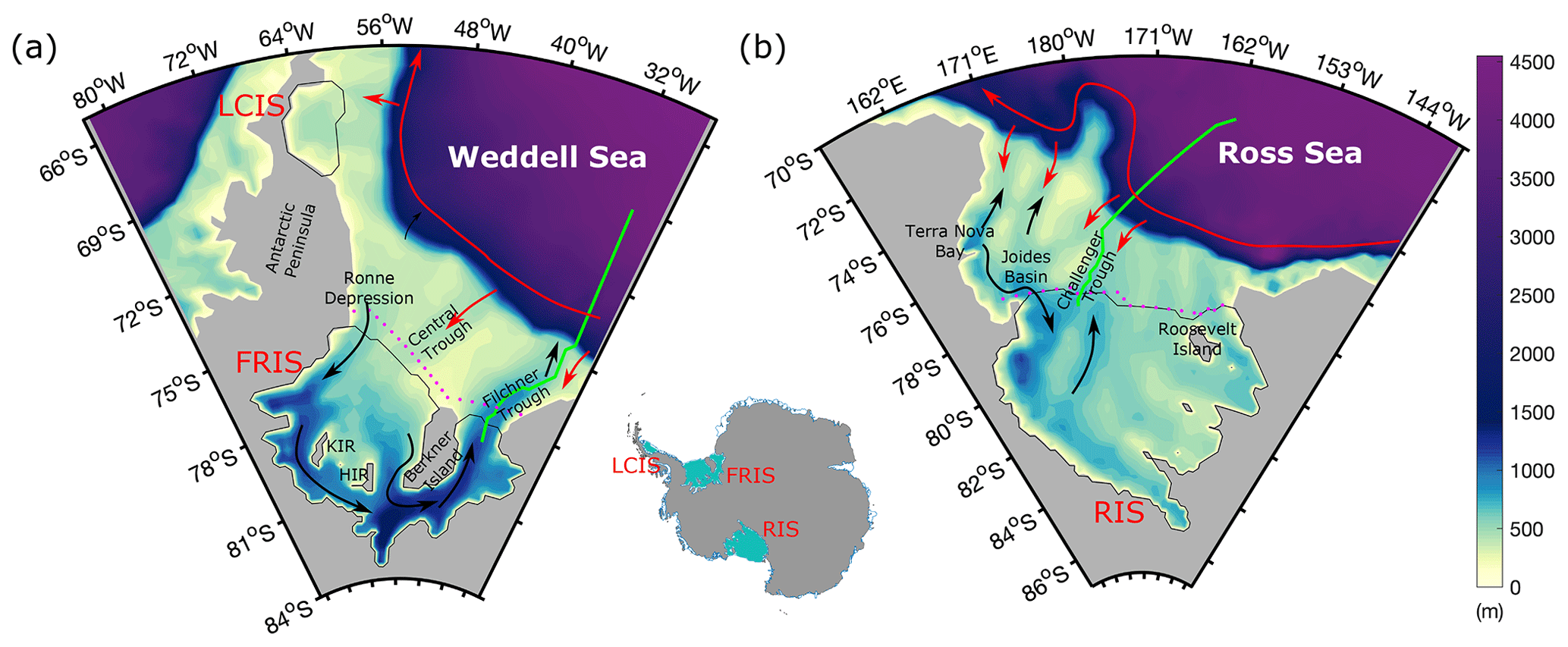
Figure 1 Model bathymetry for (a) the Weddell Sea and (b) the Ross Sea with main topographic features labelled (KIR – Korff Ice Rise and HIR – Henry Ice Rise). Red arrows show direction of flow of warm deep water, and black arrows indicate dense shelf water circulation according to observational estimates. Circulation features depicted in this figure are adapted from information presented in Budillon et al. (2003), Bergamasco et al. (2003), Russo et al. (2011) and Janout et al. (2021). Dotted magenta lines indicate sections used for CTD comparisons, and green lines show shelf cross sections used for analysis in Figs. 6 and 7.

While the main formation site of the source waters of AABW in the Weddell Sea is the FRIS continental shelf, Larsen C Ice Shelf (LCIS) is also thought to play an important role. Nestled into the arc of the Antarctic Peninsula (Fig. 1a), processes adjacent to this ice shelf produce a fresher variety of dense water called Weddell Sea Deep Water (WSDW), which is lighter than the Weddell Sea Bottom Water (WSBW) formed further south (Fahrbach et al., 1995; Gordon et al., 2001). This water mass is less hindered by bathymetric constraints so that it is more easily transported out of the gyre over the South Scotia Ridge to make an important contribution to AABW (Abrahamsen et al., 2019; van Caspel et al., 2015).

The Ross Sea, the second largest site for AABW formation, is home to Antarctica's largest ice shelf, representing 32 % of the total Antarctic ice shelf area (Rignot et al., 2013). The Ross Ice Shelf (RIS) is located at the southern boundary of the Ross Sea (Fig. 1b) where the continental shelf has very irregular topography with numerous troughs and depressions that act as reservoirs for dense waters (Budillon et al., 2003). Just offshore, CDW flows largely un-modified within the Ross Gyre and mixes with the local waters at the shelf break (Fig. 1b), providing a source of heat and making this a region of dynamic water mass exchange (Bergamasco et al., 2003; Budillon et al., 2003). Two recurring ice-free zones are the principal formation sites for HSSW in the area: one located at the southwestern corner of the Ross Sea called the Terra Nova Bay polynya and another in front of RIS called the Ross Sea Polynya. This HSSW then spreads both northwards towards the shelf break and southwards under RIS (Fig. 1b). Similarly to FRIS, the HSSW flowing into the RIS cavity interacts with the base of the ice shelf to form ISW (Jacobs et al., 1979).

While freshwater input to the ocean from ice shelf melt is (at present) relatively small in magnitude, it exerts a strong modulating effect on dense water formation and Southern Ocean water mass transformation (Schodlok et al., 2016; Jeong et al., 2020). The impacts of increased meltwater in a warming climate could, in addition to raising sea level, actually reduce AABW formation with major consequences for global overturning (Silvano et al., 2018; Williams et al., 2016). One possible series of events common to simulations by the E3SM, CSIRO Mk3L and LOVECLIM climate models describes how surface freshening from ice shelf melt would increase stratification along the Antarctic coast, inhibit full depth convection and the formation of dense shelf water, and simultaneously trap warm water at depth, resulting in further ice shelf melting and a horizontal propagation of the warming signal (Jeong et al., 2020; Phipps et al., 2016; Menviel et al., 2010).

Despite the importance of ocean–ice shelf interactions for the climate system, none of the models contributing to the DECK experiments of the Coupled Model Intercomparison Project Phase 6 (CMIP6; used to inform the Intergovernmental Panel on Climate Change (IPCC) Sixth Assessment Report (AR6)) explicitly represented circulation within sub-ice shelf cavities (Heuzé, 2021). This has lowered confidence in projected trends for the Southern Ocean and has limited our ability to incorporate the impacts of global ocean warming on the Antarctic Ice Sheet (Meredith et al., 2019; Beadling et al., 2020; Comeau et al., 2022). In most coupled climate models, the formation of dense water is poorly represented as AABW is formed via open-ocean convection, often with mixed layers that are too deep and polynyas that are too large and too frequent (Heuzé et al., 2013; Mohrmann et al., 2021). In reality, deep open-ocean convection events able to produce AABW are rarely observed (Goosse et al., 2021), and instead ocean–sea ice–atmosphere interactions adjacent to the Antarctic ice shelves are responsible for the creation of the majority of AABW source waters.

The authors propose that the path towards improving AABW realism in coupled climate models starts with a more accurate simulation of the dense precursors on the Antarctic continental shelf. Then, work needs to be done on improving the overflows so as to facilitate the downslope export of these waters and on decreasing the strength of open-ocean convection (Heuzé, 2021). The Nucleus for European Modelling of the Ocean (NEMO) model is used as the ocean component in many climate models (Hazeleger et al., 2010; Scoccimarro et al., 2011; Hewitt et al., 2011, 2016; Dufresne et al., 2013; Voldoire et al., 2013; Cao et al., 2018; Swart et al., 2019), and consequently the development of configurations with improved realism of Antarctic shelf water circulation and AABW source water properties is of interest to a large community.

Ice shelf melt has previously been represented using NEMO in a variety of ways: prescribed using a freshwater flux at the surface, a fixed flux distributed over the depth range of the mouth of the ice shelf front, a specified melt at the base of the ice shelf, and an interactive melt with both fixed geometry and evolving coupled ice shelves (Mathiot et al., 2017; Storkey et al., 2018; Smith et al., 2021). The simulations with a fixed freshwater flux parameterization at depth perform well in terms of mimicking the vertical overturning and associated entrainment of ice shelf melt but do not allow for interactive ice–ocean exchange that evolves with ocean properties. Parameterizations of ice shelf melt using far field temperature (outside of the cavities) exist, and an extensive comparison was undertaken in Burgard et al. (2022). Here they found that none of the available parameterizations yield a negligible error, and so parameterizing basal melt still remains a challenge. Furthermore, these parameterizations do not solve the need to allow for circulation underneath the ice shelves in order to produce the horizontal variability observed on the continental shelf. For this, it is necessary to open the sub-ice shelf cavities in the simulation (Mathiot et al., 2017; Storkey et al., 2018; Comeau et al., 2022). Of all the previous studies using NEMO configurations with explicit sub-ice shelf cavities, only one has been at a resolution that is compatible with long-term climate projection applications, that developed by Smith et al. (2021) where a global ocean 1^∘ NEMO (eORCA1) is coupled with interactive ice sheets in the U.K. Earth System model (UKESM). Previous studies have proven very useful in illustrating the strengths and weaknesses of NEMO's representation of ocean–ice shelf interactions, but the results apply to regional configurations (e.g. Mathiot et al., 2017; Jourdain et al., 2017; Hausmann et al., 2020; Huot et al., 2021) or high-resolution global configurations (e.g. $\mathrm{1}/\mathrm{4}$ and $\mathrm{1}/\mathrm{12}$^∘ in Storkey et al., 2018) and so do not fit the needs of typical CMIP models. The results presented by Smith et al. (2021) for UKESM with NEMO eORCA1 coupled to an Antarctic ice sheet model highlight the substantial advancement in model development but do not show how this coupling affects the realism of Southern Ocean water mass properties and dynamics. Evaluation of the initial state of the UKESM (NEMO coupled to BICYCLES ice sheet model) was undertaken by Siahaan et al. (2022), but the investigation served to check for the absence of large biases, and so an in-depth comparison was not carried out.

A gap therefore exists to take a step-by-step approach to represent ice shelf–ocean interactions in NEMO for climate applications. Additionally, a well-documented description of one possible method to simulate sub-ice shelf cavity circulation in low-resolution ocean models could be of use in the designing of the next phase of CMIP. In this study we present the first proposed step in this journey by explicitly simulating circulation under only RIS, FRIS and LCIS. These ice shelves were chosen due to their direct role in the formation of the parent waters of AABW (Kerr et al., 2018; Bowen et al., 2021) and due to their large size and thus practicality of realistically simulating their sub-ice shelf cavities in a global ocean 1^∘ setup. We choose to keep all other ice shelf cavities closed with prescribed melt rates injected at the mouth of the front using the method described by Mathiot et al. (2017). This includes the relatively large Amery Ice Shelf cavity, despite its role in preconditioning bottom water formation in the Cape Darnley polynya (Williams et al., 2016) because this polynya is absent in our configuration (due to the absence of icebergs and landfast sea ice). We choose to explore the changes in circulation, melt rates and water mass properties in the Weddell Sea and the Ross Sea in a forced scenario with fixed cavity geometry, as coupling can introduce further biases and obscure the changes attributed to sub-ice shelf circulation. By taking this circumspect approach, it is possible to diagnose the impact of ocean–ice shelf interactions on the parent waters of AABW and produce a validated configuration of NEMO that can either be used for the next generation of climate models or as an interim step towards dynamic ice-sheet coupling.

The model setup, configurations used in this study, forcing, and methodology to establish initial conditions under the ice shelves are described in Sect. 2. A validation of the reference configuration compared to ocean observations is presented in Sect. 3. Section 4 then explores the results from the “open” cavity simulation and compares melt rates and thermohaline properties with other model estimates and observed values. Section 5 provides the reader with a summary discussion, and Sect. 6 presents a conclusion of the findings of this study. Additional information regarding model namelist nomenclature, representation of tides, an investigation into sea ice production, and plots showing AABW volume and bottom density changes are provided in the Supplement.

2 Methods

2.1 Model setup

For this study, we use version 4.2 of NEMO (NEMO System Team, 2022). NEMO is a three-dimensional, free-surface, hydrostatic, primitive-equation global ocean general circulation model. Our configuration uses the eORCA1 global grid, with a nominal horizontal resolution of 1^∘ at the Equator and a reduction in meridional grid spacing towards higher latitudes to match the accompanying shrinking of the zonal dimension of the grid cells. In the Southern Hemisphere, the model grid has been extended to reach 85^∘ S to allow for the representation of the sub-ice shelf seas according to the procedure described in Mathiot et al. (2017). The average horizontal resolution of the grid under RIS, FRIS and LCIS is 20, 22 and 42 km respectively. To account for the decrease in the horizontal size of grid cells at high latitudes, we decide to linearly scale the Laplacian eddy viscosity south of 65^∘ S according to grid cell size. In the vertical, the configuration possesses 75 levels, with thickness increasing from 1 m at the surface to 200 m at depth (Storkey et al., 2018). We use the z^* vertical coordinate adapted to the ice shelf so that all cells between the surface and the ice shelf base are masked at initialization and the effect of the ice shelf on friction and pressure gradient is calculated (Madec and NEMO System Team, 2019; Mathiot et al., 2017). The bathymetry used is derived from the Earth TOPOgraphy version 2 dataset (ETOPO2v2; NOAA, 2006) with information for the extension under the ice shelves based on the International Bathymetric Chart of the Southern Ocean (IBSCO; Arndt et al., 2013). For the calculation of the thermodynamic properties of seawater, NEMO uses the Thermodynamic Equation Of Seawater – 2010 (TEOS-10), giving results in conservative temperature and absolute salinity, which, for the purposes of this study, were converted to potential temperature and practical salinity in order to facilitate comparison of the model results with observations and known signatures of water masses. For more information regarding the choices of advection and diffusion schemes, mixing coefficients and eddy parameterizations, please refer to the copy of the namelists provided in the accompanying data repository. A note explaining the nomenclature of the namelists and the differences between the open and “closed” cavity simulations can be found in the Supplement Sect. S1.

The effect of tides on vertical mixing (through breaking of internal waves) is taken into account in NEMO using the energy constrained parameterization of de Lavergne et al. (2020). This mixing parameterization does not, however, represent trapped waves at high latitudes or any tide-induced internal-wave mixing below ice shelves and does not include the effect of tides on basal friction and thus melting of the ice shelves. To address this, by default there is a parameter (rn_ke0) representing the background kinetic energy associated with tides which is set to a constant of $\mathrm{2.5}\times {\mathrm{10}}^{-\mathrm{3}}$ m² s⁻² everywhere. We tested another methodology of parameterizing the impact of tides on melting according to Jourdain et al. (2019) using CATS2008 two-dimensional tidal velocities; as summarized in the Supplement Sect. S2 and Fig. S1, this alternative parameterization brings marginal changes in the simulated melt patterns and bulk melt rates (< 10 %). The explicit representation of tides is not advisable in a configuration designed for climate applications due to the high levels of numerical mixing induced.

The ocean dynamics component, NEMO OCE, is coupled with SI³, the dynamic and thermodynamic sea ice model of NEMO (Rousset et al., 2015; Vancoppenolle et al., 2023). SI³ is directly resolved on the ocean grid, based on an energy- and salt-conserving approach for sea ice thermodynamics (Vancoppenolle et al., 2023), multiple categories to resolve subgrid-scale variations in ice thickness (Bitz et al., 2001; Lipscomb, 2001), a second-order-moment-conserving scheme for horizontal advection (Prather, 1986), and the adaptive elastic–viscous–plastic formulation for the rheology term of the momentum equation (Kimmritz et al., 2016).

2.2 Open vs closed configurations

Here, we present results from two configurations: first a closed-cavity reference configuration, where ice shelf melt is prescribed in a way that mimics the ice-shelf overturning, and secondly an open-cavity configuration. For the reference closed-cavity configuration, a fixed freshwater flux corresponding to the volume of basal meltwater estimated by Depoorter et al. (2013) for each ice shelf is added into the ocean evenly between the ocean floor and the base of the ice shelf, horizontally uniform across the ice shelf front, and a vertical wall closes the cavity at this location (as in Mathiot et al., 2017). The fixed freshwater flux is based on Depoorter et al. (2013) melt estimates as this is the same file used for the IPSL climate model. Furthermore, the ice shelf area surveyed by Adusumilli et al. (2020) only extends to 81.5^∘ S so that RIS and FRIS are not fully covered and therefore do not have the full melt flux. For the open-cavity configuration, the majority of ice shelves are kept closed using the same method as described above, and only three of the largest cold water ice shelves are opened. Circulation is simulated under RIS, FRIS and LCIS where the prescribed freshwater flux is turned off at the mouths of these cavities and interactive melt is activated. Ice shelf melt and freeze are calculated using the three-equation formulation (Hellmer and Olbers, 1989; Holland and Jenkins, 1999; Asay-Davis et al., 2016) in which the temperature, salinity and velocities are averaged over a fixed boundary layer thickness of 30 m chosen according to Losch (2008). The top drag coefficient used is 10⁻³, and the temperature and salinity transfer coefficients used are $\mathrm{1.4}\times {\mathrm{10}}^{-\mathrm{2}}$ and $\mathrm{4}\times {\mathrm{10}}^{-\mathrm{4}}$ respectively. Note that a fixed ice shelf geometry is maintained, thereby assuming a steady state where all ice melted by the ocean is replaced by the seaward advection of new ice (Schodlok et al., 2016; Mathiot et al., 2017).

By using this combination of explicit and parameterized ice shelf cavities, we provide an intermediate step between prescribed melt and explicit cavities or even ice sheet coupling and gain experience and a better understanding of the impact on ocean dynamics in order to better inform future choices. The advantage of this approach is that it allows us to specify the melt for small cavities which remain unresolved or insufficiently resolved at a 1^∘ resolution and simultaneously utilize the model capability to resolve sub-ice shelf cavity circulation under the large, cold ice shelves, which allows for more realistic formation of the source waters of AABW. In terms of computing cost, the open-cavity configuration costs 11 % more than the closed-cavity simulation (mostly due to addition of cells as the model grid is extended further south; only 0.3 % of this is associated with the cost of the ice shelf routines themselves). Figure 1 shows the extended bathymetry of eORCA1 for the Weddell Sea and the Ross Sea, with the three ice shelf cavities of interest un-masked and important features labelled.

2.3 Forcing

For both open and closed configurations, the model was run for 124 years using two cycles of interannual (1948–2009) CORE forcing (Coordinated Ocean-ice Reference Experiments version 2; Large and Yeager, 2004; Griffies et al., 2009). Sea surface salinity restoring is activated but not under sea ice as we have low confidence in the sea surface salinity climatology in this area due to limited observations. Freshwater discharge from iceberg melt is parameterized using a prescribed surface flux with realistic distribution (Merino et al., 2016), based on calving estimates from Depoorter et al. (2013).

2.4 Initial conditions

For all simulations, global ocean properties were initialized using the 1981–2010 climatology of World Ocean Atlas 2013 (WOA2013; Locarnini et al., 2013; Zweng et al., 2013) as this dataset is used for the IPSL climate model and so was a convenient choice. This climatology does not, however, extend under the Antarctic ice shelves, and so in order to provide somewhat realistic initial conditions underneath FRIS, LCIS and RIS, we employed an idealized regional configuration of each ice shelf. For this we created a NEMO test case using a closed domain, with temperature and salinity restoring at the boundaries; 75 vertical layers; and a resolution, time step and bathymetry corresponding to those of eORCA1. The domain for each of the 3 configurations included just the ice shelf and adjacent continental shelf and slope and so were reasonably low-cost and fast to run in order to perform sensitivity experiments. The simulations were initialized with a constant and uniform temperature and salinity and restored at the boundaries using a mean profile from WOA2013 for that region. The choices for initial thermohaline properties inside the cavities were informed by calculating the mean values of detected ISW from CTD (conductivity, temperature, and depth) observations performed in the area adjacent to each ice shelf and converting these to conservative temperature and absolute salinity for input to the model (−2 ^∘C and 34.76 for FRIS (Janout et al., 2021), −1.95 ^∘C and 34.74 for LCIS (Nicholls et al., 2004; Hutchinson et al., 2020), and −1.94 ^∘C and 34.76 for RIS (Bergamasco et al., 2003; Budillon et al., 2003)). Each simulation was run for 10 years, which was found to be sufficiently long to spin up the circulation within each cavity and reach a stable melt rate. The temperature–salinity distributions within the cavity were extracted and merged with WOA2013 data re-gridded to the NEMO eORCA1 grid, with a cubic spline used to smooth the data discontinuity across the ice shelf front. By following this method we have attempted to provide as realistic initial conditions for eORCA1 as possible, with the simulation starting with CORE forcing from the 1 January 1948.

3 Water mass realism in NEMO without cavities

To assess the existing biases in the representation of dense water properties in NEMO v4.2 eORCA1 standard configuration (closed), full depth temperature versus salinity plots along with bottom temperature and salinity are compared with World Ocean Atlas (WOA 2018) gridded observations from 1981–2010 (Locarnini et al., 2018; Zweng et al., 2019) in Figs. 2 and 3 for the Weddell Sea and the Ross Sea respectively.

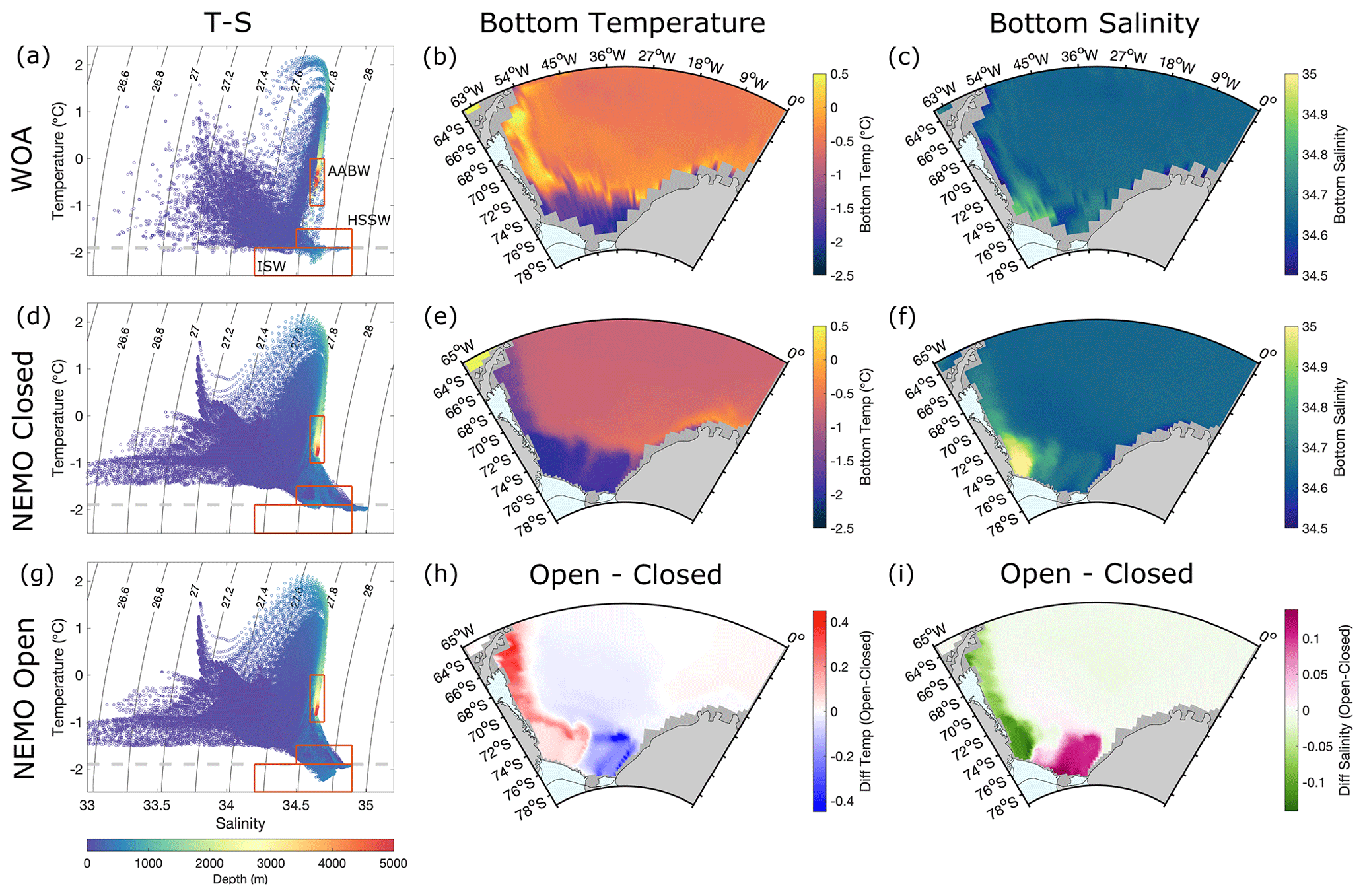
Figure 2 Weddell Sea comparison of NEMO v4.2 eORCA1 reference configuration (closed; d–f) for equivalent years 1981–2009 to be compared with World Ocean Atlas (WOA; Locarnini et al., 2018; Zweng et al., 2019) observational dataset (a–c). The temperature–salinity distributions in density space are shown in plots (a), (d) and (g), with the dashed grey line representing surface freezing point and labels in plot (a) indicating the observed ranges for properties corresponding to Antarctic Bottom Water (AABW), High Salinity Shelf Water (HSSW) and Ice Shelf Water (ISW) (Robertson et al., 2002; Hutchinson et al., 2020). Panels (b), (c), (e) and (f) show bottom temperature and salinity of WOA and the closed-cavity simulation, and the difference in bottom properties between the open- and closed-cavity configurations (open−closed) is shown in panels (h) and (i). Panels (a) and (g) exclude ice shelf cavity data matching the closed configuration of panel (d).

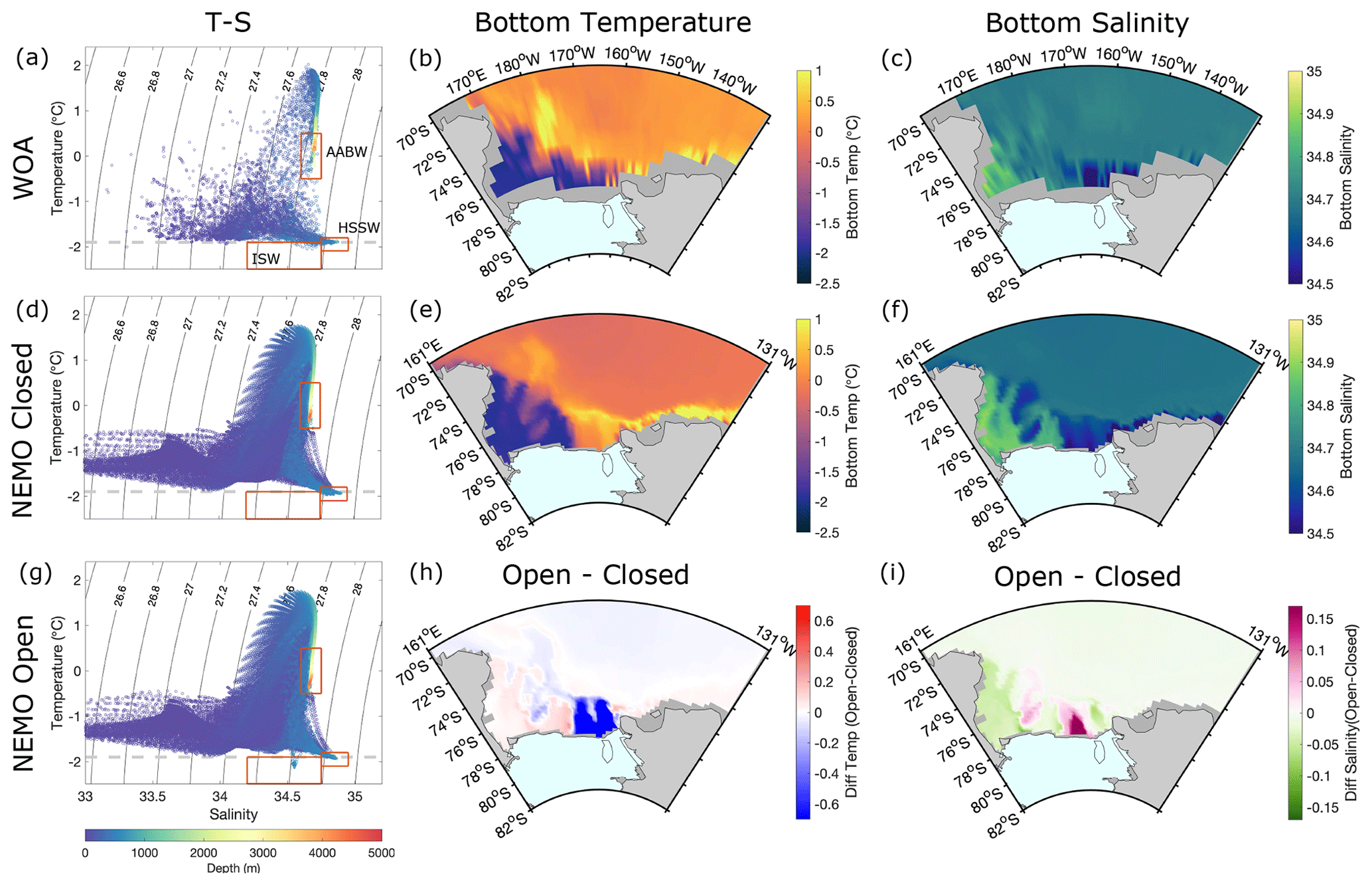
Figure 3 Same as Fig. 2 but for the Ross Sea.

WOA observations indicate the presence of HSSW on the southwestern continental shelf of the Weddell Sea, possessing salinities of up to 34.9 psu, likely sourced from the coastal polynya along the western flank of FRIS ice shelf front (Supplement Fig. S2a). On the eastern side of the FRIS ice shelf front, evidence of ISW can be seen with temperatures below surface freezing point (−1.9 ^∘C) and fresher salinities of around 34.65 psu (Fig. 2b and c). Results from CTD observations obtained on the continental shelf in front of FRIS propose an anticlockwise circulation pattern, with HSSW entering the cavity via the Ronne Depression and ISW exiting via the Filchner Trough (Fig. 1a; Janout et al., 2021). By comparison, the standard model configuration is overall too salty on the continental shelf, with HSSW properties that are out of the bounds of the observed range (HSSW box Fig. 2d). Most notably, there is a pool of HSSW that has built up in the Ronne Depression resulting in overestimations of bottom salinity and exaggerated cool conditions on the southwestern Weddell shelf (Fig. 2e and f). In terms of ISW, there is none detected in the model output (ISW box Fig. 2d), as in this configuration there is no explicit ocean–ice shelf interaction. Offshore bottom temperature is overall colder than in WOA, resulting in a core AABW signature that is at the lower limit of observed values (Fig. 2d). This is indicative of the effects of strong open-ocean deep convection (Heuzé, 2021), which is discussed further in Sect. 4.4.

Due to the limited observations adjacent to LCIS, WOA bottom properties do not capture the cold water masses located on the continental shelf detected by Hutchinson et al. (2020), where bottom temperatures of below −2 ^∘C and salinities of 34.6 psu were reported. Instead, Fig. 2b indicates very warm conditions (temperatures of around 0.5 ^∘C) on the western flank of the Weddell Sea. The authors explored the bottom properties in this area in the Southern Ocean State Estimate (SOSE; Mazloff et al., 2010) atlas and found bottom temperatures on the shelf adjacent to LCIS in line with those reported from hydrographic observations (−2 ^∘C), but the bottom salinities were found to be far too fresh (34.5 psu). A fair comparison can therefore not be realistically made between NEMO and an atlas for the area adjacent to LCIS, but by comparing the model output with the CTD results from Hutchinson et al. (2020; their Fig. 3b), we find the closed configuration to be too saline, with bottom salinities (34.8 psu) greater than those observed. The overly saline conditions along the western flank of the Weddell Sea are likely a spill-over effect from the HSSW buildup seen in the Ronne Depression further south (Fig. 2f).

WOA bottom temperatures and salinities for the Ross Sea indicate a strong east–west gradient in properties across the continental shelf (Fig. 3b and c). Conditions in the southwest reveal the cold and salty signature of HSSW likely formed in the Terra Nova Bay polynya and the Ross Polynya. Intrusions of CDW at the eastern portion of the RIS front can be seen by warm signatures of up to 1 ^∘C (Fig. 3b) and fresher bottom salinities (Fig. 3c). Hydrological and current meter data presented by Budillon et al. (2003) reported that HSSW dominates bottom properties within the troughs connected to the Joides Basin, and ISW dominates in the Challenger Trough (see locations of bathymetric features in Fig. 1b), thus indicating a western intensified anticlockwise circulation cell under RIS. In terms of HSSW properties, the model is within the observed range (Fig. 3d), yet the proportion and salinity of HSSW in Terra Nova Bay and Joides Basin appear to be overestimated (Fig. 3f). The bottom temperatures from NEMO indicate the presence of very warm waters, likely of circumpolar origin right on the eastern continental shelf (Fig. 3e), whereas in observations this shelf is found to be cold and the warm water confined offshore of the shelf break with only occasional intrusions (Bergamasco et al., 2003; Fig. 3b). Again, there is no ISW in this standard configuration, as there is no explicit model representation of ice shelf–ocean interactions. Offshore bottom properties are slightly cooler than WOA in the model, but the AABW signature (AABW box Fig. 3d) falls within the range reported from observations (Bergamasco et al., 2002; Budillon et al., 2003; Silvano et al., 2016).

4 Impact of explicit sub-ice shelf circulation

The following sections present results pertaining to the open-cavity run where the eORCA1 grid is extended under FRIS, LCIS and RIS to allow for circulation within the cavities and explicit interaction with the base of these ice shelves.

4.1 Melt rates

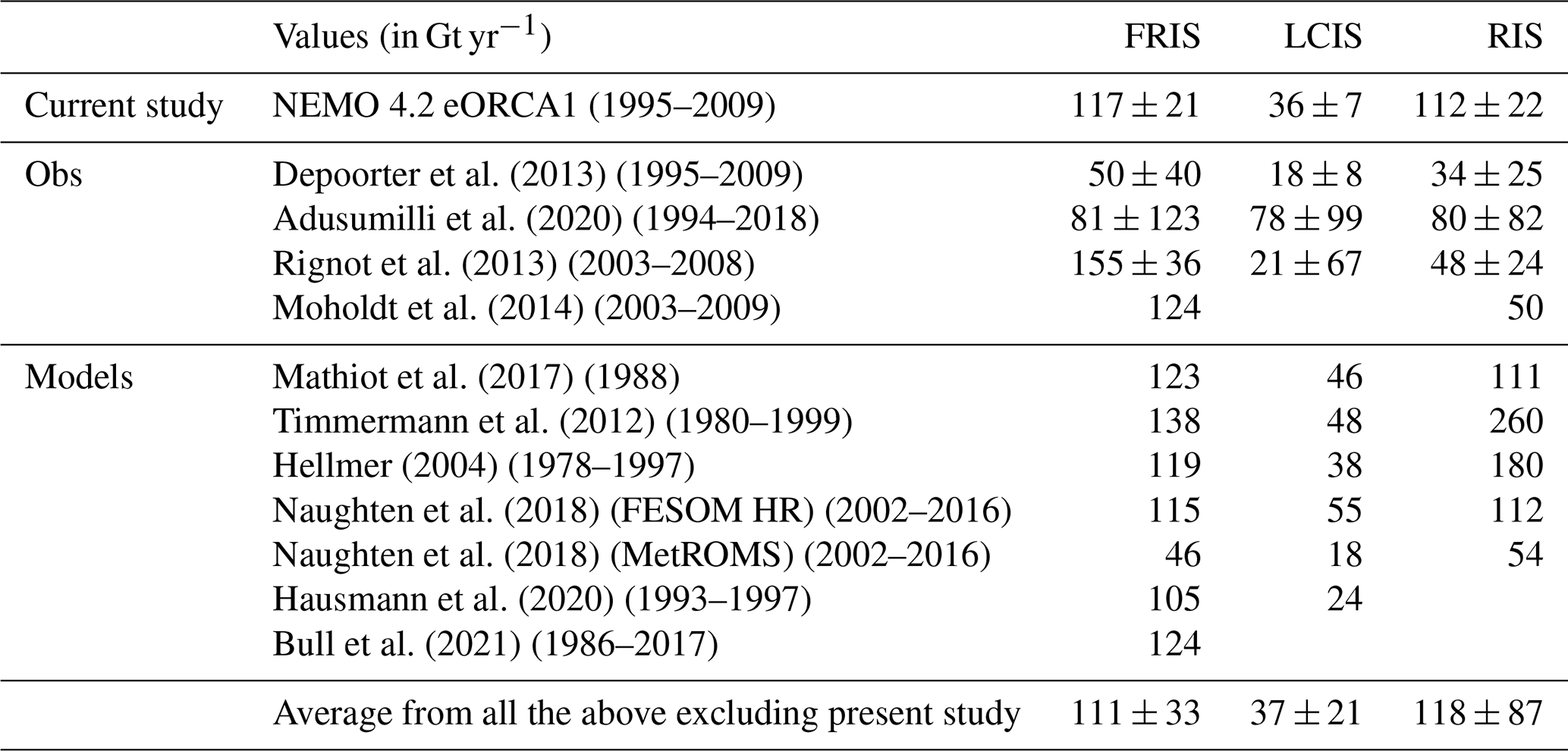
The average ice shelf melt rate pattern for FRIS, LCIS and RIS is shown in Fig. 4 for the model simulation equivalent years 1995 to 2009, where orange indicates melt and purple shows refreezing. The average total melt flux for this time period is shown in Table 1 and compared to Depoorter et al. (2013) from which the volumes for the prescribed melt were taken for the reference configuration (closed). Opening the cavities results in at least double the melt reported from Depoorter et al. (2013). This discrepancy reflects both a warm bias on the continental shelf in NEMO (Sect. 4.4) and a possible bias in Depoorter's estimates which are lower than all other satellite estimates (Table 1). The total melt fluxes of each ice shelf from various other observational and model studies are also listed in the table, showing the wide spread in basal melt estimates both within values calculated from observations and between observations and models (Table 1). The model studies of Mathiot et al. (2017) and Bull et al. (2021), which are both regional NEMO $\mathrm{1}/\mathrm{4}$^∘ configurations, and the NEMO $\mathrm{1}/\mathrm{12}$^∘ configuration of the southwestern Weddell Sea of Hausmann et al. (2020) are particularly relevant to compare eORCA1 with, as here we see the possible impact of lowering the resolution in NEMO. For the Weddell Sea, our global 1^∘ (eORCA1) compares well with these regional high-resolution studies, producing a net basal melt within 12 Gt yr⁻¹ of the other estimates for FRIS and LCIS. The eORCA1 melt rate for RIS, while higher than observational studies, is in the middle of other model estimates and is especially well aligned with that of NEMO $\mathrm{1}/\mathrm{4}$^∘ from Mathiot et al. (2017). Overall, eORCA1's total melt fluxes correspond well with the average from all other estimates and are well within the standard deviations (last line of Table 1).

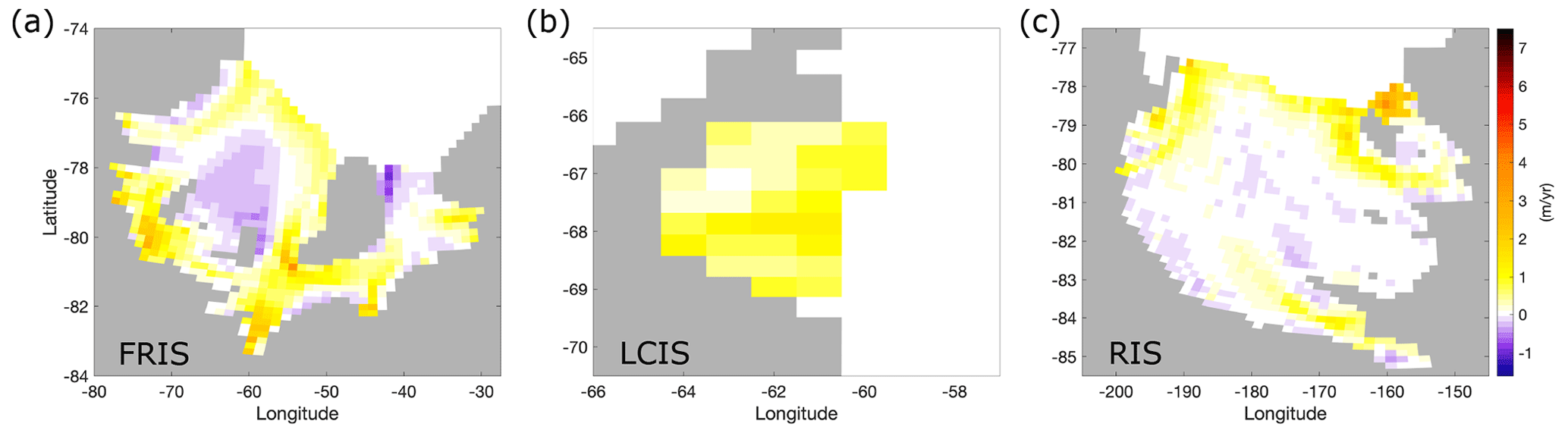
Figure 4 Melt rates in metres per year for (a) Filchner-Ronne Ice Shelf, (b) Larsen C Ice Shelf and (c) Ross Ice Shelf, where orange indicates melt and purple re-freezing. The results are mean values for the model equivalent period 1995–2009.

Table 1 Comparison of mean total melt flux (gigatonnes per year) for the Filchner-Ronne Ice Shelf (FRIS), Larsen C Ice Shelf (LCIS) and Ross Ice Shelf (RIS) for observational and model studies. The mean and standard deviation of all the estimates depicted in the table excluding the current study are shown at the bottom.

The patterns of melt shown in Fig. 4 also compare well with those of observational estimates like Rignot et al. (2013; their Fig. 1) and high-resolution model results like Hausmann et al. (2020; their Fig. 3), whose colour bar we replicated for ease of cross-comparison. If we look at the melt pattern of FRIS and compare it with these two aforementioned studies, we see that eORCA1 captures the high melt rates at the western portion of the ice shelf front, at the southern edge of Berkner Island and along the grounding line at the back of the cavity. The model also correctly simulates the region of refreezing along the western boundary of the circulation cell within the cavity, in both the Ronne and Filchner depressions and the re-freezing in the shallow region between the Korff and Henry Ice Rises (Fig. 4a, see bathymetry location in Fig. 1a). For LCIS, the entire shelf shows a positive melt (Fig. 4b). Observations from Rignot et al. (2013) and simulations from Harrison et al. (2022) indicate some re-freezing under this ice shelf, but the regional high-resolution model studies of Mathiot et al. (2017) and Hausmann et al. (2020) similarly show melting only. The pattern for RIS generally compares well with that reported from observations, but the magnitude of melt at the ice shelf front, especially to the east, is elevated (Fig. 4c).

4.2 Circulation and properties

Opening the sub-ice shelf cavities in eORCA1 allows for the establishment of a horizontal gyre circulation within the cavity and on the continental shelf of the Weddell Sea and the Ross Sea, in line with previous studies (Losch, 2008; Mathiot et al., 2017).

The mean state of circulation from the last 10 years of simulation within the FRIS cavity, along with the associated bottom thermohaline properties, can be seen in Fig. 5a–d. The circulation patterns shown here are in good agreement with Bull et al. (2021) at $\mathrm{1}/\mathrm{4}$^∘ and with Hausmann et al. (2020) at $\mathrm{1}/\mathrm{12}$^∘, with the exception of higher bottom salinities in eORCA1 and a slightly weaker barotropic circulation strength. Note that here we use potential temperature and practical salinity so as to be in line with the other figures of this paper, so approximately 0.17 psu must be added when juxtaposing with absolute salinity plots. The depth-averaged velocity and barotropic circulation pattern in Fig. 5a and b both indicate an anticlockwise circulation under the ice shelf. Comparatively warm and salty HSSW enters via the Ronne Depression, circulates from west to east, melts the base of the ice shelf mostly along the grounding line (cold, fresh signatures in Fig. 5c and d) and exits via the Filchner Trough as ISW. This pattern is consistent with observations (Nicholls et al., 2001; Janout et al., 2021). Two pathways of Modified Circumpolar Deep Water (MCDW) towards the ice shelf front can be seen, both in the circulation pattern (Fig. 5a) and via the bottom temperature (Fig. 5c): one located in the middle of the continental shelf (Central Trough) and the other on the shelf to the east of Filchner Trough. These pathways provide a conduit for heat towards the ice shelf and facilitate the mixing of shelf water masses with MCDW. It is therefore encouraging that eORCA1 (with an effective horizontal resolution under FRIS of 22 km) captures these, as they could play an important role in the evolution of shelf circulation in future climate scenarios (Naughten et al., 2021).

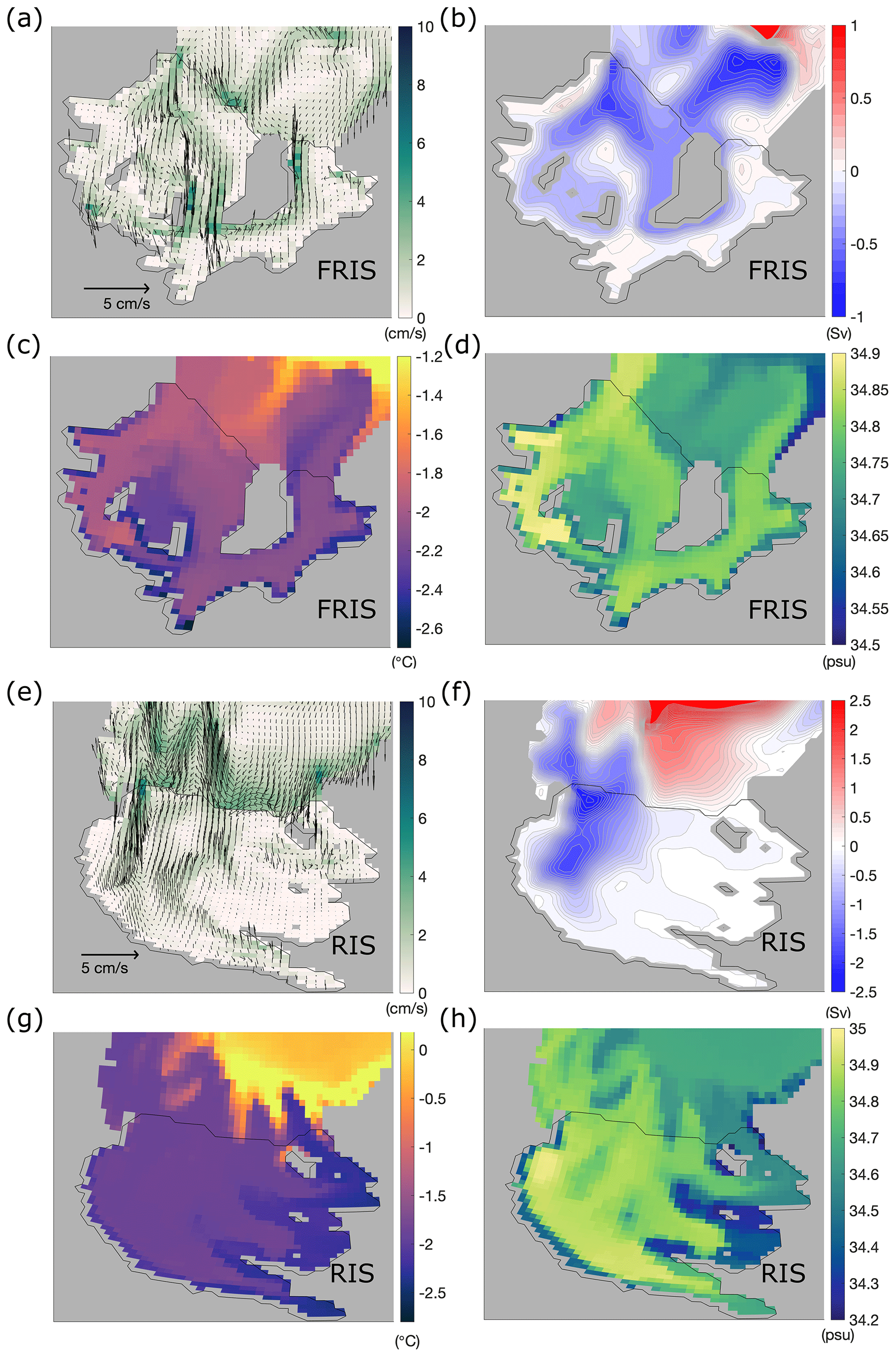
Figure 5 Circulation pattern and characteristics of properties under the Filchner-Ronne Ice Shelf (a–d) and the Ross Ice Shelf (e–h) for the last 10 years of the open-cavity experiment. Panels (a) and (e) show depth-averaged velocity, (b) and (f) barotropic stream function, (c, g) bottom potential temperature, and (d) and (h) bottom practical salinity (as opposed to conservative and absolute shown in Bull et al., 2021).

Moving now to the Ross Sea, the time mean circulation pattern under RIS along with the bottom temperature and salinity can be seen in Fig. 5e–h. Here, we notice a strong anticlockwise circulation concentrated at the western boundary, with reduced magnitude currents towards the back and east of the cavity. The west of the cavity is overall warmer and saltier and the east shows signatures of ISW. Bottom temperature indicates the presence of a cold ISW plume exiting the cavity to the far east (Fig. 5g), which is not seen in the time-averaged velocities or barotropic streamfunction, likely because the associated speeds are slow. Instead, the simulated circulation indicates an offshore advection of sub-ice shelf water following the Challenger Trough (see location marked in Fig. 1b). This water mass is likely recirculated HSSW as its temperature remains at surface freezing point (−1.9 ^∘C). A strong clockwise circulation cell offshore of RIS (red in Fig. 5f) brings warm CDW into contact with the ice shelf front to the east, mixing out the signature of ISW further offshore (Fig. 5g). While this simulated circulation pattern agrees well with that described by observations (Fig. 1; Bergamasco et al., 2003; Budillon et al., 2003), it is likely too strong, resulting in an exaggerated net melt flux compared to the observational estimates (Table 1; anomalously high melt at the eastern portion of the ice shelf front in Fig. 4c).

4.3 Impact on offshore properties

To highlight the impact of opening the FRIS, LCIS and RIS sub-ice shelf cavities on the offshore properties, Figs. 2g and 3g show the temperature versus salinity distribution excluding the data under the ice shelves. The differences in bottom temperature and salinity can be seen in Fig. 2h and i for the Weddell Sea and Fig. 3h and i for the Ross Sea.

A significant improvement in the representation of Weddell shelf water properties is evident as now HSSW is within the observed range and ISW is detected on the continental shelf (see HSSW and ISW red boxes in Fig. 2g). Opening the sub-ice-shelf cavity of FRIS has allowed the HSSW that previously built up in the Ronne Depression to advect under the ice shelf, become modified through basal interactions, and exit the cavity as colder and fresher ISW. Consequently, the temperature and salinity differences are polarized west and east, with warmer fresher conditions along the entire western boundary of the Weddell Gyre and cooler, saltier conditions on the eastern continental shelf (Fig. 2h and i). These results agree well with those of Mathiot et al. (2017). The impact of opening LCIS can be seen via the maintenance of cold bottom properties immediately to the north (despite the fact that the shelf circulation has changed so that HSSW no-longer floods this region), along with the presence of a large negative salinity anomaly indicative of ice shelf melt (Fig. 2i). As the simulation is only 124 years long, the impact of opening the cavities on AABW cannot be fully assessed due to the slow renewal of this water mass at the bottom of the global ocean. A small change in signature of AABW can, however, be seen in the volumetric T–S plot (Supplement Fig. S3a), where explicit ocean–ice shelf interaction results in a shift in volume towards cooler, fresher AABW (open−closed weighted average shift in AABW volume by −0.008 ^∘C and −0.003 psu). This shift is accompanied by a small increase in volume of the water mass by 0.23 % (AABW limits delineated in green in Fig. S3a).

The impact of opening the RIS cavity on offshore properties can be seen in Fig. 3h and i. Similar to the Weddell Sea, conditions in the west, where in the reference run HSSW was built up, now become warmer and fresher as the path under the ice shelf is open. The signature of the cold plumes of dense shelf water (Fig. 5g) on either side of Roosevelt Island can clearly be seen in the temperature difference plot (Fig. 3h), but curiously they do not possess the same salinity anomaly (Fig. 3i). The positive salinity difference of the western plume indicates that this water is a variety of HSSW which has circulated under the ice shelf and was previously not present in this area. The small negative anomaly to the east indicates that this cold plume is, as previously hypothesized, outflowing ISW. Small temperature differences on the continental slope and further offshore indicate that there has been some communication of the changes in shelf waters further afield. The volumetric T–S plot for the Ross Sea found in the Supplement (Fig. S3b) indicates that opening the RIS cavity has moved the core of AABW towards slightly cooler fresher values, accompanied by a 0.34 % decrease in volume of AABW as defined by the original water mass limits (delineated in green in Fig. S3b; open−closed weighted average shift in AABW volume by −0.001 ^∘C and −0.005 psu).

4.4 Comparison with ice shelf front CTD observations

The differences in circulation patterns and in thermohaline properties that result from opening the RIS and FRIS cavities documented above do not elucidate whether or not we have reduced biases and improved the realism of shelf waters in eORCA1. For this, a direct comparison with in situ observations is necessary. Due to the remote location of these ice shelves and the harsh conditions associated with obtaining hydrographic samples in these areas, there are limited observations, and so optimally interpolated atlases such as WOA or ocean reanalysis products like SOSE miss important local features or seasonal variability. For comparison purposes, we have consequently selected CTD data from research cruises that have sampled transects across the front of the ice shelves and extracted the model data corresponding to the approximate ship's track using PAGO, a tool to analyse gridded ocean datasets (Deshayes et al., 2014).

For FRIS we use two CTD sections across the ice shelf front undertaken in 1980 and 1995 on board the RV Polarstern by the Alfred Wegener Institute (Rohardt et al., 2016; Janout et al., 2021). The location of the section selected in NEMO to approximately overlay the CTD transects can be seen as a dotted magenta line in Fig. 1a. The output from NEMO corresponding to the same months and same equivalent year (for the second cycle of CORE forcing) in the simulation was selected for both closed-cavity (prescribed freshwater flux) and open-cavity (FRIS, LCIS and RIS) runs. A comparison between the CTD data and NEMO can be seen in Fig. 6a to f for January 1980 and Fig. 6g to l for February to March 1995. In terms of surface waters, NEMO does not capture the fine-scale horizontal variability and overestimates the subsurface salinity. For both observational years, evidence of warm, fresh, MCDW intrusions can be seen in the middle of the CTD sections (Central Trough; Fig. 6a and g). While the model struggles to capture the coherence of this subsurface temperature maximum, the anticlockwise circulation cell set up on the central continental shelf in the open-cavity simulation does aid the advection of MCDW towards the ice shelf, thereby producing a slightly better representation of this warm intrusion in Fig. 6c and i. The presence of cold ISW in Filchner Trough is clearer in the 1995 CTD data than in 1980, where the sampling frequency was sparser and this region not well covered. The 2018 Polarstern sampling of the Jason Trough was the highest resolution yet, and while we cannot directly compare with the simulation output as the CORE forcing ends in 2009, the presence of a tongue of ISW focused on the western bank of Filchner Trough is evident in Fig. 3 of Janout et al. (2021) and so should be kept in mind for comparison. Opening the FRIS cavity overall improves the thermohaline properties at the ice shelf front, most notably by spreading out the pool of HSSW from the Ronne Depression (e.g. Fig. 6k) across the continental shelf (e.g. Fig. 6l) and by facilitating the production and thus outflow of ISW within Filchner Trough (Fig. 6c and i).

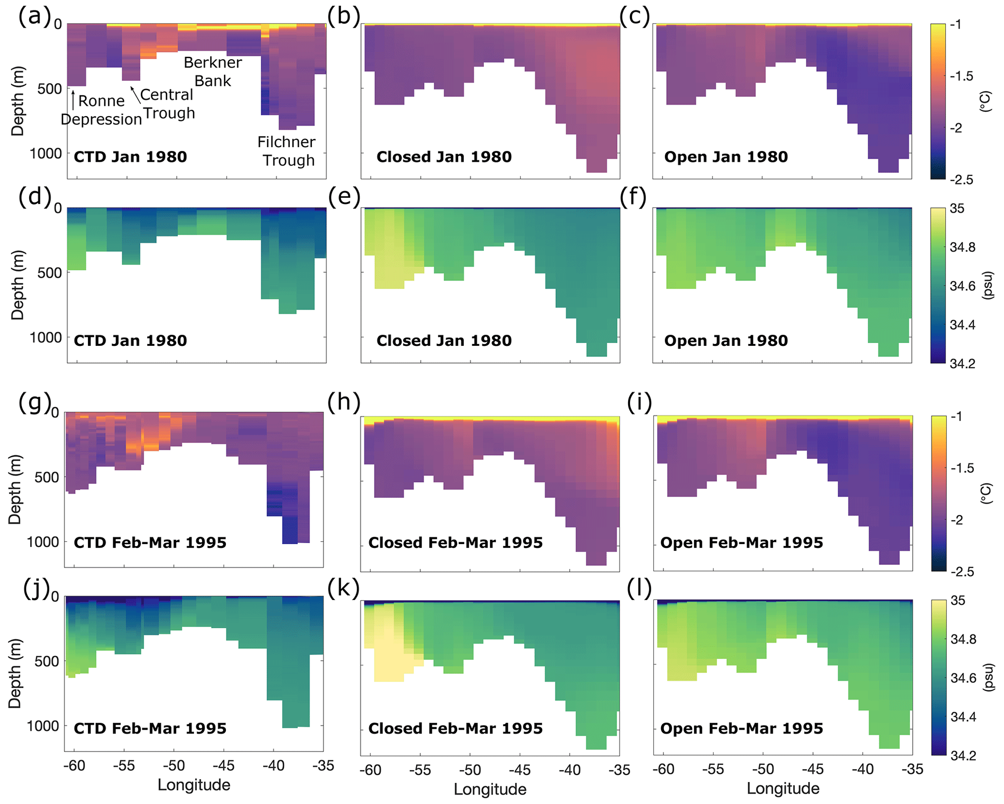
Figure 6 Validation of properties across the Filchner-Ronne Ice Shelf front by comparing closed- and open-cavity NEMO results with measured values from CTD sections performed in 1980 (Rohardt et al., 2016) and 1995 (Janout et al., 2021). The model output for the corresponding equivalent year and month was extracted for more accurate comparison. Bathymetric features discussed in the text are labelled in (a).

The CTD sections used for comparison along the front of RIS were obtained through the World Ocean Circulation Experiment Database (Boyer et al., 2018) and correspond to cruises undertaken on board the RVIB Nathaniel B. Palmer in 2000 (cruise id: US010404; Smethie and Jacobs, 2005) and in 2007 (cruise id: US034357). Data were extracted from the eORCA1 simulation corresponding to the dates of these cruises and the approximate ship track across the ice shelf front (dotted magenta line in Fig. 1b). Similar to the Weddell Sea, the model tends to overestimate the subsurface temperature and salinity (Fig. 7b, e, h and k), suggestive of biases in the representation of coastal processes, including vertical mixing. This effect is somewhat reduced by allowing for circulation under RIS, especially by decreasing subsurface salinities (Fig. 7f and l). At depth, NEMO captures the east–west distribution of haline properties such as the HSSW pool located within Joides Basin, albeit with somewhat amplified salinities. In terms of temperature, the model has a clear bias to the east, especially in the closed-cavity run, where CDW is detected at the ice shelf front. Both the temperature and salinity biases are reduced in the open-cavity run (e.g. Fig. 7c and f). In particular, the significant reduction in the extent and magnitude of the subsurface warm water intrusions brings the model more in line with observations.

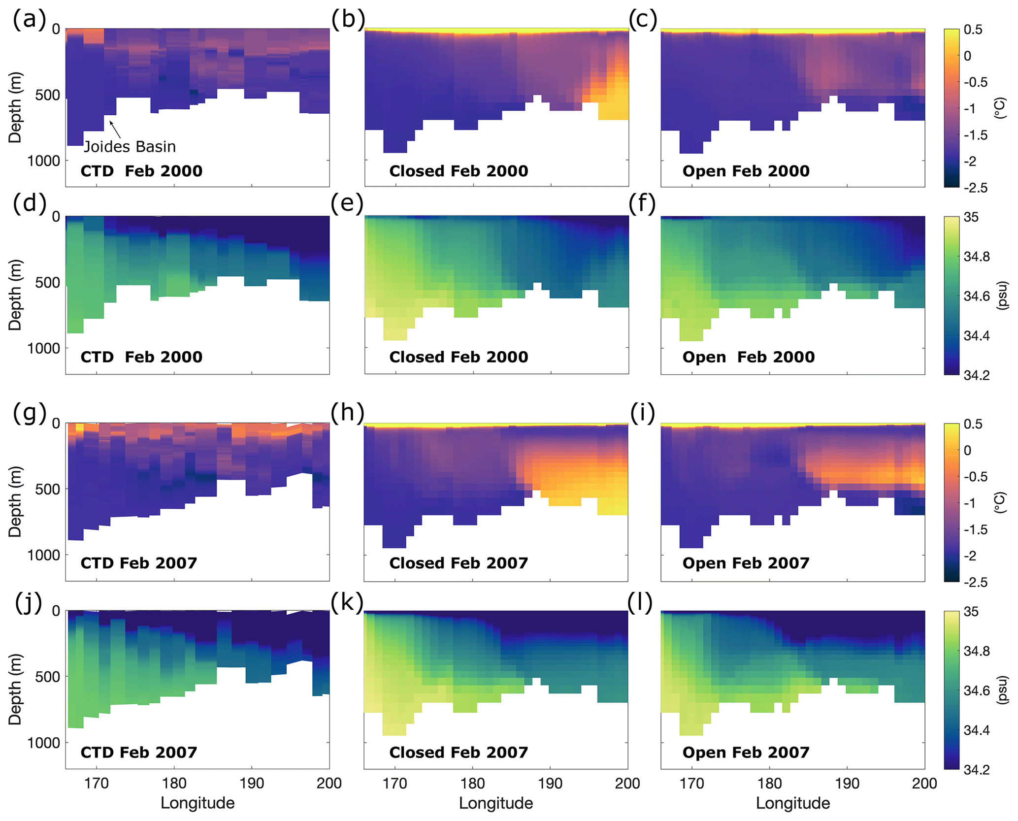
Figure 7 Same as Fig. 7 but for Ross Ice Shelf front for CTD sections performed in 2000 (Smethie and Jacobs, 2005) and 2007 (Boyer et al., 2018).

A recurring theme throughout the results presented here is that the model is overall too salty, driven by what appears to be an over-production of HSSW in the Ronne Depression and Joides Basin. One driver for this could be the overestimated polynya activity which forms the totality of parent waters of AABW in the absence of ice shelves in eORCA1. This can be seen in Fig. 8 where the mean winter (July–August–September) mixed-layer depths (MLDs) in the reference run for the years 1971–2009 are compared to the climatology from Sallée et al. (2021a) for the same time period and using the same criteria for calculation (Fig. 8a and b; MLD defined as the depth at which density exceeds the 10 m density by 0.03 kg m⁻³). The model greatly overestimates winter MLDs in the Weddell Sea, both on the continental shelf adjacent to FRIS, where the depth of the base of the mixed layer aligns with bathymetric features indicating deep convection right to the ocean floor, and offshore of the continental slope, where a large region of MLD greater than 1000 m is present (Fig. 8c). This level of open-ocean deep convection has in reality only once been observed, during the 1974–1976 Weddell Polynya event near Maud Rise (3^∘ E, 66^∘ S), indicating a gross overestimation of winter MLDs in the model (Heuzé, 2021; Killworth, 1983). Ross Sea MLDs (Fig. 8d) compare better with observations but show values indicating a full water-column-depth convection in Terra Nova Bay which is not reported in Sallée at al. (2021a). Curiously, NEMO actually underestimates winter mixed layers in the eastern portion of the Ross continental shelf showing mean MLDs of under 100 m where the observational climatology indicates values of around 400 m (Fig. 8d compared to Fig. 8b). This too strong a stratification could be one of the factors facilitating the intrusion of CDW to the ice shelf front seen in Fig. 7b and h.

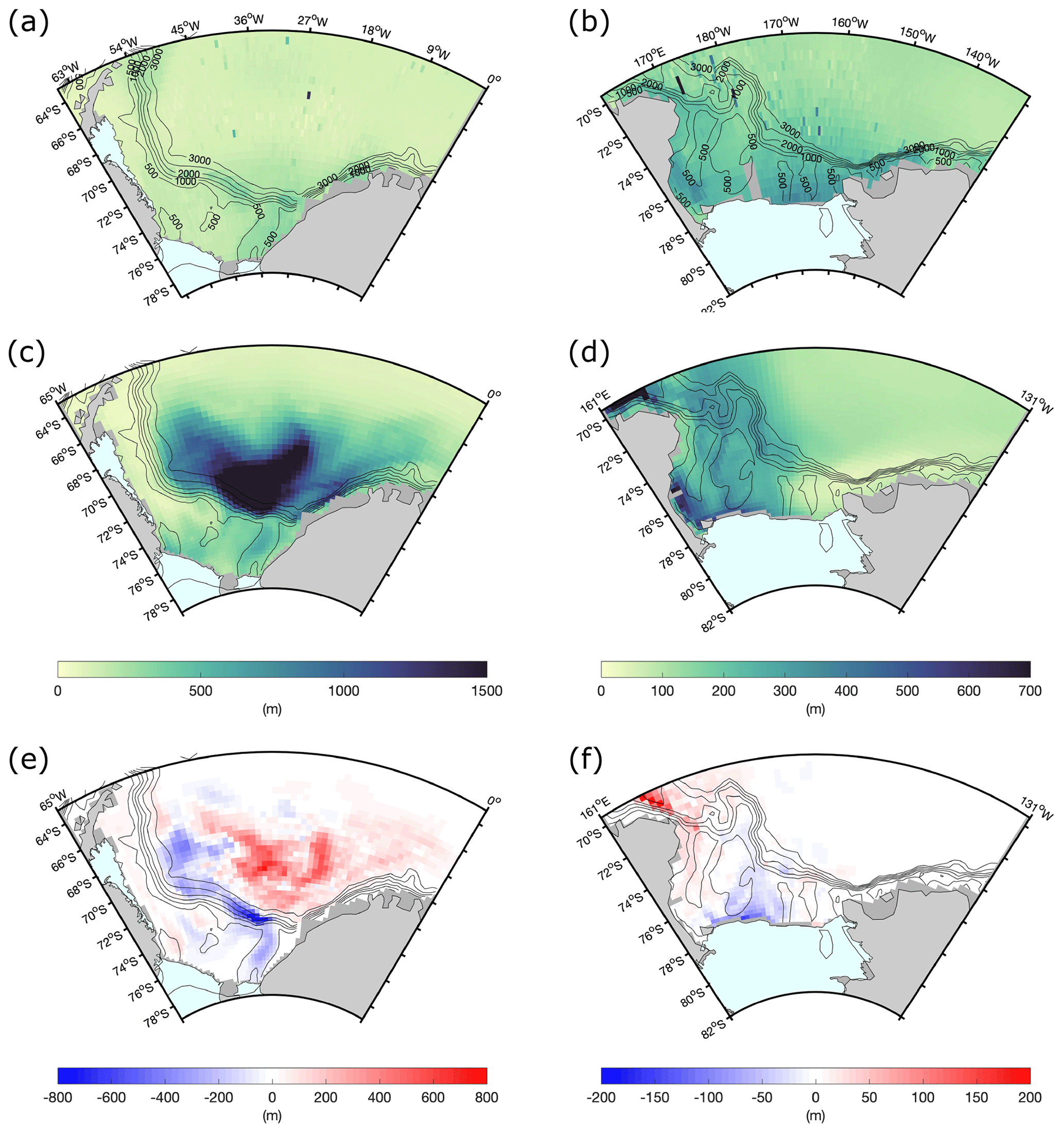
Figure 8 Winter mixed-layer depths (MLDs) from the observational atlas of Sallée et al. (2021a), shown in (a) and (b) for the Weddell Sea and the Ross Sea respectively, are compared with the winter mean from NEMO v4.2 eORCA1-forced model reference configuration equivalent years 1971–2009 in (c) and (d). The differences in MLDs between the open-cavity run and reference closed run are shown in (e) and (f).

The authors note that the biased MLDs could be one of a number of factors contributing to the overly saline conditions; wrong sea ice parameters and biases in the atmospheric forcing could also play an important (and related) role. High sea ice production is seen on the southwest continental shelves of the Weddell Sea and Ross Sea in the Supplement Fig. S2a and b. Opening the cavities slightly reduces the magnitude of ice production in the Ronne Depression (Fig. S2c) and at the location of the Terra Nova Bay polynya (Fig. S2d) and increases the production of ice further east. There is no overall change in the principal location of polynya activity, and the slight west/east decrease/increase in sea ice is presumed to have a negligible effect on the total amount of HSSW generated. As such, the reduction of the highly saline HSSW signature seen in Figs. 2g and 3g when cavities are opened is likely due to a conversion to ISW (and not from a decrease in HSSW production itself). Please see the Supplement Sect. S3 for an evaluation of simulated polynyas near the studied ice shelves and a diagnosis of the effect of opening the cavities on ice production.

Once a model is able to explicitly form the parent waters of AABW in the right locations on the continental shelf (and export this dense water), it will become necessary for modellers to tone down open-ocean deep convection as this workaround will be longer relied upon to form the totality of AABW. Here we explore the impact that opening the cavities has on MLD to diagnose the extent of vertical convection in the model. Some reduction in MLD is seen on the continental shelf and slope in the Filchner (Fig. 8e) and Challenger troughs (Fig. 8f) due to the increase in stratification as a result of the greater bottom densities associated with outflowing ISW (Fig. S4a and c). The presence of ISW appears to promote slightly increased ice production in these areas, as discussed earlier. In this case, it is therefore the ocean properties that drive sea ice, and the brine rejection associated with elevated ice production is found to have a minor effect on water properties. Within the region of exaggerated MLDs off the Weddell continental slope, the MLDs deepen in the open-cavity experiment (positive anomalies Fig. 8e). We hypothesize that this deepening is associated with an overall cooling of the subsurface layers due to a horizontal mixing of ISW, unimpeded by a relatively weak and diffuse Antarctic Slope Current (ASC; discussed in the following section). Overall, in wintertime, mixed layers are on average 19 m deeper over the whole Weddell Sea region in the open-cavity experiment compared to the reference closed simulation. This reinforcement of the high MLD bias highlights the need for work to be done on reducing wintertime deep convection, together with better representing dense water overflows.

4.5 Offshore export of continental shelf properties

We have seen how opening the large, cold ice shelf cavities in eORCA1 leads to a better representation of continental shelf circulation and thermohaline property distributions. But the question remains regarding the transfer of these now more realistic dense shelf waters downslope and offshore, to feed the globally important AABW. While the simulation period of 124 years (two CORE forcing cycles) is too short to explore the impact of these changes far afield, it is sufficient to investigate the changes on the continental shelf and slope adjacent to the large ice shelves. To do this, we use PAGO (Deshayes et al., 2014) to select a cross section of data following the bathymetric troughs of the Weddell Sea and the Ross Sea, which are thought to be important for dense water export (Foldvik et al., 1985; Jacobs, 1991), namely the Filchner and Challenger troughs (sections shown in green in Fig. 1).

The thermohaline cross sections of Filchner Trough and a continuation down the continental slope can be seen in Fig. 9a and b for the open-cavity run, and the difference between these values and the reference run (open−closed) is shown in Fig. 9c and d. By opening the sub-ice shelf cavity, the properties within Filchner Trough have decreased in temperature and increased in salinity as the candidate parent waters of AABW build up on the continental shelf. This results in a net increase in density at the bottom of the trough (Fig. S4b), but there is very little indication of a coherent cascading of this water down the continental slope.

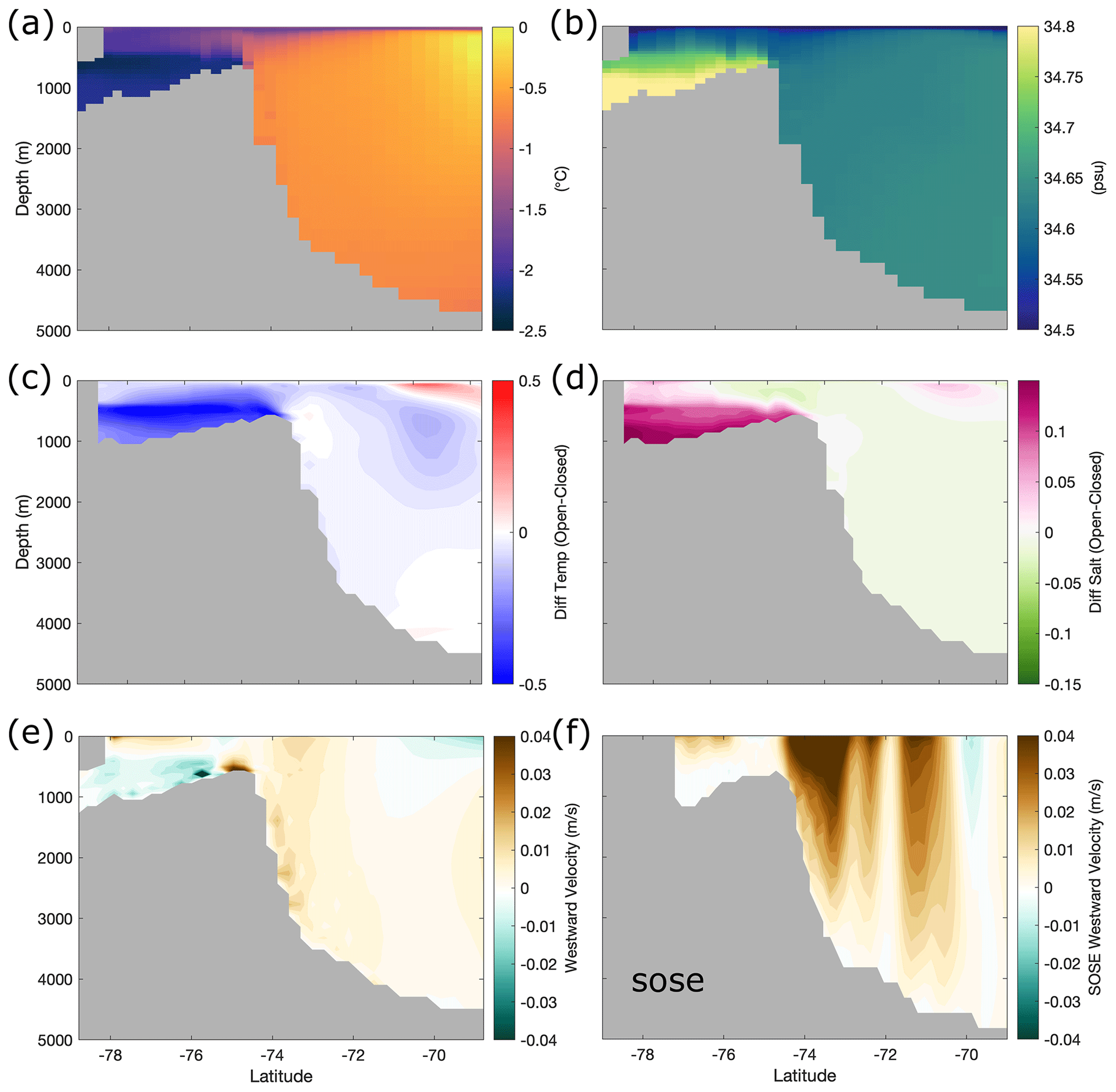
Figure 9 Cross section of properties along the Filchner Trough and down the adjacent continental slope of the Weddell Sea for (a–e) NEMO and (f) SOSE. Panels (a) and (b) show temperature and salinity for the open-cavity configuration, to be compared to (c) and (d) which show the differences (open−closed) with the reference configuration. Panel (e) shows cross-sectional velocities with westward as positive for the open-cavity run, to be compared with SOSE values shown in (f).

A cross section of the Challenger Trough (Fig. 10) reveals depth-varying thermohaline changes. Opening the sub-ice shelf cavity has allowed for the water adjacent to the ice shelf to advect into the cavity leaving the bottom properties here slightly warmer. The layer immediately above conversely experiences cooling and salinification due to the outflow of ISW driven by the “ice pump” (Fig. 10c). Here we see some evidence indicating the translation of this dense cold water tongue over the continental shelf break and downslope (Figs. 10c and S4d). The overflow of this water results in the pulling in of warmer offshore water at intermediate depth (Fig. 10c). A horizontal redistribution of surface waters simultaneously takes place due to the anti-clockwise circulation pattern (Fig. 5e), which in turn produces a cooling and freshening in the surface layer (Fig. 10c and d).

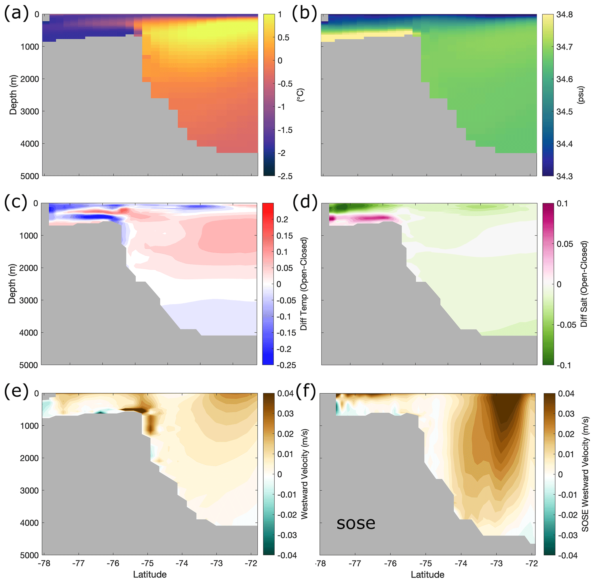
Figure 10 Same as Fig. 9 but for the Challenger Trough and the Ross Sea continental slope.

For both the Filchner and Challenger troughs, the downslope export of the ISW tongue is limited due to the commonly known and acknowledged problem of correctly capturing this overflow in a coarse z-coordinate model (Heuzé, 2021). The aptitude of representing dense water overflows is thought to increase with models of higher resolution, but this is difficult to achieve in a global model for climate coupling purposes without a nested zoom (Storkey et al., 2018; Colombo et al., 2020; Solodoch et al., 2022).

Another important dynamic for Antarctic shelf water realism is the ASC (red arrows in Fig. 1) and related Antarctic Slope Front, which together restrict the lateral mixing of offshore and shelf water masses, acting as an effective barrier protecting the large, cold ice shelves from warm water masses of circumpolar origin (Thompson et al., 2018). Some CDW, or a modified version thereof, is carried within the ASC and occasionally fluxes onshore to mix with dense shelf waters (Beadling et al., 2020; Bull et al., 2021). This interaction between dense shelf water and CDW is important for the formation of AABW, as the onshore flux of water replaces the dense water transported offshore and thus sustains formation of shelf water (Thompson et al., 2018). Figure 9e shows a velocity cross section for the Weddell Sea shelf and slope where westward velocities are positive so as to correspond with the direction of the ASC, and the net westward transport across the section is 9.8 Sv (1 Sv is 10⁶ m³ s⁻¹). This can be compared to Fig. 9f, which is a cross section from SOSE output (same time periods used) where the net transport is 3 times higher at 32.8 Sv. Similarly for the Ross Sea, Fig. 10e shows a cross section of westward velocities in eORCA1 where the volume transport is 13.3 Sv, which is less than half of that estimated from SOSE in Fig. 10f of 20.9 Sv. As can be seen from both SOSE cross sections, the ASC flows eastward as a narrow jet, closely following the shelf break in the Weddell Sea and slightly further offshore in the Ross Sea. It is well known that coarse-resolution models are unable to correctly represent the ASC as a resolution of at least 0.5^∘ is needed to capture the dynamics and net transport (Mathiot et al., 2011). The absence of realistic ASC in NEMO eORCA1 (Figs. 9e and 10e) has important consequences, as a weaker and more diffuse ASC allows for a greater level of onshore–offshore exchange of water masses. This is one important restriction that needs to be kept in mind when using this coarse-resolution configuration for process studies in the area.

5 Summary and discussion

Explicitly representing ocean–ice shelf interactions is of great interest to modellers as these processes play an important role in global ocean dynamics, climate and future sea level rise. The formation of dense shelf waters (HSSW and ISW) along the Antarctic coastline provides the principal source for AABW, which in turn facilitates the ventilation of the deep ocean and constitutes the lower limb of the global overturning circulation (Killworth, 1983; Johnson, 2008; Orsi, 2010).

Our results focus on the Weddell Sea and the Ross Sea as they are respectively the main ventilation source of the abyssal Atlantic and Indian basins and the abyssal Pacific basin (Solodoch et al., 2022). Explicitly simulating the sub-ice shelf cavities of FRIS and LCIS in the Weddell Sea leads to a re-organization of continental shelf circulation with thermohaline patterns in agreement with those reported by other NEMO model studies (Mathiot et al., 2017; Storkey et al., 2018 and Bull et al., 2021), namely warming and freshening in the west and cooling and salinification in the east. Notably, opening a pathway for HSSW under FRIS allows for an anticlockwise circulation of water under the ice shelf, triggering basal melt and re-freezing and producing the super-cold ISW.

By comparing model output with two CTD sections performed across the front of FRIS in 1980 and 1995 (Rohardt et al., 2016; Janout et al., 2021), we see clear evidence of an improvement in the realism of water properties with the opening of the sub-ice shelf cavity. Similarly in the Ross Sea, an anticlockwise sub-ice shelf cavity circulation cell facilitates the spread of HSSW across the continental shelf, and ocean–ice shelf interactions create a cold ISW plume to the east of Roosevelt Island. By evaluating the model output against CTD sections performed in 2000 and 2007 (Smethie and Jacobs, 2005; Boyer et al., 2018), we see that opening the cavity significantly ameliorates the subsurface warm water bias otherwise seen to the east of RIS in the reference configuration and brings a significant improvement in the horizontal thermohaline distributions.

The mean total melt fluxes of FRIS, LCIS and RIS are found to be within the uncertainty range of observational estimates and other model studies. Notably, the melt rate pattern of FRIS agrees surprisingly well with the high-resolution regional model of Hausmann et al. (2020) and the satellite observations of Rignot et al. (2013), showing details of melt and refreezing that were not expected at a 1^∘ resolution, although the meanders of the grounding line are not well represented at 1^∘. For RIS, the net melt is higher than all observed estimates but lower than that predicted by other model studies. RIS melt rates are strongly related to the supply of warm water to the ice shelf base (Arzeno et al., 2014), and correctly representing this in models presents a challenge due to the close proximity of CDW to the ice shelf front in this area.

Meltwater and modified HSSW mix on the continental shelves of the Weddell Sea and Ross Sea and in reality cascade down the continental slope, mixing with ambient water masses during the descent, to eventually feed AABW. This process is poorly represented in NEMO eORCA1, a common problem with coarse z-coordinate models, as exaggerated vertical and horizontal mixing erodes the signatures of the dense overflow tongue. As mentioned by Storkey et al. (2018), the use of a terrain following coordinate system (known as sigma coordinate) can greatly improve the representation of these density currents and so is something worth exploring in the future. Improvement in the representation of the overflows along with a reduction of open-ocean deep convection should together allow for a coherent communication of the now more realistic properties of dense water on the continental shelf offshore to AABW.

6 Conclusions

In this paper the authors focus on improving the properties of AABW parent waters in a global NEMO configuration. We compare the model simulations with in situ observations, in addition to gridded climatologies, so as to deepen understanding and expertise regarding the impact of opening sub-ice shelf cavities on ocean dynamics. As ocean models used for climate simulations with multiple scenarios (such as CMIP) need to be at a coarse resolution to permit long integrations, we use the NEMO global ocean 1^∘ configuration, eORCA1, here. The results presented are for CORE inter-annual forcing, with a fixed cavity geometry, as this allows us to clearly identify the impact of ocean–ice shelf interactions at a few critical locations without the obscuring effect of coupling feedbacks. We present here a validated configuration of NEMO 4.2 eORCA1 with explicit ocean–ice shelf interactions only within the largest three cold cavities: FRIS, LCIS and RIS. Limitations of this choice are that together FRIS, LCIS and RIS only represent 63 % of the total area of Antarctic ice shelves, and, while they are responsible for the formation of the majority of the parent waters of AABW, interactions with remote unresolved ice shelves are missing (Nakayama et al., 2020). The next steps in terms of increasing complexity in NEMO eORCA1 are to open other intermediate size cavities, such as Amery, Riiser-Larsen and Fimbul, in a fixed geometry configuration, and leave smaller cavities parameterized due to resolution constraints. As the residence time needed to flush these intermediate cavities is shorter than for FRIS and RIS, we suggest that the complex initialization methods presented here are not needed. This work is aimed at building understanding so as to eventually move to coupling with an ice sheet model, thereby allowing for fully evolving cavity geometry and iceberg calving from the ice shelf front.

Given the critical role that the Southern Ocean plays in regulating global climate, it is paramount that ocean models work towards improving the representation of key processes in order to provide state-of-the-art simulations of the ocean in a changing climate (Beadling et al., 2020). The global configuration of NEMO presented here has been proven to improve the realism of water masses in the Weddell Sea and the Ross Sea. We advocate for climate modellers to use it, as it enables a more accurate representation of the formation of the parent waters of AABW, and it is a first step in the perspective of representing ocean–ice shelf interactions in climate applications.