the Creative Commons Attribution 4.0 License.
the Creative Commons Attribution 4.0 License.
 | 13 Jun 2023
Predicting the climate impact of aviation for en-route emissions: the algorithmic climate change function submodel ACCF 1.0 of EMAC 2.53
Volker Grewe
Federica Castino
Pratik Rao
Sigrun Matthes
Katrin Dahlmann
Simone Dietmüller
Christine Frömming
Hiroshi Yamashita
Patrick Peter
Emma Klingaman
Keith P. Shine
Benjamin Lührs
Florian Linke
Using climate-optimized flight trajectories is one essential measure to reduce aviation's climate impact. Detailed knowledge of temporal and spatial climate sensitivity for aviation emissions in the atmosphere is required to realize such a climate mitigation measure. The algorithmic Climate Change Functions (aCCFs) represent the basis for such purposes. This paper presents the first version of the Algorithmic Climate Change Function submodel (ACCF 1.0) within the European Centre HAMburg general circulation model (ECHAM) and Modular Earth Submodel System (MESSy) Atmospheric Chemistry (EMAC) model framework. In the ACCF 1.0, we implement a set of aCCFs (version 1.0) to estimate the average temperature response over 20 years (ATR20) resulting from aviation CO2 emissions and non-CO2 impacts, such as NOx emissions (via ozone production and methane destruction), water vapour emissions, and contrail cirrus. While the aCCF concept has been introduced in previous research, here, we publish a consistent set of aCCF formulas in terms of fuel scenario, metric, and efficacy for the first time. In particular, this paper elaborates on contrail aCCF development, which has not been published before. ACCF 1.0 uses the simulated atmospheric conditions at the emission location as input to calculate the ATR20 per unit of fuel burned, per NOx emitted, or per flown kilometre.
In this research, we perform quality checks of the ACCF 1.0 outputs in two aspects. Firstly, we compare climatological values calculated by ACCF 1.0 to previous studies. The comparison confirms that in the Northern Hemisphere between 150–300 hPa altitude (flight corridor), the vertical and latitudinal structure of NOx-induced ozone and H2O effects are well represented by the ACCF model output. The NOx-induced methane effects increase towards lower altitudes and higher latitudes, which behaves differently from the existing literature. For contrail cirrus, the climatological pattern of the ACCF model output corresponds with the literature, except that contrail-cirrus aCCF generates values at low altitudes near polar regions, which is caused by the conditions set up for contrail formation. Secondly, we evaluate the reduction of NOx-induced ozone effects through trajectory optimization, employing the tagging chemistry approach (contribution approach to tag species according to their emission categories and to inherit these tags to other species during the subsequent chemical reactions). The simulation results show that climate-optimized trajectories reduce the radiative forcing contribution from aviation NOx-induced ozone compared to cost-optimized trajectories. Finally, we couple the ACCF 1.0 to the air traffic simulation submodel AirTraf version 2.0 and demonstrate the variability of the flight trajectories when the efficacy of individual effects is considered. Based on the 1 d simulation results of a subset of European flights, the total ATR20 of the climate-optimized flights is significantly lower (roughly 50 % less) than that of the cost-optimized flights, with the most considerable contribution from contrail cirrus. The CO2 contribution observed in this study is low compared with the non-CO2 effects, which requires further diagnosis.
- Article
(6194 KB) - Full-text XML
-
Supplement
(1763 KB) - BibTeX
- EndNote


Civil aviation satisfies modern society's mobility needs and is an essential economic driver. Air transportation demand increases at around 4.4 % yr−1 and is forecast to maintain that growth for the next decades (Airbus, 2018). Though the global COVID-19 pandemic has put a tremendous challenge on the aviation industry, aviation (as a fundamental part of the modern world) will recover eventually. An example from the recent ICAO post-COVID forecast shows that the revenue passenger kilometres (RPK) is expected to grow at an annual average rate of 3.6 % with a low and high range between 2.9 % and 4.2 % over the next 3 decades from 2018 to 2050 (https://www.icao.int/sustainability/Pages/Post-Covid-Forecasts-Scenarios.aspx, last access: 17 May 2023).
On the other hand, the environmental impact of aviation is increasing at an evenly rapid pace. Aviation contributes 2.5 % to global anthropogenic CO2 emissions and is responsible for about 3.5 % of global warming (Lee et al., 2021). This is because the non-CO2 effects from aviation in the uppermost troposphere and lowermost stratosphere are as harmful to global climate change as CO2 emissions (Lund et al., 2017). The non-CO2 effects include ozone (O3) formation and methane (CH4) depletion (causing the primary mode ozone (PMO) and stratospheric water vapour (SWV) decrease) due to aviation NOx emissions (Stevenson et al., 2004; Köhler et al., 2013; Myhre et al., 2007; Szopa et al., 2021; Terrenoire et al., 2022), contrail cirrus (Heymsfield et al., 2010; Burkhardt and Kärcher, 2011; Schumann and Graf, 2013; Kärcher, 2018) and their alterations by aerosols direct and indirect effects (Kärcher et al., 2007; Penner et al., 2009; Myhre et al., 2013; Chen and Gettelman 2016), and the water vapour (H2O) effect (Wilcox et al., 2012). Some recent studies investigated how COVID-19 affects aviation's climate impact per NOx or contrails concerned. For instance, Voigt et al. (2022) conducted a measurement campaign to investigate atmospheric concentration changes. The authors observed a significant reduction in NOx at cruise altitudes, contrail coverage, and the resulting radiative forcing. Furthermore, Gettelman et al. (2021) show that the effect of COVID-19 reductions in flights reduces contrail formation, which is aligned with the other study. However, due to spatial and seasonal variability of contrail radiative forcing, the annual-mean contrail effective radiative forcing shows no significant changes. Since aviation is expected to recover, it is still essential to address various climate effects of aviation with regard to their mitigation. The non-CO2 effects depend not only on the emission quantity but also on the altitude, geographical location, time, and local weather conditions (e.g. Frömming et al., 2021). Therefore, it is possible to mitigate aviation's climate impact via operational measures to avoid climate-sensitive regions associated with non-CO2 effects (Grewe et al., 2017b; Sridhar et al., 2011; Yin et al., 2018; Matthes et al., 2020).
Information on the climate-sensitive regions, i.e. areas where the non-CO2 effects are significantly enhanced or reduced, is required to facilitate climate-optimized flight operations. In the earlier research within the EU-project REACT4C (http://www.react4c.eu, last access: 17 May 2023), Climate Change Functions (CCFs) were developed and implemented for flight trajectory optimization. The CCFs are 5D datasets (including longitude, latitude, altitude, time, and emission type) that describe the specific climate impacts, i.e. the average temperature change in kelvin per flown kilometre or per emitted mass of the relevant species (NOx and H2O) locally. The high-fidelity CCFs were computed for eight representative weather situations (five winter patterns and three summer patterns classified by Irvine et al., 2013) for the North Atlantic region (Frömming et al., 2021). Grewe et al. (2014a) discussed the development and verification procedure of CCFs thoroughly. Various application studies have demonstrated the effectiveness of the CCFs in climate-optimized trajectory calculations (Grewe et al., 2014b, 2017b). These studies show promising mitigation potential when using CCFs as inputs for flight trajectory optimization (e.g. a 10 % reduction in climate impact for a 1 % cost increase). One of the underlying challenges is that calculating these CCFs is computationally expensive. Thus, with the present computing performance, it is impossible to use CCFs for real-time calculation, which is necessary for future climate-optimized flight planning.
To this end, previous research initiated development (Irvine, 2017; Matthes et al., 2017; van Manen and Grewe, 2019) and tests (Rao et al., 2022) of the so-called algorithmic Climate Change Functions (aCCFs). The aCCFs are algorithmic approximations of the high-fidelity CCFs to represent the correlation of meteorological parameters (e.g. temperature and geopotential) at the time of emission and the respective average temperature response over a time horizon of 20 years (ATR20). Since the aCCFs are essentially mathematical approximations, they can be quickly implemented in numerical weather prediction (NWP) models, thereby serving as a means of advanced meteorological information for flight trajectory planning.
The ACCF submodel version 1.0 (ACCF 1.0) of the European Centre HAMburg general circulation model (ECHAM) and Modular Earth Submodel System (MESSy) Atmospheric Chemistry (EMAC) model is based on the aCCFs version 1.0 (aCCFs 1.0). The ACCF 1.0 calculates the ATR20 from individual emissions and the contrail cirrus effect as a function of the online calculated local weather parameters in EMAC. One can use the ACCF 1.0 in two different ways: (1) to study the sensitivity of non-CO2 effects (i.e. NOx, H2O, contrail cirrus) to weather parameters and (2) to couple it with a flight planning tool (e.g. EMAC/AirTraf; Yamashita et al., 2016, 2020) for climate-based route optimization.
This paper elaborates on the modelling approach, the characteristics, and the application of ACCF 1.0. Please note that, for the first time, we show a consistent set of aCCF formulas in terms of fuel scenario, metric, and efficacy (aCCFs 1.0). Due to the continuous development of aCCFs, we expect different versions of aCCFs to be released in the future. Accordingly, the ACCF submodel will be updated.
The structure of the paper follows that Sect. 2 provides a roadmap of the ACCF 1.0 development focusing on different considerations when deriving the first version of contrail aCCFs and the NOx and H2O aCCFs. Section 3 presents an overview of ACCF 1.0, including the model components and the individual aCCF formulas. The original correlations of the NOx and H2O aCCFs were derived in van Manen and Grewe (2019), whereas some coefficients in the equations are updated here for consistency. Furthermore, the contrail cirrus effect is explained in detail here (and in the Supplement). In Sect. 4, we evaluate the performance of the ACCF 1.0 outputs via two types of simulations. First, we compare the climatological aCCFs to other literature studies in terms of their latitudinal and vertical variability. Second, we use the tagging chemistry approach (contribution approach, Grewe et al., 2010, 2017a) to evaluate the reduction of NOx-induced O3 effect through climate-optimized flight trajectories based on the O3 aCCF formula. Section 5 implements the ACCF 1.0 with the complete sets of aCCFs in the AirTraf 2.0 to demonstrate the usage of ACCF 1.0 for climate-optimized flight trajectories. It has to be noted that the two demonstration exercises are academic case studies, which do not intend to suggest an efficient implementation of such climate-optimized trajectories as we present here the extreme case of only considering ecological effects while completely ignoring economic effects in the optimization (equivalent to a non-combined objective function). One could consider combining the cost and climate objectives in trajectory optimizations to identify eco-efficient flights (e.g. Matthes et al., 2023). Section 6 discusses further developments of aCCFs before concluding in Sect. 7.
The new MESSy submodel ACCF 1.0 consists of a set of aCCFs 1.0, which take relevant local meteorological data as inputs to calculate the ATR20 for a given emission or effect concerning contrails. As introduced above, the roadmap toward the ACCF 1.0 model involves multiple stages of work originating from different research projects. Figure 1 illustrates the development of the ACCF 1.0, including the previous research on the original CCFs development followed by the aCCFs approach, which is the core of the ACCF submodel. Meanwhile, we demonstrate the different processes between the CCF and aCCF model development. For instance, van Manen and Grewe (2019) analysed the relation of weather data to different aviation climate effects, for example, NOx-induced O3, NOx-induced CH4, and H2O based on the CCF datasets. Accordingly, the aCCFs were developed. Please note that though the aCCFs have been developed based on the CCF data, the formality is generalized beyond the weather pattern in CCFs. The work in Sect. 4.2 of this study attempts to evaluate the applicability of aCCFs by implementing the NOx aCCFs on arbitrary-day weather conditions concerning European flights. By evaluating the resulting emissions utilizing the EMAC model, the simulations confirmed the effectiveness of using the O3 aCCF model for climate-optimized trajectories to reduce the radiative forcing (RF) of aviation NOx-induced O3. Please see the details of the work in Sect. 4.2 of this paper.
In this figure, we also demonstrate the major contributions of the current research. While the original CCFs and aCCFs have been developed and published in previous research, the approach of developing contrail aCCFs is only made available in the current ACCF V1.0 paper as the Supplement. Furthermore, one main effort of this research is to evaluate the quality of the aCCFs.
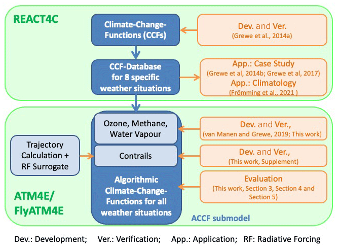
Figure 1Overview of conceptual development and relevant projects (i.e. REACT4C, ATM4E, and FlyATM4E) leading to the algorithmic Climate Change Functions (aCCFs) and the ACCF submodel.
The individual CCFs, the basis of the aCCFs, were developed slightly differently. The CCFs of O3, CH4, and H2O were calculated using a well-established modelling chain within EMAC (Jöckel et al., 2006, 2010). The model follows a multi-step approach starting with the simulation of the fate of emissions. The impact of pulse emission from a large number of time–region grid points is efficiently calculated by applying a Lagrangian transport scheme (i.e. following the air parcel). The RF caused by these pulse emissions is computed using the online diagnostic of the EMAC radiation scheme. Grewe et al. (2014a) and Frömming et al. (2021) have described details of this approach.
For the contrail CCF, the Lagrangian trajectories were used to determine the lifetime of a contrail, the temperature, and the position along the lifetime of a contrail. The Lagrangian trajectories were computed using the ECMWF reanalysis data (ERA-Interim; Dee et al., 2011) with winds input to a trajectory model (Methven, 1997). Accordingly, the contrail optical depth and solar zenith angle were calculated to obtain the contrail RF. The main discrepancy between contrail CCF and the other CCFs lies in the RF calculation. The contrail RF is calculated using the parametric model described by Schumann et al. (2012), which is different from the EMAC radiation scheme. Knowing the RF, to obtain the ATR20 value, the conversion from RF to ATR20 is calculated using the climate response model AirClim (Grewe and Stenke, 2008; Dahlmann et al., 2016) in a consistent way for all species considered, which was not the case in the earlier studies.
Based on the CCFs, the regression method was then applied to derive the aCCFs of O3, CH4, H2O (van Manen and Grewe, 2019), and the contrail cirrus aCCFs (Supplement of this paper). The CO2 aCCF is a constant value, which is determined based on emission scenarios. Note that the values from van Manen and Grewe (2019) and Irvine et al. (2017, Supplement to this publication) are updated by the formulas in the present study, as a more consistent conversion to ATR is employed, using slightly different response functions and consistent future scenarios for all species.
3.1 Model description EMAC
ACCF 1.0 is a submodel of the global atmospheric-chemistry model EMAC. EMAC is a numerical chemistry–climate model system that includes submodels describing the tropospheric and middle atmosphere processes and their interaction with oceans, land, and influences from anthropogenic emissions (Jöckel et al., 2010). It uses the second version of the Modular Earth Submodel System (MESSy2 version 2.53; Jöckel et al., 2010) to connect computer codes generated from different institutions. The core atmospheric model is the fifth-generation European Centre HAMburg general circulation model (ECHAM5 version 5.3.02; Röckner et al., 2006). The model resolution used in the current study is T42L31ECMWF, corresponding to 2.8∘ by 2.8∘ in latitude and longitude and 31 vertical hybrid pressure levels up to 10 hPa. The temporal resolution is 12 min.
3.2 Submodel ACCF 1.0
Figure 2 illustrates the structure of ACCF 1.0 and its interactions with other EMAC submodels. The ACCF 1.0 includes two layers: the sub-model interface layer (SMIL) and the submodel core layer (SMCL). The SMIL manages model input–output through the CHANNEL submodel (Jöckel et al., 2010). The SMCL is independent of other submodels and contains the code to solve the relevant equations for the individual aCCFs. The input variables to calculate aCCFs in the ACCF submodel are either from the base model calculation (i.e. temperature, geopotential) or from the other EMAC submodels. For instance, the H2O aCCF is a function of potential vorticity (PV) provided by the submodel TROPOP (Jöckel et al., 2006). The daytime contrail aCCF depends on the outgoing longwave radiation (OLR) at the top of the atmosphere from the submodel RAD (Dietmüller et al., 2016). The potential contrail coverage (potcov) calculated from the submodel CONTRAIL (Frömming et al., 2014) is used to determine whether persistent contrails can form and may lead to a climate impact by contrails. The Supplement of this paper includes a user manual of the submodel ACCF. It describes the namelist settings of the ACCF submodel and includes submodels necessary for coupling input–output variables.
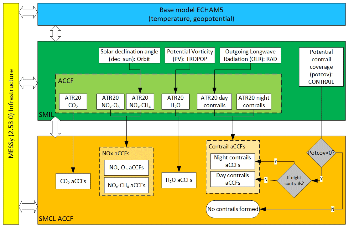
Figure 2Overview of EMAC/ACCF submodel structure, the calculation process in the ACCF submodel, and its interaction with the other MESSy submodels. SMIL (submodel interface layer) and SMCL (submodel core layer) are components of MESSy coding standards.
3.3 Basic mechanisms of submodel ACCF 1.0
This section summarizes the formulas of aCCFs 1.0. For full details of the original derivation, the reader is referred to van Manen and Grewe (2019) and the Supplement of this paper. The complete set of the aCCFs 1.0 computes the ATR20 of CO2 emissions, H2O emissions, NOx emissions (forming O3 and decreasing CH4 + PMO), and day/night contrail cirrus.
3.3.1 Synoptic on a selected day
The individual non-CO2 aCCFs depend on weather parameters, e.g. temperature, geopotential, and potential vorticity. A 1 d simulation on 18 December 2015 was performed to demonstrate such correlations. Figure 3 shows the geographical distribution of (a) temperature, (b) potential vorticity, and (c) geopotential over Europe at the pressure level of 250 hPa on the same day. These parameters are calculated by running the EMAC model nudged towards the ERA-interim data and will be used to calculate the non-CO2 aCCFs (see the following sections).
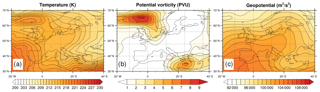
Figure 3Geographical distribution of (a) temperature (K), (b) potential vorticity in standard potential vorticity units (PVUs; 1 PVU = 10−6 K m2 kg−1 s−1), and (c) geopotential (m2 s−2) over Europe at 250 hPa on 18 December 2015.
3.3.2 CO2 aCCF
CO2 is a long-lived species, and hence, the climate impact of aviation's CO2 depends only on the amount of CO2 emitted. Therefore, the CO2 aCCF is calculated using the nonlinear climate–chemistry response model AirClim, assuming a 1 Tg fuel use in 2017. The CO2 aCCF then represents the average temperature response of CO2 for 2017–2036 (in K (kg (fuel))−1) (named P-ATR20). As a result, a constant value of K (kg (fuel))−1 was obtained. For the same amount of emission in 2017, but with an annual growth rate according to a business-as-usual (BAU) future scenario as given by Grewe et al. (2021), the ATR20 for CO2 (named F-ATR20) was K (kg (fuel))−1. A conversion factor of 9.4 was derived from the P-ATR20 to F-ATR20.
3.3.3 NOx-induced aCCFs
The aviation NOx emission (NOx= NO + NO2) leads to O3 formation via a catalytic reaction. NO reacts with HO2 forming NO2. Due to photodissociation, NO2 forms O(3P), leading to the O3 formation. The O3 formation, on the other hand, enhances the OH production (e.g. Grewe et al., 2017a), hence causing a shift of the ratio towards OH. The additionally formed OH leads to the oxidation of CH4.
Furthermore, the destruction of CH4 leads to a reduced O3 production rate as feedback to the O3 concentration. This O3 change is called primary mode ozone (PMO) (Wild et al., 2001). The effect of PMO is much smaller than the initial O3 production. However, PMO has a longer lifetime (is bound to the CH4 perturbation) than the initial O3 production. Furthermore, because of the CH4 oxidation, less CH4 enters the stratosphere, which again reduces the SWV. Since H2O is a greenhouse gas, the decrease in SWV reduces the warming effect of H2O (Myhre et al., 2007). The overall aviation-induced NOx effects include the short-term O3 increase and long-term CH4 reduction (also CH4-related PMO and SWV decrease). The current NOx aCCF addresses the impact of short-term O3 production and CH4 destruction and PMO reduction. SWV decrease is not taken into account because of its low magnitude. The corresponding formulas are presented below.
NOx-induced O3-aCCF
Earlier research showed the impact of weather patterns and related transport processes on the contribution of aviation NOx emissions to O3 and CH4 concentrations (Grewe et al., 2017c; Frömming et al., 2021; Rosanka et al., 2020). For instance, Grewe et al. (2017c) and Frömming et al. (2021) showed that a unit NOx emission within a high-pressure blocking situation leads to more O3-induced RF than a NOx emission west of this high-pressure area because the transportation pathways differ significantly. Air parcels starting within the high-pressure system are transported to the tropics and lower altitudes, experiencing a more active chemical regime and faster O3 production (Rosanka et al., 2020).
The analysis by van Manen and Grewe (2019) independently looked at correlations of CCF data describing the atmospheric state (meteorological and chemical data) at the time of emission. They found the best correlation representing the impact of ozone changes caused by a local NOx emission with the geopotential and temperature. This indicates that the weather regime at the time of emission essentially controls the air parcel's fate in which NOx is emitted. Thereby, the O3-aCCF (in K (kg (NO2))−1) is developed based on temperature (T) (in K) and geopotential (Φ) (in m2 s−2). For an atmospheric location at time t with and , the O3-aCCF can be found in Eq. (1). Please note that the coefficients in Eq. (1) differ from those derived in van Manen and Grewe (2019) in order to have a consistent set of formulas representing ATR20 for a pulse emission scenario (P-ATR20). Based on this, other metrics, for instance, ATR20 for future emission scenarios (F-ATR20), can be derived (e.g. Table 1). For the same reasons, corrections are also applied for coefficients of methane formulas (Eq. 2) and water vapour formulas (Eq. 5).
where P-ATR20 is the ATR20 for a pulse emission.
Figure 4a shows an example of the O3-aCCF (in K (kg (NO2))−1) on 18 December 2015 over Europe at 250 hPa. The contour lines indicate the geopotential, and it is noticeable that the O3-aCCF strongly follows the geopotential distribution. Overall, the changes in O3 concentration caused by NOx emissions have warming effects.
NOx-induced CH4-aCCF
The analysis by van Manen and Grewe (2019) showed the highest correlation of the CH4 response to NOx emissions with geopotential and the mean incoming solar radiation, i.e. combining the initial transportation pathway with an indicator for both seasons and available incoming radiation. Therefore, the CH4-aCCF (in K (kg (NO2))−1) is based on geopotential (Φ) (in m2 s−2) and incoming solar radiation at the top of the atmosphere as a maximum value over longitude (Fin) (in W m−2). For an atmospheric location at time t with , the CH4-aCCF can be found in Eq. (2).
where P-ATR20 represents the ATR20 for pulse emission, and Fin is calculated by Eq. (3).
where S is the total solar irradiance; θ is the solar zenith angle; φ is latitude; and d is the declination angle, defined by the time of year via the day of the year N.
NOx-induced PMO-aCCF
The effects of PMO and SWV decrease are not included in Eq. (2) but might be simply regarded as an offset of the CH4-aCCF with a linear scaling factor (e.g. Skowron et al., 2013), as they are primarily driven by the CH4 change. Here we apply a constant factor of 0.29 to the CH4-aCCF calculated in Eq. (2) to account for the PMO effect (Dahlmann et al., 2016). The PMO-aCCF is then described by Eq. (4).
Figure 4b shows an example of the combined CH4-CCF and PMO-aCCF (in K (kg (NO2))−1) on 18 December 2015 over Europe at 250 hPa. The overlaid contour lines represent the geopotential on the same pressure level and time step. We can see that the decrease in CH4 concentration caused by NOx emissions has cooling effects. Here, the cooling effects are overcompensated by the warming effects of O3. The overall effects of NOx emissions are expected to be warming, as seen in Fig. 4c, which shows the summation of O3-aCCF, CH4-aCCF, and PMO-aCCF.
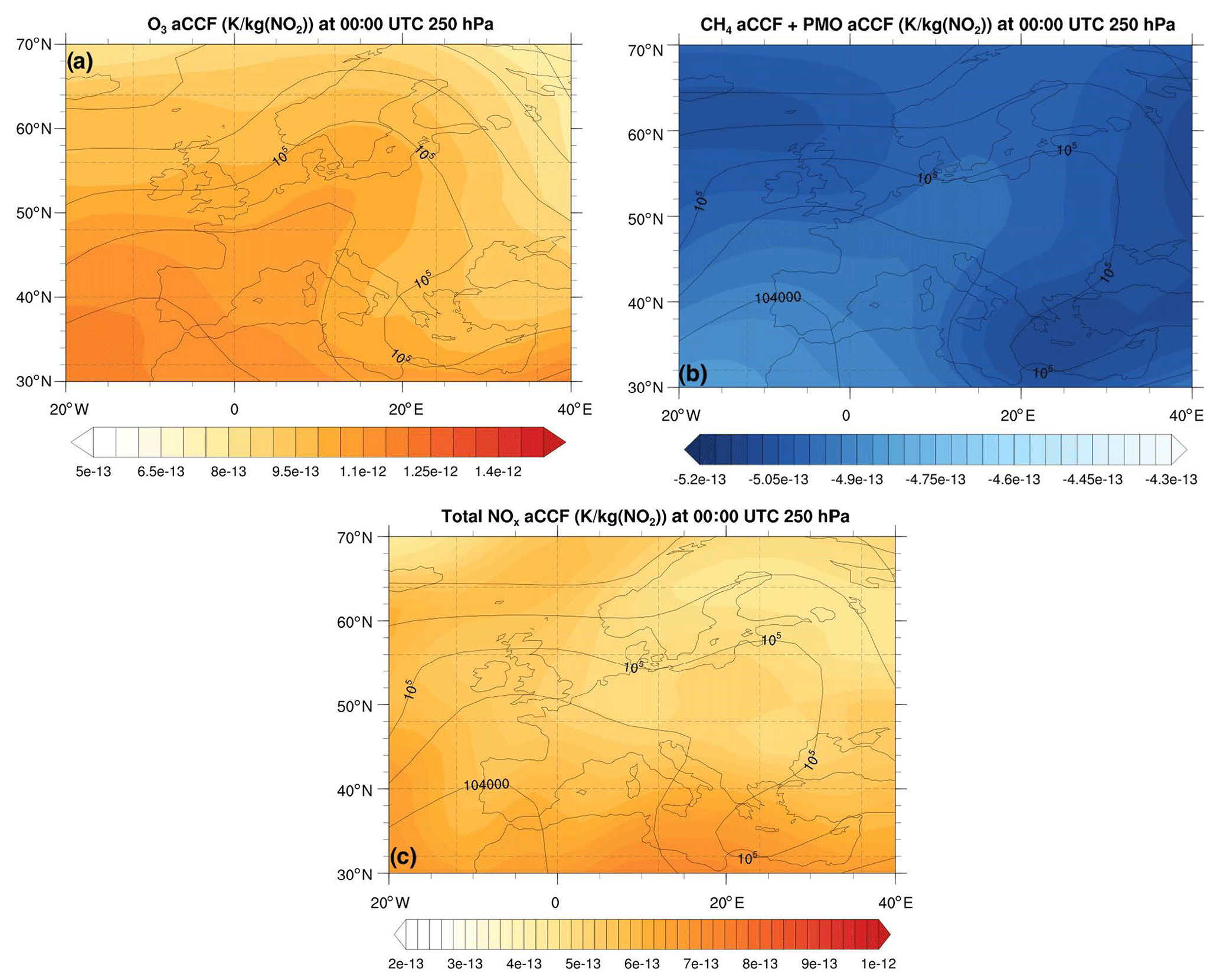
Figure 4NOx aCCF (in K kg (NO2)−1) on 18 December 2015 at 250 hPa for (a) O3-aCCF, (b) the combined CH4-aCCF and PMO-aCCF, and (c) the total NOx aCCF (O3-aCCF + CH4-aCCF + PMO-aCCF). The black contour lines are geopotential (in m2 s−2).
3.3.4 H2O-aCCF
The H2O emission's climate impact largely depends on its residence time. The likelihood of removing (rain-out) the emitted H2O decreases with altitude up to the tropopause. Or vice versa, the H2O emission's residence time increases with height and shows a sharp gradient at the tropopause (Grewe and Stenke, 2008; Wilcox et al., 2012). Hence the distance to the tropopause is already a good indicator of the H2O's lifetime. There are different tropopause definitions, for instance, temperature lapse rate (including the World Meteorological Organization (WMO), thermal tropopause, WMO, 1957) and potential vorticity (PV) (Kunz et al., 2011). The WMO thermal tropopause and the PV dynamical tropopause may differ locally (Grewe and Dameris, 1996). van Manen and Grewe (2019) showed that PV is a better indicator for the H2O-aCCF, since PV can also be used as a definition between tropospheric and stratospheric air masses.
The H2O-aCCF (in K (kg (fuel))−1) is based on PV in standard potential vorticity units (PVUs). For an atmospheric location at time t with , the H2O-aCCF can be found in Eq. (5).
Figure 5 shows an example of the H2O aCCF (in K (kg (fuel))−1) on 18 December 2015 over Europe at 250 hPa. One can notice that the H2O has warming effects in general, and the highest values occur at the location where the potential vorticity is also high (see Fig. 3b).
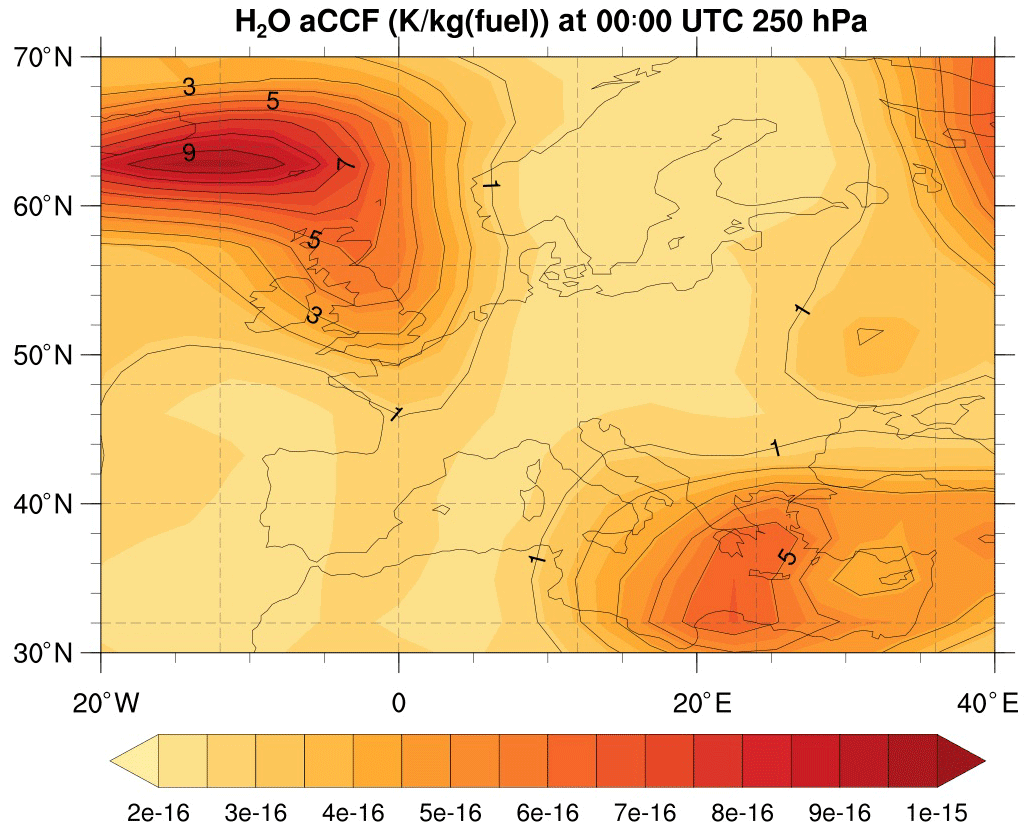
Figure 5H2O aCCF (coloured contour) (in K (kg (fuel))−1) and potential vorticity (black contour) (in standard potential vorticity units (PVUs)) on 18 December 2015, at 250 hPa.
3.3.5 Contrail cirrus aCCF
Contrail cirrus is short-lived. Because of its contrasting effects on shortwave and longwave radiation, contrail cirrus's radiative and climate effects distinguish between daytime and night-time. Thus, the specific radiative forcing of contrail cirrus (in W m−2) per flight distance has been developed for the daytime and night-time conditions by Emma Irvine (now Klingaman) based on reanalysis data (Klingaman and Shine; see Supplement). Note that, in the Supplement, the contrail coverage is assumed to be either 1 or 0, which is reasonable for higher horizontal resolutions. Therefore contrail distance equals flight distance in a grid box. Here, however, we deal with lower horizontal resolutions of T42 (Sect. 3.1), and the conversion of flight distance to contrail distance requires the multiplication of the potential contrail coverage value of the regarded grid box. This approach ensures that Grewe et al. (2014a) and the Supplement are consistent. Unlike the other aCCF formulas in calculating the P-ATR20 value directly, the algorithm of contrail cirrus estimates the global- and annual-mean specific RF per flight distance using the parametric equation of Schumann et al. (2012). Accordingly, the contrail-cirrus aCCF (an approximation of ATR20) for pulse emissions (P-ATR20contrail) is obtained as a product of the specific RF per flight distance value and a constant of 0.0151 K W m−2 derived using the AirClim model.
Night-time contrail aCCF
Night-time contrails refer to contrails with their entire (6 h in this paper) lifetime occurring at night. Since these contrails only exist during hours of darkness, they cause only longwave RF, so their net RF must be positive (warming). The scatterplot of relevant meteorological variables against the net RF of night contrails was used to identify which parameters had the strongest relationships with the net RF (see Klingaman and Shine; see Supplement). It was found that the local temperature can provide reasonable approximations for the night contrails' radiative effects. By using the nonlinear regression method, the specific RF per flight distance of night-time contrails (RFcontrails-night) (in W m−2 km−1) is derived based on temperature (T) (in K). For an atmospheric location at time t, with , the specific RF per flight distance of night-time contrail cirrus can be found in Eq. (6). Please note that correlation is not valid for temperatures less than 201 K. For temperatures below 201 K, the value should be set to 0.
By multiplying the factor of 0.0151 K W m−2, the night-time contrail aCCF (in K per flown km) is calculated in Eq. (7). As explained in Sect. 2, the conversion factor from specific RF to ATR20 for contrails is obtained using the climate response model, AirClim (Grewe and Stenke, 2008; Dahlmann et al., 2016). We apply a consistent set of global emission inventory for a given scenario, for which the specific RF and ATR20 are calculated. The ratio between specific RF and ATR20 is then derived as 0.0151 K W m−2, hence used here as a conversion factor.
Daytime contrail aCCF
Daytime contrails refer to contrails that form and dissipate during daylight or have a part of their 6 h lifetime during the day. The specific RF per flight distance of daytime contrails (RFcontrails-day) (in W m−2 km−1) is based on the OLR (in W m−2) at the top of the atmosphere at the time and location of the contrail formation. Therefore, for an atmospheric location (x,y) at time t with , the RF of daytime contrail cirrus can be found in Eq. (8). Please note that Eq. (8) will predict negative specific RF per flight distance for OLR W m−2 and positive specific RF per flight distance for any larger OLR values.
Similarly, the daytime contrail aCCF in kelvin per flown kilometre is calculated in Eq. (9).
Please note that in the ACCF submodel, the contrail aCCF is only activated when the potential contrail coverage is larger than zero and the flight distance is converted to contrail distance by multiplying with the potential contrail coverage (see also above). Depending on the time of the contrail cirrus occurring, either day- or night-contrail-cirrus aCCF calculation is used.
Figure 6 shows an example of the day- and night-time contrail aCCF on 18 December 2015 over Europe at 250 hPa: (a) 12:00 UTC and (b) 00:00 UTC. One can see that the contrail aCCF depends on the formation time. For instance, at the exact location (e.g. over Ireland), a contrail formed at 12:00 UTC has a cooling effect, whereas at 00:00 UTC it has a warming impact.
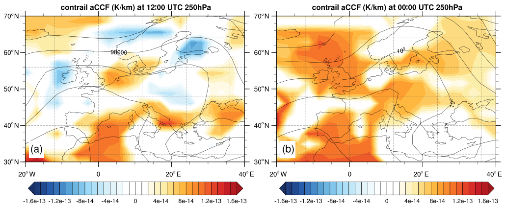
Figure 6Contrail-cirrus aCCFs (coloured contour) (in K km−1) and geopotential height (black contour) (in m2 s−2) on 18 December 2015 at 250 hPa: (a) 12:00 UTC and (b) 00:00 UTC.
3.4 Physical climate metric and efficacy applied in the ACCF submodel
The aCCF formulas provided in Sect. 3.3 calculate the climate impact of O3, CH4, PMO, H2O, and contrail cirrus consistently in P-ATR20, i.e. for a pulse emission. With pulse emission, one could compare, for instance, the future impact of emissions in a given year. When a non-pulse emission is considered, for example, an increased emission scenario representing the growth of air traffic, the metrics of pulse emission can be converted (Fuglestvedt et al., 2010).
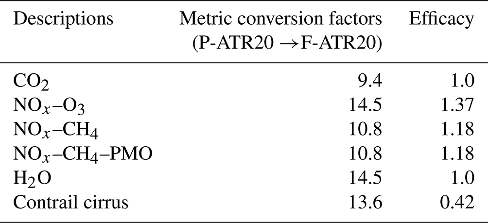
Here we demonstrate an example of converting the P-ATR20 to the ATR20 of the future BAU emission scenario (F-ATR20) derived by Grewe et al. (2021). We determined the climate metric conversion factors for the aCCFs of O3, CH4, PMO, H2O, and contrail cirrus using the AirClim model. We performed two simulations with pulse emissions in 2017 and future emission scenario BAU, respectively. For both simulations, we calculate the factor between ATR20 and RF for each effect and use the ratio between these values as conversion factors. Table 1 shows the conversion factors from the P-ATR20 to the F-ATR20 metric. In the namelist of the ACCF 1.0, these metric conversion factors can be changed depending on the chosen scenario for different purposes (see Supplement).
The efficacy of the individual forcing agents (O3, CH4, PMO, H2O, and contrail cirrus), which consider the different effects of these forcing agents in producing global temperature change (e.g. Hansen et al., 2005), are not included in the aCCF formulas in Sect. 3.3. However, they can be easily included via namelist settings of the ACCF submodel (see the user manual in the Supplement for namelist settings). The present study implemented the forcing efficacies in Lee et al. (2021), as shown in Table 1. The final output of the ACCF submodel is a product of the output of aCCF formulas in Sect. 3.3, the metric conversion factor, and the efficacies.
Table 1Example values of climate metrics conversion factors from ATR20 of a pulse emission in 2017 (P-ATR20) to ATR20 of future BAU emission scenario (F-ATR20) and efficacies of different species/contrail-cirrus effect. The efficacies are taken from Lee et al. (2021).
In this section, we present the application of the submodel ACCF, how it describes the climate effects of aviation emissions, and how it can be used for aircraft trajectory optimization. This section also presents the quality check of ACCF submodel outputs. Firstly, we compare the climatology of the prototype aCCFs for O3, CH4, H2O, and contrail cirrus to results from the literature. Secondly, we study the O3 RF change caused by the air traffic emissions through the AirTraf submodel calculated online for cost- and climate-optimized flights, respectively. The climate-optimized flights minimized the NOx-induced O3 effect computed using Eq. (1).
4.1 Climatology of aCCFs
The climatological aCCFs are calculated for all meteorological situations emerging over a 1-year nudged simulation in 2016. The climate metric conversion factors and the efficacies in Table 1 are considered. Figure 7a–c show the annual and zonal mean aCCF from O3, CH4 combined with PMO, and total NOx (O3 + CH4 + PMO), respectively. The considered region is over the Northern Hemisphere and between 150–300 hPa.
The warming effects of O3 increase with the altitude and towards the lower latitudes, which is in line with other studies. For instance, Fig. A2 of Dahlmann et al. (2016) shows that the global annual-mean RF of aviation NOx-induced O3 increases with the pressure altitude. Figure 8 of Grewe and Stenke (2008) shows the global mean temperature change of NOx-induced O3 for 2100, considering a constant emission from 2050–2100. Due to different emission scenarios, the absolute value in Fig. 7 of this study is much lower (orders of magnitude). However, when comparing the vertical and lateral variability in the vertical range of 150 and 300 hPa (typical flight corridor range), a similar pattern can be observed.
In comparison, the cooling effect of CH4 (including PMO) increases towards lower altitudes but shows less dependency on latitude than O3 at the lower altitude. That is to say, if the flight altitude is reduced, one would expect more substantial cooling effects due to NOx-induced CH4 depletion. Such phenomena are in line with the study of Frömming et al. (2012), where it was shown that the CH4 mean RF reduces when flying lower. Furthermore, when comparing Fig. 8 of Grewe and Stenke (2008) and Fig. A2 of Dahlmann et al. (2016) in the same vertical range, we notice some discrepancies in the CH4 aCCF pattern in the latitudinal directions. Both Figs. 8 and A2 show that the cooling effects of CH4 increase towards lower latitudes. This was also observed in Köhler et al. (2013). However, Fig. 7b shows an opposite trend, which needs further diagnosis in future studies. Since the value of CH4 aCCF is about 5 times smaller than the O3 aCCF, one can consider the mismatch of CH4 aCCF to be of minor importance.
Figure 7d shows the annual zonal mean H2O aCCF. The warming effects of H2O increase with altitude and towards the polar region, which matches well with the previous study of Grewe and Stenke (2008), confirming that ACCF accurately represents the variations in global climate change of aviation H2O emissions at the different regional locations and different altitudes.
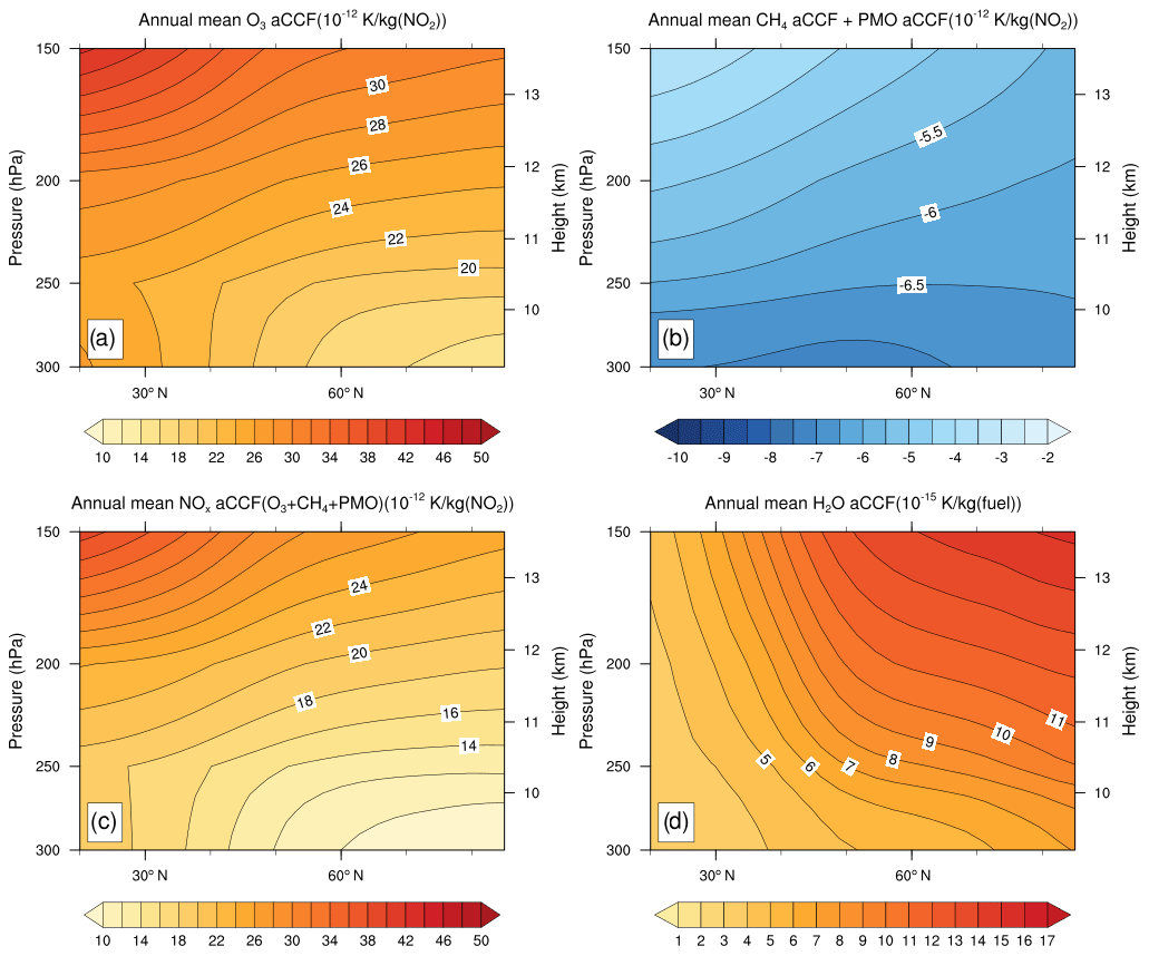
Figure 7Annual zonal mean aCCFs (F-ATR20) in the Northern Hemisphere and between 150 to 300 hPa attributed to (a) NOx–O3 effects; (b) NOx–CH4 (+PMO) effects; (c) overall NOx effects (O3+CH4+PMO); (d) H2O effects.
Figure 8 shows the zonal mean climatological value of contrail cirrus aCCFs (in K km−1) by combining the day and night effects. The RF and hence the F-ATR20 are calculated at the location where contrails could be formed. We compare the climatological contrail-cirrus aCCF with the values presented in the previous literature (Fig. A2 of Dahlmann et al., 2016, where the annual zonal mean contrails RF per flown km are calculated using normalized emissions). We notice that the order of magnitude and the profile of the contrail aCCF match the study of Dahlmann et al. (2016).
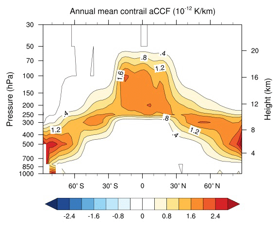
Figure 8Annual zonal mean contrail aCCF (F-ATR20) (in K km−2): combined effects of day and night contrails.
4.2 Radiative forcing calculation of aircraft emissions using EMAC submodels
To demonstrate the usage of the ACCF 1.0 in aircraft trajectory optimization considering non-CO2 climate effects, we use the O3 aCCF to calculate the RF due to aviation NOx-induced O3 by combining ACCF with AirTraf, TAGGING, and RAD (EMAC submodels). Figure 9 shows how an aircraft trajectory from the departure to the arrival airport is guided through climate-sensitive regions, described with the help of the ACCF submodel. Providing atmospheric perturbations in reactive species to the TAGGING submodel calculates associated ozone changes, and eventually, radiative impacts are characterized in the RAD submodel. For the demonstration, we optimize the flight trajectories of a subset of daily European flights concerning either minimum cost (simple operating cost option in the AirTraf submodel; Yamashita et al., 2020) or minimum climate impact from only the NOx-induced O3 effect. In two different simulations, the associated NOx emissions alter O3 concentrations and thus their RF differently. The hypothesis of the reduced RF in climate-optimized routes would prove the concept of the O3 aCCFs. For a more detailed study, the climate impact of aviation NOx emissions should be a combination of O3, CH4, PMO, and SWV decrease. Here we focus on the short-term O3 effect to better understand the particular feature of the O3 aCCF.
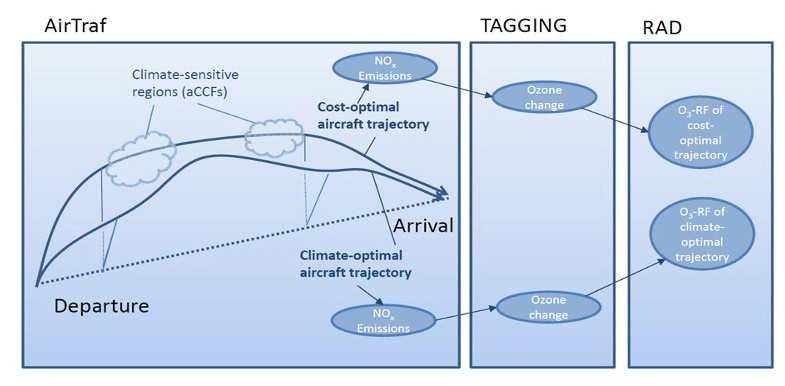
Figure 9Sketch of the radiative forcing calculations for ozone changes caused by online air traffic NOx emissions for cost- and climate-optimized flight trajectories. Cost-optimized aircraft trajectories minimize the simple operating cost of the flight, while climate-optimized aircraft trajectories minimize the climate impact (here only the NOx-induced O3 effect is included).
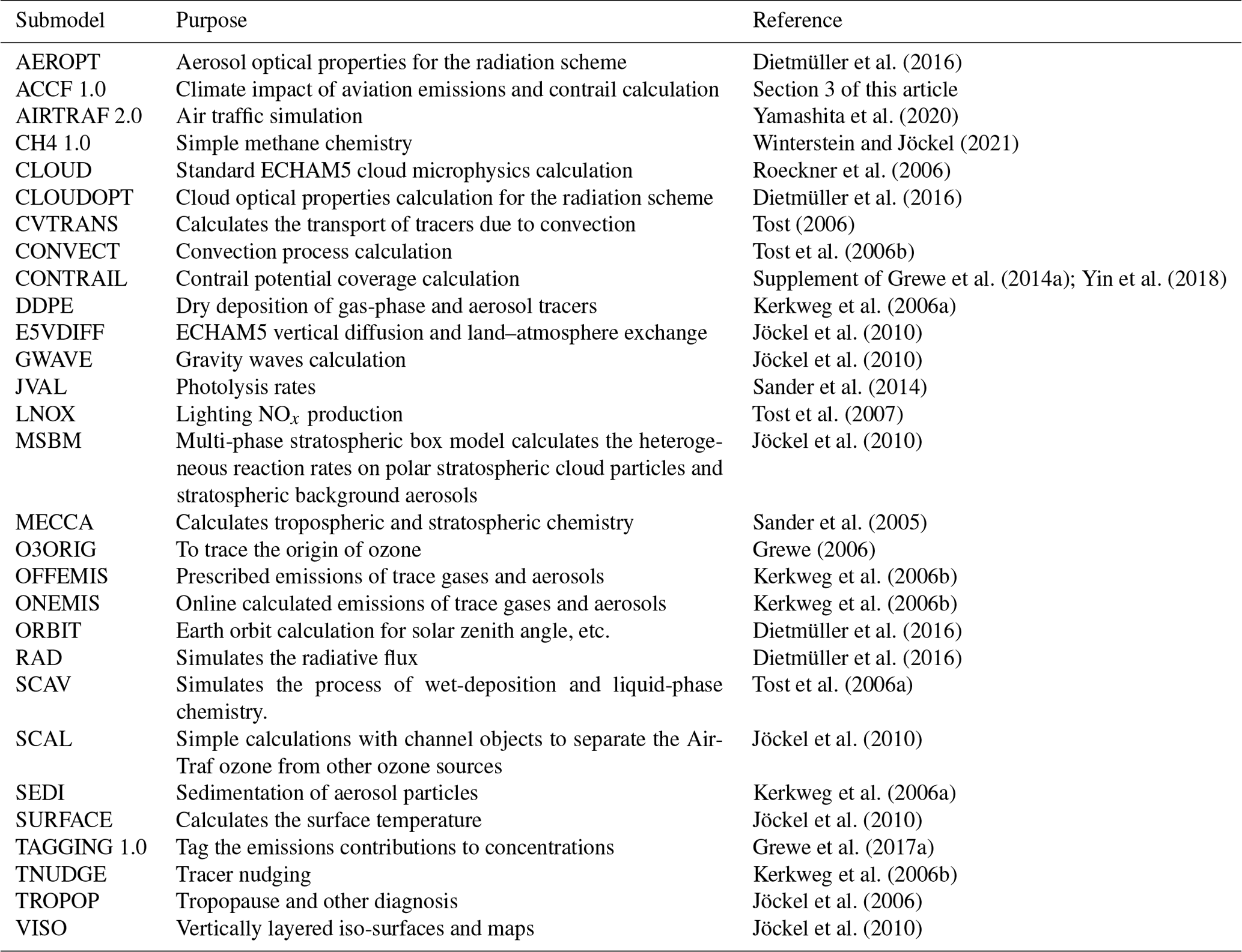
In line with the simulation scheme above, we configured the EMAC model with a list of EMAC submodels. In addition to the standard submodels, we use AirTraf 2.0 (Yamashita et al., 2020) to calculate the air traffic emissions from different flight trajectories, MECCA (Module Efficiently Calculating the Chemistry of the Atmosphere; Sander et al., 2005) and SCAV (SCAVenging; Tost et al., 2006a), to represent the chemical kinetics of EMAC. We also use TAGGING 1.0 (Grewe et al., 2017a) to tag the contributions of emissions to concentrations. The radiation flux change of the NOx-induced O3 change is calculated using the submodel RAD (Dietmüller et al., 2016). The complete list of used EMAC submodels in this simulation can be found in Table A1 of the Appendix.
The simulation setup for trajectory optimization is given in Table 2. A total of 85 daily European flights are used. The constant flight Mach number 0.82 combined with the wind speed will result in different ground speeds. For cost-optimized flight trajectories, simple operating cost calculated using Eq. (10) is the objective function. For climate-optimized flight trajectories, the F-ATR20 of NOx-induced O3 is used as the objective function. There are 11 design variables to express a flight trajectory. Five variables control the vertical change between flight levels of 8839 m (29 000 ft, FL290) and 12 497 m (41 000 ft, FL410), and six variables control the lateral shift. The Adaptive Range Multi-objective Genetic Algorithm (ARMOGA version 1.2.0, Sasaki and Obayashi, 2005; Sasaki et al., 2002) is implemented for trajectory optimization.
where t is the flight time in hours, mfuel is the fuel consumption in kilograms, Ct is the flight time related cost in euros (EUR) per hour, and Cf is the fuel related cost in EUR per kilogram of fuel).
Table 2AirTraf simulation setup for trajectory optimizations considering cost minimum and climate minimum (only NOx–O3 effect), respectively.
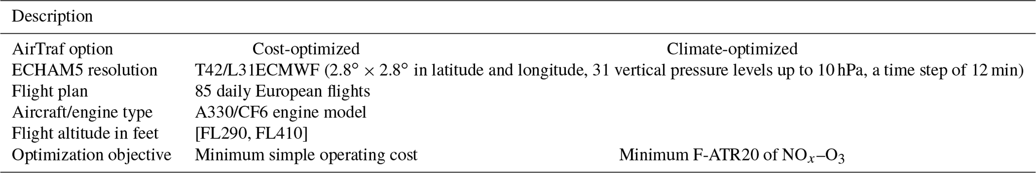
Figure 10 shows the calculated flight trajectories on a single day for the minimal cost (red) and the minimal NOx–O3 climate impact (green). Figure 10a shows the changes in flight altitudes, and Fig. 10b shows the lateral shifts of flight trajectories aggregated along the vertical direction. For cost-optimized flights, the aircraft tends to fly as high as possible within the vertical constraints to maximize aerodynamic efficiency, reducing fuel consumption and the associated operational cost. As for the climate-optimized routine, the situation is much more complicated. The climate impact of O3 attributed to NOx emissions depends on multi-criteria, e.g. the emitted quantity, time, location, and weather. On average, the altitudes of climate-optimized flights are lower than those of cost-optimized flights. We also notice from Fig. 10b that some flights tend to shift northward to reduce the NOx–O3 climate impact.
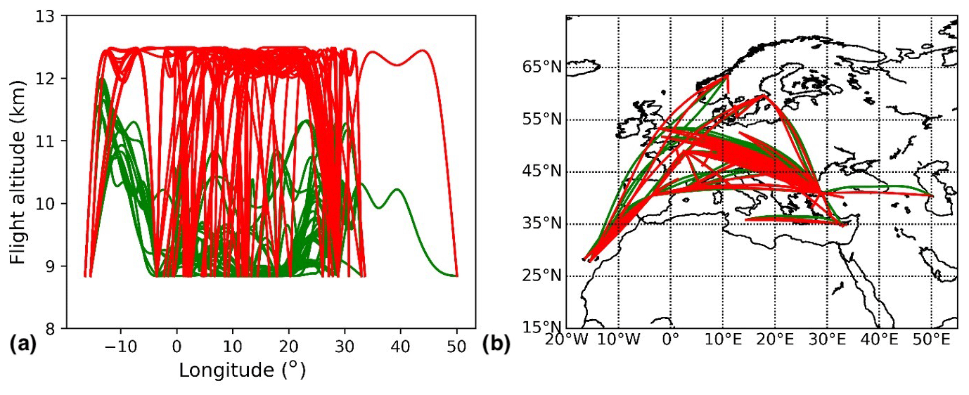
Figure 10Calculated daily flight trajectories in (a) vertical variation and (b) lateral variation using AirTraf for cost-optimized (red) and climate-optimized flights considering only the NOx–O3 effects (green).
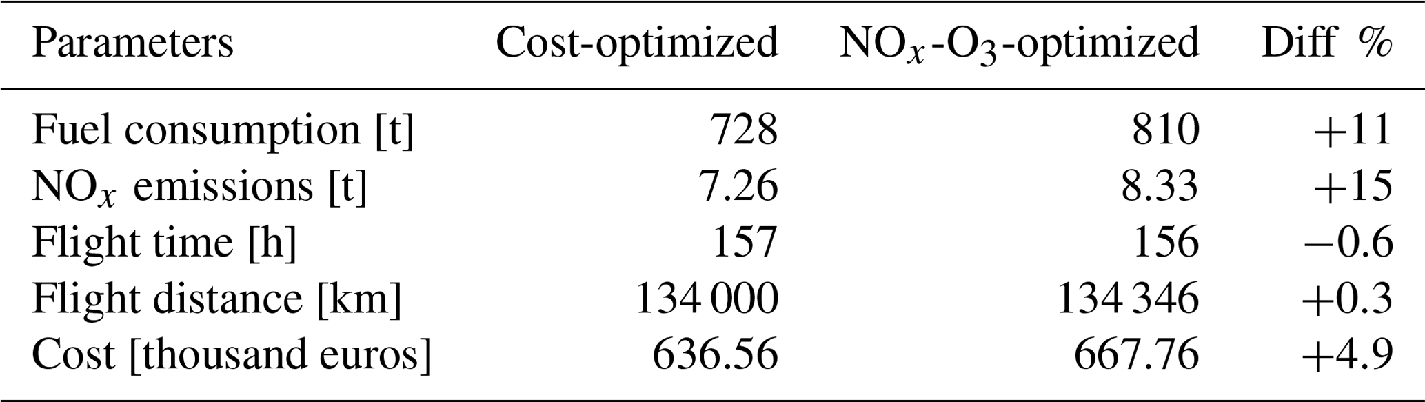
The flight characteristics and performance data are summarized in Table 3. Compared to the cost-optimized flights, the fuel consumption of the climate-optimized flights is 11 % higher, and the NOx emissions are 15 % higher. The total cost of climate-optimized flights is about 5 % higher than that of cost-optimized flights.
Table 3Daily sum over the flight-plan of the characteristics of the cost-optimized and the NOx–O3-optimized flights.
Having the flight trajectories and their respective performance calculated with AirTraf using ACCF values (Fig. 10), NOx emissions from cost- and climate-optimized trajectories are then integrated into the global EMAC model as tagged species by the EMAC/TAGGING submodel. This allows the contributions of different NOx emission sources to the atmospheric changes of the NOx and O3 concentrations to be identified. This showcase simulation using tagging chemistry was run for 3 months, from January to March 2016. Figure 11 shows relative changes in monthly mean mixing ratio distribution of (a) NOx (in mol mol−1) and (b) O3 (in mol mol−1), comparing effects caused by NOx emissions from climate-optimized flight trajectories with the effect of cost-optimized trajectories (baseline) in March 2016. The figure is presented in the vertical cross-section. The climate-optimized trajectories emit NOx at a lower altitude than the cost-optimized trajectories; therefore, we see an increase in the NOx mixing ratio at the lower altitude (indicated by the red colour in Fig. 11a). As a result, the O3 production is shifted downwards (see Fig. 11b). The residence time of O3 at the lower altitude is shorter due to a more efficient wash-out. Therefore, the calculated RF of the NOx-induced O3 for the climate-optimized flights (13.3 mW m−2) is about 2 % less than that of the cost-optimized flights, which confirms that the climate-optimized flight trajectories based on the O3 aCCF reduce the associated NOx–O3 climate effect.
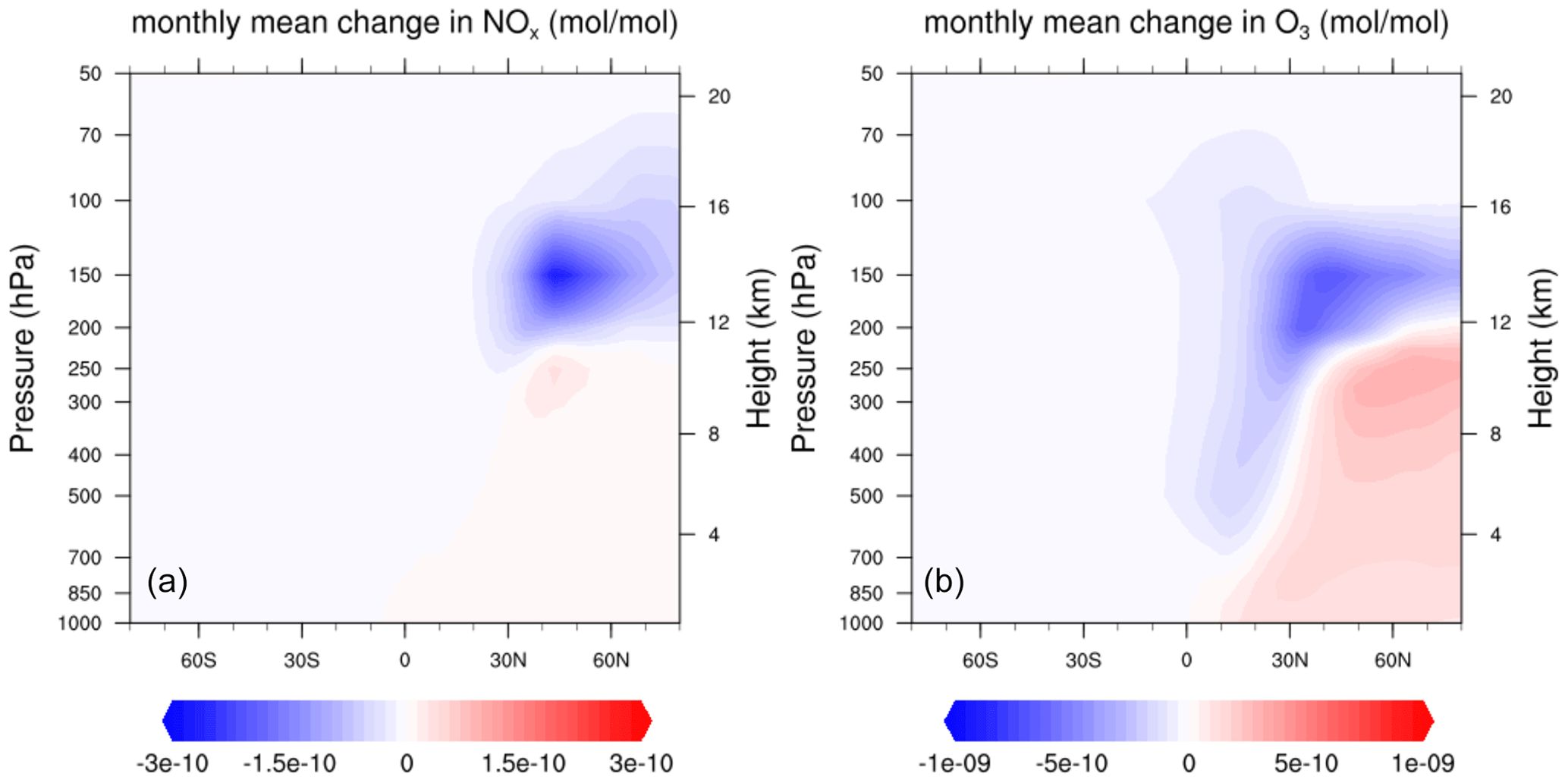
Figure 11Changes of (a) NOx mixing ratio and (b) resulting changes in O3 mixing ratio caused by NOx–O3-optimized flight trajectories using only O3 aCCF. The baseline is cost-optimized flights.
This section demonstrates the application of the ACCF submodel to assess the aviation climate effects during trajectory optimization. In previous research, Yamashita et al. (2020) implemented the ACCF submodel in AirTraf 2.0 to obtain climate-optimized trajectories. Here, we update the ACCF submodel outputs using the physical climate metric F-ATR20 and consider the efficacy of radiative effects.
5.1 Simulation setup
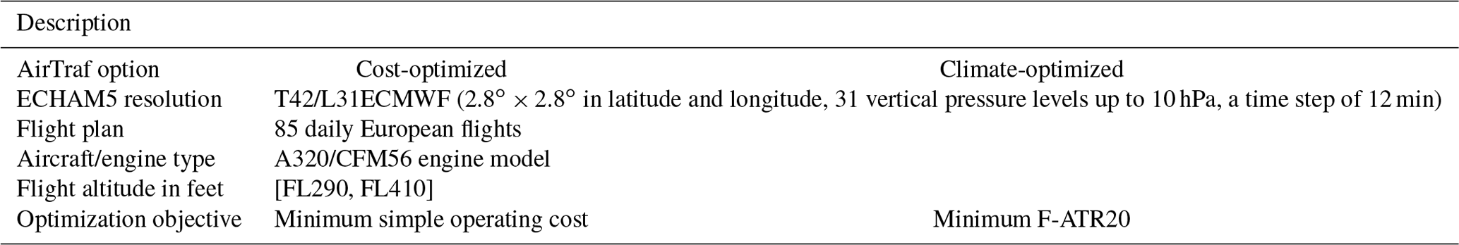
We couple the ACCF 1.0 with the AirTraf 2.0 in this simulation. In AirTraf 2.0, two optimization objectives are considered, respectively: cost- and climate-optimized. The simulation setup can be seen in Table 4. In this section, the climate-optimized trajectory minimizes the total F-ATR20 of CO2, NOx (summation of O3, CH4, and PMO), H2O, and day/night contrail cirrus, including the efficacies of individual species/contrail cirrus as shown in Table 1.
Table 4AirTraf simulation setup for trajectory optimizations considering cost minimum and climate minimum.
5.2 Optimized flight trajectories
We compare the F-ATR20 values of cost-optimized (red) and climate-optimized (green) trajectories in Fig. 12. Cost-optimized trajectories are characterized by higher flight altitudes to maximize aerodynamic efficiency, which is similar to what was described in Sect. 4.2. On the other hand, climate-optimized trajectories considering non-CO2 effects fly at lower altitudes at most locations to reduce the impact of the total NOx, H2O, and contrails.
Table 5 summarizes the flight characteristics. Compared to the cost-optimized flights, the climate-optimized trajectories (ignoring economic costs while only minimizing climate effects) tend to increase fuel consumption by 17 % and NOx emissions by 25 %. On the other hand, the total F-ATR20 is reduced by 51 % driven by the contrails effect (−89 %), followed by the combined CH4 and PMO impact (−41 %). The impact of CO2 and H2O is characterized by lower orders of magnitude than the impacts from NOx emissions and contrails; therefore, they are not crucial properties during the optimization process, but they are affected by changes due to higher fuel consumption (causing higher CO2 impact (+17 %)) and lower mean flight altitudes (leading to lower H2O impact (−33 %)).
Furthermore, one can observe that the contribution of CO2 to the overall climate impact is relatively low compared to the non-CO2 effects. This could be caused by choice of the physical climate metric and the radiation scheme used to develop the original CCFs and the following aCCFs characteristics. While ongoing research investigates how to best define an adequate climate metric reflecting short-term and long-term effects to a certain extent, we expect to develop a better understanding with further diagnosis.
Table 5Daily sum of flight characteristics over the cost-optimized and the climate-optimized trajectories on 18 December 2015.
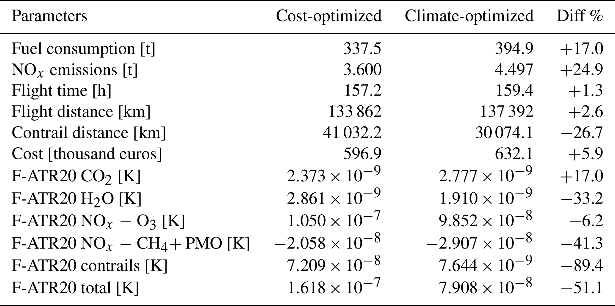
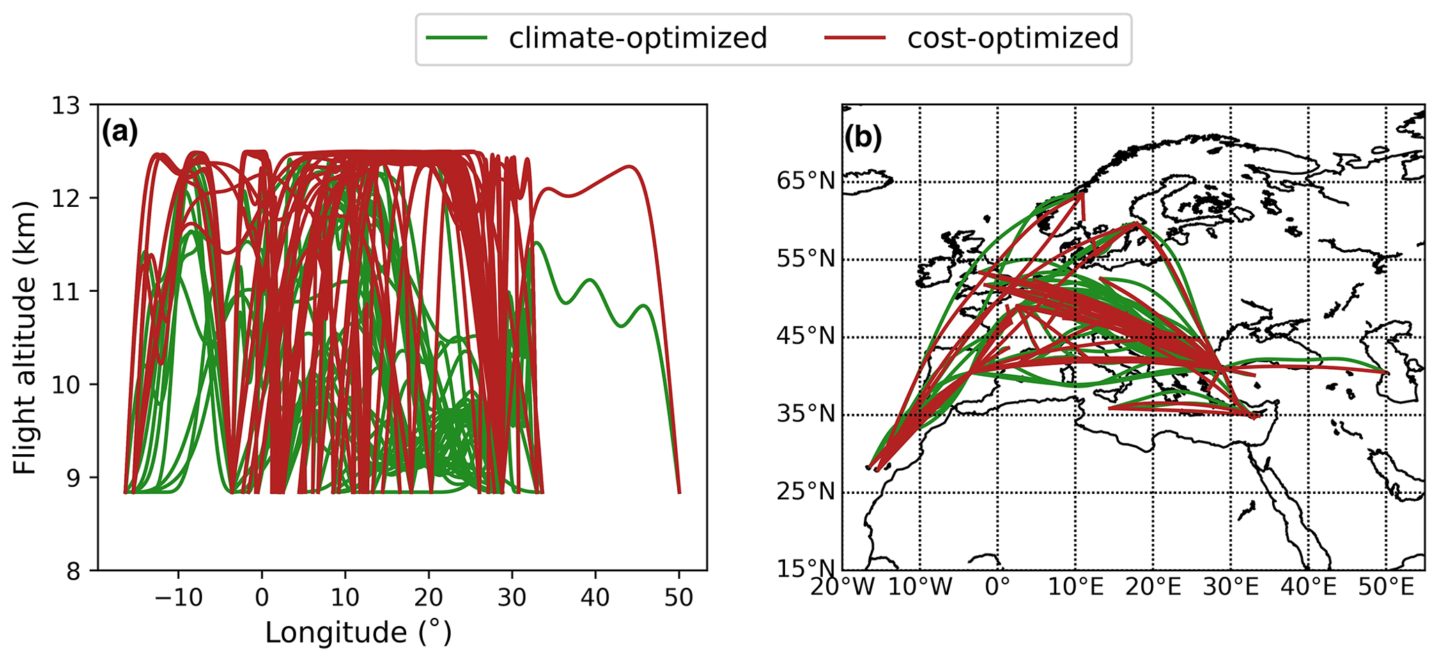
Figure 12Comparison of (a) vertical shift and (b) lateral shift between cost-optimized (red) and climate-optimized (green) trajectories on 18 December 2015.
This research implements a consistent set of prototype algorithmic climate change functions as the submodel ACCF 1.0 of EMAC, enabling quantifying aviation emission climate effects. The demonstration simulations confirm that the developed aCCFs can predict the characteristic patterns of ATR20 from H2O, NOx-induced O3, and contrail cirrus. The NOx-induced CH4 pattern shows a slight discrepancy in terms of latitudinal variabilities when compared to previous studies (Grewe and Stenke, 2008; Frömming et al., 2012; Köhler et al., 2013). As the total NOx aCCF is dominated by the positive O3, we expect that the combination of O3 and CH4 captures the feature of aviation NOx adequately. Further development of the CH4 aCCF formula is required to address the latitudinal discrepancy.
Furthermore, the ACCF submodel has been implemented in a comprehensive tagging chemistry simulation chain to evaluate mitigation gains because of modified aviation emissions. By coupling the ACCF submodel with the AirTraf submodel, NOx emissions are calculated from cost-optimized and climate-optimized flights considering only the NOx-induced O3 effect. The NOx emissions are then fed into the tagging chemistry scheme to estimate the resulting RF due to changes in O3 mixing ratios. The results confirmed that the climate-optimized trajectories reduce the RF of O3 by 2 % compared to the cost-optimized flights.
The case study on trajectory optimization for cost- and climate-optimized flights indicates a relatively low contribution of CO2 to the overall climate impact compared to the non-CO2 effects. Our first thoughts are that this might be related to the metrics we are using, the radiation scheme in developing the original CCFs models, and the regional effects. Ongoing work in the metric diagnosis and the geographical analysis will help us better understand the reasons.
6.1 Climate metrics conversion
Regarding the physical climate metric used in this study, the aCCF formulas in Sect. 3 calculate the average temperature response over 20 years for a pulse emission (P-ATR20). Based on the P-ATR20, it is possible to obtain different physical climate metrics for any other emission scenario by applying a climate response model, for example, AirClim. Though the flexibility of the ACCF namelist setup allows the user to convert the climate metrics, the metric selection involves different factors, for example, the perspective question (Fuglestvedt et al., 2010; Grewe and Dahlmann, 2015). We want to stress that we consider it essential that any optimization study carefully defines the physical climate metric used, the type of strategic decision envisaged, constraints given, and assumptions on policy and regulations accepted. For instance, one should identify the application scenario (or the perspective question) as the specific application scenario is critical for defining the adequate reference, the physical climate metric, and the emission scenario. A pulse emission would compare the future climate impact in a given year. A future emission scenario would compare the effect of varying emissions over a period in the future. From the perspective question, an adequate climate indicator and time horizon can then be deduced.
6.2 Uncertainties of contrail aCCFs
While the aviation-induced contrail-cirrus effects play essential roles in aviation's climate impact, the level of scientific understanding on contrail cirrus climate effects is moderate or low (see, for example, Lee et al., 2021), which implies a large uncertainty. The uncertainties of contrail-cirrus climate impact are subject to different aspects, including the natural variability of the atmosphere and modelling uncertainties. Both uncertainties propagate to contrail-cirrus aCCF.
For instance, contrail aCCF is only calculated when potential contrail coverage (potcov) is greater than zero. The potcov varies strongly with the local atmospheric temperature and relative humidity over ice, which again depend on specific models (e.g. an Earth system climate model vs. a weather forecast model with higher resolution). While comparing the temperature field calculated from the EMAC model on 18 December 2015 nudged towards the ECMWF reanalysis data (ERA-Interim) with the original ERA-Interim datasets at three pressure levels of 200, 250, and 300 hPa, we observed that the temperature calculated from the EMAC model is on average 3 K lower than the reanalysis data. This temperature difference affects the predicted potcov and the calculated contrail-cirrus aCCF (see Eq. 6). Figure 13 shows a comparison between the values of F-ATR20 calculated from contrail-cirrus aCCF on 18 December 2015 at 250 hPa. Figure 13a shows the geographical pattern using the original EMAC temperature, and Fig. 13b shows the geographical pattern when artificially correcting the 3 K temperature bias from the EMAC temperature. Two effects are observed: (1) the areas where the contrails might form are reduced for a warmer temperature, and (2) the maximum value of ATR20 increases indicating a more substantial warming effect. From this preliminary analysis, we could see that the uncertainties related to the inputs of aCCFs play an essential role in the robustness of the aCCFs results.
Furthermore, for a given model resolution, one might expect a latitude dependency of contrail aCCF as the flight distance per grid box varies with latitude, which is currently under investigation.
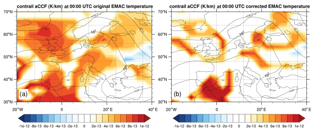
Figure 13Geographical distribution of contrail aCCF (in K km−1) on 18 December 2015 at 250 hPa for (a) the original EMAC temperature and (b) the bias-corrected EMAC temperature.
6.3 Ongoing research on the robustness of aCCFs
The aCCFs 1.0 used in this study represent a prototype formulation and face different aspects of uncertainties. The aCCFs are based on simulations performed for the North Atlantic Flight Corridor during summer and winter. While applying the aCCFs at European airspace, we observe that the climatological pattern of aCCFs in vertical and latitudinal variability matches other studies (Dahlmann et al., 2016). Nevertheless, using them at other locations and seasons should be done cautiously and carefully evaluated. We would like to note here that the development of the aCCFs is an ongoing research activity, and an expansion of their geographic scope and seasonal representativeness is under investigation.
Furthermore, a concept toward robust aCCFs is under development, which will additionally integrate information about uncertainties arising from low-level understanding of climate science (Matthes et al., 2023). This robust aCCFs will rely on a set of aCCFs that consider educated guess estimates of individual climate impacts. The basis of this educated guess can be, for example, the conservative estimates of the individual RF (see Lee et al., 2021). Additionally, the second set of aCCFs will be provided to perform individual risk analyses originating from different sources of uncertainty. This will be done by quantitatively estimating the error if a lower or higher climate impact is assumed. With that, we add up to low- or high-range aCCF estimates, respectively. This concept of robust aCCFs can be applied in aircraft trajectory optimization studies with EMAC/AirTraf. The corresponding experiment design would rely on one reference optimization using the educated guess aCCFs and sensitivity optimization experiments using the low- or high-range aCCFs estimates. A robust trajectory would be characterized by not losing overall benefits (mitigation gains) even if lower or upper estimates of aCCFs are applied. Technically, this could be solved by calling the ACCF submodel several times within the same simulation, using the range of different aCCFs estimates.
We developed the submodel ACCF 1.0 of the chemistry–climate model EMAC to estimate the climate impact of aviation emissions in the flight corridor of the Northern Hemisphere, representing an implementation of aCCF 1.0 formulas. The submodel ACCF 1.0 was developed according to the MESSy standard and was thoroughly presented in this paper. This submodel calculates aviation's climate impact of CO2 emissions and non-CO2 effects, such as from NOx-induced O3, NOx-induced CH4 (including PMO), H2O, and contrail cirrus based on a consistent set of aCCFs. The mathematical formulation of the individual prototype aCCFs 1.0 is provided.
The climatological profile of the NOx-induced effect on ozone (O3 aCCF) shows that the warming effects of NOx-induced O3 increase with altitude between 150–300 hPa and towards lower latitudes, while the climatological distribution of H2O aCCF shows that the warming effect of H2O increases towards higher altitudes or latitudes. By comparison to the literature, we conclude that the vertical and latitudinal structure within the flight corridor of the Northern Hemisphere of the NOx-induced O3 and H2O is well represented by the aCCFs.
The NOx-induced effect on methane (CH4 aCCF) shows that cooling effects increase towards lower altitudes and higher latitudes. Although the latitudinal variation of CH4 aCCFs is less pronounced than for other species, it is somewhat of the opposite tendency to the literature. Since the absolute value of CH4 aCCF is mostly overcompensated for by the O3 aCCF, the total NOx aCCF could still capture the vertical and latitudinal variability of the overall NOx effects.
For the contrail-cirrus aCCF, the climatological pattern follows the potential contrail coverage. The calculated F-ATR20 value also matches the literature, except that contrail-cirrus aCCF generates values at low altitudes where contrails are not expected to be formed. This might be related to the threshold of temperature and humidity used for calculating the potential contrail coverage and the temperature bias in the EMAC model.
Using the tagging chemistry approach, we were able to show that climate-optimized trajectories based on O3 aCCF indeed reduce the radiative forcing contribution from aviation NOx-induced O3 compared to the cost-optimized trajectories.
Finally, the trajectory optimization results confirm that the total F-ATR20 of climate-optimized flights is about 51 % lower than the cost-optimized flights, with the largest contribution from contrail cirrus.
Table A1Summary of MESSy submodels used in the chemistry simulation.
ACCF 1.0 has been published for the first time as a submodel of the Modular Earth System Submodel System (MESSy) since version 2.53. MESSy is continuously further developed and applied by a consortium of institutions. The usage of MESSy and access to the source code are licensed to all affiliates of institutions members of the MESSy Consortium by signing the MESSy Memorandum of Understanding. More information can be found on the MESSy Consortium website (http://www.messy-interface.org, MEESy, 2023). The version presented here corresponds to ACCF 1.0. The status information for ACCF will be available on the website.
The dataset used in this study is available in the 4TU.ResearchData repository at https://doi.org/10.4121/bea8a3fe-e34c-4598-9f94-c5a5c63348e5 (Yin et al., 2023).
The Supplement related to this paper includes the development of contrail-cirrus aCCF and the user manual for the ACCF submodel setup. The supplement related to this article is available online at: https://doi.org/10.5194/gmd-16-3313-2023-supplement.
FY and VG designed the submodel ACCF V1.0. FY implemented the coupling of ACCF V1.0 with the Modular Earth Submodel System (MESSy). VG, SM, KD, EK, and KS developed the algorithmic Climate Change Functions (aCCFs). KD calculated the metric conversion factor. CF calculated the Climate Change Functions (CCFs). HY and VG designed the submodel AirTraf V2.0. BL and FL provided the traffic sample for this study. PR, SD, SM, and PP contributed to the discussions. FY and FC performed the simulations and analysed the results presented in this paper.
At least one of the (co-)authors is a member of the editorial board of Geoscientific Model Development. The peer-review process was guided by an independent editor, and the authors also have no other competing interests to declare.
Publisher's note: Copernicus Publications remains neutral with regard to jurisdictional claims in published maps and institutional affiliations.
The computing resources to conduct simulations with the ECHAM/MESSy Atmospheric Chemistry (EMAC) model were provided by the TU Delft High Performance Cluster (HPC12). This work used resources of the Deutsches Klimarechenzentrum (DKRZ) granted by its Scientific Steering Committee (WLA) under project IDs bd0781 and bd1062.
The current study has been supported by the previous ATM4E project and the current FlyATM4E project. Both projects have received funding from the SESAR Joint Undertaking under grant agreement nos. 699395 (ATM4E) and 891317 (FlyATM4E) under European Union's Horizon 2020 Research and Innovation programme.
This paper was edited by Jason Williams and reviewed by two anonymous referees.
Airbus: Global Market Forecast: Global Networks, Global Citizens 2018-2037, report, 2018.
Burkhardt, U. and Kärcher, B.: Global radiative forcing from contrail cirrus, Nat. Clim. Change, 1, 54, https://doi.org/10.1038/nclimate1068, 2011.
Chen, C.-C. and Gettelman, A.: Simulated 2050 aviation radiative forcing from contrails and aerosols, Atmos. Chem. Phys., 16, 7317–7333, https://doi.org/10.5194/acp-16-7317-2016, 2016.
Dahlmann, K., Grewe, V., Frömming, C. and Burkhardt, U.: Can we reliably assess climate mitigation options for air traffic scenarios despite large uncertainties in atmospheric processes?, Transport. Res. D, 46, 40–55, https://doi.org/10.1016/j.trd.2016.03.006, 2016.
Dee, D. P., Uppala, S. M., Simmons, A. J., Berrisford, P., Poli, P., Kobayashi, S., Andrae, U., Balmaseda, M. A., Balsamo, G., Bauer, P., Bechtold, P., Beljaars, A. C. M., van de Berg, L., Bidlot, J., Bormann, N., Delsol, C., Dragani, R., Fuentes, M., Geer, A. J., Haimberger, L., Healy, S. B., Hersbach, H., Hólm, E. V., Isaksen, L., Kållberg, P., Köhler, M., Matricardi, M., McNally, A. P., Monge-Sanz, B. M., Morcrette, J.-J., Park, B.-K., Peubey, C., de Rosnay, P., Tavolato, C., Thépaut, J.-N., and Vitart, F.: The ERA-Interim reanalysis: configuration and performance of the data assimilation system, Q. J. Roy. Meteor. Soc., 137, 553–597, https://doi.org/10.1002/qj.828, 2011.
Dietmüller, S., Jöckel, P., Tost, H., Kunze, M., Gellhorn, C., Brinkop, S., Frömming, C., Ponater, M., Steil, B., Lauer, A., and Hendricks, J.: A new radiation infrastructure for the Modular Earth Submodel System (MESSy, based on version 2.51), Geosci. Model Dev., 9, 2209–2222, https://doi.org/10.5194/gmd-9-2209-2016, 2016.
Frömming, C., Ponater, M., Dahlmann, K., Grewe, V., Lee, D. S., and Sausen, R.: Aviation-induced radiative forcing and surface temperature change in dependency of the emission altitude, J. Geophys. Res.-Atmos., 117, D19104, https://doi.org/10.1029/2012JD018204, 2012.
Frömming, C., Grewe, V., Brinkop, S., and Jöckel, P.: Documentation of the EMAC submodels AIRTRAC 1.0 and CONTRAIL 1.0, Supplement of Grewe et al., published in Geosci. Model Dev., 7, 175–201, 2014, http://www.geosci-model-dev.net/7/175/2014/gmd-7-175-2014-supplement.zip (last access: 22 May 2023), 2014.
Frömming, C., Grewe, V., Brinkop, S., Jöckel, P., Haslerud, A. S., Rosanka, S., van Manen, J., and Matthes, S.: Influence of weather situation on non-CO2 aviation climate effects: the REACT4C climate change functions, Atmos. Chem. Phys., 21, 9151–9172, https://doi.org/10.5194/acp-21-9151-2021, 2021.
Fuglestvedt, J. S., Shine, K. P., Berntsen, T., Cook, J., Lee, D. S., Stenke, A., Skeie, R. B., Velders, G. J. M., and Waitz, I. A.: Transport impacts on atmosphere and climate: Metrics, Atmos. Environ., 44, 4648–4677, https://doi.org/10.1016/j.atmosenv.2009.04.044, 2010.
Gettelman, A., Chen, C.-C., and Bardeen, C. G.: The climate impact of COVID-19-induced contrail changes, Atmos. Chem. Phys., 21, 9405–9416, https://doi.org/10.5194/acp-21-9405-2021, 2021.
Grewe, V.: The origin of ozone, Atmos. Chem. Phys., 6, 1495–1511, https://doi.org/10.5194/acp-6-1495-2006, 2006.
Grewe, V. and Dahlmann, K.: How ambiguous are climate metrics? And are we prepared to assess and compare the climate impact of new air traffic technologies?, Atmos. Environ., 106, 373–374, 2015.
Grewe, V. and Dameris, M.: Calculating the global mass exchange between stratosphere and troposphere, Ann. Geophys., 14, 431–442, https://doi.org/10.1007/s00585-996-0431-x, 1996.
Grewe, V. and Stenke, A.: AirClim: an efficient tool for climate evaluation of aircraft technology, Atmos. Chem. Phys., 8, 4621–4639, https://doi.org/10.5194/acp-8-4621-2008, 2008.
Grewe, V., Tsati, E., and Hoor, P.: On the attribution of contributions of atmospheric trace gases to emissions in atmospheric model applications, Geosci. Model Dev., 3, 487–499, https://doi.org/10.5194/gmd-3-487-2010, 2010.
Grewe, V., Frömming, C., Matthes, S., Brinkop, S., Ponater, M., Dietmüller, S., Jöckel, P., Garny, H., Tsati, E., Dahlmann, K., Søvde, O. A., Fuglestvedt, J., Berntsen, T. K., Shine, K. P., Irvine, E. A., Champougny, T., and Hullah, P.: Aircraft routing with minimal climate impact: the REACT4C climate cost function modelling approach (V1.0), Geosci. Model Dev., 7, 175–201, https://doi.org/10.5194/gmd-7-175-2014, 2014a.
Grewe, V., Champougny, T., Matthes, S., Frömming, C., Brinkop, S., Søvde, O. A., Irvine, E. A. and Halscheidt, L.: Reduction of the air traffic's contribution to climate change: A REACT4C case study, Atmos. Environ., 94, 616–625, https://doi.org/10.1016/j.atmosenv.2014.05.059, 2014b.
Grewe, V., Tsati, E., Mertens, M., Frömming, C., and Jöckel, P.: Contribution of emissions to concentrations: the TAGGING 1.0 submodel based on the Modular Earth Submodel System (MESSy 2.52), Geosci. Model Dev., 10, 2615–2633, https://doi.org/10.5194/gmd-10-2615-2017, 2017a.
Grewe, V., Matthes, S., Frömming, C., Brinkop, S., Jöckel, P., Gierens, K., Champougny, T., Fuglestvedt, J., Haslerud, A., Irvine, E., and Shine, K.: Feasibility of climate-optimized air traffic routing for trans-Atlantic flights, Environ. Res. Lett., 12, 034003, https://doi.org/10.1088/1748-9326/aa5ba0, 2017b.
Grewe, V., Dahlmann, K., Flink, J., Frömming, C., Ghosh, R., Gierens, K., Heller, R., Hendricks, J., Jöckel, P., Kaufmann, S., Kölker, K., Linke, F., Luchkova, T., Lührs, B., Van Manen, J., Matthes, S., Minikin, A., Niklaß, M., Plohr, M., Righi, M., Rosanka, S., Schmitt, A., Schumann, U., Terekhov, I., Unterstrasser, S., Vázquez-Navarro, M., Voigt, C., Wicke, K., Yamashita, H., Zahn, A., and Ziereis, H.: Mitigating the Climate Impact from Aviation: Achievements and Results of the DLR WeCare Project, Aerospace, 4, 34, https://doi.org/10.3390/aerospace4030034, 2017c.
Grewe, V., Gangoli Rao, A., Grönstedt, T., Xisto, C., Linke, F., Melkert, J., Middel, J., Ohlenforst, B., Blakey, S., Christie, S., Matthes, S., and Dahlmann, K.: Evaluating the climate impact of aviation emission scenarios towards the Paris agreement including COVID-19 effects, Nat. Commun., 12, 3841, https://doi.org/10.1038/s41467-021-24091-y, 2021.
Hansen, J., Sato, M., Ruedy, R., Nazarenko, L., Lacis, A., Schmidt, G. A., Russell, G., Aleinov, I., Bauer, M., Bauer, S., Bell, N., Cairns, B., Canuto, V., Chandler, M., Cheng, Y., Del Genio, A., Faluvegi, G., Fleming, E., Friend, A., Hall, T., Jackman, C., Kelley, M., Kiang, N., Koch, D., Lean, J., Lerner, J., Lo, K., Menon, S., Miller, R., Minnis, P., Novakov, T., Oinas, V., Perlwitz, J., Perlwitz, J., Rind, D., Romanou, A., Shindell, D., Stone, P., Sun, S., Tausnev, N., Thresher, D., Wielicki, B., Wong, T., Yao, M. and Zhang, S.: Efficacy of climate forcings, J. Geophys. Res.-Atmos., 110, D18104, https://doi.org/10.1029/2005JD005776, 2005.
Heymsfield, A., Baumgardner, D., DeMott, P., Forster, P., Gierens, K. and Kärcher, B.: Contrail Microphysics, B. Am. Meteorol. Soc., 91, 465–472, https://doi.org/10.1175/2009bams2839.1, 2010.
Irvine, E. A.: ATM4E internal report: Contrail algorithmic Climate Change Function derivation, 2017.
Irvine, E. A., Hoskins, B. J., Shine, K. P., Lunnon, R. W., and Froemming, C.: Characterizing North Atlantic weather patterns for climate-optimal aircraft routing, Meteorol. Appl., 20, 80–93, https://doi.org/10.1002/met.1291, 2013.
Jöckel, P., Tost, H., Pozzer, A., Brühl, C., Buchholz, J., Ganzeveld, L., Hoor, P., Kerkweg, A., Lawrence, M. G., Sander, R., Steil, B., Stiller, G., Tanarhte, M., Taraborrelli, D., van Aardenne, J., and Lelieveld, J.: The atmospheric chemistry general circulation model ECHAM5/MESSy1: consistent simulation of ozone from the surface to the mesosphere, Atmos. Chem. Phys., 6, 5067–5104, https://doi.org/10.5194/acp-6-5067-2006, 2006.
Jöckel, P., Kerkweg, A., Pozzer, A., Sander, R., Tost, H., Riede, H., Baumgaertner, A., Gromov, S., and Kern, B.: Development cycle 2 of the Modular Earth Submodel System (MESSy2), Geosci. Model Dev., 3, 717–752, https://doi.org/10.5194/gmd-3-717-2010, 2010.
Kärcher, B.: Formation and radiative forcing of contrail cirrus, Nat. Commun., 9, 1824, https://doi.org/10.1038/s41467-018-04068-0, 2018.
Kärcher, B., Möhler, O., DeMott, P. J., Pechtl, S., and Yu, F.: Insights into the role of soot aerosols in cirrus cloud formation, Atmos. Chem. Phys., 7, 4203–4227, https://doi.org/10.5194/acp-7-4203-2007, 2007.
Kerkweg, A., Buchholz, J., Ganzeveld, L., Pozzer, A., Tost, H., and Jöckel, P.: Technical Note: An implementation of the dry removal processes DRY DEPosition and SEDImentation in the Modular Earth Submodel System (MESSy), Atmos. Chem. Phys., 6, 4617–4632, https://doi.org/10.5194/acp-6-4617-2006, 2006a.
Kerkweg, A., Sander, R., Tost, H., and Jöckel, P.: Technical note: Implementation of prescribed (OFFLEM), calculated (ONLEM), and pseudo-emissions (TNUDGE) of chemical species in the Modular Earth Submodel System (MESSy), Atmos. Chem. Phys., 6, 3603–3609, https://doi.org/10.5194/acp-6-3603-2006, 2006b.
Köhler, M. O., Rädel, G., Shine, K. P., Rogers, H. L., and Pyle, J. A.: Latitudinal variation of the effect of aviation NOx emissions on atmospheric ozone and methane and related climate metrics, Atmo. Environ., 64, 1–9, https://doi.org/10.1016/j.atmosenv.2012.09.013, 2013.
Kunz, A., Konopka, P., Müller, R., and Pan, L. L.: Dynamic tropopause based on isentropic potential vorticity gradients, J. Geophys. Res., 116, D01110, https://doi.org/10.1029/2010jd014343, 2011.
Lee, D. S., Fahey, D. W., Skowron, A., Allen, M. R., Burkhardt, U., Chen, Q., Doherty, S. J., Freeman, S., Forster, P. M., Fuglestvedt, J., Gettelman, A., De León, R. R., Lim, L. L., Lund, M. T., Millar, R. J., Owen, B., Penner, J. E., Pitari, G., Prather, M. J., Sausen, R., and Wilcox, L. J.: The contribution of global aviation to anthropogenic climate forcing for 2000 to 2018, Atmos. Environ., 244, 117834, https://doi.org/10.1016/j.atmosenv.2020.117834, 2021.
Lund, M. T., Aamaas, B., Berntsen, T., Bock, L., Burkhardt, U., Fuglestvedt, J. S., and Shine, K. P.: Emission metrics for quantifying regional climate impacts of aviation, Earth Syst. Dynam., 8, 547–563, https://doi.org/10.5194/esd-8-547-2017, 2017.
Matthes, S., Grewe, V., Dahlmann, K., Frömming, C., Irvine, E., Lim, L., Linke, F., Lührs, B., Owen, B., Shine, K., Stromatas, S., Yamashita, H., and Yin, F.: A Concept for Multi-Criteria Environmental Assessment of Aircraft Trajectories, Aerospace, 4, 42, https://doi.org/10.3390/aerospace4030042, 2017.
Matthes, S., Lührs, B., Dahlmann, K., Grewe, V., Linke, F., Yin, F., Klingaman, E., and Shine, K. P.: Climate-Optimized Trajectories and Robust Mitigation Potential: Flying ATM4E, Aerospace, 7, 156, https://doi.org/10.3390/aerospace7110156, 2020.
Matthes, S., Dietmüller, S., Yamashita, H., Soler, M., Simorgh, A., González Arribas, D., Linke, F., Lührs, B., Meuser, M. M., Castino, F., and Yin, F.: Concept for identifying robust eco-efficient aircraft trajectories, in preparation, 2023.
MEESy: The modular earth submodel system, https://www.messy-interface.org, last access: 6 June 2023.
Methven, J.: Offline Trajectories: Calculation and Accuracy, UGAMP, 1997.
Myhre, G., Nilsen, J. S., Gulstad, L., Shine, K. P., Rognerud, B., and Isaksen, I. S. A.: Radiative forcing due to stratospheric water vapour from CH4 oxidation, Geophys. Res. Lett., 34, L01807, https://doi.org/10.1029/2006GL027472, 2007.
Myhre, G., Samset, B. H., Schulz, M., Balkanski, Y., Bauer, S., Berntsen, T. K., Bian, H., Bellouin, N., Chin, M., Diehl, T., Easter, R. C., Feichter, J., Ghan, S. J., Hauglustaine, D., Iversen, T., Kinne, S., Kirkevåg, A., Lamarque, J.-F., Lin, G., Liu, X., Lund, M. T., Luo, G., Ma, X., van Noije, T., Penner, J. E., Rasch, P. J., Ruiz, A., Seland, Ø., Skeie, R. B., Stier, P., Takemura, T., Tsigaridis, K., Wang, P., Wang, Z., Xu, L., Yu, H., Yu, F., Yoon, J.-H., Zhang, K., Zhang, H., and Zhou, C.: Radiative forcing of the direct aerosol effect from AeroCom Phase II simulations, Atmos. Chem. Phys., 13, 1853–1877, https://doi.org/10.5194/acp-13-1853-2013, 2013.
Penner, J. E., Chen, Y., Wang, M., and Liu, X.: Possible influence of anthropogenic aerosols on cirrus clouds and anthropogenic forcing, Atmos. Chem. Phys., 9, 879–896, https://doi.org/10.5194/acp-9-879-2009, 2009.
Rao, P., Yin, F., Grewe, V., Yamashita, H., Jöckel, P., Matthes, S., Mertens, M. and Frömming, C.: Case Study for Testing the Validity of NOx-Ozone Algorithmic Climate Change Functions for Optimising Flight Trajectories, Aerospace, 9, 231, https://doi.org/10.3390/aerospace9050231, 2022.
Roeckner, E., Brokopf, R., Esch, M., Giorgetta, M., Hagemann, S., Kornblueh, L., Manzini, E., Schlese, U., and Schulzweida, U.: Sensitivity of Simulated Climate to Horizontal and Vertical Resolution in the ECHAM5 Atmosphere Model, J. Climate, 19, 3771–3791, https://doi.org/10.1175/jcli3824.1, 2006.
Rosanka, S., Frömming, C., and Grewe, V.: The impact of weather patterns and related transport processes on aviation's contribution to ozone and methane concentrations from NOx emissions, Atmos. Chem. Phys., 20, 12347–12361, https://doi.org/10.5194/acp-20-12347-2020, 2020.
Sander, R., Kerkweg, A., Jöckel, P., and Lelieveld, J.: Technical note: The new comprehensive atmospheric chemistry module MECCA, Atmos. Chem. Phys., 5, 445–450, https://doi.org/10.5194/acp-5-445-2005, 2005.
Sander, R., Jöckel, P., Kirner, O., Kunert, A. T., Landgraf, J., and Pozzer, A.: The photolysis module JVAL-14, compatible with the MESSy standard, and the JVal PreProcessor (JVPP), Geosci. Model Dev., 7, 2653–2662, https://doi.org/10.5194/gmd-7-2653-2014, 2014.
Sasaki, D. and Obayashi, S.: Efficient Search for Trade-Offs by Adaptive Range Multi-Objective Genetic Algorithms, J. Aeros. Comp. Inf. Com., 2, 44–64, https://doi.org/10.2514/1.12909, 2005.
Sasaki, D., Obayashi, S., and Nakahashi, K.: Navier-Stokes optimization of supersonic wings with four objectives using evolutionary algorithm, J. Aircraft, 39, 621–629, 2002.
Schumann, U. and Graf, K.: Aviation-induced cirrus and radiation changes at diurnal timescales, J. Geophys. Res.-Atmos., 118, 2404–2421, https://doi.org/10.1002/jgrd.50184, 2013.
Schumann, U., Mayer, B., Graf, K., and Mannstein, H.: A Parametric Radiative Forcing Model for Contrail Cirrus, J. Appl. Meteorol. Clim., 51, 1391–1406, https://doi.org/10.1175/jamc-d-11-0242.1, 2012.
Skowron, A., Lee, D. S., and De León, R. R.: The assessment of the impact of aviation NOx on ozone and other radiative forcing responses – The importance of representing cruise altitudes accurately, Atmos. Environ., 74, 159–168, https://doi.org/10.1016/j.atmosenv.2013.03.034, 2013.
Sridhar, B., Ng, H., and Chen, N.: Aircraft Trajectory Optimization and Contrails Avoidance in the Presence of Winds, J. Guid. Control Dynam., 34, 1577–1584, https://doi.org/10.2514/1.53378, 2011.
Stevenson, D. S., Doherty, R. M., Sanderson, M. G., Collins, W. J., Johnson, C. E., and Derwent, R. G.: Radiative forcing from aircraft NOx emissions: Mechanisms and seasonal dependence, J. Geophys. Res.-Atmos., 109, https://doi.org/10.1029/2004JD004759, 2004.
Szopa, S., Naik, V., Adhikary, B., Artaxo, P., Berntsen, T., Collins, W. D., Fuzzi, S., Gallardo, L., Kiendler-Scharr, A., Klimont, Z., Liao, H., Unger, N., and Zanis, P.: Short-Lived Climate Forcers, AGU Fall Meeting Abstracts, https://ui.adsabs.harvard.edu/abs/2021AGUFM.U13B..06S (last access: 22 May 2023), 2021.
Terrenoire, E., Hauglustaine, D. A., Cohen, Y., Cozic, A., Valorso, R., Lefèvre, F., and Matthes, S.: Impact of present and future aircraft NOx and aerosol emissions on atmospheric composition and associated direct radiative forcing of climate, Atmos. Chem. Phys., 22, 11987–12023, https://doi.org/10.5194/acp-22-11987-2022, 2022.
Tost, H.: Global Modelling of Cloud, Convection and Precipitation Influences on Trace Gases and Aerosols PhD thesis, University of Bonn, https://hdl.handle.net/20.500.11811/2602 (last access: 22 May 2023), 2006.
Tost, H., Jöckel, P., Kerkweg, A., Sander, R., and Lelieveld, J.: Technical note: A new comprehensive SCAVenging submodel for global atmospheric chemistry modelling, Atmos. Chem. Phys., 6, 565–574, https://doi.org/10.5194/acp-6-565-2006, 2006a.
Tost, H., Jöckel, P., and Lelieveld, J.: Influence of different convection parameterisations in a GCM, Atmos. Chem. Phys., 6, 5475–5493, https://doi.org/10.5194/acp-6-5475-2006, 2006b.
Tost, H., Jöckel, P., and Lelieveld, J.: Lightning and convection parameterisations – uncertainties in global modelling, Atmos. Chem. Phys., 7, 4553–4568, https://doi.org/10.5194/acp-7-4553-2007, 2007.
van Manen, J. and Grewe, V.: Algorithmic climate change functions for the use in eco-efficient flight planning, Transport. Res. D, 67, 388–405, https://doi.org/10.1016/j.trd.2018.12.016, 2019.
Voigt, C., Lelieveld, J., Schlager, H., Schneider, J., Curtius, J., Meerkötter, R., Sauer, D., Bugliaro, L., Bohn, B., Crowley, J. N., Erbertseder, T., Groß, S., Hahn, V., Li, Q., Mertens, M., Pöhlker, M. L., Pozzer, A., Schumann, U., Tomsche, L., Williams, J., Zahn, A., Andreae, M., Borrmann, S., Bräuer, T., Dörich, R., Dörnbrack, A., Edtbauer, A., Ernle, L., Fischer, H., Giez, A., Granzin, M., Grewe, V., Harder, H., Heinritzi, M., Holanda, B. A., Jöckel, P., Kaiser, K., Krüger, O. O., Lucke, J., Marsing, A., Martin, A., Matthes, S., Pöhlker, C., Pöschl, U., Reifenberg, S., Ringsdorf, A., Scheibe, M., Tadic, I., Zauner-Wieczorek, M., Henke, R., and Rapp, M.: Cleaner Skies during the COVID-19 Lockdown, B. Am. Meteorol. Soc., 103, E1796–E1827, https://doi.org/10.1175/BAMS-D-21-0012.1, 2022.
Wilcox, L. J., Shine, K. P., and Hoskins, B. J.: Radiative forcing due to aviation water vapour emissions, Atmos. Environ., 63, 1–13, https://doi.org/10.1016/j.atmosenv.2012.08.072, 2012.
Wild, O., Prather, M. J., and Akimoto, H.: Indirect long-term global radiative cooling from NOx Emissions, Geophys. Res. Lett., 28, 1719–1722, https://doi.org/10.1029/2000GL012573, 2001.
Winterstein, F. and Jöckel, P.: Methane chemistry in a nutshell – the new submodels CH4 (v1.0) and TRSYNC (v1.0) in MESSy (v2.54.0), Geosci. Model Dev., 14, 661–674, https://doi.org/10.5194/gmd-14-661-2021, 2021.
WMO: Definition of the tropopause, WMO Bulletin, 6, 125–167, 1957.
Yamashita, H., Grewe, V., Jöckel, P., Linke, F., Schaefer, M., and Sasaki, D.: Air traffic simulation in chemistry-climate model EMAC 2.41: AirTraf 1.0, Geosci. Model Dev., 9, 3363–3392, https://doi.org/10.5194/gmd-9-3363-2016, 2016.
Yamashita, H., Yin, F., Grewe, V., Jöckel, P., Matthes, S., Kern, B., Dahlmann, K., and Frömming, C.: Newly developed aircraft routing options for air traffic simulation in the chemistry–climate model EMAC 2.53: AirTraf 2.0, Geosci. Model Dev., 13, 4869–4890, https://doi.org/10.5194/gmd-13-4869-2020, 2020.
Yin, F., Grewe, V., Frömming, C., and Yamashita, H.: Impact on flight trajectory characteristics when avoiding the formation of persistent contrails for transatlantic flights, Transport. Res. D, 65, 466–484, https://doi.org/10.1016/j.trd.2018.09.017, 2018.
Yin, F., Castino, F., and Rao, P.: Data accompanying the manuscript “Predicting the climate impact of aviation for en-route emissions: The algorithmic climate change function submodel ACCF 1.0 of EMAC 2.53”, Version 1, 4TU.ResearchData [data set], https://doi.org/10.4121/bea8a3fe-e34c-4598-9f94-c5a5c63348e5.v1, 2023.
- Abstract
- Introduction
- Roadmap of the MESSy ACCF 1.0 submodel development
- Overview of ACCF 1.0 submodel
- ACCF model simulations
- Application of the ACCF submodel for trajectory optimization
- Discussions
- Conclusions
- Appendix A: A list of EMAC submodels used in the chemistry simulation
- Code and data availability
- Author contributions
- Competing interests
- Disclaimer
- Acknowledgements
- Financial support
- Review statement
- References
- Supplement