Updated isoprene and terpene emission factors for the Interactive BVOC (iBVOC) emission scheme in the United Kingdom Earth System Model (UKESM1.0)

Biogenic volatile organic compounds (BVOCs) influence atmospheric composition and climate, and their emissions are affected by changes in land use and land cover (LULC). Current Earth system models calculate BVOC emissions using parameterisations involving surface temperature, photosynthetic activity, CO₂ and vegetation type and use emission factors (EFs) to represent the influence of vegetation on BVOC emissions. We present new EFs for the Interactive BVOC Emission Scheme (iBVOC) used in the United Kingdom Earth System Model (UKESM), based on those used by the Model of Emissions of Gases and Aerosols from Nature (MEGAN) v2.1 scheme.

Our new EFs provide an alternative to the current EFs used in iBVOC, which are derived from older versions of MEGAN and the Organizing Carbon and Hydrology in Dynamic Ecosystem (ORCHIDEE) emission scheme. We show that current EFs used by iBVOC result in an overestimation of isoprene emissions from grasses, particularly C₄ grasses, due to an oversimplification that incorporates the EF of shrubs (high isoprene emitters) into the EF for C₃ and C₄ grasses (low isoprene emitters). The current approach in iBVOCs assumes that C₄ grasses are responsible for 40 % of total simulated isoprene emissions in the present day, which is much higher than other estimates of ∼ 0.3 %–10 %.

Our new isoprene EFs substantially reduce the amount of isoprene emitted by C₄ grasslands, in line with observational studies and other modelling approaches, while also improving the emissions from other known sources, such as tropical broadleaf trees. Similar results are found from the change to the terpene EF.

With the new EFs, total global isoprene and terpene emissions are within the range suggested by the literature. While the existing model biases in the isoprene column are slightly exacerbated with the new EFs, other drivers of this bias are also noted. The disaggregation of shrub and grass EFs provides a more faithful description of the contribution of different vegetation types to BVOC emissions, which is critical for understanding BVOC emissions in the pre-industrial and under different future LULC scenarios, such as those involving wide-scale reforestation or deforestation. Our work highlights the importance of using updated and accurate EFs to improve the representation of BVOC emissions in Earth system models and provides a foundation for further improvements in this area.

1 Introduction

Biogenic volatile organic compounds (BVOCs) are emitted in large quantities by vegetation across the globe and undergo chemical reactions in the atmosphere. These reactions influence the atmosphere's radiative balance by perturbing atmospheric oxidant levels and thus the greenhouse gases methane and ozone as well as sulfate aerosol, producing secondary organic aerosol (SOA). The influence of BVOCs on climate (Thornhill et al., 2021; Weber et al., 2022) necessitates accurate modelling of their emissions and the chemistry they undergo in global chemistry-climate models such as the United Kingdom Earth System Model version 1 (UKESM1) used here.

Isoprene (2-methyl-1,3-butadiene) and monoterpenes (a range of molecules consisting of two isoprene units and referred to hereafter as terpenes for consistency with the nomenclature in the Interactive BVOC Emission Scheme – iBVOC) are the most widely emitted BVOCs, yet there remains significant uncertainty in their total emissions. In the present day (PD), often taken as the average over 1980–2014 or 2000–2014, global isoprene emission estimates include 590 Tg yr⁻¹ (Sindelarova et al., 2014) or 440 Tg yr⁻¹ (Sindelarova et al., 2022), with the majority of estimates falling in the range 450–620 Tg yr⁻¹ (Fig. 1, Messina et al., 2016). Averaged over 1980–2014, the mean of seven Earth system models participating in the 6th Coupled Model Intercomparison Project (CMIP6) was 505 Tg yr⁻¹ (range 67 Tg yr⁻¹) (Cao et al., 2021).

PD terpene emission estimates range from ∼ 35 Tg yr⁻¹ (Schurgers et al., 2009) to 160 Tg yr⁻¹ (Guenther et al., 2012), with most estimates falling in the range of 90–135 Tg yr⁻¹ (Messina et al., 2016).

Improvements to the understanding of the oxidation chemistry of isoprene (e.g. HO_x recycling; Peeters et al., 2009; Wennberg et al., 2018) and terpenes (e.g. the formation of highly oxidised organic molecules (HOMs); Bianchi et al., 2019) over the last decade have started to be included in global chemistry-climate models (e.g. CRI-Strat 2; Weber et al., 2021; MOZART TS2; Schwantes et al., 2020), helping to improve the simulation of BVOC chemistry in these models. Comparison of the atmospheric response to a doubling of BVOC emissions in UKESM1 when two different chemical mechanisms (one with basic BVOC chemistry, one with much more comprehensive BVOC chemistry including the recent advances in isoprene chemistry) were used revealed how influential the modelling of chemistry can be on the simulated climatic impact of BVOCs (Weber et al., 2022). The warming effect of BVOC doubling was 43 % smaller when using the more up-to-date BVOC chemistry in UKESM1.

While the simulation of BVOC chemistry is important for model performance, the emissions of BVOCs must also be simulated as faithfully as possible with inclusion of the dependencies on meteorology (temperature and solar radiation), atmospheric composition (CO₂) and land surface cover. Within climate models this simulation is often performed by specific modules such as iBVOC (Pacifico et al., 2011) or the Model of Emissions of Gases and Aerosols from Nature (MEGAN) v2.1 (Guenther et al., 2012) (more detail is provided in Sect. 2). These modules combine external variables (temperature, CO₂, photosynthetic activity) with the vegetation distribution and vegetation-specific emission factors (EFs) in a grid cell to calculate emissions of various BVOCs for that cell. The emission factors are the emission flux from a particular vegetation type per unit mass or area under a set of standard conditions and are typically derived from emission flux measurements from a range of specific vegetation species or an ecoregion as a whole (e.g. Guenther et al., 1995). Thus, emission factors provide a link between vegetation cover (i.e. LULC) and BVOC emissions and are central to simulating emissions accurately, with incorrect values driving model biases. Updating emission factors in UKESM is the major focus of this study.

The majority of isoprene and terpene emissions occur in the tropics with smaller contributions from temperate and boreal forests. Using MEGAN v2.1 with year 2000 simulated land cover from the Community Land Model version 4.0 (CLM4.0; Lawrence et al., 2011), Guenther et al. (2012) estimated that broadleaf evergreen tropical trees and broadleaf deciduous tropical trees account for 46 % (51 %) and 33 % (28 %) of total isoprene (monoterpene) emissions respectively.

C₄ grass, which is also found in the tropics (e.g. in savannas) and at mid latitudes, is believed to be a much weaker emitter of isoprene (e.g. Guenther et al., 2012; Loreto and Fineschi, 2015) yet currently has an emission factor in iBVOC equal to that of tropical broadleaf evergreen trees, a known isoprene emitter. This is the major focus of the emission factor updates in this study and is discussed further in Sect. 2.

This study describes the development and evaluation of new emission factors for isoprene and monoterpenes for UKESM1. The work aims to improve the dependence of BVOC emissions on vegetation type and thus the description of biosphere–atmosphere interactions. While the primary focus of this work is isoprene emissions, for consistency, we also propose updates to terpene emission factors.

In Sect. 2 we first describe the current approach to modelling isoprene and terpene emissions in UKESM1 and highlight its limitations before detailing the calculation of new emission factors. In Sect. 3 we outline the model simulations performed to assess the impact of the new emission factors and discuss the results in Sect. 4. Conclusions are presented in Sect. 5.

2 Development of new emission factors

2.1 iBVOC in UKESM1

UKESM1 is an Earth system model that couples individual component models which simulate the ocean, land surface, atmosphere and cryosphere (Sellar et al., 2020). Each component can also be run on their own (so-called “stand-alone”). The two components of relevance for this study are the land surface model (Joint United Kingdom Land Environment Simulator – JULES) (Best et al., 2011; Clark et al., 2011) and the atmospheric chemistry and aerosol model (United Kingdom Chemistry and Aerosols – UKCA; Archibald et al., 2020). In JULES the land surface is described by dividing it into categories which can be grouped as vegetation (trees, grasses and shrubs) and non-vegetation (urban, bare soil, water, ice) (Sellar et al., 2020). Depending on the configuration, there are between 5 and 13 types of vegetation, termed plant functional types (PFTs). Emissions of isoprene and terpenes are calculated using iBVOC (Pacifico et al., 2011), a module within JULES that reads in the simulated land surface. When running as part of the fully coupled UKESM1, emissions from iBVOC in JULES are passed to UKCA, which simulates their addition to the atmosphere. When UKESM1 is run in atmosphere-only mode where vegetation cover is prescribed (along with sea surface temperatures, sea ice and ocean biogeochemistry), iBVOC can be used to calculate BVOC emissions from the prescribed vegetation and pass these emissions to UKCA. The latter configuration is used in this study.

Each PFT in UKESM1 has an associated emission factor (EF_mass) for isoprene (IEF_mass) and terpenes (TEF_mass) with units of mass of emitted carbon per leaf dry weight (dw) per hour (µgC g${}_{\mathrm{dw}}^{-\mathrm{1}}$ h⁻¹). These EF_mass values represent the emission flux for a given PFT under the standard conditions specified in Pacifico et al. (2011) (30 ^∘C, 1000 µmol m⁻² s⁻¹ of photosynthetically active radiation (PAR), 370 ppm CO₂). We note that subscript “mass” is used here to distinguish these emission factors from those with dimensions of mass per unit area of land surface per unit time (e.g. µg m${}_{\mathrm{surface}}^{-\mathrm{2}}$ h⁻¹), which we denote as EF_area and which are used in the MEGAN v2.1 scheme discussed later.

In iBVOC, EF_mass are combined with other PFT-specific parameters, including photosynthetic activity and external variables including temperature and CO₂ concentration, to calculate emissions of BVOCs per PFT per grid cell. The dependencies on temperature, CO₂ concentration and photosynthetic activity are given in Pacifico et al. (2011).

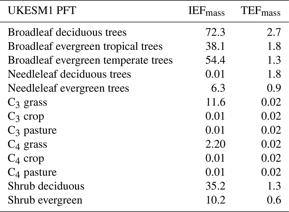
iBVOC was first implemented with the original five-PFT set-up in UKESM1 which divides vegetated regions into the categories of broadleaf trees, needleleaf trees, C₃ grass, C₄ grass and shrubs. IEF_mass values (Table 1) and the standard conditions were taken from Guenther et al. (1995).

Table 1 IEF in the five-PFT set-up.

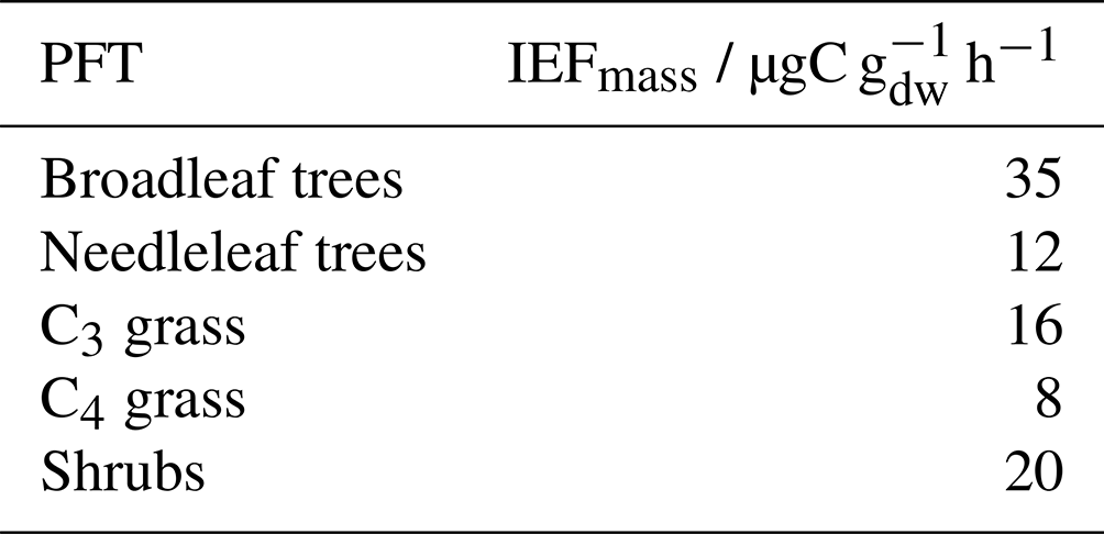
When running JULES stand-alone over the period 1990–1999, these IEF_mass values yielded simulated total isoprene emissions of 535 TgC yr⁻¹ (606 Tg_isoprene yr⁻¹), with 9 % coming from C₄ grass (Pacifico et al., 2011).

To improve land surface modelling, configurations of JULES with 9 and 13 PFTs were developed with the 13-PFT approach, the current standard in UKESM1 (Table 2) and the configuration used for UKESM1's contributions to CMIP6 (Sellar et al., 2020). Going from the 5-PFT configuration to the 13-PFT configuration, EF_mass values were assigned partly from those used in the 5-PFT configuration (e.g. the 13-PFT broadleaf deciduous tree category has the same IEF_mass as the 5-PFT broadleaf tree category) and partly from the Organizing Carbon and Hydrology in Dynamic Ecosystem (ORCHIDEE) vegetation scheme (Lathière et al., 2006). Unlike the 5-PFT configuration, the 13-PFT configuration does not appear to have been separately validated against observations or other model estimates, and furthermore, the IEF_mass of C₄ grass was increased from 8 to 24 µgC g${}_{\mathrm{dw}}^{-\mathrm{1}}$ h⁻¹ (Table 2).

Table 2 IEF_mass (µgC g${}_{\mathrm{dw}}^{-\mathrm{1}}$ h⁻¹) in the 13-PFT set-up of UKESM1.

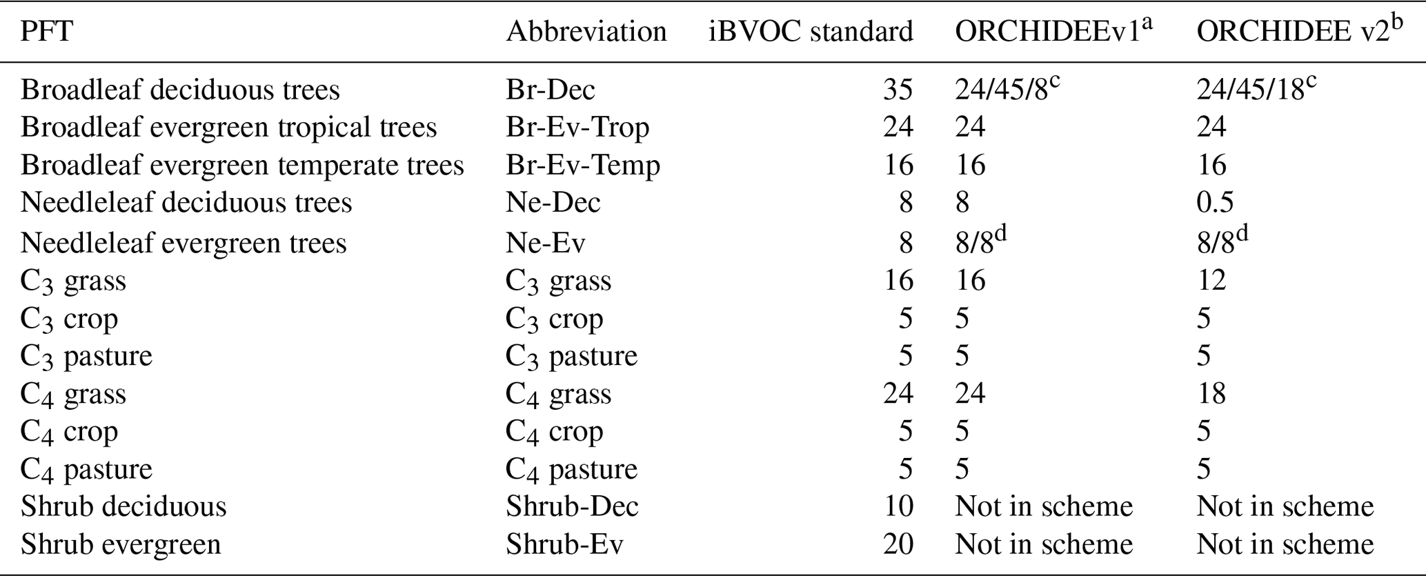
^a Lathière et al. (2006), ^b Messina et al. (2016), ^c tropical/temperate/boreal, area-weighted mean, ^d temperate/boreal.

In the context of this study, the limitation with using ORCHIDEE-derived EF_mass values for the 13-PFT configuration in UKESM1 is that the ORCHIDEE scheme does not simulate shrubs as a separate PFT. Rather, the IEFs from shrubs are incorporated into the IEF for C₃ and C₄ grass ORCHIDEE PFTs. This means that the C₃ and C₄ grass PFTs in ORCHIDEE are not equivalent to those in UKESM1 and should not be used to provide the IEF values.

Lathière et al. (2006) noted that ORCHIDEE considers high IEF values for grasses and also acknowledged the high degree of uncertainty in this area, as several other studies have found low emissions of isoprene from grasses and that a change to these values would lead to different regional distributions of emissions, a topic explored in Sect. 4.

In the updated version of ORCHIDEE, Messina et al. (2016) also note the inclusion of shrubs in the EF values for the grass PFTs in ORCHIDEE, and it remains unclear whether the ORCHIDEE values for C₃ and C₄ grass are composed totally or only partially of the EF_mass from shrubs. Nevertheless, as UKESM1 simulates deciduous and evergreen shrubs as separate PFTs with their own emission factors, including the IEF_mass of shrubs in those for grasses is not correct.

Furthermore, as shrubs are relatively strong isoprene emitters (e.g. Lathière et al., 2006; Guenther et al., 2012) and C₄ grasses are not (e.g. Guenther et al., 2012; Loreto and Fineschi, 2015), this approach artificially increases the isoprene production potential from the UKESM1 C₄ grass PFTs. This is exacerbated by the fact that large swathes of C₄ grassland are in warm regions (e.g. sub-Saharan Africa and eastern Brazil), further increasing isoprene production given its strong temperature dependence (for example, isoprene emissions are 35 % higher in iBVOC at 28 ^∘C than 25 ^∘C). Shrubs by contrast are typically found in higher-latitude regions where the lower temperatures lead to lower isoprene emissions, despite the relatively high IEF.

2.2 MEGAN v2.1 in CESM2

The Community Earth System Model version 2 (CESM2) is another Earth system model which includes atmospheric, land, ocean and sea ice models that can be run in stand-alone or coupled configurations (Danabasoglu et al., 2020). The land model component is the Community Land Model version 5 (CLM5) (Lawrence et al., 2019), which also simulates BVOC emissions based on prevailing atmospheric conditions and land surface cover using MEGAN v2.1. The development of MEGAN is described in Guenther et al. (1995, 2006, 2012). Like iBVOC, MEGAN v2.1 includes parameterisations for dependencies on temperature, CO₂ and PAR while also describing the impact of leaf age and soil moisture. A full description of the parameterisations is given in Guenther et al. (2012). CLM5 has 16 types of natural vegetation (including bare ground) and eight active crops. Similarly to JULES, vegetation and crops are represented by PFTs, each having specific ecophysiological, phenological and biogeochemical parameters (Lawrence et al., 2019). MEGAN v2.1 combines these parameterisations with PFT-specific emission factors (which for MEGAN have units of µg m${}_{\mathrm{surface}}^{-\mathrm{2}}$ h⁻¹) to calculate BVOC emissions for a range of BVOCs. Furthermore, unlike ORCHIDEE, MEGAN v2.1 considers grasses and shrubs separately, with emission factors for each. This means that the MEGAN EFs for C₃ and C₄ grasses are more suitable as a starting point for calculating EF values for iBVOC.

2.3 Calculation of EF_mass from MEGAN for iBVOC

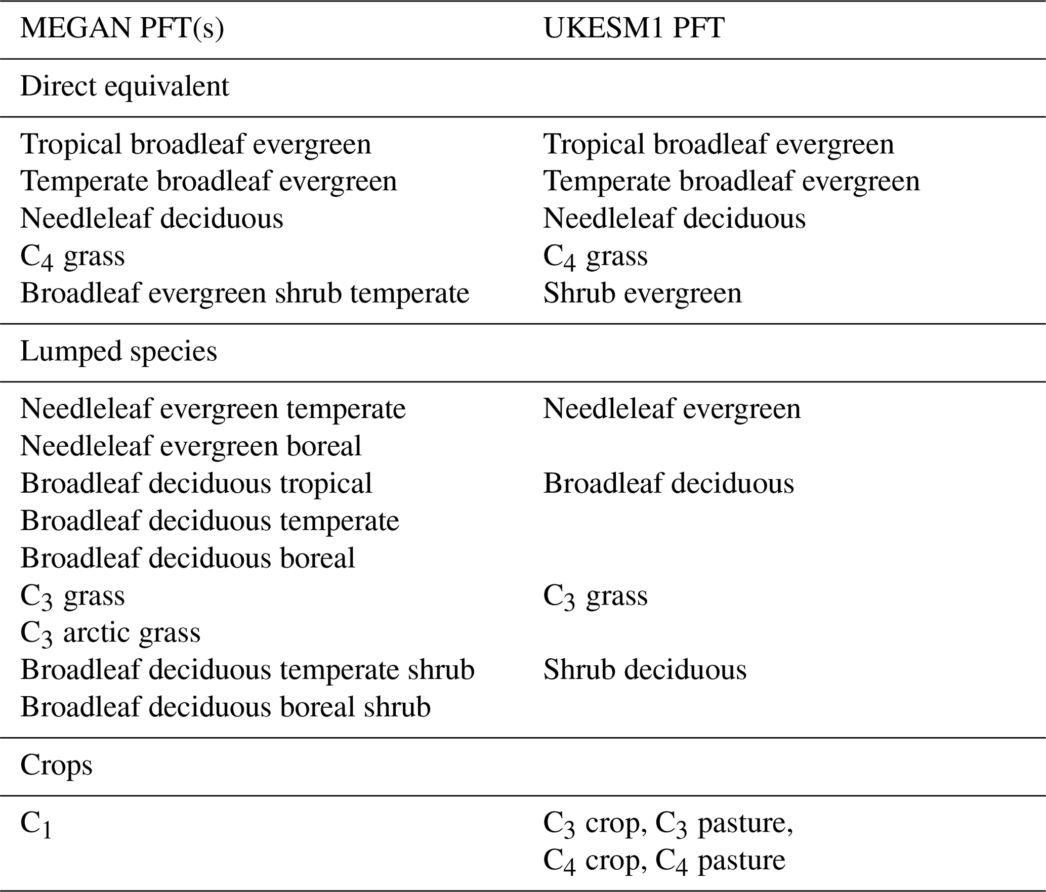
In this study, we use the MEGAN v2.1 EF (Table 3 of Guenther et al., 2012) as it offers an alternative source of EFs. We note that the same EFs for isoprene are used in the more recently released version MEGAN v3.0 (e.g. Zhang et al., 2021). MEGAN v2.1 in CESM2 considers 15 PFTs (excluding bare soil), so we had to lump certain PFTs during the conversion to IEF for iBVOC to match the 13-PFT classification in JULES. Table 3 shows the MEGAN v2.1 (CESM2) PFTs and the corresponding equivalents in iBVOC (UKESM1). Only seven PFTs in MEGAN v2.1 have a direct equivalent in UKESM1, allowing direct calculation of the EF_mass; the other eight PFTs were lumped into groups and the Crop 1 PFT in MEGAN v2.1 was used for the C₃ and C₄ crop and pasture PFTs in UKESM1.

Table 3 MEGAN PFTs and corresponding UKESM1 PFTs.

EFs in MEGAN are given in units of mass of species per unit area of land surface per unit time (e.g. µg_isoprene m⁻² h⁻¹), as opposed to µgC g${}_{\mathrm{dw}}^{-\mathrm{1}}$ h⁻¹ used in UKESM1 and ORCHIDEE, and are denoted hereafter as IEF_area. Therefore, a conversion must be applied to make these values comparable to the EFs used by iBVOC and ORCHIDEE, which are denoted as IEF_mass.

To convert EF_area to EF_mass, we adapt Eq. (5) of Messina et al. (2016) to yield Eq. (1).

$$\begin{array}{}\text{(1)}& {\mathrm{EF}}_{\mathrm{mass}}={\mathrm{IEF}}_{\mathrm{area}}\times {\displaystyle \frac{\mathrm{1}}{{\mathrm{LAI}}_{\mathrm{ref}}}}\times {\displaystyle \frac{\mathrm{1}}{\mathrm{SLW}}}\times {\displaystyle \frac{m_{\mathrm{Carbon}}}{m_{\mathrm{species}}}}\times {\displaystyle \frac{\mathrm{1}}{{\mathrm{C}}_{\mathrm{CE}}}},\end{array}$$

where LAI_ref is the reference leaf area index used by MEGAN v2.1 (5 m${}_{\mathrm{leaf}}^{\mathrm{2}}$ m${}_{\mathrm{surface}}^{-\mathrm{2}}$), SLW is the specific leaf weight (g_dw m${}_{\mathrm{surface}}^{-\mathrm{2}}$), the factor $\frac{m_{\mathrm{Carbon}}}{m_{\mathrm{Species}}}$ accounts for the fact that MEGAN v2.1 considers the mass flux of a given species and iBVOC and ORCHIDEE the mass flux of carbon, and C_CE is the MEGAN canopy environment coefficient (0.57).

Equation (1) is valid for emissions which are entirely dependent on PAR, as is the case for isoprene in MEGAN v2.1. Emissions of monoterpenes have a light-dependent fraction (LDF) and a light-independent fraction (LIDF = 1 − LDF). In this case, Eq. (1) needs to be modified to give Eq. (2).

$$\begin{array}{}\text{(2)}& \begin{array}{rl}{\mathrm{EF}}_{\mathrm{mass}}& ={\mathrm{IEF}}_{\mathrm{area}}\times {\displaystyle \frac{\mathrm{1}}{{\mathrm{LAI}}_{\mathrm{ref}}}}\times {\displaystyle \frac{\mathrm{1}}{\mathrm{SLW}}}\times {\displaystyle \frac{m_{\mathrm{Carbon}}}{m_{\mathrm{species}}}}\\ & \times \left({\displaystyle \frac{\mathrm{LDF}}{{\mathrm{C}}_{\mathrm{CE}}}}+\left(\mathrm{1}-\mathrm{LDF}\right)\right)\end{array}\end{array}$$

The LDF varies between species, and we used the values given in Table 4 of Guenther et al. (2012).

There are three main areas of uncertainty in the conversion: the lumping of PFTs, the choice of SLW values and, for terpene emissions, the choice of input TEF_area values.

2.3.1 PFT lumping

We lump the MEGAN PFTs (Table 3) by calculating the mean EF value weighted by the area of each PFT. For example, the EF for the UKESM1 needleleaf evergreen PFT is calculated as the mean of the MEGAN EF for needleleaf evergreen temperate and needleleaf evergreen boreal weighted by the total areas of these two species. We use the year 2000 LULC specified in Table 3 of Guenther et al. (2012) for this lumping. The resulting EF_area value is then used in Eq. (1) to calculate EF_mass.

This approach necessarily introduces a dependency on the LULC assumption employed because different LULC datasets (i.e. CESM, ORCHDIEE, UKESM1) report different total areas for each PFT. We also acknowledge that LULC cover is likely to be different in past or future LULC scenarios, affecting the validity of the weighting to some degree. However, this impact is expected to be small and would also occur if the ORCHIDEE scheme were used since it also has a greater speciation of PFTs than UKESM1.

2.3.2 SLW values

One source of uncertainty in the EF_mass $/$ EF_area conversion is the PFT-specific values of SLW. MEGAN v2.1 does not use SLW (personal communication with Alex Guenther, 6 April 2022), and we consider three other datasets of SLW from CLM5, ORCHIDEE and UKESM1.

CLM5 uses specific leaf area (SLA; m² gC⁻¹) at the canopy top for photosynthesis calculations (Ali et al., 2016), and we consider the inverse for SLW and apply a scaling of 2 to convert the mass of carbon to dry leaf mass.

The ORCHIDEE BVOC scheme also reports SLA (m${}_{\mathrm{leaf}}^{\mathrm{2}}$ gC⁻¹) (SLW; gC m${}_{\mathrm{leaf}}^{-\mathrm{2}}$) (Table S1 in the Supplement). Similar to the CLM5 SLW, we apply a scaling of 2 to convert mass of carbon to dry leaf mass. For UKESM1, we use the reported values of SLW (termed leaf mass area or lma; g_dw m⁻²) for the 13 PFTs.

Figure 1 shows the three SLW datasets with the CLM5 and ORCHIDEE values lumped into UKESM1 PFTs. We find reasonable agreement, particularly between UKESM1 and CLM5 for the major emitting species.

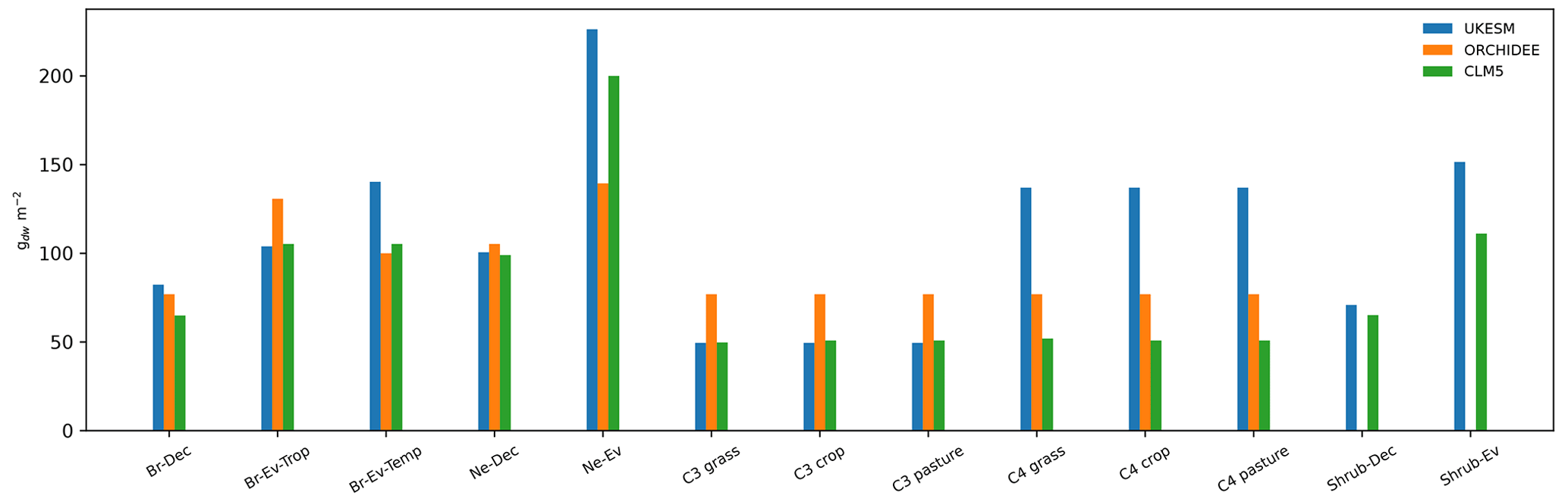
Figure 1 SLW values for UKESM1 PFTs from the UKESM1, ORCHIDEE and CLM5 datasets. ORCHIDEE does not consider shrubs to be separate PFTs, so there are no corresponding SLW values.

To explore the uncertainty arising from the variation in SLW, we calculate EF_mass using the UKESM1, CLM5 and ORCHIDEE SLW datasets. When calculating the EF_mass using the CLM5 and ORCHIDEE SLW values, we first calculate the EF_mass for the scheme-specific PFTs (i.e. for the 15 PFTs in MEGAN) and then perform the lumping (Table 3). By contrast, when calculating the EF_mass using the SLW which correspond to UKESM's 13 PFTs, the EF_area from MEGAN v2.1 must be lumped first before being converted to EF_mass.

2.3.3 Temperature scaling

It is also necessary to consider the fact that the “standard conditions” differ between MEGAN v2.1, ORCHIDEE and iBVOC.

The temperature factor in MEGAN v2.1, γ_T, uses a parameterisation which considers the standard conditions for leaf temperature (T_s=297 K) and the average leaf temperature of the past 24 (T₂₄) and 240 (T₂₄₀) h (Eqs. 8–10; Guenther et al., 2012). ORCHIDEE and UKESM1 assume that leaf and air temperature are the same and use standard conditions of 303.15 K (30 ^∘C). Therefore, it is necessary to scale the IEF_mass in Eqs. (1) and (2) to account for difference in standard temperature.

For isoprene emissions, iBVOC applies a temperature dependence (Eq. 3) (Pacifico et al., 2011) as

$$\begin{array}{}\text{(3)}& T_{\mathrm{isop}}=min[e^{\mathrm{0.1}\left(T-\mathrm{303.15}\right)};\mathrm{2.3}].\end{array}$$

In this work, we apply a temperature scaling T_{isop_scale} (Eq. 4) using this temperature dependence to account for the difference in standard conditions.

$$\begin{array}{}\text{(4)}& T_{\mathrm{isop}\mathrm{\_}\mathrm{scale}}={\displaystyle \frac{T_{\mathrm{isop}\mathrm{@}\mathrm{303.15}\mathrm{K}}}{T_{\mathrm{isop}\mathrm{@}\mathrm{297}\mathrm{K}}}}={\displaystyle \frac{e^{\mathrm{0.1}(\mathrm{303.15}-\mathrm{303.15})}}{e^{\mathrm{0.1}(\mathrm{297}-\mathrm{303.15})}}}=\mathrm{1.85}\end{array}$$

iBVOC also applies a temperature dependence to terpene emissions (T_terp) in the 13-PFT set-up for all PFTs, except for broadleaf deciduous trees, whose parameterisation we describe later (Pacifico et al., 2011) (Eq. 5).

$$\begin{array}{}\text{(5)}& T_{\mathrm{terp}}=e^{\mathrm{0.09}\left(T-\mathrm{303.15}\right)}\end{array}$$

Following the same approach as for isoprene emissions, we apply a scaling factor T_{terp_scale} (Eq. 6).

$$\begin{array}{}\text{(6)}& T_{\mathrm{terp}\mathrm{\_}\mathrm{scale}}={\displaystyle \frac{T_{\mathrm{terp}\mathrm{@}\mathrm{303.15}\mathrm{K}}}{T_{\mathrm{terp}\mathrm{@}\mathrm{297}\mathrm{K}}}}={\displaystyle \frac{e^{\mathrm{0.09}\left(\mathrm{303.15}-\mathrm{303.15}\right)}}{e^{\mathrm{0.09}\left(\mathrm{297}-\mathrm{303.15}\right)}}}=\mathrm{1.74}\end{array}$$

In iBVOC, terpene emissions for broadleaf deciduous trees are assumed to have a PAR-independent component and a PAR-dependent component (terpene emissions for all other PFTs are assumed to be entirely PAR-independent). In a similar approach to MEGAN v2.1 (Sect. 2.2; Guenther et al., 2012), the PAR-independent component uses the terpene temperature dependence (T_terp; Eq. 5), while the PAR-dependent component uses the isoprene temperature dependence (T_isop; Eq. 3) along with an additional term representing photosynthesis. These components have a 50:50 weighting, and we therefore use an average of T_{isop_scale} and T_{terp_scale} for the temperature scaling, T_{terp_BrDe_scale}, for this PFT (Eq. 7).

$$\begin{array}{}\text{(7)}& T_{\mathrm{terp}\mathrm{\_}\mathrm{BrDe}\mathrm{\_}\mathrm{scale}}=\mathrm{0.5}{T}_{\mathrm{terp}\mathrm{\_}\mathrm{scale}}+\mathrm{0.5}{T}_{\text{isop\_scale}}=\mathrm{1.79}\end{array}$$

It is important to note that MEGAN v2.1 uses a more complicated temperature dependence which considers average leaf temperatures over the previous 24 and 240 h. MEGAN v2.1 and iBVOC also differ in their simulation of CO₂ inhibition (which is PFT-specific for iBVOC but not in MEGAN) and photosynthesis. Both models simulate reductions in isoprene emissions with CO₂. The CO₂ inhibition parameterisation in iBVOC follows that of Arneth et al. (2007), considering the ratio of the plant's internal CO₂ concentration to a PFT-specific reference value, while MEGAN uses the parameterisation of Heald et al. (2007), which is not PFT-specific. Cao et al. (2021) found the CO₂ inhibition in UKESM (using iBVOC) to be almost twice that of CESM (using MEGAN) when considering isoprene emissions in the late 21st century. MEGAN parameterises the effect of photosynthesis with a scaling term composed of a LDF and LIDF (1 − LDF), with the former a function of the photosynthetic photon flux density averaged over a 24 h period for both shaded and unshaded leaves (Sect. 2.2, Guenther et al., 2012). By contrast, iBVOC describes the impact of photosynthesis from the perspective of electron transport, following Arneth et al. (2007) as described in Sect. 2.2 of Pacifico et al. (2011). MEGAN v2.1 also features a parameterisation to account for the influence of leaf age on emissions, while iBVOC does not. Accounting for these parameterisation differences is very complicated and has not been done in this conversion.

2.3.4 EF for terpene emissions

For terpenes a further factor in the conversion must be considered. Unlike isoprene, where the tracer in UKCA corresponds directly to the molecule isoprene, the one or two terpene tracers in UKCA actually represent a wide range of monoterpene species.

The Strat-Trop (ST) chemistry scheme (Archibald et al., 2020), the standard in UKESM1, considers a single tracer, Monoterp (MT), whose initial oxidation reactions with OH, O₃ and NO₃ have the rate constants of the most widely emitted monoterpene, α-pinene. The alternative mechanism, CRI-Strat 2 (CS2) (Weber et al., 2021), considers separate α-pinene and β-pinene tracers which have different rate constants. When using the ST mechanism, terpene emissions calculated by iBVOC are mapped directly to MT emissions considered by UKCA, while in CS2, terpene emissions are split into a 2:1 ratio for α-pinene and β-pinene, representing the approximate global emission ratio of these species (Sindelarova et al., 2014).

MEGAN v2.1 provides separate PFT-specific EF_area for α-pinene, β-pinene, myrcene, sabinene, limonene, 3-carene and t-β-ocimene and for an “other monoterpenes” category. For the major emitting PFTs, the EF_area of α-pinene are ∼ 60 % higher than those of β-pinene and 2 to 3 times higher than those of the other specific monoterpenes (e.g. myrcene) and the “other monoterpenes” category. Since the emissions of MT in ST and α-pinene and β-pinene in CS2 represent all monoterpenes, a choice must be made regarding how to combine these EF_area.

In this analysis, we consider three options – using only the α-pinene EF_area, using the α-pinene and β-pinene EF_area in a 2:1 weighted mean (representing the ratio of these species in Sindelarova et al., 2014) or using the α-pinene, β-pinene and “other monoterpenes” EF_area in a mean weighted by the total emission estimates in Sindelarova et al. (2014), namely $\mathrm{32}:\mathrm{16.7}:\mathrm{46.3}$. Sindelarova et al. (2014) do not speciate monoterpenes beyond α-pinene, β-pinene and total monoterpenes, so inclusion of the EF_area of the other species like myrcene was not considered here.

2.3.5 EF_mass values

Figure 2 shows the PFT-specific EF_mass values for isoprene (IEF_mass) and terpene (TEF_mass) calculated using the SLW datasets and, in the case of TEF_mass, the three different combinations of the monoterpene EF from MEGAN v2.1. We also show the current IEF_mass and TEF_mass used by UKESM1.

Unsurprisingly, the new approach yields substantially lower EF_mass values for C₄ grass, crops and pasture compared to the UKESM1 default. The IEF_mass of needleleaf deciduous trees decreases to almost zero (its IEF_area has the joint lowest value in MEGAN v2.1), while the IEF_mass and TEF_mass of all broadleaf trees increase.

Figure 2 Default and new (a) IEF_mass and (b) TEF_mass for UKESM1 PFTs.

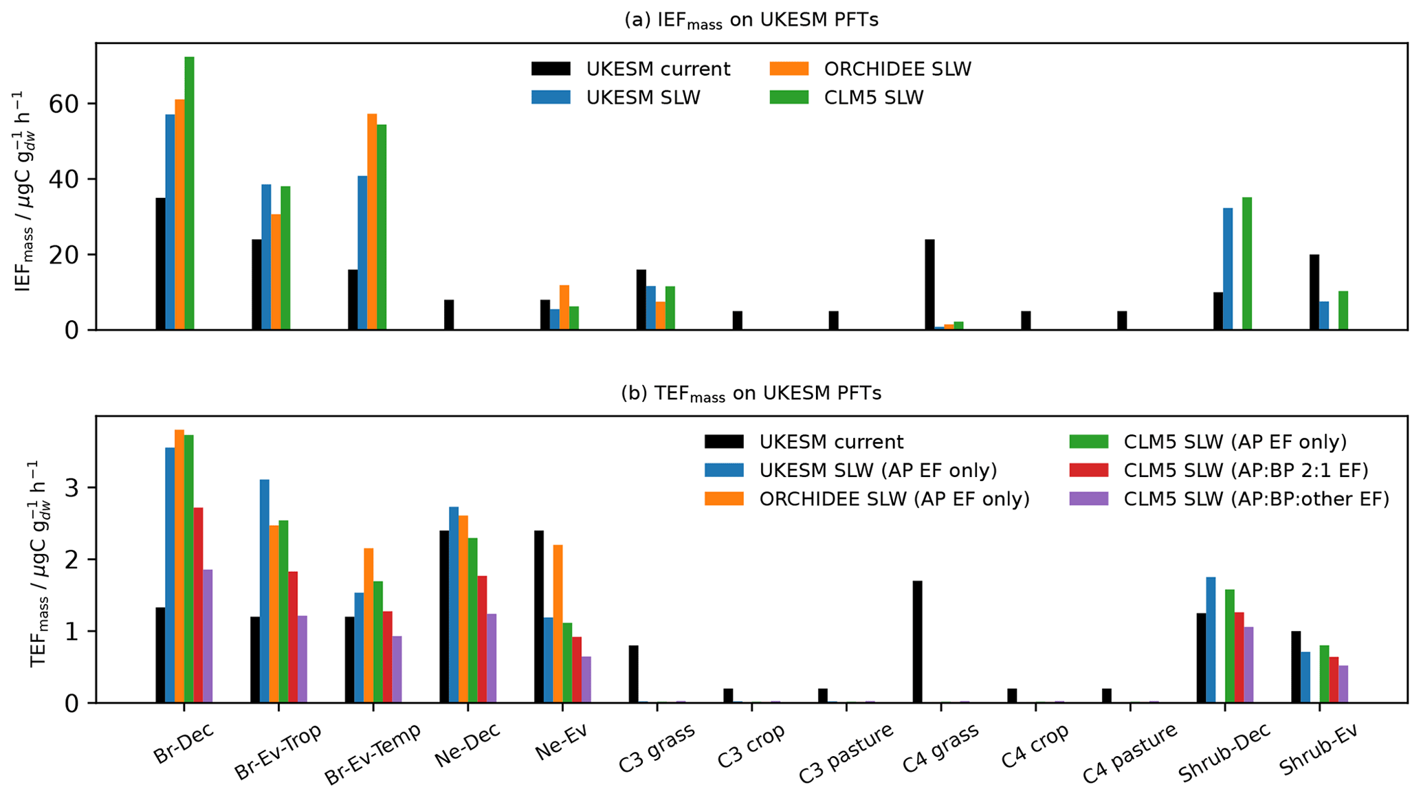
The variation in EF_mass from uncertainty in SLW is particularly notable for the broadleaf deciduous and broadleaf evergreen temperate PFTs but smaller for the broadleaf evergreen tropical PFT, the single largest emitter of isoprene. The impact of this uncertainty on isoprene emissions is explored by comparing emissions from UKESM1 simulations using the IEF_mass calculated using UKESM1 SLW and CLM5 SLW (Table 4; Evaluation). This was not done for terpene emissions since the choice of EF_area is likely to be a much larger source of uncertainty.

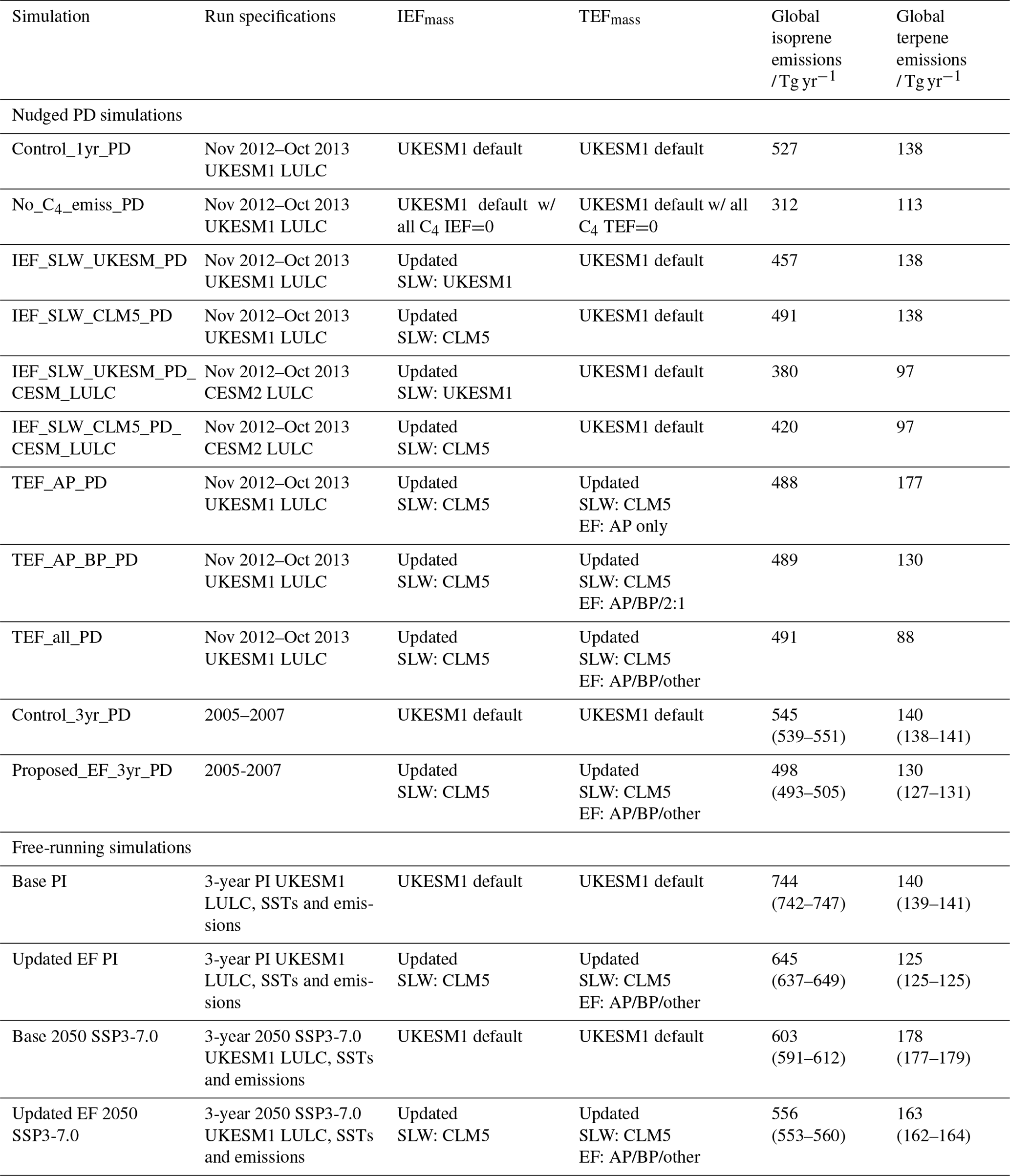
Table 4 Evaluation simulations with UKESM1. Reported are the average for 1-year simulations and the average and range of annual means (in parentheses) for multi-year simulations. The UKESM1.0 simulations used UM version 12.0.

3 Evaluation simulations

To assess the impact of changing the EF_mass values, we performed a range of simulations in UKESM1 with varying IEF_mass and TEF_mass values and two accompanying simulations in CESM2 for comparison purposes. We also evaluated the resulting simulated isoprene columns against satellite observations from the Cross-track Infrared Sounder (CrIS) and ground observations. Tables 4 and 5 summarise the simulations performed for this evaluation.

Table 5 Evaluation atmosphere-only simulations with UKESM1 and CESM performed to investigate responses to LULC change with different EFs. The UKESM1.0 simulations used UM version 12.0. All the simulations used SSTs from SSP3-7.0 at 2050 and WMGHGs and anthropogenic and biomass burning emissions from 2010.

3.1 UKESM1 simulations

All UKESM1 simulations used the atmosphere-only configuration of UKESM1 run at a horizontal resolution of 1.25^∘ × 1.875^∘ with 85 vertical levels up to 85 km (Walters et al., 2019) and the GLOMAP-mode aerosol scheme, which simulates sulfate, sea salt, BC and organic matter but does not simulate currently nitrate aerosol (Mulcahy et al., 2020). Mineral dust is simulated using the bin scheme of Woodward (2001). UKESM1 has the capability to perform simulations using specified dynamics, also called “nudging”, where certain offline meteorological fields from the ERA-Interim reanalysis (temperature and horizontal winds) are input (Dee et al., 2011) and free running with online computed meteorology.

Our evaluation has three sections. Firstly, we perform PD simulations nudged to atmospheric reanalyses to compare the model simulations with different EF_mass values to observational data (Table 4). Secondly, we perform free-running simulations using conditions from the pre-industrial (PI) and Shared Socioeconomic Pathway SSP3-7.0, which represents a “regional rivalry” scenario at 2050 (O'Neill et al., 2016) to assess the effect these different EF_mass values would have in these two periods (Table 4). Finally, we perform free-running simulations using PD conditions but with LULC from either the PD or specific future LULC scenario featuring wide-scale reforestation/afforestation to assess the impact these EF_mass values would have on the response of mass tree planting (Table 5). Runs used the CS2 chemical mechanism (Jenkin et al., 2019; Weber et al., 2021), version 12.0 of the Unified Model (UM) and vn5. of JULES.

Nine 1-year PD simulations were performed for November 2012–October 2013, as this period covers 4 months for which there exist satellite CrIS observations of global isoprene columns (January, April, July and October 2013; Wells et al., 2020). Six runs were performed to evaluate plausible EF_mass approaches by comparison of the resulting total global emissions to estimates from other sources and, for isoprene, comparison of simulated column values against measured column values. No_C4_emiss_PD was run to isolate the fraction of emissions from C₄ PFTs (see Sect. 4). Finally, two 3-year nudged PD simulations were run with UKESM1 default EF_mass and the proposed new EF_mass to ensure the trends established in the 1-year runs were not simply caused by the prevailing meteorology and persisted over a longer period. We also performed two UKESM1 simulations using LULC taken from a PD CESM2 simulation (with PFTs lumped as described in Sect. 2) to assess the influence of the underlying simulated LULC on emissions. These simulations, IEF_SLW_UKESM_PD_CESM_LULC and IEF_SLW_CLM5_PD_CESM_LULC (Table 4), used the same IEF values as IEF_SLW_UKESM_PD and IEF_SLW_CLM5_PD respectively.

Nudging of temperature and horizontal wind was used to prevent diverging meteorology affecting BVOC emissions and to replicate as closely as possible the atmospheric conditions experienced when the observations were recorded. Thus, nudging, along with the use of observed sea surface temperature (SST) fields, means that, as far as possible, the changes in EF_mass will be the only drivers of emission changes and allows for a more faithful comparison to observational data. Nudging only occurred above ∼ 1200 m in altitude, and thus most of the planetary boundary layer was not nudged.

The 1-year PD nudged runs used time series of anthropogenic and biomass burning emissions to keep the simulated conditions close to those when the observations were recorded. The 3-year nudged PD runs used 2014 time-slice anthropogenic and biomass burning emissions. All these simulations used prescribed LULC from a UKESM1 historical ensemble member performed for CMIP6 (Sellar et al., 2020).

The four free-running simulations performed to investigate how the EF_mass changes would affect simulated emissions in the PI and in 2050 under conditions used prescribed LULC from the UKESM1 piControl and SSP3-7.0 runs performed for CMIP6 (Sellar et al., 2019) and time-slice emissions from 1850 and SSP3-7.0 2050 respectively (Table 4).

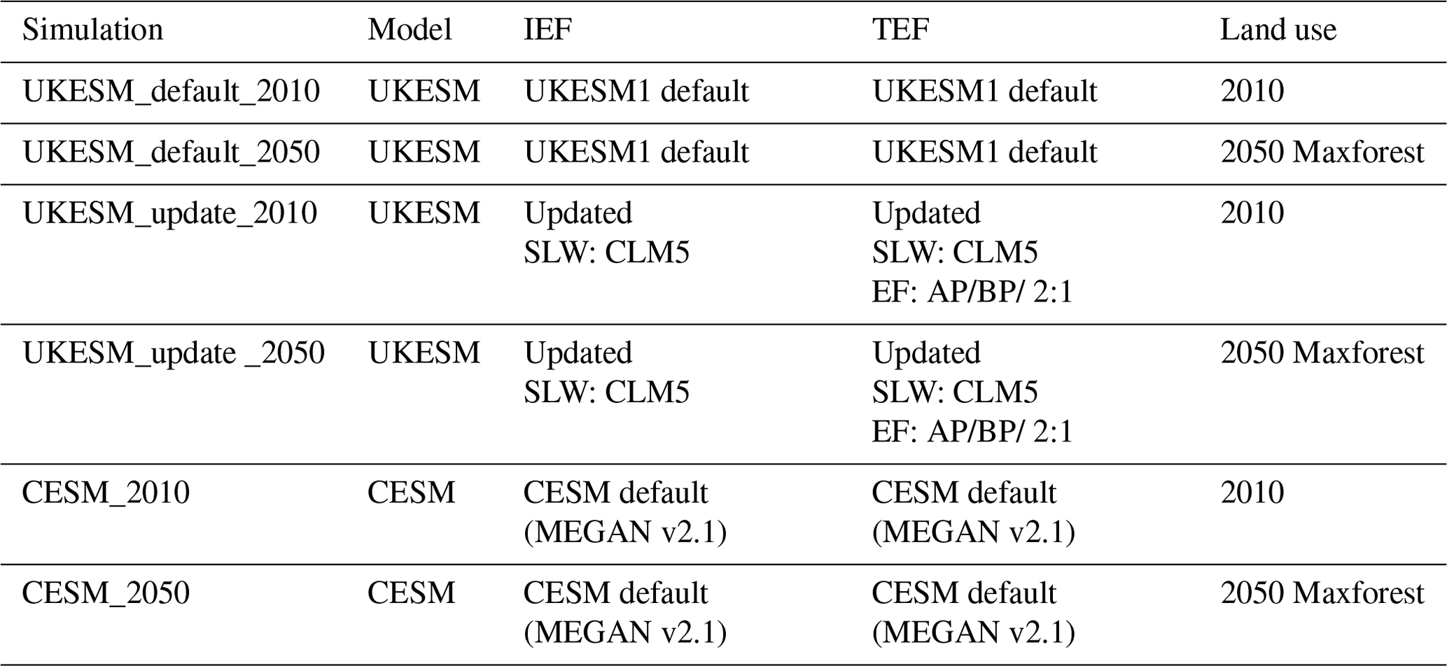
We also explored how the change to EF_mass would affect the response to a specific LULC change with a further set of simulations, which used two time periods from a specific land use scenario featuring wide-scale afforestation and reforestation (“MaxForest”). The Maxforest scenario features a very high degree of reforestation and afforestation over the course of the 21st century and was developed to assess the impact of such LULC with regards to carbon sequestration, among other factors. The scenario gradually expands existing forested regions with suitable tree species and also avoids encroachment on cropland, pastures and urban regions. It can thus be considered a scenario representing a near-maximum plausible level of reforestation/afforestation. The Maxforest scenario was originally developed for CLM5 (Lawrence et al., 2019), and we adapted it for UKESM1 using the same lumping of PFTs as discussed in Sect. 2.3.1. We performed simulations with the default and new EF_mass values with LULC from the start of the MaxForest scenario at 2010 (no increase in tree cover) and at 2050, when extensive reforestation was well underway. All these simulations used PD anthropogenic and biomass burning emissions and GHG concentrations, but BVOC emissions were allowed to respond to LULC change. We compare the change in isoprene and terpene emissions between 2010 and 2050 Maxforest land use when the default EF_mass values were used to when the new EF_mass values were used. We also performed the same experiments in CESM2 (Sect. 3.2) and compare the change in BVOC emissions between 2010 and 2050 Maxforest land use to the UKESM simulations.

In all the runs, CO₂ was not emitted but was set to a constant field appropriate for the PI, PD and 2050 under SSP3-7.0 conditions, while the other well-mixed greenhouse gases (WMGHGs) CH₄, CFCs and N₂O were prescribed with constant lower-boundary conditions (Archibald et al., 2020) appropriate for the PI, PD and 2050 under SSP3-7.0 conditions.

Fields for SSTs, sea ice (SI) and ocean biogeochemistry (DMS – dimethyl sulfide – and chlorophyll) were prescribed for all the runs. The nudged PD runs used observed SSTs and SI and ocean biochemistry from a UKESM1 historical ensemble member. The free-running PI runs used a 30-year mean from the UKESM1 piControl for SSTs, SI and ocean biogeochemistry. The SSP3-7.0 2050 runs used 2050 ocean biogeochemistry and 2045–2055 mean SSTs and SI, all taken from one of the UKESM1 SSP3-7.0 ensemble members.

The free-running Maxforest simulations (Table 5) used 2050 ocean biogeochemistry, 2045–2055 mean SSTs and SI and PD anthropogenic emissions and prescribed concentrations of WMGHGs. The same SSTs and WMGHG concentrations were applied to ensure differences in BVOC emissions were due to LULC only.

All UKESM1 runs used oceanic emissions of CO, C₂H₄, C₂H₆, C₃H₆ and C₃H₈ from the POET 1990 dataset (Olivier et al., 2003), and all biogenic emissions except isoprene and monoterpenes were based on 2001–2010 climatologies from the MEGAN-MACC (Monitoring Atmospheric Composition and Climate) dataset (Sindelarova et al., 2014) calculated by the MEGAN v2.1 model (Guenther et al., 2012) under the MACC project. Emissions of isoprene and monoterpenes (split into a 2:1 ratio between α-pinene and β-pinene) were calculated interactively using iBVOC. Anthropogenic and biomass burning emission data for CMIP6 are from the Community Emissions Data System (CEDS), as described by Hoesly et al. (2018).

3.2 CESM simulations

The CESM simulations used version 2.2.0 (Danabasoglu et al., 2020) at a 0.9^∘ × 1.25^∘ horizontal resolution. For the atmospheric component, we employ CAM-chem version 6 (hereinafter CAM6-chem), with a full tropospheric O₃–NO_x–CO–VOC–aerosol chemistry based on an updated tropospheric chemistry mechanism (MOZART-TS1) (Emmons et al., 2020) with the Modal Aerosol Model with 4 modes (MAM4) (Liu et al., 2016). CAM6-chem has 32 vertical layers and a model top of ∼ 45 km and is coupled to CLM5, which provides BVOCs with the MEGAN v2.1 scheme and handles dry deposition. Our simulations used specified sea surface temperatures and thermodynamic sea ice.

For the two CESM simulations, anthropogenic and biomass burning emissions of reactive gases and aerosols were fixed to a 2010 climatology (2006–2014 average) using data from Hoesly et al. (2018). WMGHGs were incorporated as fixed lateral boundary conditions rather than as emissions from the surface and were also fixed to 2010 values (2006–2014 average) using standard concentration data from CMIP6 (Meinshausen et al., 2017).

For LULC, we performed the same free-running PD and 2050 LULC simulations as in UKESM1 (Table 5) to allow comparison of the BVOC emission responses to the LULC change in UKESM1 and CESM. As with UKESM1, the CESM simulations were atmosphere-only and used PD anthropogenic emissions and prescribed WMGHG concentrations and 2045–2055 mean SSTs, with the only difference between the simulations being the LULC.

3.3 Observational data

Monthly mean isoprene columns derived using the space-borne CrIS technique (Wells et al., 2020) were used as the principal method of evaluation since it all allows the regional changes to be readily assessed. The CrIS is a longwave infrared Fourier transform spectrometer on board a satellite which can measure two isoprene IR absorption features. The absorption data collected by the spectrometer are then combined with an artificial neural network to calculate isoprene columns.

Surface isoprene emission measurements from regions with C₄ grass were also used to examine the impact of substantial reduction in C₄ grass IEF_mass. In lieu of observations from C₄-only regions (which are very sparse given the understanding that C₄ grasses are weak isoprene emitters), we use observations from savanna, which tends to comprise grasses, woody shrubs and a range of trees, including strong isoprene and monoterpene emitters (e.g. Table 3 of Otter et al., 2002), in varying proportions. We select savanna observations from sites specifically noted as being without dominant isoprene emitters (Central Africa Republic – Klinger et al., 1998; Nylsvley, South Africa – Guenther et al., 1996, and Otter et al., 2002). We note that these sites were likely to have grass species with very low isoprene emissions, below the instrument detection limits (e.g. Harley et al., 2003). Therefore, our compiled observations represent an upper bound for isoprene emissions from C₄ grass.

We also used monoterpene emission data measured at the SMEAR II site in Hyytiälä (https://smear.avaa.csc.fi, last access: 19 March 2023) to evaluate the change in terpene emissions.

4 Results

The impact of changing EF_mass values is assessed in terms of total isoprene and monoterpene emissions and, in the case of isoprene, against global isoprene column values. We also discuss the change in the contribution to total emissions from the different PFTs and the impact of the EF_mass changes on simulated emissions in the PI, at 2050 under SSP3-7.0, and the reforestation/afforestation LULC scenario.

4.1 Total global emissions

Table 4 presents the global isoprene and terpenes emissions in our simulations. For isoprene, all nudged PD simulations, except No_C₄_emiss_PD, yield total emissions within the range of previous estimates. Simulations using IEF_mass from UKESM1 SLW (“IEF_SLW_UKESM_PD”) and CLM5 SLW (“IEF_SLW_CLM5_PD”) yield emissions 13 % and 7 % lower than the UKESM1 control simulation (“Control_1yr_PD”) respectively.

When UKESM1 LULC was replaced with CESM2 LULC, isoprene emissions are 380 Tg yr⁻¹ (IEF_SLW_UKESM_PD_CESM_LULC) and 420 Tg yr⁻¹ (IEF_SLW_CLM5_PD EF). These values are lower than the 457 and 490 Tg yr⁻¹ simulated using the same IEF values and UKESM LULC, yet they are still well within the range of simulated emissions (310–680 Tg yr⁻¹) of Fig. 1 of Messina et al. (2016). This highlights the influence of uncertainty in LULC on BVOC emissions but, as iBVOC is chiefly for use with UKESM1, we will focus on the simulations using UKESM1 LULC.

For terpenes, when the TEF_mass is based solely on α-pinene (TEF_AP_PD), total emissions (177 Tg yr⁻¹) are higher than previously published results (Messina et al., 2016) and when the TEF_mass is derived from the weighted average of ratio of α-pinene, β-pinene and other monoterpenes” (TEF_all_PD), total emissions (88 Tg yr⁻¹) are at the lower end of estimates. However, when taking a 2:1 ratio of α-pinene and β-pinene TEF_area (TEF_AP_BP_PD), the resulting emissions (130 Tg yr⁻¹) are more in line with other estimates.

The clearest indication of the significant contribution C₄ PFTs make to BVOC emissions in the current UKESM1 set-up comes from the comparison of Control_1yr_PD and No_C₄_emiss_PD, where the EF_mass of all C₄ PFTs is zero, simulations. This reveals that C₄ PFTs contribute about 40 % (18 %) to total isoprene (terpene) emissions in the current UKESM1 set-up, far higher than the 1 % (0.3 %) estimated by Guenther et al. (2012), 9 % for isoprene from the original 5-PFT version of iBVOC (Pacifico et al., 2011) and 1 %–2 % for isoprene estimated by Pfister et al. (2008). As previously discussed, this substantial contribution from C₄ grasses is also in stark contrast to other studies, which highlight very low emissions of isoprene from C₄ grasses (e.g. Loreto and Fineschi, 2015). Overall, this suggests that while the current UKESM1 approach may produce a reasonable value for total isoprene and terpene emissions, these are derived using unrealistic EF for C₄ grasses.

With the updated EF_mass, the C₄ grass PFT contributes 1 %–3 % of total isoprene emissions (based on the chosen SLW) and 0.2 %–0.7 % of total terpene emissions (based on the choice of EF_area), bringing UKESM1 into line with other estimates.

The decreases in C₄ PFT EF_mass and increases in the EF_mass of the broadleaf evergreen tropical tree PFT lead to the contribution to total isoprene emissions from broadleaf evergreen tropical trees increasing from 45 % to 75 % (50 % to 80 % for terpenes). This contribution is greater than the 46 % estimated by MEGAN v2.1 (Guenther et al., 2012). However, the area of this PFT in UKESM1 is 67 % greater than CLM4 (26.0 vs. 15.6×10⁶ km²). (While this difference in area may seem large, the total areas of tropical trees in UKESM and CLM4 are much more similar if the area of CLM4's deciduous evergreen tropical tree PFT, for which there is no direct analogue in UKESM, is included.) On an emissions per unit area basis for the broadleaf evergreen tropical PFT, isoprene emissions in UKESM1 are within 5 % of that from Guenther et al. (2012), while terpene emissions are ∼ 25 % lower. This separately highlights the important issue of uncertainty in land use and land cover and the effect that it can have on model–model comparisons (e.g. in CMIP6) and model–observation comparisons.

Spatially, the new IEF_mass led to isoprene emission increases across Amazonia (albeit with a small reduction around Manaus) and the Congo and decreases north and south of the African rainforest, where the simulated C₄ grass PFT dominates (Fig. 3a). Terpene emissions increase over the tropics due to increases in the TEF_mass of tropical evergreen broadleaf trees, while they decrease at mid and high latitudes (Fig. 3b) from reductions in the TEF_mass of needleleaf evergreen and deciduous PFTs (Fig. 2b).

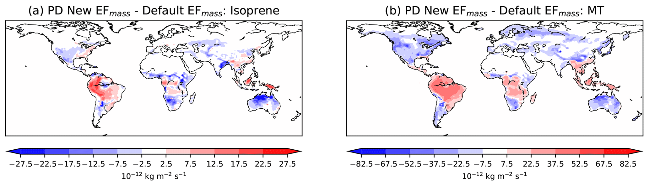
Figure 3 Three-year annual average change in (a) isoprene and (b) monoterpene (MT) emissions following the change in EF_mass values.

For the PI and future simulations with UKESM1 (Fig. S1), the new EF_mass values lead to reductions in total global isoprene (terpene) emissions of 13 % (11 %) and 8 % (8 %) in the PI and 2050 SSP3-7.0 scenarios respectively compared to the default EF_mass (Base PI). For both scenarios, isoprene emissions from C₄ PFTs decrease by ∼ 90 %, while emissions from broadleaf evergreen tropical trees increase by ∼ 50 %. This leads to emission increases over Amazonia and the Congo but decreases north and south of the Congo (Fig. S1a, c). Terpene emissions from C₄ PFTs drop to almost zero and decrease by ∼ 60 % from needleleaf evergreen trees while increasing by around 50 % from broadleaf evergreen tropical trees, driving a tropical emission increase and high-latitude emission decrease (Fig. S1b, d).

4.2 Isoprene column comparison

We compare the output from the PD simulations to the CrIS observed isoprene columns (Sect. 3.3) for January, April, July and October 2013 (Fig. 4). The use of nudging significantly reduces the difference in meteorology between the simulations and reality, greatly improving the comparability of modelled and observational data. However, the lowest 11 model levels (up to approx. 700–1000 m) are not nudged, so there will be some differences between the model simulation conditions and reality in the boundary layer, although this is tempered by the nudging applied to the higher levels.

For the 4 months considered, IEF_SLW_UKESM_PD and IEF_SLW_CLM5_PD yield lower total isoprene emissions than Control_1yr_PD but show generally slightly higher column biases in the same regions where the control run has a bias, chiefly in western Amazonia.

This bias exacerbation is slightly greater in IEF_SLW_CLM5_PD than IEF_SLW_UKESM_PD and is likely driven by the increase in IEF_mass for the tropical broadleaf evergreen trees which are dominant in the region. The biases over central Africa are very similar between the three approaches.

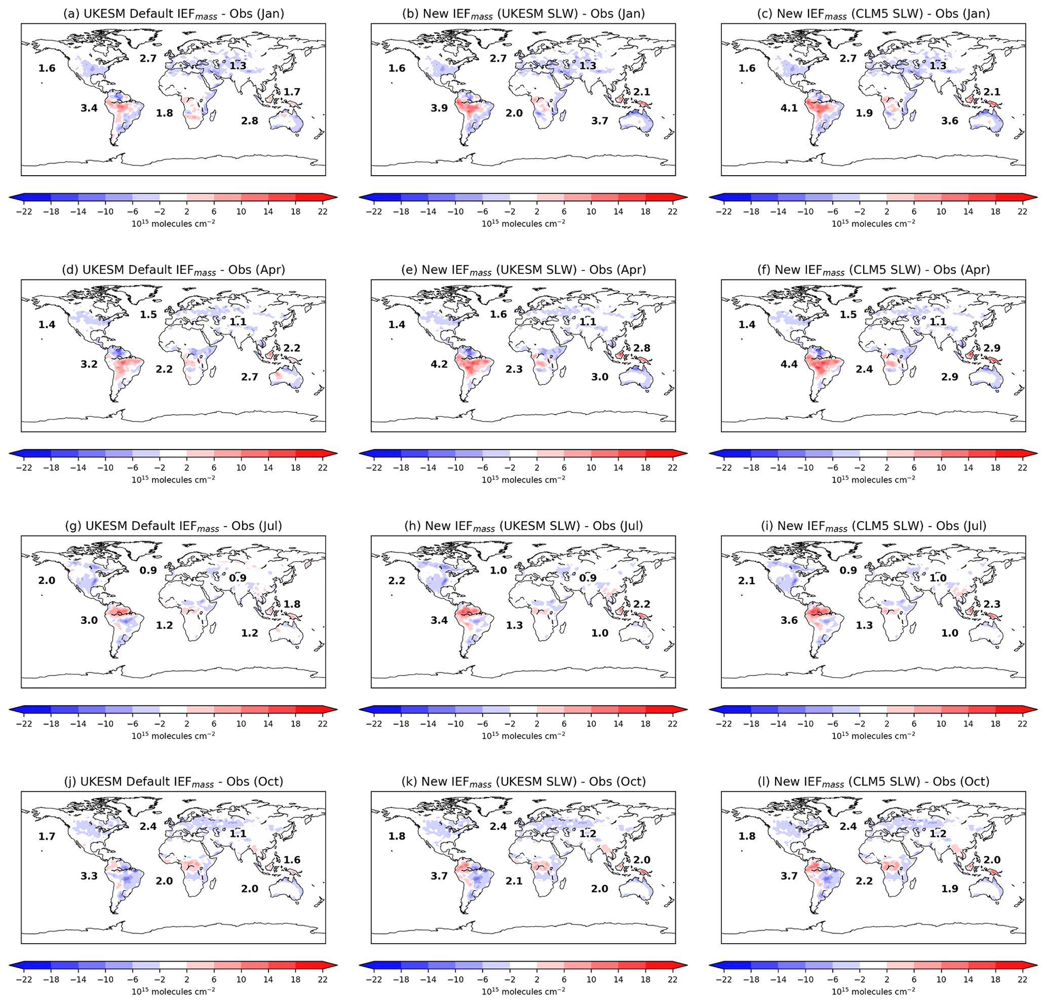
Figure 4 Modelled isoprene column compared to observational data (Wells et al., 2020) for (a–c) January 2013, (d–f) April 2013, (g–i) July 2013 and (j–l) October 2013. Model data from UKESM1 IEF_mass new IEF_mass (UKESM1 SLW) and new IEF_mass (CLM5 SLW) from Control_1yr_PD, IEF_SLW_UKESM_PD and IEF_SLW_CLM5_PD simulations respectively. Numbers show mean absolute bias (MAB = | model − obs |) weighted by area for each continent (the African value excludes the Sahara).

The increased biases with the new IEF_mass (e.g. the increase of 0.5–0.7 × 10¹⁵ molecules cm⁻² over South America in January 2013, Fig. 4a–c) is not necessarily indicative of these new IEF_mass values being less accurate than the original IEF_mass values which may be performing better due to offsetting issues. Biases in LULC, as highlighted by the comparison of UKESM1 and CLM5 in terms of broadleaf vs. deciduous tropical trees, simulated chemistry and emissions of other species (e.g. NO_x) which affect the atmospheric oxidising capacity and thus isoprene concentrations will also contribute to the enhanced model bias. The difference in model bias between simulations with the default and new IEF_mass values is noticeably smaller than the difference in the model bias when different chemical mechanisms are used. For example, in April 2013, the mean bias over South America in the Strat-Trop mechanism (Archibald et al., 2020) was 5.7 × 10¹⁵ molecules cm⁻², and this decreased substantially to 0.6 × 10¹⁵ molecules cm⁻² when CS2 was used (Fig. 2; Weber et al., 2021)

4.3 C₄ emission observation comparison

Given the major change to the IEF_mass values of C₄ grass, the isoprene emissions from C₄ grasses were compared to observations in southern Africa (Sect. 3.3, Fig. 5). The model resolution (∼ 100 × 100 km in the region of relevance) means the grid cells where observations were made contained high fractions of strong isoprene emitters, typically broadleaf evergreen tropical trees and C₄ grasses. To isolate the impact of C₄ grass emissions, we take the area-weighted mean of emissions from grid cells in the region where C₄ grasses comprise > 80 % of the total surface types (vegetation and non-vegetation). We use the 3-year monthly mean for the month when observations were recorded and apply a scaling factor of 2 to account for the fact that isoprene emissions are zero at night. (Emission measurements were only taken during the day, while the use of model monthly average values means that approximately half of the data points going into the model value will been zero, halving the model's average.)

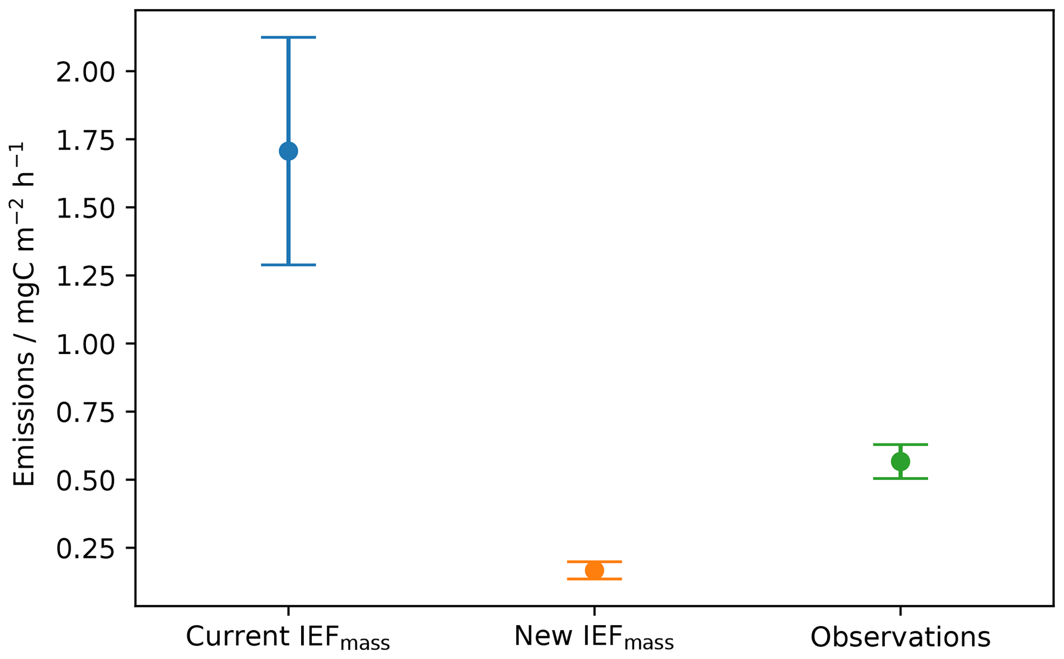
Figure 5 Simulated isoprene emissions from the IEF_mass currently used in UKESM1 and the new IEF_mass described in this study and observations. For the simulated emissions, we only consider grid cells with > 80 % C₄ grass located in the same regions as the observations.

While comparison of these model and observational data should be treated as illustrative rather than definitive for the reasons explained above, it suggests that the reduction in C₄ IEF_mass may help to reduce the model high bias in C₄-grass-dominant regions. We also note that the observed values represent an upper bound since the emissions in some regions will be below the limit of detection (e.g. Harley et al., 2003).

4.4 Terpene emission evaluation

While the primary focus of this paper is correcting the error with the emission factors for C₄ grasses, we also performed a comparison of monoterpene emissions measured by the SMEAR II station in Hyytiälä in the boreal forest, with emissions from simulations using the current TEF_mass (Control_1yr_PD) and updated TEF_mass (TEF_AP_BP_PD) values. We found that the new TEF_mass yielded emissions which compared well to observations (Fig. S2).

4.5 Impact on response to LULC changes

Tropical broadleaf evergreen trees and C₄ grass PFTs are some of the most widespread vegetation types in the tropics. The respective increase and decrease in EF_mass values for these PFTs means the response of BVOC emissions to a change in the relative fractions of these species is likely to be quite different when using default and new EF_mass values. We explored this further using UKESM1 and CESM and the MaxForest scenarios since this scenario involves, among other changes, increases to tropical broadleaf evergreen tree cover at the expense of C₄ grasses in Africa and eastern Brazil (Fig. S3 and Table 5).

When the UKESM1 default EF_mass values are used, the extensive reforestation/afforestation in the Maxforest scenario yields a reduction in isoprene emissions relative to 2010 (Fig. 6a). This is due to the decrease in C₄ grass coverage shown by emission reductions in regions where C₄ grasses are replaced by trees. By contrast, when the updated EF_mass values are used, the Maxforest scenario leads to an increase in isoprene emissions in UKESM1 (Fig. 6b) which resembles the response simulated in CESM (Fig. 6c). The similarity between the responses in UKESM1 to the new EF_mass and CESM is not surprising since CESM also uses the MEGAN v2.1 scheme for the emissions of isoprene.

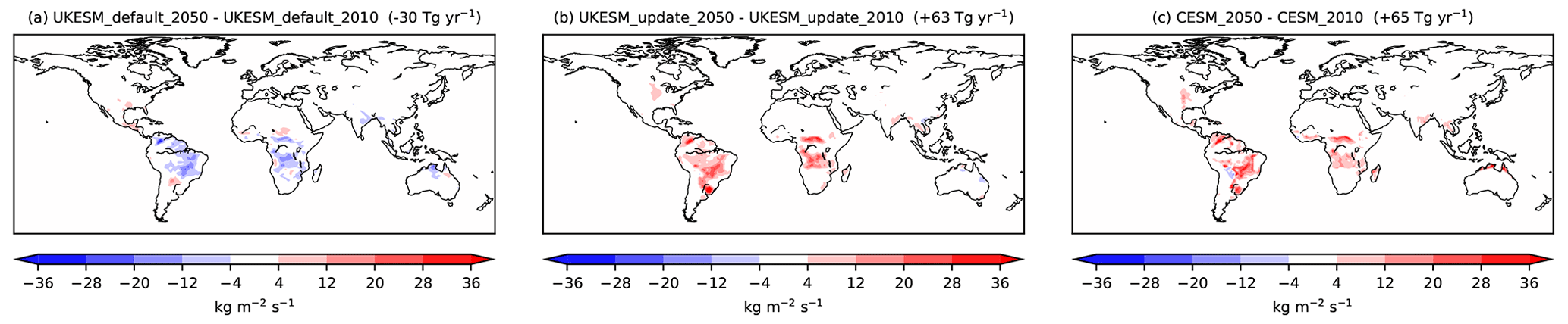
Figure 6 Annual mean change (2050 minus 2010) in isoprene emissions in the (a) original UKESM1, (b) UKESM1 with new IEF_mass and (c) CESM2 following widespread tree planting under the Maxforest scenario. Values in parentheses show the global mean difference in emissions.

4.6 Recommended EF_mass

For isoprene, there is little to differentiate the approaches using SLW from CLM5 or UKESM1. The CLM5 SLW approach yields slightly higher column biases but total PD emissions (491 vs. 457 Tg yr⁻¹; Table 4) which are closer to the median of other estimates (∼ 500 Tg yr⁻¹; Messina et al., 2016). The CLM5 SLW approach allows PFT-specific SLW values to be used to calculate the EF_mass of the MEGAN v2.1 PFTs before they are lumped into UKESM PFTs, while using the UKESM1 SLW values means lumping must occur before the EF_mass are calculated, potentially increasing uncertainty in the output. Overall, we tentatively recommend using the IEF_mass values calculated using the CLM5 values (i.e. IEF_SLW_CLM5_PD). For terpenes, based on total emissions we recommend the TEF_mass calculated from the TEF_area of α-pinene and β-pinene in a 2:1 ratio (Guenther et al., 2012), i.e. those used in TEF_all_PD. These EF_mass values are given in Table 6.

We do not claim that the new EF_mass values are the final word on the matter; rather, we believe that they represent an improvement over those currently used in UKESM1 and provide a clear method for recalculation in the future should revised EF_area values be developed and/or a wider range of PFTs considered.

Table 6 Recommended EF_mass (µgC g${}_{\mathrm{dw}}^{-\mathrm{1}}$ h⁻¹) for use in iBVOC.

4.7 Uncertainties and future work

Accurate modelling of BVOC emissions depends on the parameterisations within the emission module (in this case, iBVOC) and the simulations of external factors, which influence emissions. This study deals with just one part of this framework: biases in these external factors can limit the effectiveness of model–observation comparisons, such as the satellite-derived isoprene columns shown in Fig. 4, and offsetting errors can lead to reasonable results, at a given period in time, or improvements to certain components (e.g. emission factors) yielding reductions in model performance. Nevertheless, progress towards an approach that faithfully captures biosphere–atmosphere interactions requires incremental improvements to all contributing factors. Here we describe some other sources of uncertainty in the simulation of BVOCs and areas where future work would be useful.

iBVOC includes dependencies on CO₂, temperature, photosynthetic activity and plant functional type, with the latter the focus of this study. MEGANv2.1 considers the role of leaf age in emissions and leaf temperature over the past 24 and 240 h, while these factors are omitted in iBVOC: assessing the impact of these parameterisations in iBVOC would be worthwhile.

Within the parameterisation of PFT dependency updated in the study, several areas of uncertainty have been identified. The impact of SLW value variations and the multiple options regarding which TEF_area values to use have been quantified with the range of simulations performed in this work. Other areas of uncertainty have not been fully scrutinised due to a relative lack of observational data. Compared to the species which are strong isoprene emitters, observations of emissions from grasses are sparse, hindering further model validation. MEGAN v2.1 also prescribes a single, very small EF_area for all crops and pasture, resulting in negligible emissions from these PFTs. Emissions from longer-lived crops and pasture are likely to tend towards grasses and the projected expansion of these PFTs in some future scenarios, particularly those with increasing population, meaning that capturing emissions from these PFTs may become more important. Further observations would aid in this effort. We also note that the emission factors in MEGAN v2.1 are not perfect and will continue to be refined. For example, Sindelarova et al. (2022) updated emission factors for α-pinene for certain tree PFTs. For consistency, the MEGAN emission factors used in this study are all from MEGAN v2.1, but future development of iBVOC should take into account the latest understanding of emission factors.

Simulation of external factors including land cover (cf. the effect of swapping UKESM and CESM LULC on simulated emissions; Table 4), surface temperature and meteorological conditions (e.g. droughts and floods) also affect BVOC emissions (e.g. Sheil, 2018; Yáñez-Serrano et al., 2020).

The reduced nature of Earth system models requires the aggregation of a wide range of vegetation types, which in reality have varying emission factors, into a small number of PFTs. This oversimplification can lead to unrealistic emissions in certain locations (e.g. the inclusion of shrubs EF in grasses EF) and discrepancies between different modelling approaches (e.g. UKESM1 vs. CESM). Assessment of the impact of using a wider range of PFTs, based on more highly resolved emission factor datasets (e.g. Karl et al., 2009), would be informative.

The expansion of iBVOC to speciate terpenes into separate α-pinene and β-pinene tracers and the addition of new molecules, such as sesquiterpenes, would be beneficial for simulating atmospheric composition. α-pinene and β-pinene display different chemical reactivity, while sesquiterpenes can suppress local O₃ and affect SOA formation by producing highly involatile species which can nucleate new particles without sulfuric acid (e.g. Bianchi et al., 2019; Weber et al., 2020).

5 Conclusions

The influence of BVOC emissions on atmospheric composition and climate and the predicted changes in these emissions from climatic and land use drivers means accurate modelling is critical for understanding past, present and future climate.

In this study we have described the development and evaluation of alternative sets of emission factors (EF_mass) for isoprene and monoterpenes from the established MEGAN v2.1 scheme. This development rectifies the issue in the current UKESM1 set-up of the over-contribution to total isoprene emissions from C₄ PFTs, caused by the differences in the scope of vegetation types included in the C₃ and C₄ PFTs in UKESM1 and the previous source of emission factors, ORCHIDEE. The correction reduces the C₄ grass contribution to total isoprene emissions, bringing them into line with other literature. Meanwhile, EF_mass values for isoprene and terpene increase for the three broadleaf tree PFTs in UKESM1. This leads to the fraction of both isoprene and terpene produced by the tropical broadleaf evergreen tree increasing from ∼ 50 % to ∼ 80 %.

During the calculation, we identified variation in SLW datasets and the decision on which monoterpene emission factors to use as sources of uncertainty in the final EF_mass values. The high bias in simulated isoprene column values increases slightly with the updated IEF_mass values compared to the UKESM1 approach, although this change is much smaller than that caused by switching between chemical mechanisms.

When using the current UKESM1 EF_mass values, isoprene emissions decrease in future LULC scenarios featuring wide-scale tree planting relative to 2010 levels due to the erroneously high IEF_mass of C₄ grass. When the new EF_mass values are used, isoprene emission increases and UKESM's response agrees closely with the response simulated by CESM. Thus, the increase in EF_mass for tropical trees and the reduction for C₄ grass PFTs are likely to have consequences for the evolution of isoprene emissions under different future scenarios given the competition between C₄ grass PFTs and tropical broadleaf evergreen trees (e.g. cropland expansion vs. reforestation/afforestation efforts).