iHydroSlide3D v1.0: an advanced hydrological–geotechnical model for hydrological simulation and three-dimensional landslide prediction

Forecasting flood–landslide cascading disasters in flood- and landslide-prone regions is an important topic within the scientific community. Existing hydrological–geotechnical models mainly employ infinite or static 3D stability models, and very few models have incorporated the 3D landslide model into a distributed hydrological model. In this work, we modified a 3D landslide model to account for slope stability under various soil wetness states and then coupled it with the Coupled Routing and Excess STorage (CREST) distributed hydrology model, forming a new modeling system called iHydroSlide3D v1.0. Through embedding a soil moisture downscaling method, this model is able to model hydrological and slope-stability submodules even at different resolutions. For a large-scale application, we paralleled the code and elaborated several computational strategies. The model produces a relatively comprehensive and reliable diagnosis for flood–landslide events, including (i) complete hydrological components (e.g., soil moisture and streamflow), (ii) a landslide susceptibility assessment (factor of safety and probability of occurrence), and (iii) a landslide hazard analysis (geometric properties of potential failures). We evaluated the plausibility of the model by testing it in a large and complex geographical area, the Yuehe River basin, China, where we attempted to reproduce cascading flood–landslide events. The results are well verified at both hydrological and geotechnical levels. iHydroSlide3D v1.0 is therefore appropriately used as an innovative tool for assessing and predicting cascading flood–landslide events once the model is well calibrated.

1 Introduction

Landslides represent mass-movement processes in hilly and mountainous environments and pose significant threats to human lives and properties (Hong et al., 2006; He et al., 2016). Rainfall events characterized by short-duration but high-intensity precipitation can substantially change the soil state of unlithified soil mantle or regolith (Srivastava and Yeh, 1991; Iverson, 2000; Baum et al., 2010) and thus affect hillslope stability and cause flash floods in channels. Forecasting flood–landslide hazards and correspondingly evacuating people from hazardous zones in advance are widely regarded as a critical risk reduction strategy (Abraham et al., 2021). However, to date, it is still challenging to accurately and reasonably forecast the landslides due to the complex natural processes and the interweaving hydrological, geomorphic, and geotechnical mechanisms (Sidle and Bogaard, 2016; Guzzetti, 2021).

Modeling landslide susceptibility can be appropriately accomplished by adopting a variety of approaches, including statistical methods (Guzzetti et al., 2007; Segoni et al., 2018), physically based models (Baum et al., 2010; He et al., 2016; Zhang et al., 2016), and geotechnical approaches (van Westen et al., 2006), among others. Among them, the deterministic and physically based models (PBMs) are popularly used for modeling the spatiotemporal susceptibility of landslides. Some of these approaches attempt to define a direct correlation between rainfall depth and slope stability under some simplified hypotheses (Montrasio and Valentino, 2008; Liao et al., 2010). These models are useful for regional landslide stability assessment but fail to reproduce cascading flood–landslide disasters in catchments. More recently, efforts have been devoted to coupling the sound hydrological models with more or less complex landslide models (Baum and Godt, 2010; Lepore et al., 2013; He et al., 2016; Zhang et al., 2016; Aristizábal et al., 2016; Wang et al., 2020). Literature has shown the contributions of hydrological–geotechnical models to real-world applications, such as improvements of disaster preparedness and hazard management in North Carolina, US (Zhang et al., 2016), and long-term vulnerability estimates in Shaanxi Province, China (Wang et al., 2020), to name a few. These models include physical representations of precipitation, evapotranspiration, infiltration with continuous soil moisture accounting, runoff routing, and the slope-stability module. However, most of them rely on infinite slope-stability models (i.e., one-dimensional models), which are based on the assumption of planar shallow failures and fail to capture the complexity of landslide geometry in many landscapes where shallow- and deep-seated landslides inherently coexist (Zêzere et al., 2005; Mergili et al., 2014b; Tran et al., 2018). To this end, three-dimensional slope-stability models (3D models) are proposed to cope with more complex scenarios (Mergili et al., 2014a; Reid et al., 2015).

Until now, as reviewed by Vandromme et al. (2020), the existing hazard software for the implementation of spatial PBMs mainly employs the one-dimensional (1D) or two-dimensional (2D) methods for slope-stability calculation. The 3D approaches like Scoops3D (Reid et al., 2015) and r.slope.stability (Mergili et al., 2014a) are only practical for static conditions such as imposed water level and fully saturated soil state. Researchers have attempted to combine the hydrological part of the Transient Rainfall Infiltration and Grid-Based Regional Slope-Stability (TRIGRS, a well-known, publicly available software) model (Baum et al., 2010) with a 3D model and analyzed the hillslope stability on a regional scale (Tran et al., 2018; He et al., 2021). To date, there are still very few fully coupled hydrological–geotechnical models capable of performing at large scales and producing 3D information of landslide disasters. The progress is hindered by complicated model structures and considerable computational loads. The latter is inevitable and is an inherent feature for PBMs when the applications are conducted at a large scale using the 3D models (Zieher et al., 2017). Another problem is the selection of computational spatial resolutions. Hydrological modeling with a coarse spatial resolution (e.g., 1 km resolution or coarser) but a large-scale coverage has been widely available with the increasing availability of meteorological and land surface data (X. Xue et al., 2013; Chao et al., 2019, 2021). However, such a resolution is insufficient to capture the slope failures on hillslope scales, particularly for the landslide events that usually occur within an area of only tens or hundreds of square meters (Chen et al., 2017). Moreover, it is not wise to unlimitedly refine the mesh resolution of the hydrological model over a relatively large region. A strategy to tackle the differential needs for computational resolutions among the submodules is essential (Wang et al., 2020).

A comprehensive assessment for landslide disasters is generally composed of three parts (Vandromme et al., 2020): a landslide inventory, a landslide susceptibility analysis (usually denotes factor of safety (FS) and probability of occurrence), and a landslide hazard analysis (i.e., magnitude that takes into account the area and volume of failure). Among them, the landslide hazard analysis is not very common as the ordinary 1D models cannot represent the geometric properties of landslides. Previous studies for this purpose are more inclined to use available landslide datasets (Guzzetti et al., 2009; Brunetti et al., 2009; Klar et al., 2011) and advanced sensing and photogrammetric methods and techniques (e.g., aerial photograph interpretation, high-resolution imagery, and lidar interpretation) (Lacroix, 2016). However, in many cases, the landslide data are not well documented or insufficient data are unfavorable to support such analysis (e.g., only failure locations are recorded). Performing the landslide hazard analysis in such cases is necessary but difficult to implement.

In this work, we developed an innovative physically based integrated hydrological processes and 3D slope-stability modeling framework, which is called the integrated Hydrological processes and 3-Dimensional landSlide prediction model (iHydroSlide3D v1.0), by coupling a distributed hydrological model with a newly developed 3D geotechnical model. To alleviate the chronic contradiction of mesh resolutions required for hydrological and landslide simulations, we adopted the soil downscaling method to handle the soil moisture. iHydroSlide3D v1.0 is built on a parallel computational design, allowing the code to run efficiently on a multi-core machine. The code was tested in a large and complex geographical area, the Yuehe River basin of western China, where we attempted to reproduce cascading flood–landslide events.

The paper is organized as follows. We first describe the basic theories of submodules and main features of the framework in Sect. 2. In addition, we also elaborate the strategies for model implementation in Sect. 2. In Sect. 3, we introduce a case study and associated materials required for model simulation and evaluation. The results, primarily focused on the evolution processes of cascading flood–landslide events triggered by a rainstorm, are presented in Sect. 4. Finally, we discuss the results and summarize the conclusions in Sect. 5.

2 The integrated hydrological–geotechnical model framework: iHydroSlide3D v1.0

2.1 Overall structure

iHydroSlide3D v1.0 is a physically based modeling framework that accounts for both hydrological and geotechnical processes. The model mainly includes the following modules: (i) a distributed hydrological model based on the Coupled Routing and Excess STorage (CREST) model, (ii) a newly developed 3D landslide model, and (iii) a soil moisture downscaling method. The model can currently process two sets of data with different resolutions, allowing us to simultaneously model hydrological and geotechnical processes with different spatial resolutions. iHydroSlide3D v1.0 is coded in MATLAB and is capable of running in a parallel manner, currently supported by the Linux and Windows operating systems. Detailed descriptions of the model are presented as follows.

2.2 Hydrological model: the Coupled Routing and Excess STorage model

A physically based hydrological model, i.e., the Coupled Routing and Excess STorage (CREST) (Wang et al., 2011; Khan et al., 2011; Shen et al., 2016; X. W. Xue et al., 2013), is adopted to simulate hydrological processes that trigger the rainstorm-induced landslide events. The CREST model was first developed by the University of Oklahoma (http://hydro.ou.edu, last access: 23 December 2014) and NASA SERVIR project team (http://www.servir.net, last access: 15 September 2016) and served for predictions of flash floods caused by rainfalls on its early-version stage (Wang et al., 2011). The model is further enhanced by considering the Multi-Radar Multi-Sensor (MRMS) forcing data and has been used for hydroclimatology studies such as extreme hydrological events (e.g., floods and droughts) (Zhang et al., 2015; Khan et al., 2011) and statistical and hydrological evaluation in ungauged basins (X. Xue et al., 2013). The CREST model is run in a distributed fashion via a cell-to-cell design concept, while the coupling between overland flow generation and routing scheme allows a realistic and detailed simulation of hydrological variables such as soil moisture, which plays a major role in determining the stability of a slope. More recently, several coupled hydrological–geotechnical models based on the CREST model such as CRESLIDE (He et al., 2016) and iCRESTRIGRS (Zhang et al., 2016) have emerged as the application evolves. These models, counting on the hydrological simulation of the CREST model, have achieved their capability of back calculation and/or prediction for rainfall-triggered landslides. As a consequence, CREST has been comprehensively and extensively evaluated regarding its hydrological simulation skill and its flexibility for coupling. A detailed description of the CREST model can be found in Wang et al. (2011). For better understanding the work of this study, it is still important to briefly review the principal theories of the CREST model here.

The CREST model is driven by precipitation and potential or actual evapotranspiration. The rainfall–runoff-generation processes are computed at each cell, starting with accounting for its received precipitation at each time step (P). After P passes the canopy layer and deducts canopy interception, the excess precipitation (P_soil) then reaches the soil surface. A conceptual variable infiltration curve (VIC), originated from the Xinanjiang model (Zhao, 1992) and later adopted by the VIC model (Liang et al., 1994), is used to further divide the P_soil into excess rain (R) and infiltration water (I). The CREST model assumes that each soil column is capable of storing a maximum water depth, which is regarded as the infiltration capacity (i) and varies over an area in the following relationship:

$$\begin{array}{}\text{(1)}& i=i_{\mathrm{m}}\left[\mathrm{1}-(\mathrm{1}-a{)}^{\frac{\mathrm{1}}{b}}\right],\end{array}$$

where the i_m is the maximum infiltration capacity of a cell and strongly depends on the soil properties, a is a fraction number of a grid cell, and b is an empirical shape parameter. Under this assumption, the amount of water available for excess rain (R) and infiltration (I) can be further expressed as

$$\begin{array}{}\text{(2)}& {\displaystyle }I=\left\{\begin{array}{l}{W}_{\mathrm{m}}-W,i+P_{\text{soil}}\ge i_{\mathrm{m}}\\ (W_{\mathrm{m}}-W)+W_{\mathrm{m}}\cdot {\left[\mathrm{1}-\frac{i+P_{\text{soil}}}{i_{\mathrm{m}}}\right]}^{\mathrm{1}+b},i+P_{\text{soil}}<i_{\mathrm{m}},\end{array}\right.\text{(3)}& {\displaystyle }R=P_{\text{soil}}-I,\end{array}$$

where W_m denotes the maximum water capacity of a cell and W represents the total mean water of the three soil layers. R can be further partitioned into overland and subsurface flows by comparing P_soil to the infiltration rate of the first layer (K), which is closely related to the soil saturated hydraulic conductivity (K_sat). Then CREST adopts the multi-linear reservoir method to simulate the cell-to-cell routing of overland and subsurface runoff at each time step. The model can better take into account the interaction between the surface and subsurface flows by coupling the runoff-generation process and the routing scheme (Wang et al., 2011).

2.3 Three-dimensional stability model based on sliding surface

The 3D slope-stability analysis model was originally derived to describe the characteristics of a potential failure (Hovland, 1979). This model has no iteration procedure but computes the FS directly compared to the slope-stability models established based on Bishop (1955) and Janbu et al. (1956). Embedded in the geographic information system (GIS), the model composes a slope failure with column units, expressed as grid cells in GIS (software like 3DSlopeGIS) (Xie et al., 2003, 2004, 2006). More recently, progress has been made in a more sophisticated software r.slope.stability (Mergili et al., 2014a, b) that has the capacity to perform on a regional scale via a parallel computational technique. More importantly, the 3D slope-stability model has proven to be effective on both shallow and deep landslides and thus behaves better as a robust geotechnical tool and has potential for wide applications (Zieher et al., 2017; Palacio Cordoba et al., 2020).

However, to implement on a large scale, the previous versions of the 3D stability model treat the hydrological component (e.g., transient soil moisture and water level) as static or imposed inputs, failing to consider the time-dependent hydrological processes (Mergili et al., 2014b, a). In this work, the model is extended to take into account spatiotemporal variations of water fluxes and storages on regular grids by introducing the hydrological module. Following an assumption of being ellipsoidal or truncated in shape, the potential slope failures are randomly generated over a whole study region. When applied in a regional assessment, the theory of the model can be mainly divided into the following two parts.

2.3.1 Coordinate transformation and geometric derivation

Three levels of the coordinate system involved in this model are the (i) GIS coordinate system ($x,y,z$) over the whole study area (Fig. 1), (ii) Cartesian coordinate ($x^{\prime },y^{\prime },z^{\prime }$) of each potential failure, and (iii) ellipsoid coordinate system ($x^{\prime \prime },y^{\prime \prime },z^{\prime \prime }$) along the direction of the steepest slope in a single ellipsoid. The center of each ellipsoid ($x_{\mathrm{c}},y_{\mathrm{c}},z_{\mathrm{c}}$) is randomly generated within the study area, while the GIS coordinate system is simultaneously transformed to the Cartesian coordinate from a ground perspective (Mergili et al., 2014b):

$$\begin{array}{}\text{(4)}& {\displaystyle }{x}^{\prime }=(x-x_{\mathrm{c}})\cos \mathit{\alpha }+(y-y_{\mathrm{c}})\sin \mathit{\alpha },\text{(5)}& {\displaystyle }{y}^{\prime }=(y-y_{\mathrm{c}})\cos \mathit{\alpha }-(x-x_{\mathrm{c}})\sin \mathit{\alpha },\end{array}$$

where α is the main dip direction of the ellipsoid, x^′′ is easily derived as $x^{\prime \prime }=\frac{x^{\prime }}{\text{cos}\mathit{\beta }}$ (β is the main inclination of the ellipsoid; see Fig. 2), y^′′ is identical to the y^′ axis, and z^′ is identical to the z axis (Fig. 1). Then we need to filter the grid cells encompassed by this random ellipsoid, meeting the following condition:

$$\begin{array}{}\text{(6)}& {\displaystyle \frac{x^{\prime }}{a_{\mathrm{e}}^{\mathrm{2}}}}+{\displaystyle \frac{y^{\prime }}{b_{\mathrm{e}}^{\mathrm{2}}}}\le \mathrm{1},\end{array}$$

where a_e and b_e are half axes of the ellipsoid, following the x^′′ and y^′′ axes, respectively. These geometric lengths are randomly generated within user-defined ranges. To facilitate the derivation, we give a value of another half axis of the ellipsoid (c_e) beforehand, which is highly dependent on failure depth and should be reconsidered in following sections. Hence, with regard to an ideal ellipsoid, the above variables need to satisfy the basic equation of the ellipsoid:

$$\begin{array}{}\text{(7)}& {\displaystyle \frac{(x^{\prime \prime }+\mathrm{\Delta }{x}^{\prime \prime }{)}^{\mathrm{2}}}{a_{\mathrm{e}}^{\mathrm{2}}}}+{\displaystyle \frac{y^{\prime \prime \mathrm{2}}}{b_{\mathrm{e}}^{\mathrm{2}}}}+{\displaystyle \frac{\mathrm{\Delta }{x}^{\prime \mathrm{2}}}{c_{\mathrm{e}}^{\mathrm{2}}(\text{tan}\mathit{\beta }{)}^{\mathrm{2}}}}=\mathrm{1}.\end{array}$$

Figure 1 Coordinate systems involved in an arbitrary ellipsoid.

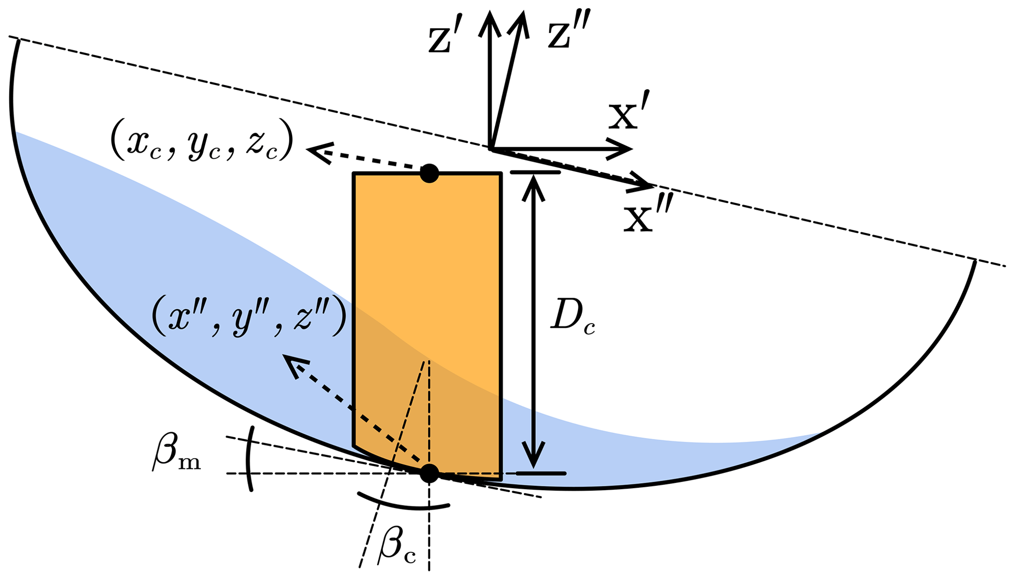
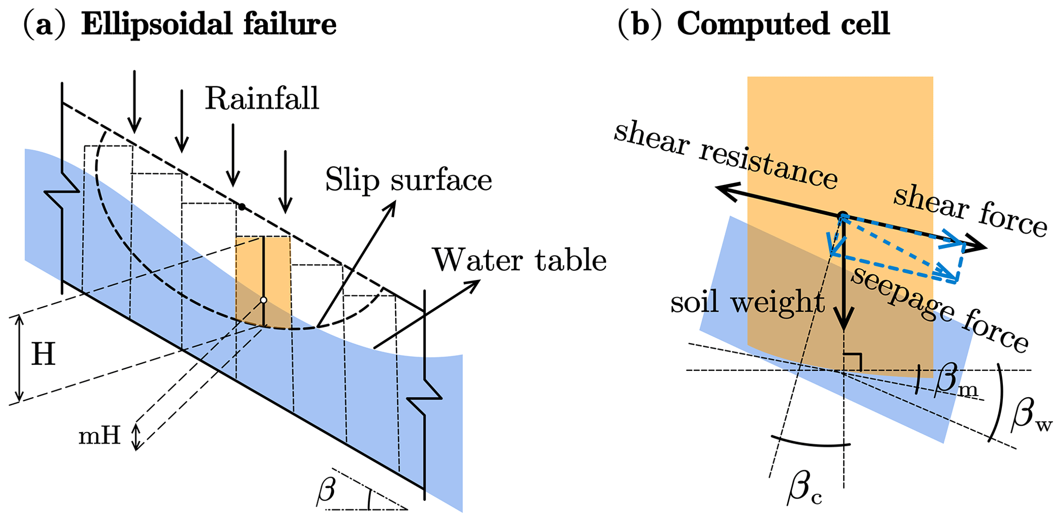
Figure 2 Typical longitudinal section of an ellipsoid used as slip surface in iHydroSlide3D v1.0: (a) overall features involved in a potential failure and (b) forces acting at each column considering the groundwater effect.

By solving the intermediate variable Δx^′′, the z^′′ can be computed as

$$\begin{array}{}\text{(8)}& z^{\prime \prime }={\displaystyle \frac{\mathrm{\Delta }{x}^{\prime \prime }}{\tan \mathit{\beta }}}.\end{array}$$

Finally, we transformed it back into the GIS coordinate system:

$$\begin{array}{}\text{(9)}& z_{\text{slip}}=z_{\mathrm{c}}+{\displaystyle \frac{(z^{\prime \prime }-x^{\prime }\sin \mathit{\beta })}{\cos \mathit{\beta }}},\end{array}$$

where z_slip is the elevation of the considered cell in the ellipsoid. We get all coordinates once a random ellipsoid is generated. We further note that such a procedure is required for each random ellipsoid (i.e., each random loop) and thus is time-consuming particularly in a regional map system. The countermeasures will be introduced in the following sections.

2.3.2 Basic hydrogeological mechanics

This study adopted a conceptual parameter m to better simulate the soil moisture of each considered column in a random ellipsoid (see Fig. 2). The parameters originated from Montrasio and Valentino (2008) and were later represented in further applications (Liao et al., 2010; He et al., 2016). The parameter m is a distributed value ranging from 0 to 1 and is controlled by hydrologic mechanisms (Fig. 2), which further impacts the matric suction and results in occurrences of landslides (Baum et al., 2010). More specifically, the apparent cohesion is strongly dependent on matric suction, which in turn is related to the degree of saturation of the soil column (S_r) (Montrasio and Valentino, 2008):

$$\begin{array}{}\text{(10)}& c_{\mathit{\psi }}\left(t\right)=\mathit{\delta }\cdot S_{\mathrm{r}}\cdot (\mathrm{1}-S_{\mathrm{r}}{)}^{\mathit{\lambda }}\cdot (\mathrm{1}-m{)}^{\mathit{\alpha }},\end{array}$$

where δ is a soil-type parameter and mainly refers to the peak shear stress at a failure layer; α and λ are numerical parameters to estimate the extreme points of the shear strength curve versus S_r and versus the degree of saturation of the soil, respectively. Then the total cohesion (C^′) is computed as follows:

$$\begin{array}{}\text{(11)}& C^{\prime }=c^{\prime }+c_{\mathit{\psi }}\left(t\right),\end{array}$$

where c^′ is effective cohesion depending on soil type and is treated as a constant value associated with each grid cell. The failures may take place in both partially and fully saturated scenarios (Lu and Likos, 2006; Lu and Godt, 2013); the latter should take the seepage force (S) into account (Collins and Znidarcic, 2004). Considering the inter-slice forces in this model, the seepage force is computed according to the hydraulic gradient, reflecting a more general situation in the hillslope (King, 1989; Mergili et al., 2014b). Note that the seepage force is only considered in soil columns satisfying m>0. Besides, the grid cell that has a low elevation is excluded from the considered ellipsoid by comparing z_slip and z_c:

$$\begin{array}{}\text{(12)}& D_{\mathrm{c}}=z_{\mathrm{c}}-z_{\text{slip}}.\end{array}$$

For the soil column satisfying both of the conditions, m>0 and D_c>0, the seepage force can be approximated by the slope (β_w) and aspect (α_w) of the groundwater table (Fig. 2), acting in the direction of the hydraulic gradient (Mergili et al., 2014b, a):

$$\begin{array}{}\text{(13)}& S={\mathit{\gamma }}_{\mathrm{w}}\cdot \mathrm{d}x\cdot \mathrm{d}y\cdot mH\cdot \text{sin}{\mathit{\beta }}_{\mathrm{w}},\end{array}$$

where γ_w is the specific weight of water and dx and dy are the cell size, depending on the resolution of input data. To further transfer the seepage force from hydraulic gradient to sliding direction, S is first divided into horizontal (S_h) and vertical (S_v) components (Fig. 2):

$$\begin{array}{}\text{(14)}& S_{\mathrm{h}}=S\text{cos}{\mathit{\beta }}_{\mathrm{w}}\text{ and }{S}_{\mathrm{v}}=S\text{sin}{\mathit{\beta }}_{\mathrm{w}}.\end{array}$$

S_v is irrelevant to the direction, while S_h needs to be further projected according to the dip direction of grid column (α_c) and the main inclination direction of the slip surface given by

$$\begin{array}{}\text{(15)}& S_{\text{ch}}=S_{\mathrm{h}}\text{cos}({\mathit{\alpha }}_{\mathrm{w}}-{\mathit{\alpha }}_{\mathrm{c}})\text{ and }{S}_{\text{mh}}=S_{\mathrm{h}}\text{cos}({\mathit{\alpha }}_{\mathrm{w}}-\mathit{\alpha }).\end{array}$$

Conforming to the orthogonality rule, the projected seepage force (S_c,S_m) and its vertical angle (${\mathit{\beta }}_{S_{\mathrm{c}}},{\mathit{\beta }}_{S_{\mathrm{m}}}$) can be expressed as

$$\begin{array}{}\text{(16)}& \begin{array}{r}{S}_{\mathrm{c}}=\sqrt{S_{\mathrm{v}}^{\mathrm{2}}+S_{\text{ch}}^{\mathrm{2}}};S_{\mathrm{m}}=\sqrt{S_{\mathrm{v}}^{\mathrm{2}}+S_{\text{mh}}^{\mathrm{2}}}\\ \cos {\mathit{\beta }}_{S_{\mathrm{c}}}={\displaystyle \frac{S_{\text{ch}}}{S_{\mathrm{c}}}};{\mathit{\beta }}_{S_{\mathrm{m}}}={\displaystyle \frac{S_{\text{mh}}}{S_{\mathrm{m}}}}.\end{array}\end{array}$$

The final expression of the seepage force acting on each grid column can be written as normal and slope-parallel components:

$$\begin{array}{}\text{(17)}& N_{\mathrm{s}}=S_{\mathrm{c}}\sin ({\mathit{\beta }}_{S_{\mathrm{c}}}-{\mathit{\beta }}_{\mathrm{c}});T_{\mathrm{s}}=S_{\mathrm{m}}\cos ({\mathit{\beta }}_{S_{\mathrm{m}}}-{\mathit{\beta }}_{\mathrm{m}}).\end{array}$$

The soil weight (G^′), considering the variant degree of saturation and under the condition of D_c>0, is derived as

$$\begin{array}{}\text{(18)}& G^{\prime }=\mathrm{d}x\cdot \mathrm{d}y\cdot [y_{\mathrm{d}}{D}_{\mathrm{c}}+y_{\mathrm{w}}\cdot mH\cdot (n-\mathrm{1})+y_{\mathrm{w}}(D_{\mathrm{c}}-mH\left)n{S}_{\mathrm{r}}\right],\end{array}$$

where γ_d is the unit weight of the dry soil; n and S_r represent the porosity and soil saturation degree, respectively. Based on the limited equilibrium condition, the model assesses the critical scenarios by calculating the FS, which can be mechanically subject to the stabilizing and destabilizing actions. Summarizing the derivations above, the extended version of the 3D slope-stability equation can be written as follows:

$$\begin{array}{}\text{(19)}& \mathrm{FS}={\displaystyle \frac{\begin{array}{c}\sum _c[\left(C^{\prime }+\mathit{\delta }\cdot S_{\mathrm{r}}\cdot (\mathrm{1}-S_{\mathrm{r}}{)}^{\mathit{\lambda }}\cdot (\mathrm{1}-m{)}^{\mathit{\alpha }}\right)\cdot A\\ +\left(G^{\prime }\text{cos}{\mathit{\beta }}_{\mathrm{c}}+N_{\mathrm{s}}\right)\text{tan}\mathit{\phi }]\cos {\mathit{\beta }}_{\mathrm{m}}\end{array}}{\sum _c\left(G^{\prime }\sin {\mathit{\beta }}_{\mathrm{m}}+T_{\mathrm{s}}\right)\cos {\mathit{\beta }}_{\mathrm{m}}}},\end{array}$$

where φ is the friction angle; β_c and β_m denote the dip and apparent dip of the slip surface at a considered soil column, respectively; and A is the slip surface area of each column and can be computed as

$$\begin{array}{}\text{(20)}& A=\mathrm{d}x\cdot \mathrm{d}y{\displaystyle \frac{\sqrt{\mathrm{1}-\left(\sin {\mathit{\beta }}_{xz}{)}^{\mathrm{2}}\right(\sin {\mathit{\beta }}_{yz}{)}^{\mathrm{2}}}}{\cos {\mathit{\beta }}_{xz}\cos {\mathit{\beta }}_{yz}}},\end{array}$$

where β_xz and β_yz are apparent dips of the x and y axis, respectively. The relationships between the apparent dips and main sliding direction assigned to each soil column can be expressed as (Xie et al., 2003)

$$\begin{array}{}\text{(21)}& \begin{array}{rl}& \tan {\mathit{\beta }}_{\mathrm{m}}=\tan {\mathit{\beta }}_{\mathrm{c}}\mathrm{|}\cos ({\mathit{\alpha }}_{\mathrm{c}}-\mathit{\alpha })\mathrm{|},\\ & \tan {\mathit{\beta }}_{xz}=\tan {\mathit{\beta }}_{\mathrm{c}}\sin {\mathit{\alpha }}_{\mathrm{c}},\\ & \tan {\mathit{\beta }}_{yz}=\tan {\mathit{\beta }}_{\mathrm{c}}\cos {\mathit{\alpha }}_{\mathrm{c}}.\end{array}\end{array}$$

The model diagnoses whether the landslide is stable or not by comparing the value of FS with a critical value that usually set to 1. At the same time, for each random ellipsoid, the volume and area of a failure can be approximated by

$$\begin{array}{}\text{(22)}& {\displaystyle }{V}_{\mathrm{L}}=\sum D_{\mathrm{c}}\cdot \mathrm{d}x\cdot \mathrm{d}y,\text{(23)}& {\displaystyle }{A}_{\mathrm{L}}=\sum \mathrm{d}x\cdot \mathrm{d}y.\end{array}$$

It is noteworthy that the 3D stability model can function independently by directly incorporating soil moisture and groundwater table information. However, in a more practical sense, the landslide model is coupled with the hydrological model.

2.4 Soil moisture downscaling method

A near-conservative downscaling method of soil moisture (Droesen, 2016; Wang et al., 2020) is adopted here to link different-resolution-based submodules in iHydroSlide3D v1.0, i.e., the relatively coarse-resolution hydrological model and the fine-resolution 3D slope-stability model. The method relates the soil moisture with the topographic wetness index (TWI) by proposing a conversion parameter, the wetness coefficient (K_w). The relationship between K_w and TWI at the coarse resolution (K_w,coarse and TWI_coarse) is first detected, and the concave and convex areas are also distinguished. Then this relation is used to calculate K_w and TWI at the fine resolution (K_w,fine and TWI_fine), which is further used to fix the soil moisture at fine resolution. Readers may refer to Wang et al. (2020) for more detailed descriptions. This method helps the hydrological module produce soil moisture with a higher resolution that can be seamlessly utilized by the landslide module. The method has demonstrated its effectiveness (Wang et al., 2020) and is necessary for a hydrogeological-type model to balance the tedious computational tasks and accuracy.

Figure 3 Flowchart illustrating the work process of iHydroSlide3D v1.0.

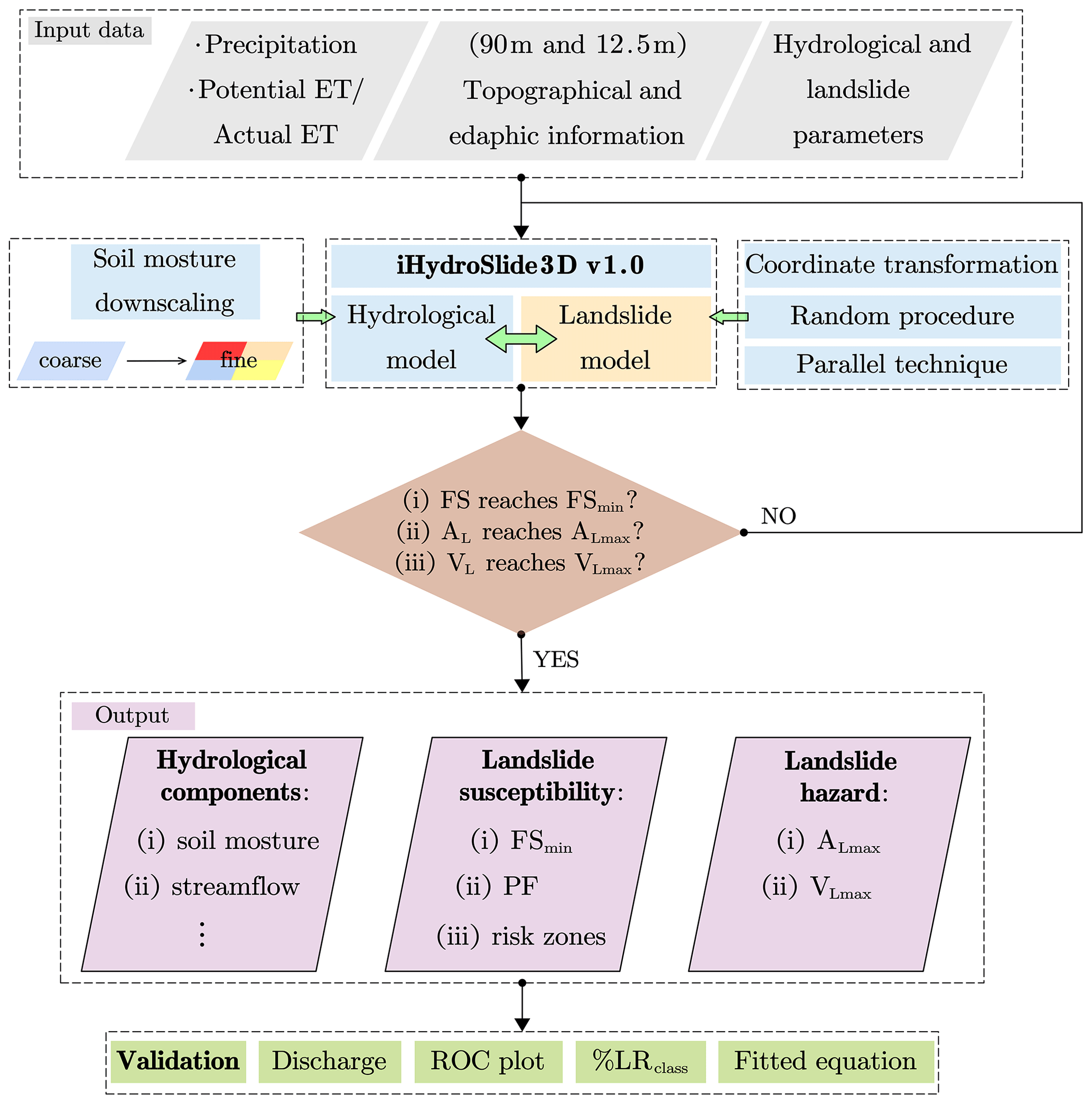
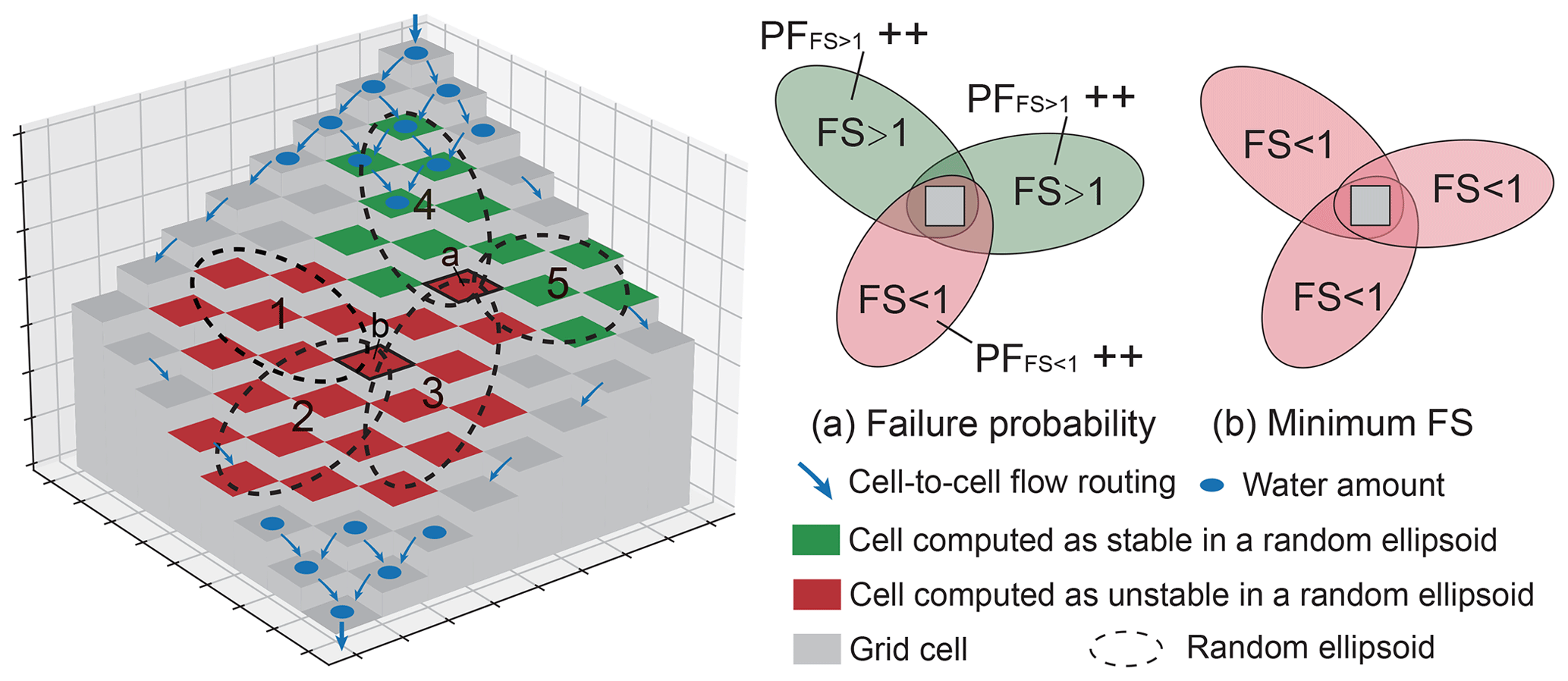
Figure 4 Cell-to-cell routing scheme and potential landslides generated across the grid in iHydroSlide3D v1.0: panels (a) and (b) illustrate the definitions of PF and FS within the framework, respectively.

2.5 Coupling strategy and model implementation

iHydroSlide3D v1.0 mainly consists of three sub-modules: (i) the hydrological model CREST, (ii) the soil moisture downscaling method, and (iii) the 3D landslide-stability model (Fig. 3). The CREST model undertakes the complete computational tasks of hydrologic processes, including interception by vegetation, water infiltration, runoff generation, cell-to-cell routing, and re-infiltration on each grid cell in the course of excess surface runoff moving from upstream to downstream, of which the infiltration and re-infiltration play the most important role on the coupled hydrology–slope-stability processes. The landslide model inherits the hydrological variables from the hydrological model and acts as a slope-stability monitor. The complete simulation cycle is seamlessly facilitated by the downscaling module. To elucidate the implementation of iHydroSlide3D v1.0, we present the logical framework in Fig. 3 and summarize the detailed coupling strategy in the following.

1. Instead of directly linking the soil moisture with rainfall intensity, the model takes the water loss into account due to the interception and evapotranspiration. The hydrological module helps to better simulate antecedent conditions such as soil moisture and cumulative infiltration. As a consequence, the parameter m is updated as a spatiotemporal variable (m_t) (He et al., 2016):

   $$\begin{array}{}\text{(24)}& m_{\mathrm{t}}={\displaystyle \frac{W_{\mathrm{t}}}{n{D}_t(\mathrm{1}-S_{\mathrm{r}})}},\end{array}$$

   where W_t is the mean water amount of the three soil layers on a given grid cell. S_r can be computed as

   $$\begin{array}{}\text{(25)}& S_{\mathrm{r}}={\displaystyle \frac{W_{\mathrm{t}}}{W_{\mathrm{m}}}}.\end{array}$$

   D_t is the landslide's initiation depth for various soil states and is largely impacted by soil heterogeneity and hydraulic properties (Lu and Godt, 2008). Therefore, D_t is determined by infiltration processes at time t (He et al., 2016):

   $$\begin{array}{}\text{(26)}& D_t=\sqrt{{\displaystyle \frac{\mathrm{2}{K}_{\mathrm{s}}{H}_{\mathrm{c}}t}{{\mathit{\theta }}_{\mathrm{n}}-{\mathit{\theta }}_{\mathrm{0}}}}},\end{array}$$

   where K_s is saturated hydraulic conductivity, H_c is capillary pressure, θ_n is volumetric water content of the saturated soil, and θ₀ is initial water content of the soil. Note that m_t, S_r, and D_t are gridded values.

2. We prepare two sets of data with different resolutions: a relatively coarser hydrological resolution and a finer landslide resolution. Once the soil moisture is calculated for all coarser grid cells, the soil moisture downscaling module is activated to calculate a new soil moisture map in a finer resolution to fit the spatial resolution of the landslide model (SM_Hydro→SM_Land).

3. In each simulation time step, the model generates a large number of ellipsoidal tested landslides with a random geometric center and ellipsoid length and width. The latter is constrained by the range of maximum and minimum values, which are determined from field investigation and regarded as the input parameters. Each random ellipsoid adopts maximum soil depth as another geometric length (c_e) among the encompassed cells ($D_t=max\mathit{\{}{D}_{\text{cell1}},D_{\text{cell2}},D_{\text{cell3}},\mathrm{\dots }\mathit{\}}$). The coordinate transformation and related geometric derivation are then tackled according to Sect. 2.3.1. Next, each tested landslide slip surface corresponds to a FS value, based on the mechanical analysis described in Sect. 2.3.2.

4. Attributable to random strategy in the model architecture, any tested landslide will be possibly overlapped by another one, resulting in the confusing values of FS for each considered grid cell. In other words, each grid cell has a chance to be stable or unstable. For instance, as illustrated in Fig. 4, grid cell “a” is estimated to be unstable in tested landslide no. 3 but stable in tested landslides no. 4 and no. 5. In this work, we assign the minimum value of FS (FS_min, Fig. 4b) to each grid cell (Mergili et al., 2014b). Each FS calculation is treated as an independent event; the failure probability (PF, Fig. 4a) is determined by counting the failure tests in all possible outcomes:

   $$\begin{array}{}\text{(27)}& {\displaystyle }{\mathrm{FS}}_t=\text{min}\mathit{\{}{\mathrm{FS}}_{{\mathrm{L}}_{\mathrm{1}}},{\mathrm{FS}}_{{\mathrm{L}}_{\mathrm{2}}},{\mathrm{FS}}_{{\mathrm{L}}_{\mathrm{3}}}\mathit{\}},\text{(28)}& {\displaystyle }{\mathrm{PF}}_t={\displaystyle \frac{\sum {\mathrm{PF}}_{\mathrm{FS}<\mathrm{1}}}{\sum {\mathrm{PF}}_{\mathrm{FS}<\mathrm{1}}+\sum {\mathrm{PF}}_{\mathrm{FS}>\mathrm{1}}}}.\end{array}$$

   The model counts all possible values of FS and, based on a sufficiently large number of ellipsoids (reasonable density value, Eq. 31) and possible ellipsoid dimensions, determines the final values of FS and PF for each considered grid cell. Similarly, each grid cell belongs to a maximum value of volume and area of a failure:

   $$\begin{array}{}\text{(29)}& {\displaystyle }{V}_{\mathrm{L}\text{max}}=\text{max}\mathit{\{}{V}_{{\mathrm{L}}_{\mathrm{1}}},V_{{\mathrm{L}}_{\mathrm{2}}},V_{{\mathrm{L}}_{\mathrm{3}}},\mathrm{\dots }\mathit{\}},\text{(30)}& {\displaystyle }{A}_{\mathrm{L}\text{max}}=\text{max}\mathit{\{}{A}_{{\mathrm{L}}_{\mathrm{1}}},A_{{\mathrm{L}}_{\mathrm{2}}},A_{{\mathrm{L}}_{\mathrm{3}}},\mathrm{\dots }\mathit{\}}.\end{array}$$

   The records of these values are only effective in the current simulation moment and will be reset as the simulation time moves forward. As the hydrological process evolves, the model is able to dynamically assess the slope stability and treats the slope-stability assessment indices as variables.

We believe that the above variables will reach the computational convergence provided the number of tested ellipsoids is sufficient enough. As a requirement, the “density” of ellipsoids is recommended to reflect the total number over the study area (Mergili et al., 2014b):

$$\begin{array}{}\text{(31)}& d_{\mathrm{s}}=n{\displaystyle \frac{A_{\mathrm{p}}}{A_{\mathrm{s}}}}=n{\displaystyle \frac{\mathit{\pi }(a_{\mathrm{e}\mathrm{|}\text{max}}+a_{\mathrm{e}\mathrm{|}\text{min}})(b_{\mathrm{e}\mathrm{|}\text{max}}+b_{\mathrm{e}\mathrm{|}\text{min}})c_{\mathrm{t}}}{\mathrm{16}{A}_{\mathrm{s}}}},\end{array}$$

where n is the chosen total number of tested landslides; A_p is average vertical projection of the area of a single tested landslide; A_s is the extent of the study area; a_e|max, a_e|min, b_e|max, and b_e|min are the upper and lower limits for randomization of ellipsoid length and width; and c_t is a dimensionless correction factor and is set to the average cosine of the slope (Mergili et al., 2014a). Note that the d_s is strongly related to constraints of the random length and width and resolution of the digital elevation model, which should be tested and set to an appropriate value before meaningful application. We also acknowledge that the model outcome represents the worst-case situation (FS_min, V_max, and A_max), along with the probability of the failure (PF).

2.6 Auxiliary computational strategy

There are two main computational bottlenecks in the model, which cause a large computational burden: (i) the operation of coordination transformation described in Sect. 2.3.1 is required for each random ellipsoid and, even in a single simulation time, will be executed n times (see Eq. 31); (ii) the 3D slope-stability model is inherently complicated and is also repeatedly calculated for n times, leading to tedious computational tasks. To cope with the above computation-intensive problems, the following strategies are adopted in this work.

1. We use the smallest and variable moving window to just encompass a single ellipsoid being tested. Each ellipsoid can correspond to a small coordinate matrix, in which the coordination transform occurs, to avoid computing the entire study area.

2. iHydroSlide3D v1.0 is built upon a parallel computing framework and is capable of running on multicore processors or computer clusters. The model also provides the option to call the local maximum or a user-defined number of cores up to the limit of the hardware. The model divides the study area into user-defined number of tiles, and each of them is processed independently in parallel. All computing tasks need to be queued until there are free computing cores. The slope-stability information is computed and counted for each tile and is stored in the computer memory. At the end of each simulation time step, the model combines all tiles and recalculates the overlapping part of the margin of each moving window and then outputs the final results. The model clears the computer memory after the procedure and repeats the above operations in the next simulation period.

2.7 Model validation

iHydroSlide3D v1.0 can be mainly evaluated on the hydrological and landslide event levels (Fig. 3). Streamflow observations from the local gauge stations are utilized for validation of the modeled discharge. The statistical metrics such as the Nash–Sutcliffe coefficient of efficiency (NSEC), Pearson correlation coefficient (CC), and relative bias are computed to measure the model performance. Furthermore, more than a single gauge station is necessary when the very large scale or multiple basins are involved. We also expect that the hydrologic process can be further calibrated by soil moisture data if the measurements are available, since soil moisture is more related to slope stability and thus is recommended (Lepore et al., 2013). To validate the model's predicative capability for landslides, in situ measurements (e.g., $L,W,V$, and A of failures) will be ideal data for model validation and refinement. Such data not only serve for evaluation but also provide more hints for the constraint of random procedure and model preparation. However, in most cases, only point-like landslides are available for assessing the performance of initiation location prediction. Two existing synthetic indices, %LR_class (Park et al., 2013; Tran et al., 2018) and receiver operating characteristic (ROC) curve (Fawcett, 2006), are used to measure the model performance. Due to the absence of specific timing information for all landslide occurrences, we evaluated the model performance under the worst-case scenario of hydrological conditions, where the FS reaches its minimum value. In other words, we would consider a successful prediction if the recorded landslide sites were estimated as failures during the complete rainfall event.

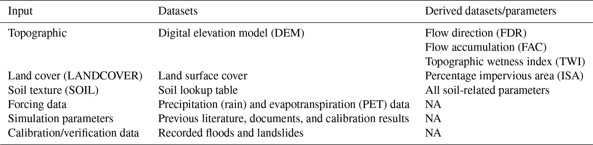
Table 1 Overview of inputs datasets needed in iHydroSlide3D v1.0.

NA: not available.

2.8 Model inputs and outputs

The model inputs can be summarized into four types (given in Table 1): meteorological forcing data, land surface feature data, simulation parameters, and calibration/verification data. The detailed description, value/resolution, and source can be found in Sect. 3. The abbreviations of input data correspond the file name in the simulating folders, helping users quickly identify and prepare necessary documents. The output variables include all typical hydrological components (e.g., overland runoff, soil moisture, and infiltration information) and landslide assessments (FSPFV_L and A_L). Note that model output is controlled by a user-defined global control file, and the components are thus selected based on the interest of the user. The model calls for two sets of topographic data (see Sect. 2.5), and all gridded data are either downscaled or aggregated to an objective spatial resolution to ensure the forcing and auxiliary data matching with each other. iHydroSlide3D v1.0 currently supports several different options for file formats (ASCII, TIFF, and TXT) and map projections, of which the Geographic Tagged Image File Format (GeoTIFF) is preferred for its distinct advantage of containing native compression capabilities, making the file sizes smaller.

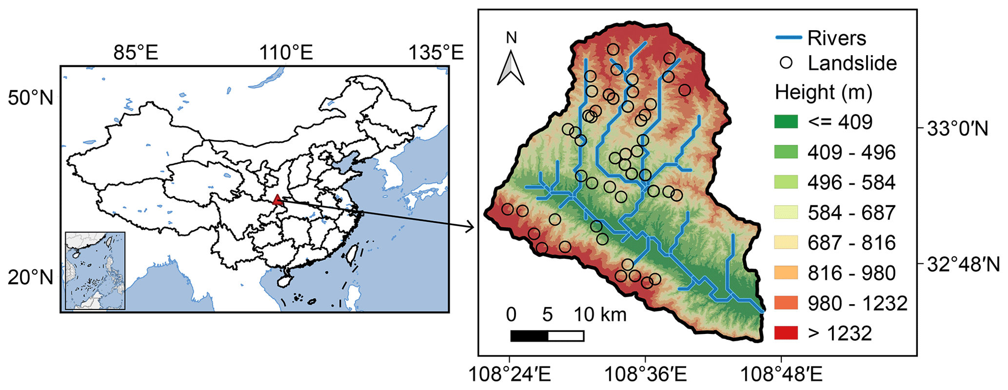
Figure 5 Locations of the Yuehe River basin with its elevation and the reported landslide events.

3 Materials and model setup

We test the iHydroSlide3D v1.0 code in the Yuehe River basin, Shaanxi Province, China (Fig. 5). The basin has an elevation between 270 and 2700 $\mathrm{m}\mathrm{a}.\mathrm{s}.\mathrm{l}.$ and covers a total area of 1100 km². The terrain in this basin is characterized by steep hills, gullies, and valleys, while its flood season is usually accompanied by heavy and frequent rainfall. As a result, this basin is highly susceptible to slope instability and sliding (Zhang et al., 2019; Wang et al., 2020). In this area, 54 slope failure locations were reported during a rainstorm from 3 to 4 July in 2012 (no more specific time record). In addition, the discharge of the flash flood was also observed at the outlet of the basin.

Table 2 Lookup table of key parameters for different soil types used in this study (refer to Wang et al., 2020; and Zhang et al., 2016).

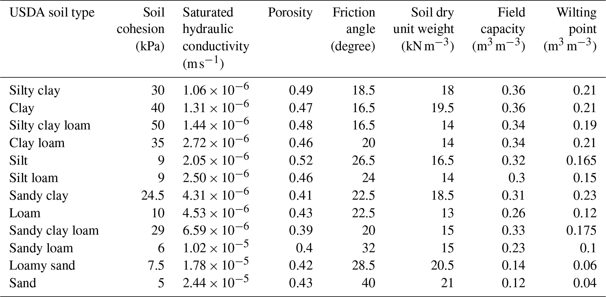
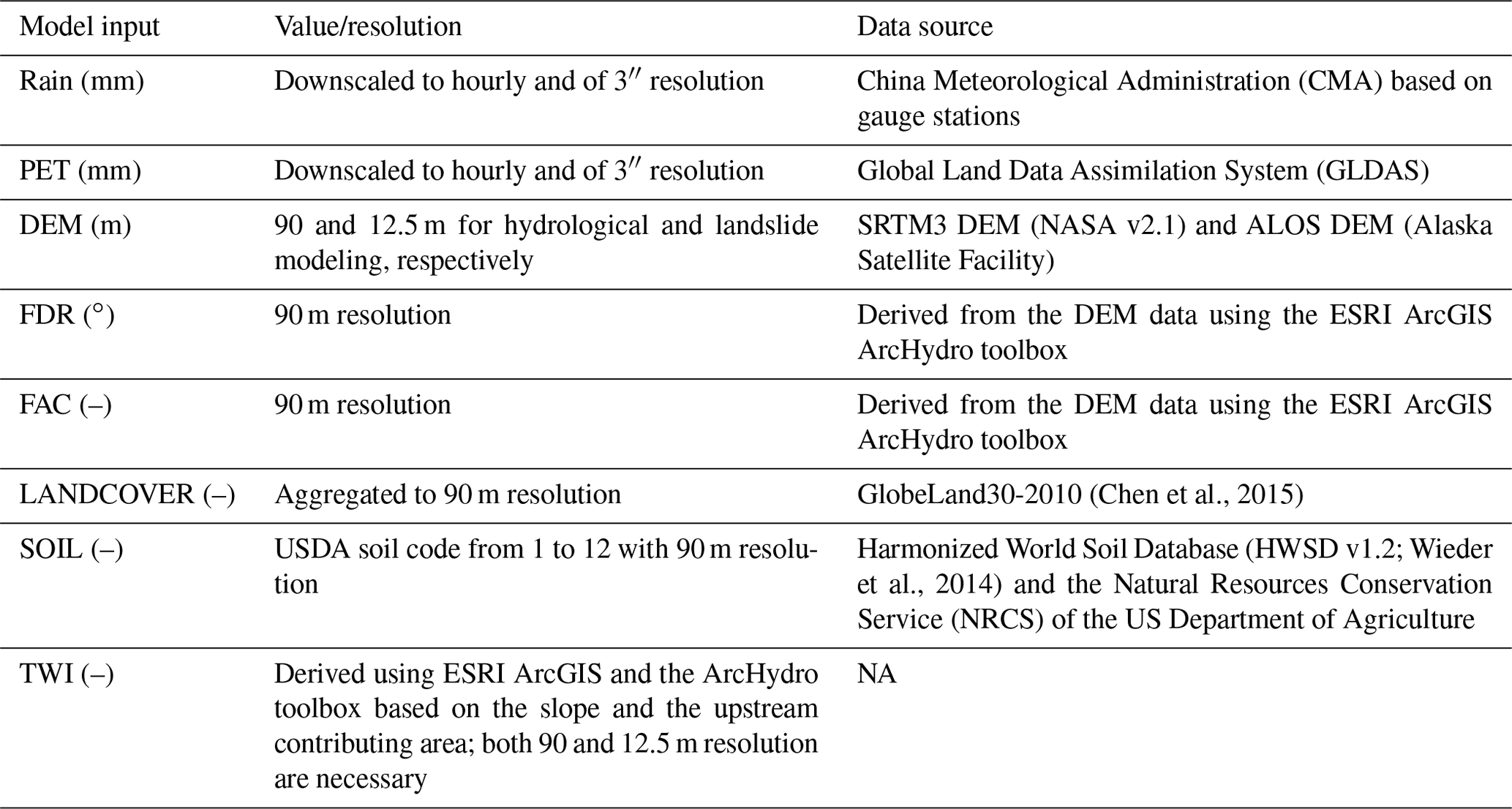
Hourly precipitation data were provided by the China Meteorological Administration (CMA) based on the observations of gauge stations and were interpolated into a spatial resolution of 3 arcsec (∼ 90 m). The potential evapotranspiration (PET) data were derived from the Global Land Data Assimilation System (GLDAS). The 3 h, 0.25^∘ PET data were first downscaled to a resolution of 3^′′ using bilinear interpolation and further downscaled to an hourly scale using linear interpolation. Two different resolutions of DEM (90 and 12.5 m) from the NASA Shuttle Radar Topography Mission (SRTM) version 3.0 (SRTM3) DEM and Advanced Land Observing Satellite (ALOS) DEM are used for hydrological and landslide modeling (introduced in Sect. 2.5), respectively. The flow direction (FDR) and flow accumulation maps (FAC) are necessary for hydrological simulation and can be derived from the DEM map. The slope angle map is optional for hydrological modeling but required for landslide modeling, which can be directly computed through a built-in slope angle calculation function in iHydroSlide3D v1.0. The TWI data were derived using the ESRI ArcGIS and its ArcHydro toolbox. The land cover data were derived from the 30 m GlobeLand30-2010 data (Chen et al., 2015). Soil texture was classified into the 12 United States Department of Agriculture (USDA) soil texture types from the Harmonized World Soil Database (HWSD v1.2) (Wieder et al., 2014) based on a lookup table (Table 2) shared by both hydrological and landslide modules.

Table 3 Detailed information of basic input data used in iHydroSlide3D v1.0.

NA: not available.

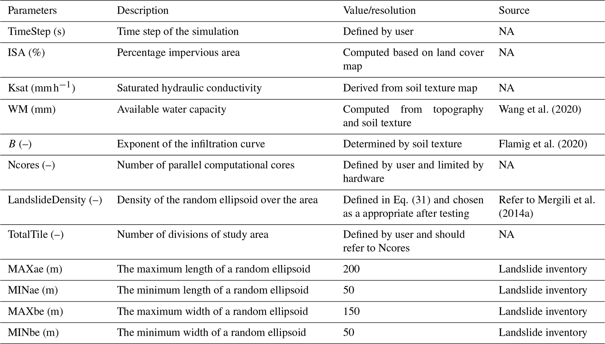
Table 4 Description of simulation parameters used in iHydroSlide3D v1.0.

NA: not available.

The parameters used for this model are largely related to an a priori map of soil information and have been generated by Wang et al. (2020) and Zhang et al. (2016). W_m corresponds to available water capacity between field capacity and wilting point (Table 2) and is distributed according to both topography and soil texture (Yao et al., 2012; Wang et al., 2020). Saturated hydraulic conductivity (k_s) strongly depends on the soil type and is determined through the pedotransfer lookup table (Table 2). Impervious surface area (ISA) can obviously affect the hydrological process such as infiltration and runoff generation and is calculated for each grid cell by considering the fractions of artificial surface and wetland in a land cover map. For the landslide module, the constraints of the random landslides are regarded as a priori parameters depending on the inventory. The inventory did not record the dimensional information (length and width) for all landslides, but it recorded a few of them, from which we picked the maximum and minimum values to comprise the constraints. Considering the random interval equals the spatial resolution, the constraint boundaries were rounded to the integer for further simplification. The total tiles divided from the entire area, along with the landslide density and user-defined number of cores, are summarized as related to parallel computational parameters. The basic materials and parameters are listed in Tables 3 and 4.

We run the model on the high-performance (HP) cluster with one manage node and eight computational nodes (Intel^® Xeon^® CPU E5-2660 v4 at 2.00 GHz). Each node is equipped with a CentOS system featuring 28 cores and 64 GB of RAM. Utilizing hyper-threading technology, it can effectively achieve a total of 56 threads.

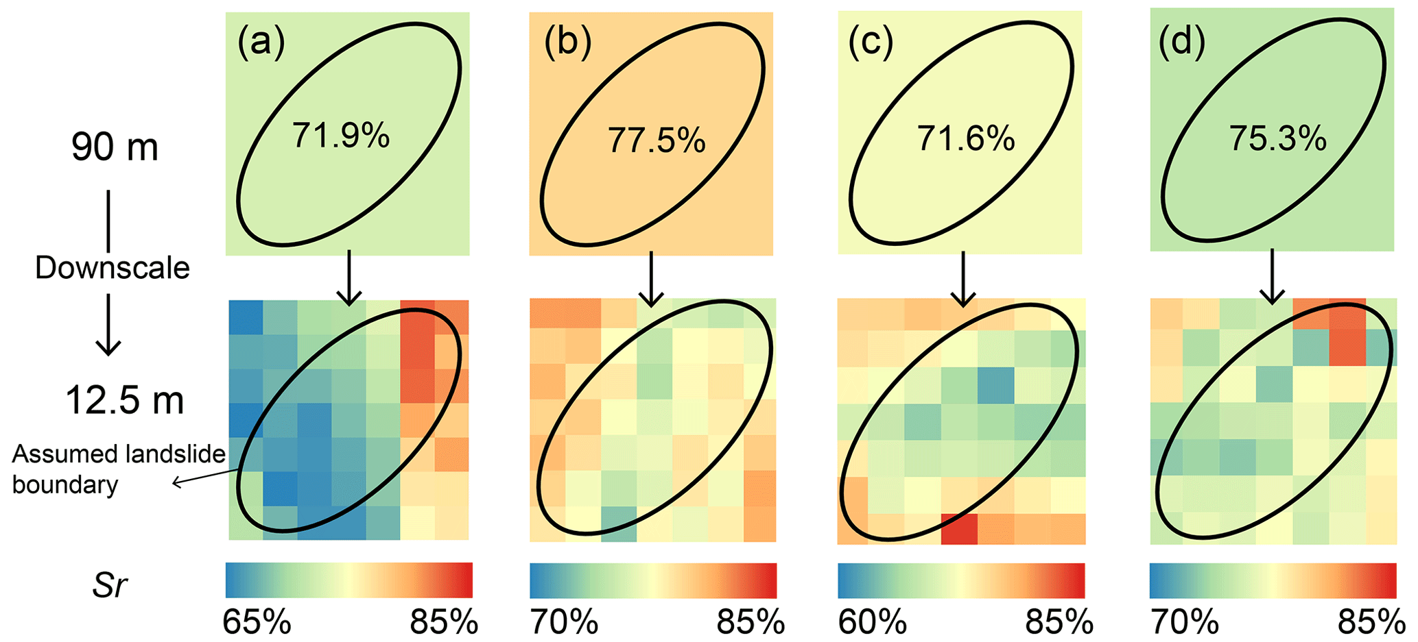
Figure 6 Soil moisture downscaling results from a coarser resolution (90 m) to a finer resolution (12.5 m). (a–d) Four grid cells selected from the 90 m resolution map. The ellipse is the assumed landslide boundary and encompasses the grid cells with the 12.5 m resolution.

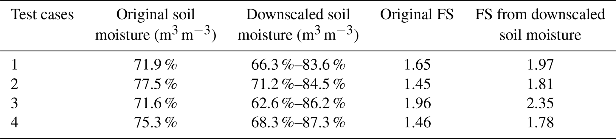
Table 5 Impacts of soil moisture downscaling on the potential slope failures in terms of the computed FS value.

4 Results

4.1 Evaluation of the soil moisture downscaling method

We first evaluated the impacts and effectiveness of the soil moisture downscaling method, which provides more detailed soil water information (groundwater) for landslide modeling and may directly impact the stability assessments. Compared to the infinite landslide model (Wang et al., 2020), the 3D model can fully consider the grid cells encompassed by an assumed landslide boundary (elliptical outline; see Fig. 6). The cells were chosen from the 90 m resolution datasets with different antecedent soil water amount, of which the single value was converted to a range among over the 7 × 7 map with a 12.5 m spatial resolution (Fig. 6). The long axis (a_e) of the tested ellipse reaches the diagonal of the square as far as possible to encompass more soil columns, and the potential depth of a failure is set to 2 m. The downscaled soil moisture values are irregularly distributed (Fig. 6) because they are contributed by several factors with local slope angle as the major one (Wang et al., 2020). As a consequence, the factor of safety was computed to a different value when using the single or composed soil moisture values for an assumed landslide (Table 5). In these four test sites, the risks are computed as the worse situations. However, in reality, such effects will be more uncertain due to the fact that the location and geometry of a landslide and associated hydrological conditions are all variable during the modeling. We argue that this downscaling method is necessary when we perform iHydroSlide3D v1.0 in a cross-scale manner.

4.2 Testing landslide density

The model requires an appropriate user-defined landslide density that is highly related to model computation efficiency. This value is determined to satisfy the convergence of the results over the study area and an acceptable level of the running time. Similar work has been done in previous research (Mergili et al., 2014b), and, equally important, here we further study the relationship between the tile size and random ellipsoid density required. We carried out the convergence tests for three different sizes of a divided tile: 20 × 20, 50 × 50, and 100 × 100 (number of grid cells). For each scenario, we increased the d_s (see Eq. 31) value and compared the spatial pattern with the previous d_s step. Two computational targets, the cumulative changed area over the entire region (∑changed  pixels  area) and cumulative changed FS multiplied by area (FSR×area), were used to evaluate the quantity of the convergence results (Mergili et al., 2014b). The former target is easier to converge; i.e., all pixels have been assigned a relatively invariant value of FS, while another target is strongly affected by the area of the tile (Fig. 7). In general, all the scenarios have similar convergence processes in term of ∑changed  pixels  area (d_s=500 in Fig. 7). FSR×area is more difficult to converge with the increase in the total area because this cumulative value is closely related the total number of the cells. We note that there exists no theoretical value of landslide density due to the fact that the generation of the potential landslide is totally random. Strictly speaking, d_s=∞ will be an optimum value; however, there will always be a trade-off between the quality and efficiency of the calculation. Further, the increase for overall quality of the prediction cannot be found with a larger adopted density when the ∑changed  pixels  area has converged, which in turn can significantly increase the computational burden (Mergili et al., 2014a). Besides, the density is mainly determined by constraints for the randomization of ellipsoid dimensions, for which the value would be set based on necessary tests if the model is applied to a new area. For the application in this study area, we consider d_s=500 a sufficiently reasonable approximation. The computing time for simulation is 55 432 s, with 328 s per time step.

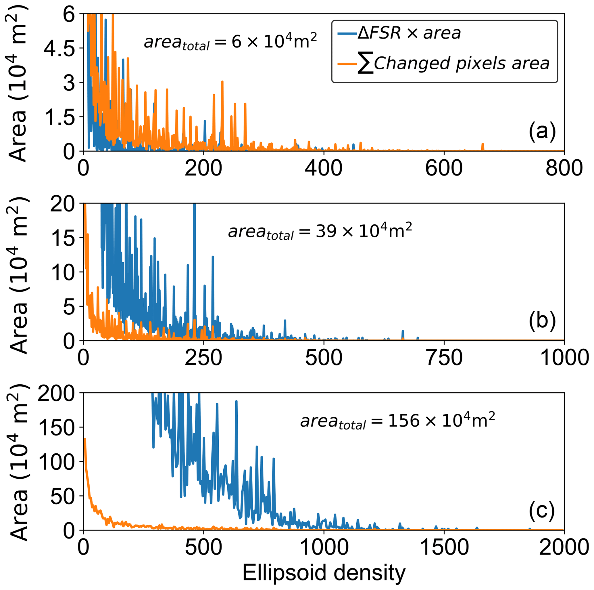
Figure 7 Landslide density tests for tiles with (a) 20 × 20, (b) 50 × 50, and (c) 100 × 100 grid cells. The total areas for the three scenarios are also presented. Two targets are computed during an interval of d_s=1.

4.3 Characteristics of rainfall and flood events

Provided the essential parameters and datasets are appropriately prepared for iHydroSlide3D v1.0, we choose 20 June, 00:00, to 15 July, 00:00 (UTC+08:00), as the simulation period, which is defined by two factors: (i) the period must include the main rainstorm triggering the flood and slope failures and (ii) the period should be longer than the observation period to exclude the effect of initial conditions (Zhang et al., 2016; Wang et al., 2020). As illustrated in Fig. 8, the rainstorm started around 4 July, 00:00 (UTC+08:00), reached the peak rate (exceeded 25 mm h⁻¹) within 5 h, and lasted for about a day across the region. The peak discharge was observed a few hours after the peak-rainfall moment, reaching a value close to 1000 m³ s⁻¹. The comparison between the modeled and observed discharge shows a generally good agreement with bias + 37.9 %, NSEC + 0.77, and CC + 0.93, respectively (Fig. 8). The slightly large bias implies there is likely some uncertainty in routing or flow concentration processes depicted by the hydrological module in iHydroSlide3D v1.0. Moreover, the model is sensitive to the rainfall data (before 4 July, 02:00, and after 7 July, 14:00, UTC+08:00). As a result, uncertainty in the rainfall data may contribute to the bias in the simulated streamflow. Nevertheless, the above results indicate that iHydroSlide3D v1.0 is generally capable of simulating the flood events and runoff processes when the model is calibrated.

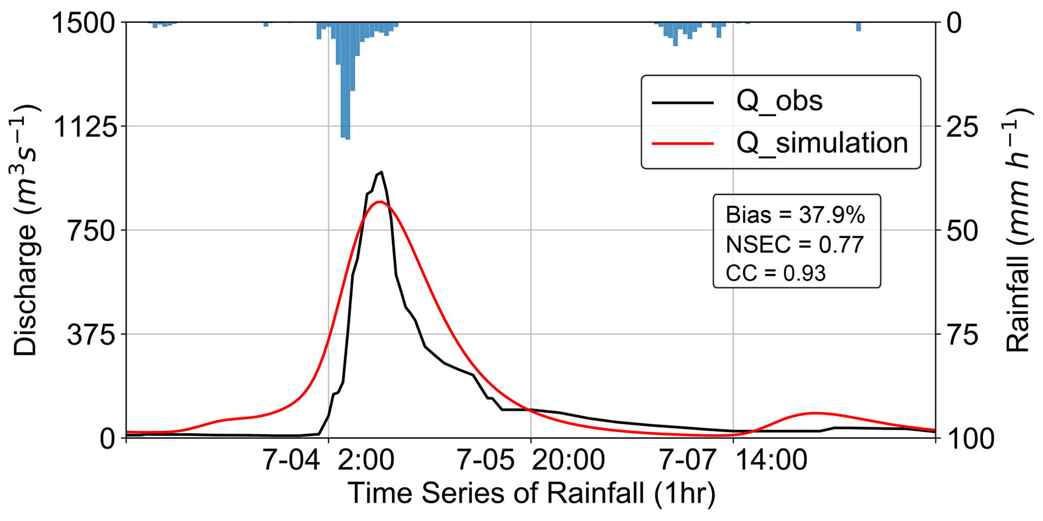
Figure 8 Basin-average rainfall rates and modeled hydrographs against the observed streamflow.

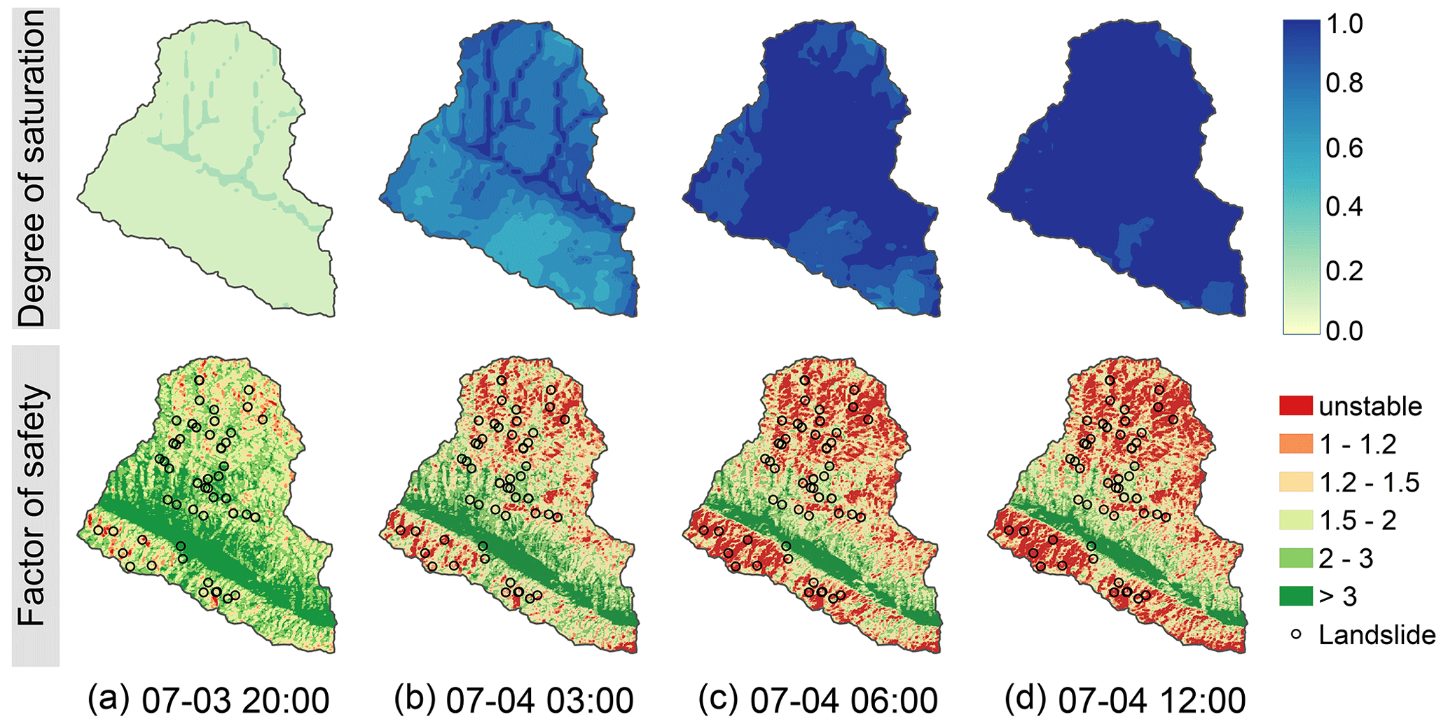
Figure 9 Spatiotemporal evolutions of the soil wetness (i.e., degree of saturation) and factor of safety. (a–d) Four moments that span the complete rainfall event.

4.4 Evolution of landslide risk responding to the hydrological process

4.4.1 Soil moisture and factor of safety

The evolutions of the soil moisture and landslide susceptibility are illustrated in Fig. 9. There is a small part of this region being predicted as unstable areas (Fig. 9a) in the beginning of the storm and can be explained by (i) the effect of antecedent rainfall or initial hydrological conditions and (ii) some grid cells that have steep slopes and are extremely unstable (Arnone et al., 2011; Aristizábal et al., 2016). These grid cells, generally located on very steep slopes, are more easily calculated as unstable areas in terms of FS value according to Eq. (19), which may bring some overestimation in iHydroSlide3D v1.0. However, we have attempted to avoid such weakness by using the wetting front concept with regard to slope failure depth (Eq. 26), which is subject to the hydrologic infiltration process and remains very small at the early stage of the rainfall event. As a result, a very small portion is estimated (Fig. 9a). The soil moisture drastically increases when the rainstorm starts, particularly for the computational elements (streaks in Fig. 9a and b) belonging to main routing channels of the drainage network. Based on the cell-to-cell flow routing rule, at the early stage of the storm, these cells have more chances to experience re-infiltration of excess surface runoff from upstream cells. As a consequence, they are more likely to reach a saturated condition. This phenomenon emphasizes the contribution of topography to the evolution of soil moisture at the early stage of a rainstorm, when the saturated hydraulic conductivity is relatively similar. In accordance with the soil moisture, more conditional unstable grid cells are predicted compared to the spatial pattern before rainfall starts. Soil moisture and landslide risk still continue to increase 3 h later and after the rainstorm reaches its peak; as a result, most of the study area is fully saturated, and unstable cells are substantially increased (Fig. 9c). Different from the early stage, the excess portion of rainfall cannot effectively be absorbed by soil anymore but contributes to runoff instead, leading to the flood along the river channel (Fig. 8). No significant difference can be observed between Fig. 9c and d, as the water amount of the rainfall has exceeded the infiltration demand and water capacity.

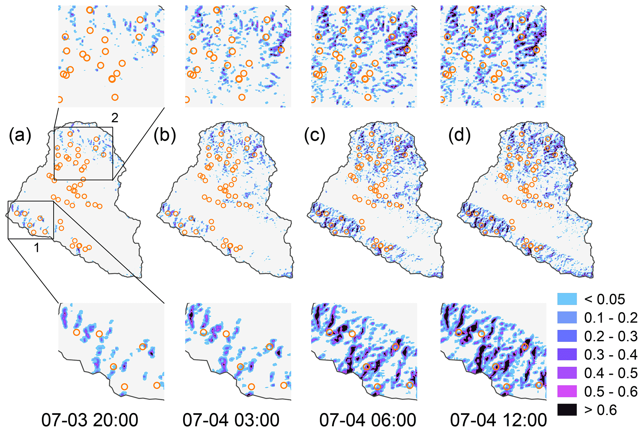
Figure 10 Spatiotemporal evolutions of the landslide occurrence probability. (a–d) Four moments that span the complete rainfall event.

4.4.2 Probability of failure

The model estimates the probability of failure for each grid cell due to the random operation of potential landslide generation (Sect. 2.7), although soil properties and hydrological conditions are deterministic. The original unstable areas were further re-classified to a different degree of probability (Fig. 10). We specifically divided the risk zones in terms of the PF values referring to the available classification (Lizárraga and Buscarnera, 2020; Vandromme et al., 2020): low (0 < PF < 5 %), moderate (5 % < PF < 30 %), high (30 % < PF < 60 %), and very high (PF > 60 %). As shown in Fig. 10a, most of the unconditional unstable areas fell in zones of low and moderate susceptibility whilst the others were estimated as the risks of high or very high. The former grid cells (e.g., inset 2 in Fig. 10), affected by the cell with a steep slope, might be computed as unstable because iHydroSlide3D v1.0 assesses the slope stability using the 3D landslide model (Eq. 19) and then outputs the minimum FS after random tests. In this work, relying on the PF classification, we can infer there are only a few steep grid cells (including themselves) near the grid cells with small values of PF – at least they are attenuated by the flat terrain. On the other side, for the grid cells with large PF values (e.g., inset 1 in Fig. 10, high or very high zones), the local topography is more likely to be continuous steep slopes that can be repeatedly calculated as unstable and thus cause larger PF values (Eq. 28). However, very few landslides are observed in the areas with steep slopes (Figs. 9 and 10). These areas may be covered by no or very thin colluvium or regolith; under this circumstance, soil depth tends to be negatively related to slope angle according to field survey or available soil-thickness models (Ho et al., 2012; Lanni et al., 2012; Alvioli and Baum, 2016; Tran et al., 2018). In this way, hazards like rockfall or avalanche are more expected instead of rainfall-induced landslides for these areas with extremely steep slope angles. Spatiotemporal evolution of the PF value shows that the probabilistic approach is capable of not only identifying the stable or unstable areas but also monitoring the unstable area in a more reliable and informative way. Compared to the binary assessment (stable and unstable), this method can help to better understand the relationship of landslide risk with local topography and dynamic hydrological conditions.

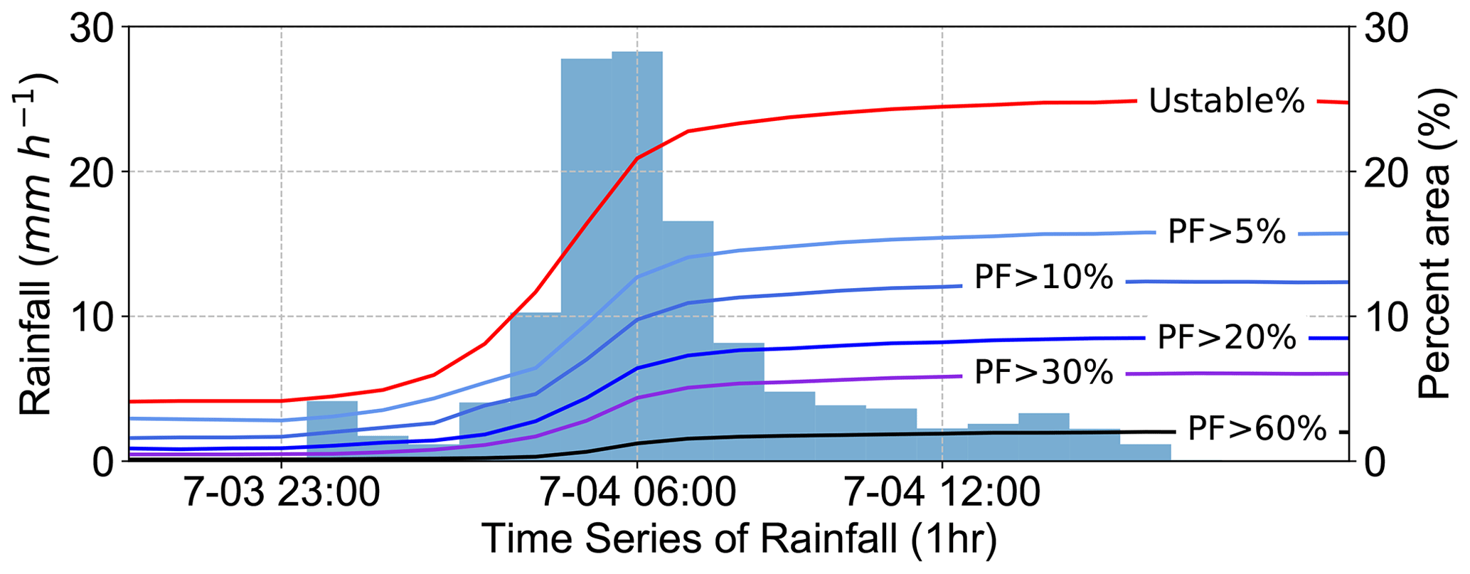
Figure 11 Evolution of percent area computed as unstable or various failure probabilities as the rainfall continues.

iHydroSlide3D v1.0 depicted the evolutions of unstable area and all risk zones (as percent of the whole region) introduced above over the computational time (curves in Fig. 11). These two areas are controlled by the patterns of FS and PF, respectively. Overall, the unstable area holds its leading position during the complete rainstorm. More specifically, FS values respond more dramatically to the rainfall event than PF values, which makes the unstable area increase more rapidly at the peak stage of the rainfall. This is not surprising because changing the value of PF should obey stricter rules (Eqs. 27 and 28) and experience repeatedly random tests. Among the various classes of the probability, the percent area and sensitivity to rainfall decrease with increasing PF-class value (see Fig. 11). At the early stage, the unconditional unstable area is computed to be less than 5 %, followed by other PF classifications with various thresholds. In particular, the percent area with PF > 60 % is close to zero – precisely 0.12 %. At the end of the rainfall (the soil is nearly fully saturated, and the curves are steady), the percent area with PF > 5 % is about 10 % less than the total unstable area, followed by the other zones of risk. A slight increase is observed for PF > 60 % (very high zone), with a significant contribution from the unconditional unstable areas. These areas could remain unaffected by the hydrological process (Aristizábal et al., 2016). The rest of the curves lie between them. The spatiotemporal classification of the landslide probability, as well as the traditional binary state of slope stability, is meaningful for landslide risk delineation and monitoring the area with a specific failure probability of interest.

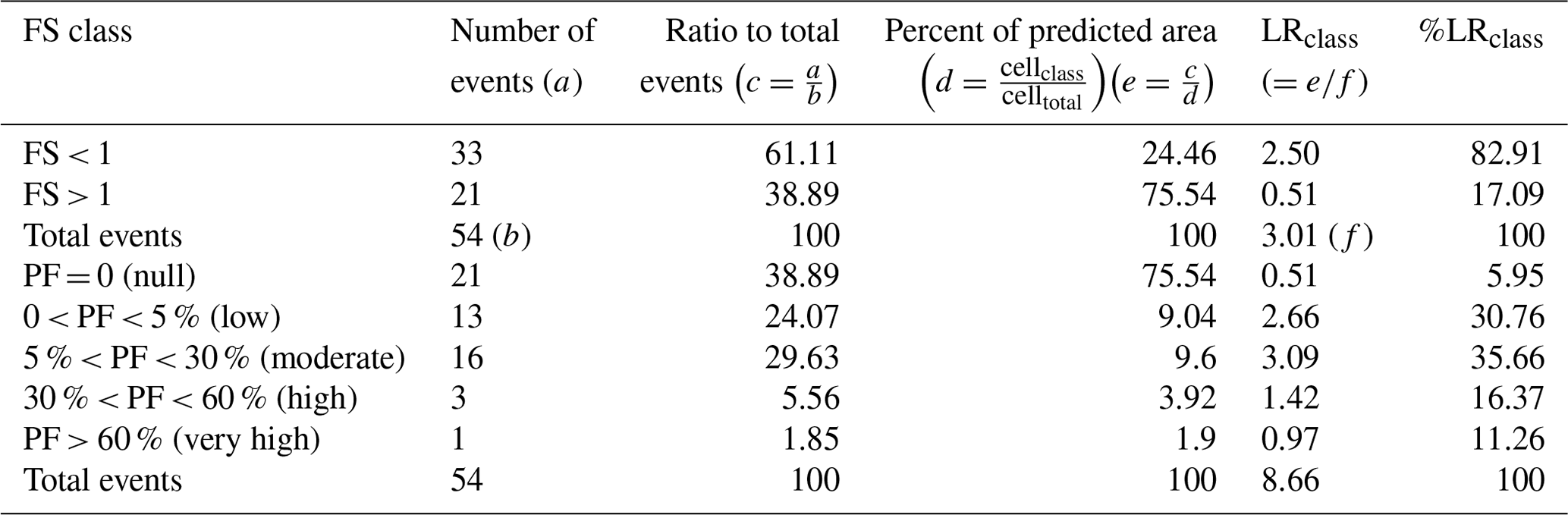
Table 6 Comparison of LR_class and %LR_class obtained from FS and PF values. The unstable areas are further divided into several risk zones with regard to their PF values.

4.4.3 Spatial performance of model

We evaluated the spatial performance of iHydroSlide3D v1.0 during the study period as presented in Table 6. We also compare our model with the previous coupled model CRESLIDE, of which the infinite slope stability is adopted (Fig. 12). Results show that 33 out of 54 landslides were successfully predicted, falling into the area with FS < 1 and PF > 0. For the zones of landslide risk, most of the failures (reaches 53.7 %) are observed in low and moderate risk zones, whilst the remainder are in the zones with high and very high risks. The value of the %LR_class index is evaluated as 82.91 % when using the factor of safety for prediction, and the same index reaches 94.05 % when we add up the values for all four risk zones. To be less conservative, the %LR_class index for PF prediction can be 82.79 %, which is close to the value by FS prediction, if we only consider the landslide risk from low to high. This result can be explained by the number of landslides per unit area; i.e., the binary approach would cover more extensive areas to contain the landslide locations. By adopting the probabilistic approach to identify classified risk zones, we can focus on the area of interest and make more targeted and efficient predictions.

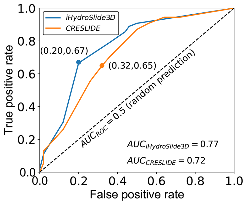
Figure 12 ROC plot comparing slope-stability results from the CRESLIDE model and iHydroSlide3D v1.0. The points on curves correspond to FS = 1 for both models. The AUC values are also shown in the plot.

The ROC analysis demonstrates that iHydroSlide3D v1.0 generally has a higher hit rate and lower false-positive rate relative to the CRESLIDE model that is coupled with the infinite landslide model. The area under the ROC curve (AUC) values for them are 0.77 and 0.72, respectively, suggesting that iHydroSlide3D v1.0 outperforms CRESLIDE in this case study. As mentioned in Sect. 2.3.2, the most significant difference between the two models is the assumption of landslide geometry. The 3D model takes the neighboring cells into account and thus provides a comprehensive FS value (Eq. 19), while the infinite models abruptly solve the limit equilibrium equation on a solo raster cell and are strongly conditioned by the local topography (Mergili et al., 2014b). This explains why the infinite-type models have a tendency to provide more conservative results (i.e., lower stability or worst situation) (Xie et al., 2006; Tran et al., 2018; Mergili et al., 2014b; Chakraborty and Goswami, 2016; He et al., 2021), indicated by higher false-positive rates (e.g., 0.32 for CRESLIDE versus 0.20 for iHydroSlide3D when the threshold equals 1) in this study.

Figure 13 Spatial patterns of the max values of (a) A_L and (b) V_L for model-predicted landslides.

4.4.4 Landslide hazard analysis

iHydroSlide3D v1.0 is capable of computing the extent (i.e., the area A_L and volume V_L) of potential landslides, which is essential for landslide hazard assessment. Compared to the visual techniques (e.g., aerial photograph interpretation and high-resolution imagery) or in situ investigation, the model estimates the A_L and V_L in a physics-based manner and strongly depends on the restrictions of random ellipsoids. In this way, A_L is simply determined by the number of encompassed raster cells, while V_L is computed by the soil columns and the failure depth associated with hydrological infiltration (Eq. 26). Therefore, there exist common phenomena that the values of V_L are more variable than that of the A_L; i.e., one unique A_L may correspond to multiple V_L values. Furthermore, it is possible for adjacent cells to share the same values of A_L and V_L, as they may fall within the same potential landslide. In this work, we recorded and presented the max value of the A_L and V_L as the worst scenario across the unstable area (see Fig. 13) after the sufficient random tests. Results show that most of the areas range from 4 × 10⁴ to 5 × 10⁴ m², while the volumes are more variable with a maximum value of around 1.1 million m³. The relatively large value of V_L may result from (i) a relatively large A_L that contains more soil columns or (ii) deep-seated landslides involved. It is worth noting that the areas with extremely large values of V_L (Fig. 13b) are roughly overlapped by the areas with relatively large PF (Fig. 10d). This can be explained by the fact that, in our pursuit of the minimum of the FS, a relatively thick failure depth was adopted in these areas, which caused an overprediction for landslide areas (Ho et al., 2012). Although the maximum magnitudes (A_L and V_L) of landslide hazards provide more conservative assessments, we expect that they are acceptable in slope engineering assessment (Tran et al., 2018).

Table 7 Relationships linking maximum landslide area A_L to landslide volume V_L.

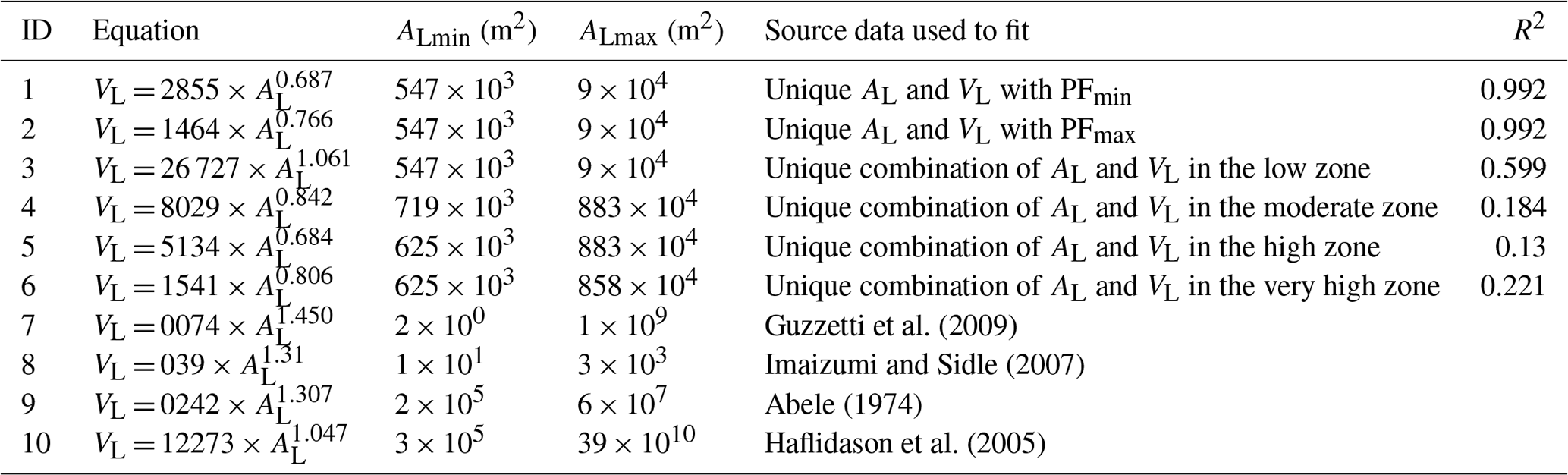
Column 1 lists the equation number. Column 2 shows the fitted equations in this work (ID 1 to 6) and available equations (ID 7 to 10) selected from previous literature. Columns 2 and 3 list the ranges of A_L applied for equations; the data for ID 1 to 6 are from this work; data for ID 7 to 10 are from the literature. Column 4 gives the data source. Column 5 lists the common statistical measure R squared (R²).

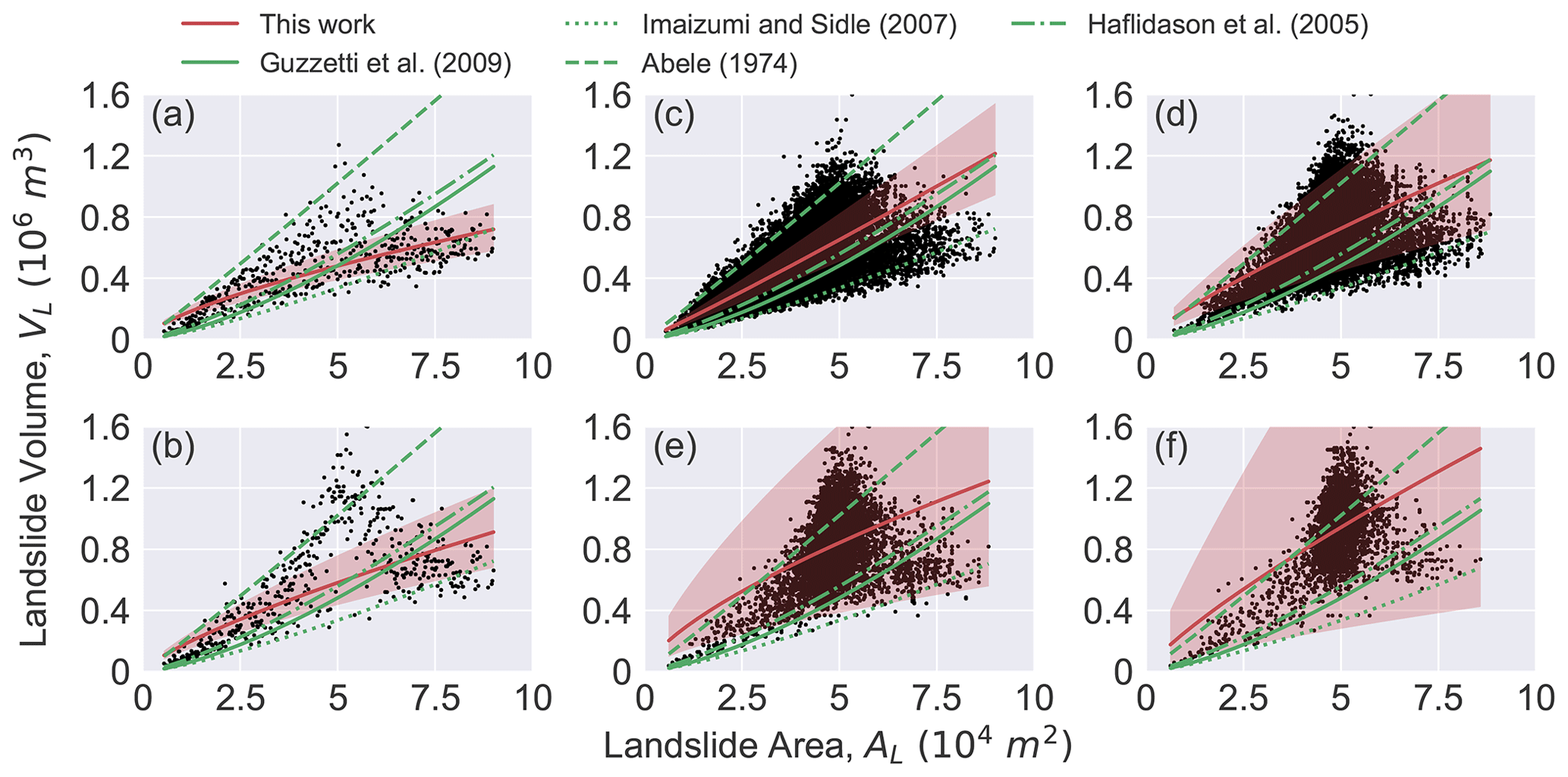
Figure 14 Six sets of source data (ID 1 to 6 in Table 7) are plotted and fitted in this work. All available equations (ID 7 to 10 in Table 7) are plotted by substituting the A_L values in this work. Red zone shows 95 % confidence intervals.

Due to a lack of historical documents for real A_L and V_L in this field, we evaluated the landslide hazard results by fitting the relationships of the A_L and V_L and comparing them with the existing relationships reported in previous literature. As the nature of these two geometrical properties introduced above, we did not collect all the values for each pixel. Instead, we prepared the fitted source into six datasets according to the combinations of A_L and V_L (source data in Table 7). All possible V_L values referred to the cases with PF_min and PF_max, as well as four risk zones. We further fitted these six sets using the power law and counted the R-square number (see Table 7). Moreover, as a comparison, we collected four available relationships from previous literature computed using field measurements in their study (Table 7, ID 7 to 10). We then plotted them by substituting the A_L values in this work (see Fig. 14). Obviously, relatively fewer data are plotted in Fig. 14a and b, which, as we have pointed above, shows all possible areas for potential landslides without a duplicate value. The values of V_L estimated with PF_max (Fig. 14b) are relatively larger than that with PF_min (Fig. 14a) because the deeper slip depth tends to obtain a smaller FS values, which in turn inevitably results in a larger volume of a failure. The fitted curves are close to the available equations in terms of trend, among which the Abele (1974) model overestimated the V_L in cases with ID 1 and 2. The efficiency of the fitted equations is generally good in terms of R², reaching 0.992. However, such a power model has low efficiency for cases of ID 3 to 6 with low R² and abnormally wide confidence intervals. Although these cases adopt the unique combinations of A_L and V_L, it is still very likely to accept the samples with identical A_L and consequently get more dots in the A_L∼V_L graph (Fig. 14c–f), which further limits fitting them as functions (i.e., a binary relation between two sets is defined as an association where each element of the first set is precisely linked to one element of the second set). In other words, they are regarded as a sampling error when the power model is considered. In this work, we can only provide relatively ideal geometrical information (with regular and limited characteristics) in a mathematical manner, which is determined by the cell size and random procedure. Even so, in the cases of ID 1 and 2, unique values of A_L are employed in the power models. Note that such relationships are not only limited to the maximum and minimum PF value but also any value of interest. For those applications limited by field measurements, the method proposed here is expected to roughly assess the magnitude of landslide hazards.

5 Discussion and conclusions

We have modified the 3D landslide model to make it applicable for more general situations (i.e., all possible soil moisture states). To this end, we incorporated the distributed hydrological model CREST to undertake the computational task of hydrological components, forming a new coupled hydrological–geotechnical model called iHydroSlide3D v1.0. The model is capable of assessing the spatiotemporal landslide susceptibility (FS and PF), performing hazard analysis (geometric properties of landslides, A_L and V_L), and predicting flash floods driven by rainfall processes. Considering differential needs for computational resolutions by the hydrological and landslide modules, we embedded the soil downscaling method to seamlessly execute the code within such a sophisticated framework containing two datasets with different resolutions. In addition, we parallelized the code of the landslide module for efficient large-scale performance. We evaluated our computational efficiency by comparing with two available parallel codes TRIGRS v2.1 (Alvioli and Baum, 2016) and r.slope.stability (Mergili et al., 2014a). The runtime for the single time step is 328 s for the present code, while it is 110 and 1900 s for TRIGRS v2.1 and r.slope.stability, respectively, in their descriptive literature. Such a comparison is unfair because the runtime was not obtained under the same testing prerequisites. Moreover, differences in model structure prevent them from being treated equally. TRIGRS v2.1 uses a simple infinite slope description, and r.slope.stability does not include the hydrological simulation. We show them here only for the general impression, upon which users may estimate the computational cost based on hardware and simulation scale.

Prior information on parameters is necessary for this model and needs to be handled with the utmost care. Most of the parameters are determined by available datasets and field records, while few of them are calibrated manually based on computational experimental tests. In particular, the landslide density could significantly affect the output results, and, even worse, a small value may yield meaningless results and unwanted consequences. Thus, the landslide density needs to be regularly tested when the code is applied for a new region. However, we would preliminarily recommend d_s=500 for a rough assessment as it has been tested in detail in this study and a study by Mergili et al. (2014a). We conclude that the converged density value tends to be irrelevant to the tile area once the constraints of the landslide's shape are determined. We also argue that the soil downscaling method is necessary when we run the hydrological and landslide modules at different resolutions, because the uneven soil moisture patterns exactly impact the slope-stability assessment. In particular, the 3D stability model should sufficiently consider the spatial distribution of soil moisture within an objective slip surface. This is a typical difference when we adopt the downscaling method compared to the infinite stability model (Wang et al., 2020).

In this work, we have prepared the observed river streamflow from the gauge and the point-like landslide locations. Although we have gotten a generally good agreement with the observations in terms of discharge and similar efforts have been made in previous studies (He et al., 2016; Zhang et al., 2016; Wang et al., 2020), the results cannot directly prove that the soil moisture is accurately estimated, which is truly associated with slope stability, per se. Other soil moisture data through site measurement (Lepore et al., 2013) or satellite (Zhuo et al., 2019a, b) can be used to further validate the model performance. However, field measurements are usually not available, and even many boreholes can only cover some of the many grid cells in a large-scale region (Marin et al., 2021), making the representativeness of ground observations questionable. The observation from the satellite is useful for soil moisture in shallow depth, hindering the application for landslide predictions at a deep depth (Zhuo et al., 2019a). Therefore, we consider the soil moisture as an intermediate hydrological component, of which the spatial pattern is simulated at each time step.

The model advantageously provides a spatiotemporal perspective for the evolution of hydrological processes, as well as the landslide assessments and hazards. Together with the random operation, the model can simultaneously assign the unstable grid cells with the factor of safety and failure probability. We expect such a combination of landslide assessment analysis is effective and more targeted. Moreover, temporal monitoring of the process evolution is useful for dynamic management of unstable areas subject to rainfall events. The overall performance of the model is generally satisfactory based on the statistical metrics of both hydrological (bias, NSEC, CC) and landslide aspects (%LR_classROC−AUC). We further recommend that the %LR_class index can be appropriately used to evaluate the landslides within various zones of risk determined by PF ranges. Note that we did not distinguish the unconditional stable and unstable grid cells beforehand, although they can inherently occur in the landslide models built upon the limit equilibrium principle (Aristizábal et al., 2016). However, iHydroSlide3D v1.0 defined the failure depth by adopting the wetting front concept that is subject to the infiltration process. The model, therefore, can better target the rainfall event and reasonably handles the hydrologic initial conditions. In addition, the results also indicate that the 3D landslide model can ameliorate the overprediction problem, known to be present in the infinite landslide models.

The comprehensive assessments (for both flood and landslide) possibly contribute to land management and disaster risk management with professional analysis. The landslide susceptibility and hazard zoning are able to manage landslide hazard in urban/rural areas by excluding development in higher hazard areas and requiring hydro-geotechnical assessment in the planning stage (Fell et al., 2008). The conception has been introduced across some countries such as France (Fell et al., 2008) and Switzerland (Leroi et al., 2005). A recent work corroborated existing hypotheses that urbanization increases landslide hazards (Johnston et al., 2021). Our model could be used as a tool to study the importance of considering interactions with urbanization when predicting landslide hazards under climate change scenarios. The current modular framework and flexibility of modeling setup also make it feasible to link with other numerical weather prediction models and real-time forcings. These complicated applications generally require extraordinary computing resources to support. The verification for landslide geometric output (volume and surface area) is still limited by the available measured data (e.g., landslide scars used in Arnone et al., 2011). Instead, we evaluated them with the fitted power-law equations, which, together with the available relationships in previous studies, are used as statistical tools for analysis of regional landslide magnitude. We have not unveiled the fundamental geotechnical mechanics of landslides in terms of 3D geometry of the sliding surface, which need be solved through field investigation. The present study employs the limit equilibrium method and iteration in a manner akin to Marchesini et al. (2009). Notably, we expanded upon previous research by conducting model simulations over a considerably larger spatial extent, thereby yielding more fine-grained findings.

Another limitation is the geotechnical parameters extracted from the available datasets. Determining their values in this way cannot consider geotechnical uncertainty due to inherent temporal and spatial variability of terrain materials (Hicks and Spencer, 2010; Griffiths et al., 2011; Mergili et al., 2014a). One way to overcome the problem is adopting the Monte Carlo approach, examples of which can be found in literature (Raia et al., 2014; Mergili et al., 2014a; Vandromme et al., 2020). Such embedded probabilistic method, no doubt, will considerably bring additional computational burden. In addition, we associate the failure depth with the infiltration process in this work, neglecting the spatial distribution of soil thickness in a terrain, which shall be a subject of future studies by supplying different soil-thickness assumptions.

In summary, a new hydrological–geotechnical model, iHydroSlide3D v1.0, coupling a distributed hydrological model (CREST) and a three-dimensional slope-stability model (3D landslide model), was described and tested in this study. The model is capable of simulating the spatiotemporal evolutions of hydrological components and landslide susceptibility and hazard. In order to coordinate the different resolution of datasets required for hydrological and landslide modules, the soil downscaling module is embedded to ensure that the code can be seamlessly executed. For efficiency, we program the code within a parallel framework and, together with the auxiliary efforts, make it possible to run in a large region. The model comprehensively presented the consequences of rainfall-triggered landslides at the watershed scale. With the evaluations from both hydrological and landslide aspects, we highlight the performance of iHydroSlide3D v1.0 on back analysis and the potential for predicting cascading flood–landslide disasters. The produced zones of risk and landslide geometric properties are valuable for disaster prevention and risk management. The modeling system presented in this work is also designed as a framework and has the potential to adopt other hydrological or land surface model (LSM) schemes and landslide models as alternatives. Moreover, iHydroSlide3D v1.0 can be further improved by optimizing geotechnical parameters and adopting other soil-thickness assumptions.