Enhanced ocean wave modeling by including effect of breaking under both deep- and shallow-water conditions

Accurate description of the wind energy input into ocean waves is crucial to ocean wave modeling and a physics-based consideration on the effect of wave breaking is absolutely necessary to obtain such an accurate description. This study evaluates the performance of an improved formula recently proposed by Xu and Yu (2020), who took into account not only the effect of breaking but also the effect of airflow separation on the leeside of steep wave crests in a reasonably consistent way. Numerical results are obtained through coupling an enhanced atmospheric wave boundary layer model with the ocean wave model WAVEWATCH III (v5.16). The coupled model has been extended to be valid in both deep and shallow waters. Duration-limited waves under controlled normal conditions and storm waves under practical hurricane conditions are studied in detail to verify the improved model. Both the representative wave parameters and the parameters characterizing the wave spectrum are discussed. It is shown that the improved source-term package for the wind energy input and the wave energy dissipation leads to more accurate results under all conditions. It performs evidently better than other standard source-term options of ST2, ST4 and ST6 embedded in WAVEWATCH III. It is also demonstrated that the improvement is particularly important for waves at their early development stage and waves in shallow waters.

1 Introduction

Accurate modeling of ocean waves depends straightforwardly on a correct formulation of the wind energy supply to the waves through the ocean surface as well as the wave energy dissipation within the ocean surface layer and eventually on a thorough understanding to the physics underlying these two dynamic processes. The wind energy input supports the generation and growth of ocean waves, while the wave energy dissipation always occurs owing not only to the viscous property of the fluid but also to the effects of turbulent mixing and multiphase interaction that take place in the boundary layer at both sides of the air–sea interface. In the past decades, a tremendous number of research efforts have been made to enhance our understanding of the phenomena of wind energy input into ocean waves and the dissipation of ocean surface waves due to various mechanisms (Janssen, 1989, 1991, 2004; Hasselmann et al., 1973; Snyder et al., 1981; Donelan et al., 2006; Babanin et al., 2007; Ardhuin et al., 2010; Rogers et al., 2012). However, a comprehensive integration of the accumulated knowledge, particularly that developed under extreme conditions in shallow waters, does not seem to have been satisfactorily achieved up to date.

Janssen (1989, 1991, 2004) proposed the most classical formula for the wind energy input based on the resonance theory of Miles (1957, 1965), in which the wind drag as a deterministic function of the roughness height of the ocean surface is a critical parameter. Hasselmann et al. (1973) obtained an expression for the wind energy input by solving the wave energy equation and then calibrating parameters with field data from the Joint North Sea Wave Project (JONSWAP). Snyder et al. (1981) and Donelan et al. (2006) conducted field experiments in the Bight of Abaca; the Bahamas; and at Lake George, Australia, and included more physics in their formula for the wind energy input. Badulin et al. (2007) and Zakharov et al. (2012, 2017) proposed a new method to establish a theory for the wind energy input by considering the weakly turbulent law for wind–wave growth. In spite of these important achievements, the wind energy input is still not yet satisfactorily formulated, basically due to complexity of the phenomenon as well as the physics underlying the phenomenon.

Researchers have found substantial differences between wind energy input through ocean surfaces with and without wave breaking (Banner and Melville, 1976). Data collected during the Australian Shallow Water Experiment (AUSWEX) field campaign at Lake George, Australia (Babanin et al., 2007), showed that under a severe breaking condition, the wind energy input will increase to about 2 times that under a relevant non-breaking condition. Although the important effects of wave breaking as well as short-wave dissipation on wind energy input have been well understood (Janssen, 1989, 1991; Makin and Kudryavtsev, 1999; Hasselmann et al., 1973; Babanin et al., 2007), it was only recently that Xu and Yu (2020) proposed a formula to effectively include these effects. Xu and Yu's (2020) formula takes into consideration both the breaking effect and the effect of airflow separation on the leeside of steep wave crests in a reasonably consistent way. Despite its physics-based nature, a further evaluation of its performance in practical and more complicated wind wave conditions, however, is still necessary.

It is generally believed that, among the total wind energy transferred into the ocean waves, a part is absorbed by the long-wave components to support wave growth, while an even larger part is received by the short-wave components and quickly dissipated due to fluid viscosity, wind shear on the ocean surface and the turbulence effect related to wave breaking (Csanady, 2001; Jones and Toba, 2001). Formulation of the wave dissipation, however, is very difficult, and the available suggestions in the literature are rather controversial (Cavaleri et al., 2007). The earliest wave dissipation model is known to be the probabilistic breaking model originally presented by Longuet-Higgins (1969) and then improved by Yuan et al. (1986). Hasselmann (1974) proposed the whitecap model based on a mathematical formulation of the negative work done by the downward whitecap pressure on the upward wave motion. Phillips (1985) and Donelan and Pierson (1987) proposed the quasi-saturation model by assuming a local equilibrium relationship among wind energy input, nonlinear transfer and wave dissipation. Polnikov (1993) preferred the turbulence dissipation model which relates the loss of wave energy to the dissipation of turbulence kinetic energy. In addition to the theoretical studies, a significant number of experimental investigations have also been carried out (Phillips et al., 2001; Melville and Matusov, 2002; Donelan, 2001; Hwang, 2005). Based on the data measured at Lake George, Australia, Babanin and Young (2005) established an empirical model in which the concept of cumulative effect is introduced so that the contribution of low-frequency wave motion to breaking of high-frequency waves can be taken into account. It may be necessary to point out that most of the experimental studies are supported only by limited data.

WAVEWATCH III (WWIII), a successful third-generation wave model, has been widely used for simulating ocean waves in both deep and shallow waters. With great effort made by scientists around the world (Ardhuin et al., 2010; Zieger et al., 2015), parameterizations of the source terms in WWIII have been well calibrated under various conditions to achieve satisfactory results for evolution of an ocean wave spectrum. Under severe wave conditions, however, their accuracy is often unsatisfactory and the wave energy is underestimated even with an optimal choice of the parameters (Cavaleri et al., 2020; Campos et al., 2018; Mentaschi et al., 2015). Meanwhile, researchers found that the directional wave spectrum has been sometimes very poorly simulated even when the significant wave parameters are accurately represented (Fan and Rogers, 2016). Stopa et al. (2016) believed that all wave models have difficulty in describing the directional spread of waves. Although modelers usually tend to attribute the numerical error to the inaccuracy of the wind data or topography data, we must admit that imperfection of the source-term parameterization, especially under severe wave conditions, is also one of the main reasons.

In this study, improved formulas for the wind energy input and the wave energy dissipation are embedded into WWIII v5.16, though it may also be applied to other ocean wave models. The enhanced atmospheric wave boundary layer model (AWBLM) (Xu and Yu, 2021) is also coupled to ensure a more accurate wind stress evaluation at high wind speed and in finite water depth. The performance of the improved formulas is evaluated under both idealized wind conditions and real extreme conditions. Attention is also paid to their differences in deep and shallow waters. The structure of the paper is arranged as follows. The improved formulation as well as the framework of the coupled AWBLM–WWIII model are described in Sect. 2. Model verification under controlled conditions is presented in Sect. 3, while model verification under extreme wind conditions is presented in Sect. 4. Section 5 is a summary of conclusions.

2 Model description

2.1 Coupled AWBLM–WWIII model

The ocean wave model WAVEWATCH III numerically solves the energy conservation equation for the wave action density spectrum (WW3DG, 2016):

$$\begin{array}{}\text{(1)}& {\displaystyle \frac{DN}{Dt}}={\displaystyle \frac{S}{\mathit{\omega }}},\text{(2)}& {\displaystyle }S=S_{\mathrm{in}}+S_{\mathrm{ds}}+S_{\mathrm{nl}},\end{array}$$

where N(ω,θ) is the wave action density spectrum, ω is the relative frequency and S is the source/sink term given by Eq. (2). In general, the source term S must represent three different mechanisms: the wind energy input into waves S_in, the wave energy dissipation S_ds and the nonlinear wave–wave interaction S_nl. Although S_in and S_ds represent different physical processes, they should be considered and calibrated interrelatedly since the net effect of these two sources rather than each of them can be more accurately measured on many occasions and it is the net effect that governs the growth/decay of the ocean waves. S_nl plays a key role in the evolution of wave spectrum shape and may, at least theoretically, be evaluated through correctly solving the nonlinear transfer integrals. Note that, in shallow waters, the wave energy dissipation must include those due to bottom friction and depth-induced breaking, denoted by S_dsf and S_dsb, respectively, in addition to that due to whitecaps, denoted by S_dsw, i.e., $S_{\mathrm{ds}}=S_{\mathrm{dsf}}+S_{\mathrm{dsb}}+S_{\mathrm{dsw}}$. It may also be worthwhile mentioning that an accurate evaluation of the nonlinear interaction effect is surprisingly difficult for the high-frequency wave components, particularly in shallow waters. Therefore, it is frequently suggested to apply a semi-empirical theory for evaluating S_nl, i.e., let $S_{\mathrm{nl}}=S_{\mathrm{nl}\mathrm{4}}+S_{\mathrm{nl}\mathrm{3}}$, where S_nl4 and S_nl3 are expressed as functions of the wave frequency as well as the wave direction and represent the quartet and triad wave interactions, which play dominant roles in deep and shallow waters, respectively.

In order to accurately simulate ocean waves under moderate to severe wind conditions, as well as from deep- to shallow-water conditions, an advanced atmospheric wave boundary layer model (AWBLM) must be coupled into WWIII for a dynamic evaluation of the wind stress. The AWBLM applicable for this purpose is well described in Xu and Yu (2021), which may take effects of both ocean surface state and water depth into consideration, and has certain advantages compared to a simple quadratic formula for the wind stress. In the coupled model, the source terms are treated in the following way. Quartet–wave interaction is computed with the standard discrete interaction approximation (DIA). Note that, though it may bring some uncertainty into the numerical results for nonlinear effects, the DIA method is still widely employed in practical applications due to its minimum requirement on the computational efforts (Liu et al., 2017; Stopa et al., 2016; Ardhuin et al., 2010). Triad–wave interaction is evaluated with the Lumped Triad Approximation model (Eldeberky, 1996). The bottom friction effect is described by the simple model of JONSWAP (Hasselmann et al., 1973). The Battjes and Janssen (1978) parameterization is employed to represent the effect of depth-induced breaking. The parameters included in all source terms except for those with special emphasis follow the default setting. The wind energy input and the wave energy dissipation are considered a package in this study. WWIII provides four options typical of this package, i.e., ST2, ST3, ST4 and ST6, among which ST3 and ST4 are based on the same formulation of Janssen (2004) for the wind energy input. Since ST4 has been frequently reported to have a better performance than ST3 (Stopa et al., 2016; Beyá et al., 2017; Liu et al., 2017), the ST3 option is neglected in this study. The standard options are carefully compared with the improved model proposed by the present authors (Xu and Yu, 2020).

2.2 Improved model of Xu and Yu (2020)

The wind energy input in the improved model of Xu and Yu (2020), hereafter referred as the ST-XY option, is expressed by

$$\begin{array}{}\text{(3)}& {\displaystyle }{S}_{\mathrm{in}}\left(k,\mathit{\theta }\right)={\displaystyle \frac{{\mathit{\rho }}_{\mathrm{a}}}{{\mathit{\rho }}_{\mathrm{w}}}}\mathit{\omega }{\mathit{\gamma }}_{\mathrm{g}}\left(k,\mathit{\theta }\right)E\left(k,\mathit{\theta }\right),\text{(4)}& {\displaystyle }{\mathit{\gamma }}_{\mathrm{g}}\left(k,\mathit{\theta }\right)=a\left[b_{\mathrm{T}}\mathit{\lambda }{G}^{\prime }+\left(\mathrm{1}-b_{\mathrm{T}}\right)G\right]W^{\mathrm{2}}\sqrt{B_{\mathrm{n}}},\text{(5)}& {\displaystyle }\begin{array}{rl}W& =max\left(\mathrm{0},{\displaystyle \frac{U_{\mathrm{10}}}{c_{\mathrm{p}}}}\cos \left(\mathit{\theta }-{\mathit{\theta }}_{\mathrm{a}}\right)-\mathrm{1}\right)\\ & +a_{\mathrm{0}}min\left(\mathrm{0},{\displaystyle \frac{U_{\mathrm{10}}}{c_{\mathrm{p}}}}\cos \left(\mathit{\theta }-{\mathit{\theta }}_{\mathrm{a}}\right)-\mathrm{1}\right),\end{array}\text{(6)}& {\displaystyle }{B}_{\mathrm{n}}\left(k\right)=A\left(k\right)\underset{\mathrm{0}}{\overset{\mathrm{2}\mathit{\pi }}{\int }}{k}^{\mathrm{3}}E\left(k,{\mathit{\theta }}^{\prime }\right)\mathrm{d}{\mathit{\theta }}^{\prime },\text{(7)}& {\displaystyle }{b}_{\mathrm{T}}\left(k\right)=\mathrm{89.5}{\left(\sqrt{B_{\mathrm{n}}\left(k\right)}-\mathrm{0.0223}\right)}^{\mathrm{2}},\text{(8)}& {\displaystyle }G=\mathrm{2.8}-\mathrm{1.0}\left\{\mathrm{1}+\tanh \left[\mathrm{10}\sqrt{B_{\mathrm{n}}}{\left({\displaystyle \frac{U_{\mathrm{10}}}{c_{\mathrm{p}}}}\cos \left(\mathit{\theta }-{\mathit{\theta }}_{\mathrm{a}}\right)-\mathrm{1}\right)}^{\mathrm{2}}-\mathrm{11}\right]\right\},\end{array}$$

where ρ_a is the density of air; ρ_w is the density of water; ω is radian frequency; k is the wavenumber, which is related to ω through the dispersion relation; θ is the wave direction; E(k,θ) is the directional wave energy spectrum; γ_g(k,θ) is the wave growth rate; c_p is the celerity of the wave with peak frequency; U₁₀ is the wind speed at the 10 m level above the ocean surface; and θ_a is the wind direction. Note that the basic form of Eq. (3) follows the conventional assumption that S_in is proportional to the directional wave spectrum. However, the most crucial factor in S_in, i.e., the wave growth rate γ_g, is formulated to represent the effect of various physical processes. Although γ_g is essentially governed by the relative wind speed and the mean steepness of the surface waves, it is considered to be essentially different when wave breaking does or does not occur and is thus expressed as a weighted average of the different multipliers corresponding to breaking and non-breaking conditions with the breaking probability b_T being the weight. The relative wind speed is expressed by Eq. (5), where deflection of the wind direction from the wave direction is fully considered. It may be necessary to point out that the contribution of the inverse wind to energy input is reduced by a factor of a₀=0.45 following Liu et al. (2017). Under the non-breaking condition, a separation coefficient G is introduced to represent the “shelter effect” due to airflow separation at the lee side of high wave crests following Donelan et al. (2006). When wave breaks, the “shelter effect” disappears and G reduces to its maximum value of $G^{\prime }=\mathrm{2.8}$. Since wave breaking has an effect of intensifying wind energy input, we introduce an amplification factor λ and let λ=2.0, also following previous studies. It may also be necessary to mention that the wave steepness is related to the saturated wave spectrum B_n(k), as expressed by Eq. (6), where A(k) is a measure of the directional spectrum width. In general, the wind energy input is positive, but it may become negative when a strong swell is present and the wind speed is smaller than the wave celerity or when the direction of wind is significantly deflected from the wave direction.

The advantage of the wind energy input in the improved model of Xu and Yu (2020) is its direct representation of the underlying physics. Based on the field observations of both Donelan et al. (2006) and Babanin et al. (2007), the wind energy input into waves under severe conditions is a very complicated process, since random waves may break and may not break depending on the instantaneous local wave steepness. For non-breaking waves, airflow separation occurs on the leeside of wave crests and the wind energy input reduces. For breaking waves, the wind energy input is significantly larger due to breaking-induced mixing. The improved model of Xu and Yu (2020) fully considers these two effects and, consequently, should be more suitable for the description of severe waves.

Since the ocean wave development actually depends on the net energy gain in the ocean surface layer and it is sometimes very difficult to identify if some amount of wind energy is transferred into the ocean waves and then dissipated or it is dissipated within the atmospheric boundary layer and not received by the ocean at all, S_in and S_ds must be considered a package. In other words, formulation of the dissipation term should be based on a relevant definition of the wind energy input. In this study, we follow the wave dissipation model of Ardhuin et al. (2010) for the whitecap effect. The semi-empirical dissipation model of Ardhuin et al. (2010) can be expressed as (see also Leckler et al., 2013)

$$\begin{array}{}\text{(9)}& {\displaystyle }{S}_{\mathrm{dsw}}=S_{\mathrm{dsn}}+S_{\mathrm{dsc}},\text{(10)}& {\displaystyle }\begin{array}{rl}{S}_{\mathrm{dsn}}& ={\mathit{\xi }}_{\mathrm{n}}{B}_{\mathrm{r}}^{-\mathrm{2}}\mathit{\omega }\left\{{\mathit{\delta }}_{\mathrm{d}}max{\left[B\left(k\right)-B_{\mathrm{r}},\mathrm{0}\right]}^{\mathrm{2}}+\left(\mathrm{1}-{\mathit{\delta }}_{\mathrm{d}}\right)\right.\\ & {\left.\max \left[B^{\prime \prime }\right]-B_{\mathrm{r}},\mathrm{0}\right\}}^{\mathrm{2}},\end{array}\text{(11)}& {\displaystyle }\begin{array}{rl}{S}_{\mathrm{dsc}}& =-\mathrm{1.44}{\mathit{\xi }}_{\mathrm{c}}\left\{\underset{\mathrm{0}}{\overset{r_{\mathrm{c}}k}{\int }}\underset{\mathrm{0}}{\overset{\mathrm{2}\mathit{\pi }}{\int }}max{\left[\sqrt{B\left(k^{\prime },{\mathit{\theta }}^{\prime }\right)}-\sqrt{B_{\mathrm{r}}},\mathrm{0}\right]}^{\mathrm{2}}\right.\\ & \left.\mathrm{\Delta }{c}_{\mathrm{p}}\mathrm{d}{\mathit{\theta }}^{\prime }\mathrm{d}{k}^{\prime }\right\}E\left(k,\mathit{\theta }\right),\end{array}\end{array}$$

where ξ_n and ξ_c are empirical constants, δ_d is a factor introduced to weight the isotropic part and direction-dependent part, and r_c is the minimum ratio of the wavenumber that will wipe out the short waves. The saturation spectrum B_n(k) is defined in the same way as before, and the directional saturation spectrum $B_{\mathrm{n}}^{\prime }\left(k,\mathit{\theta }\right)$ is defined by

$$\begin{array}{}\text{(12)}& B^{\prime }\left(k,\mathit{\theta }\right)={\int }_{\mathit{\theta }-{\mathrm{\Delta }}_{\mathit{\theta }}}^{\mathit{\theta }+{\mathrm{\Delta }}_{\mathit{\theta }}}{k}^{\mathrm{3}}{\cos }^{\mathrm{2}}\left(\mathit{\theta }-{\mathit{\theta }}^{\prime }\right)E\left(k,{\mathit{\theta }}^{\prime }\right)\mathrm{d}{\mathit{\theta }}^{\prime }.\end{array}$$

The threshold of B_n(k) is denoted by B_r. Note that Eqs. (9), (10) and (11) are based the assumption that wave dissipation consists of an inherent effect and a cumulative effect; both are proportional to the directional wave spectrum. In shallow waters, dissipations due to bottom friction and depth-induced breaking are formulated following Xu and Yu (2021).

2.3 Standard models

Known reliable formulas for the wind energy input and the wave energy dissipation have been embedded in WWIII. Among all of them, the following options, which have been widely preferred on different occasions, are chosen for comparison in this study.

1. ST2 option. This package, originally proposed by Tolman and Chalikov (1996), consists of the wind energy input formula of Chalikov and Belevich (1993) and Chalikov (1995) as well as a relevant wave energy dissipation model. The dissipation model emphasizes the different mechanisms of dissipation for low- and high-frequency waves. The expression for low-frequency waves is based on an analogy to energy dissipation due to turbulence, while that for high-frequency waves is purely empirical. A linear combination of these two expressions then represents the total dissipation. It has been reported that this wind energy input formula may need to be filtered using a special technique when a strong swell is present (Tolman, 2002). For the purpose of comparison, the default setting of parameters in this study follows Tolman (2002), who selected this package in WWIII for a global ocean wave modeling and obtained satisfactory results.

2. ST4 option. This package consists of the wind energy input formula of Janssen (2004), which is based on the wave growth theory of Miles (1957), and the wave energy dissipation model of Ardhuin et al. (2010). The dissipation model appears as the summation of an inherent part and a cumulative part. All parameters are determined following Ardhuin et al. (2010).

3. ST6 option. This package consists of the formulas for wind energy input and wave energy dissipation due to whitecaps which fit the field data obtained at Lake George, Australia (Donelan et al., 2006; Rogers et al., 2012). A sink term due to negative wind energy input is considered for inverse winds. The dissipation due to whitecaps is expressed as the sum of an inherent part, which is proportional to wave spectrum, and a cumulative part in terms of the integral properties of the wave spectrum below a certain value of the wavenumber.

3 Model verification under controlled normal conditions

3.1 Duration-limited waves in deep waters

The ideal problem of wave development over the open sea of infinite water depth is considered. At a given duration, evolution of the directional wave spectrum is simulated with WWIII considering different choices of the source-term package. The uniform wind speed at the 10 m height above the ocean surface is fixed at a moderate level of 10 m s⁻¹. Sensitivity of the numerical results to the computational time step is also studied. It is shown that a spatial resolution of $\mathrm{1}/\mathrm{30}{}^{\circ }$ is reasonably accurate for duration-limited wave simulations and a finer grid does not lead to any significant change in the numerical results. The boundary effect in the numerical results is minimized in this case by setting open boundary conditions surrounding a large-enough computational domain. It is also demonstrated that little difference in the numerical results can be observed as the computational time step takes 30 s, 1 min and 10 min. Therefore, the results obtained with the time step equal to 10 min are presented in the remaining part of this study.

In Fig. 1, the wave growth curve, i.e., the relationship between the normalized total wave energy ε and the normalized duration τ, computed with different options for the source terms, is presented and compared with the empirical results available in the literature. The four empirical growth curves correspond to Stewart's (1961) law, which was originally presented as tabulated data; Sanders' (1976) law; the CERC (1977) law; and Kahma and Calkoen's (1992) law. The equilibrium value given by the Pierson–Moskowitz spectrum (Pierson and Moskowitz, 1964), i.e., ${\mathit{\epsilon }}_{\mathrm{PM}}=\mathrm{3.6}\times {\mathrm{10}}^{-\mathrm{3}}$, and the tabulated values of Moskowitz (1964) are also plotted.

Figure 1 Comparisons of duration-limited growth rate between empirical and computational results. Both wave energy and duration are nondimensionalized with U₁₀.

By comparing the computed wave growth curves with each other and with the empirical results as well, it becomes clear that the WWIII model results with different choices of the source-term package are all rather close to the CERC (1977) law and Kahma and Calkoen's (1992) law and also agree with the results of Rogers et al. (2012). At a younger wave age, particularly at $\mathit{\tau }<\mathrm{2}\times {\mathrm{10}}^{\mathrm{3}}$, the ST-XY option performs much better, while other source-term options underestimate the wave energy significantly. The ST4 option most severely underestimates the wave energy at the early stage of wave development. As duration increases, the results of the ST6 option approach those of the ST-XY option. When approaching the equilibrium stage (${\mathrm{10}}^{\mathrm{4}}<\mathit{\tau }<{\mathrm{10}}^{\mathrm{5}}$), the numerical results corresponding to the ST-XY, ST6 and ST4 options all approach the Pierson–Moskowitz limit, while the ST2 option still underestimates the wave energy. In general, the performance of the ST-XY option is obviously better.

Since the source terms are often formulated in terms of the mean wave parameters, evolution of the wave spectrum and development of the mean wave parameters are thus interdependent. Therefore, a comparison of the mean wave parameters obtained with a different choice of the source-term options, as presented in Fig. 2, is highly meaningful. It is demonstrated that the significant wave height H_s and the mean wavelength L_m obtained with the ST-XY option are slightly greater than the results obtained with other options, while the ST2 option yields the smallest values. The numerical result of the mean wave period T₀₂ obtained with the ST-XY option is the largest at the early wave-development stage, but it becomes almost the same as that obtained with the ST4 option at the equilibrium stage. The mean wave period T₀₂ obtained with the ST2 option is the smallest at the early wave-development stage, while that obtained with the ST6 option becomes smallest at the equilibrium stage. The peak frequency f_p obtained with the ST4, ST6 and ST-XY options is very close to each other, but the ST2 option results in a larger value.

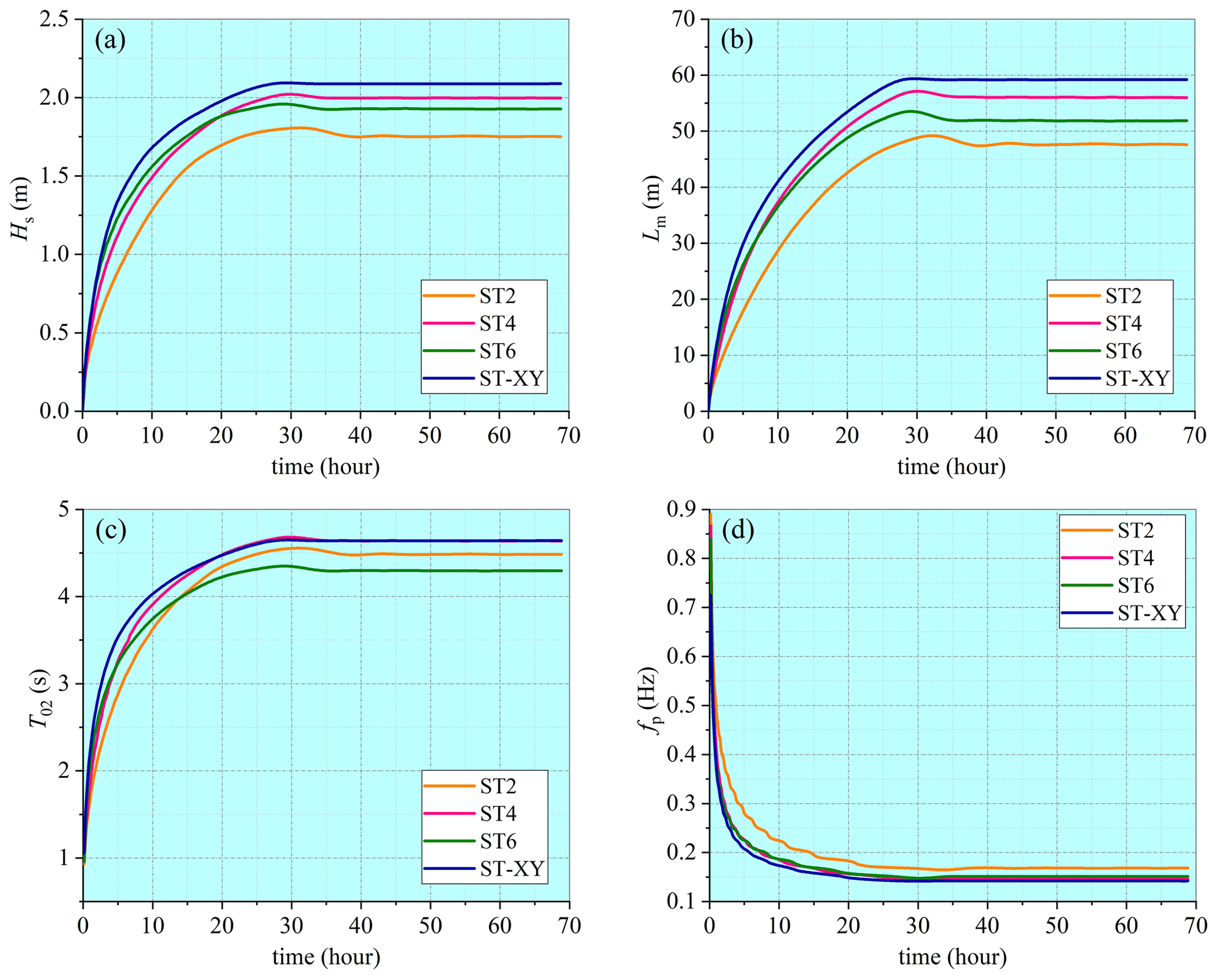
Figure 2 Comparisons of numerical results for (a) significant wave height H_s, (b) mean wavelength L_m, (c) mean wave period T₀₂ and (d) peak frequency f_p, obtained with different choices of the source-term options.

A comparison of the computed spectra of the wind energy input and the wave energy dissipation with different choices of the source-term options is presented in Fig. 3. Note that the spectra obtained with the ST2 option are not presented since they are obviously underestimated. The numerical results strongly indicate that the wind energy input and the wave energy dissipation resulting from the same source-term package are correlated, not only in terms of the peak values but also in terms of the spectral shapes. It is seen that the wind energy input resulting from the ST-XY option maintains a higher level than that resulting from other options at the early wave-development stage, leading to a faster wave growth and higher level of the wave energy at younger wave ages. Relatively concentrated unimodal distributions for both the wind energy input and the wave energy dissipation are built at the early wave-development stage, no matter which source-term option is adopted. As wave development continues, however, the peak frequencies as well as the peak values of the spectra decrease, while more wind energy is transferred to the higher-frequency waves and bimodal distributions are formed. At this stage, the peak value of the spectra obtained with the ST-XY option is similar to that obtained with the ST6 and ST4 option, while the high-frequency part has values higher than those resulting from the ST6 and ST4 options. When approaching the fully developed stage, the wind energy input obtained with the ST-XY and ST4 options reaches a peak at a relatively low frequency, but the peak obtained with the ST6 option appears at a much higher frequency. This is related to whether the breaking effect is fully considered when formulating the wind energy input.

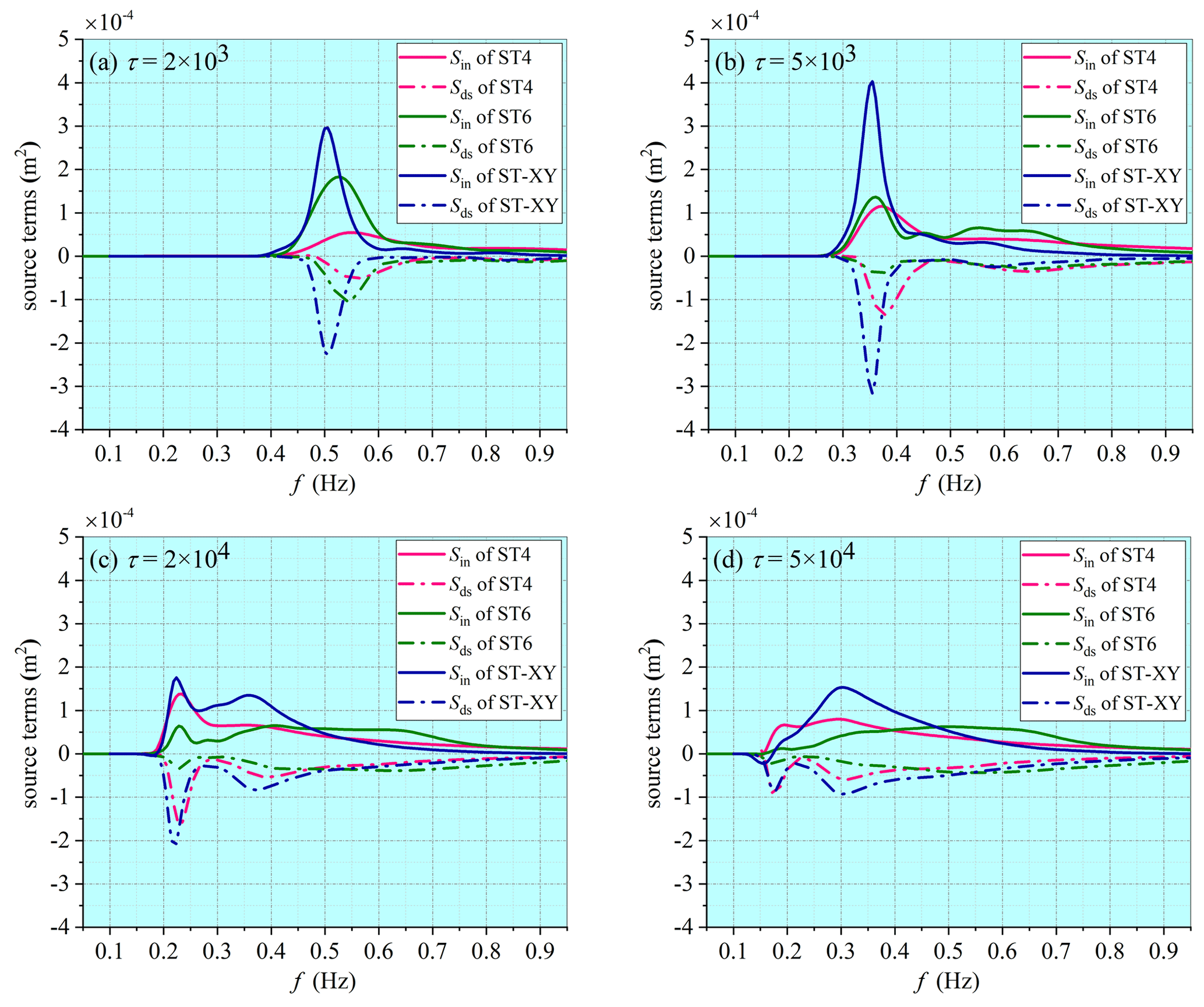
Figure 3 Spectra of the wind energy input and the wave energy dissipation obtained with different choices of the source-term package.

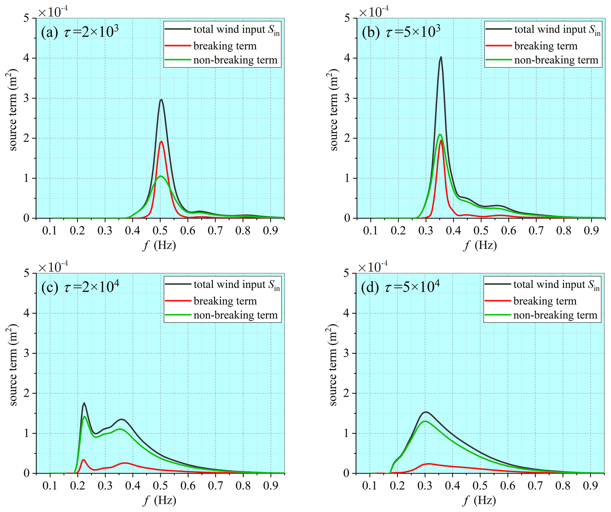
Figure 4 Deep-water spectra of wind energy input under breaking and non-breaking conditions at different wave-development stages given by the ST-XY source-term option.

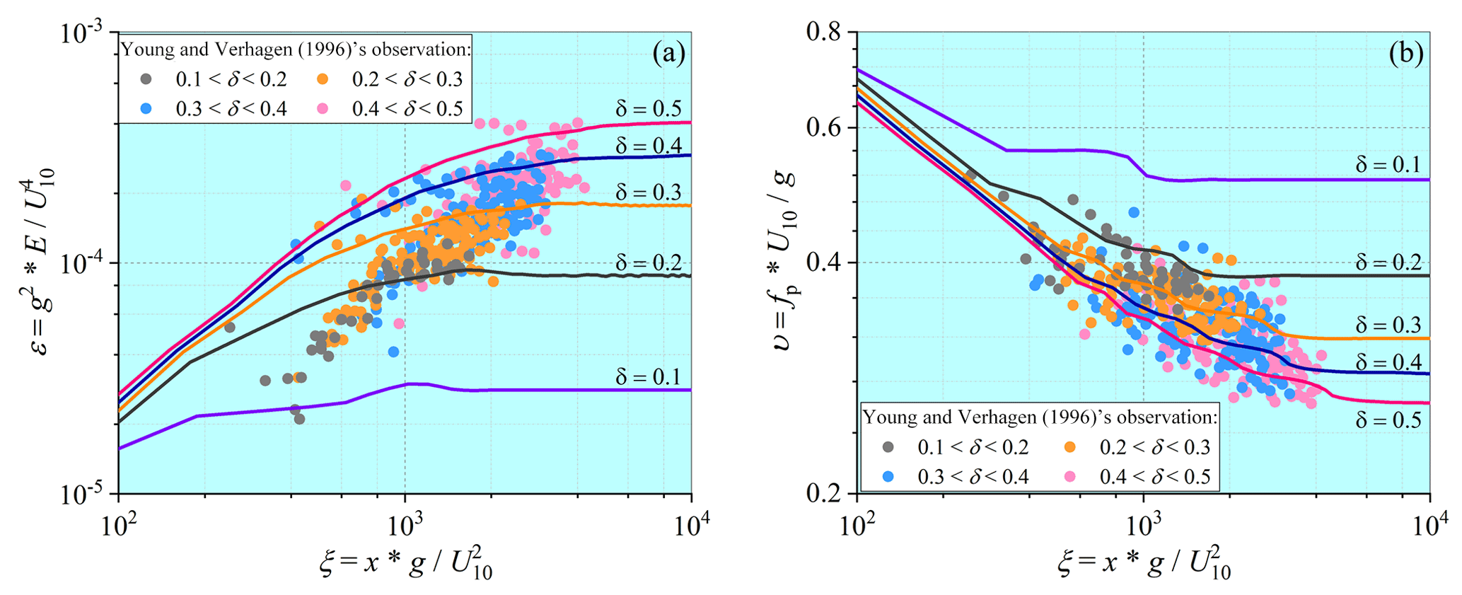
Figure 5 Comparisons of (a) fetch-limited growth rate and (b) wave age variation between measured and computed results.

A major merit of the improved formula for the wind energy input of Xu and Yu (2020) is the inclusion of breaking effect and the effect of airflow separation on the leesides of steep waves. Among the total wind energy input, the portions taking place under breaking and non-breaking conditions, given by the improved formula of Xu and Yu (2020), are presented in Fig. 4. It is clearly demonstrated that, at the early wave-development stage, over 60 % of the peak wind energy input takes place under the breaking condition. As wave development continues, the proportion of the peak wind energy input under breaking conditions decreases rapidly. When approaching the equilibrium stage, only 15 % of the peak wind energy input happens under breaking conditions. The trend suggested by our numerical results is in very good agreement with the facts reported in previous studies (Janssen, 1989; Hasselmann et al., 1973). Field observations indicate that wind energy input into breaking waves is about 2 times larger than that into non-breaking waves (Donelan et al., 2006; Babanin et al., 2007). Because of a relatively large amount of wind energy input into the breaking-wave components in the early wave-development stage, one observes a faster wave growth and higher level of the wave energy at younger wave ages. It is thus reasonable to conclude that the ST-XY option for the wind energy input and the wave energy dissipation successfully integrated the known information about the effect of breaking on the wind energy input and improved the performance of the WWIII model, especially at the early wave-development stage when the wave energy has often been underestimated.

3.2 Duration-limited waves in shallow waters

In order to evaluate its performance in the nearshore environment, the ST-XY source-term option is also applied to the simulation of duration-limited waves in shallow waters. The computational conditions are the same as those adopted in the deep-water case except for a varying water depth from 5 to 1 m. The nondimensional water depth $\mathit{\delta }=gd/U_{\mathrm{10}}^{\mathrm{2}}$ then varies from 0.5 to 0.1. The computational results are compared with field observations of Young and Verhagen (1996), who systematically measured the variations in wave parameters and wave spectrum in shallow waters. Since the measured data were provided in a fetch-limited manner, the method of Hwang and Wang (2004) is used to transfer the duration-limited numerical results to fetch-limited ones for comparison. As demonstrated in Fig. 5, the numerical results obtained with the ST-XY source-term option in shallow waters match well with the field data. As the nondimensional water depth increases from 0.1 to 0.5, the wave energy increases, while the peak frequency decreases. This is well explained by the effect of water depth on wave steepness and wave height. Within each range of the water depth, the field data basically fall into the relevant two curves resulting from the model. This is particularly accurate for the wave energy. Therefore, it may be concluded that the improved source-term option of Xu and Yu (2020) is also effective for ocean wave modeling under shallow-water conditions.

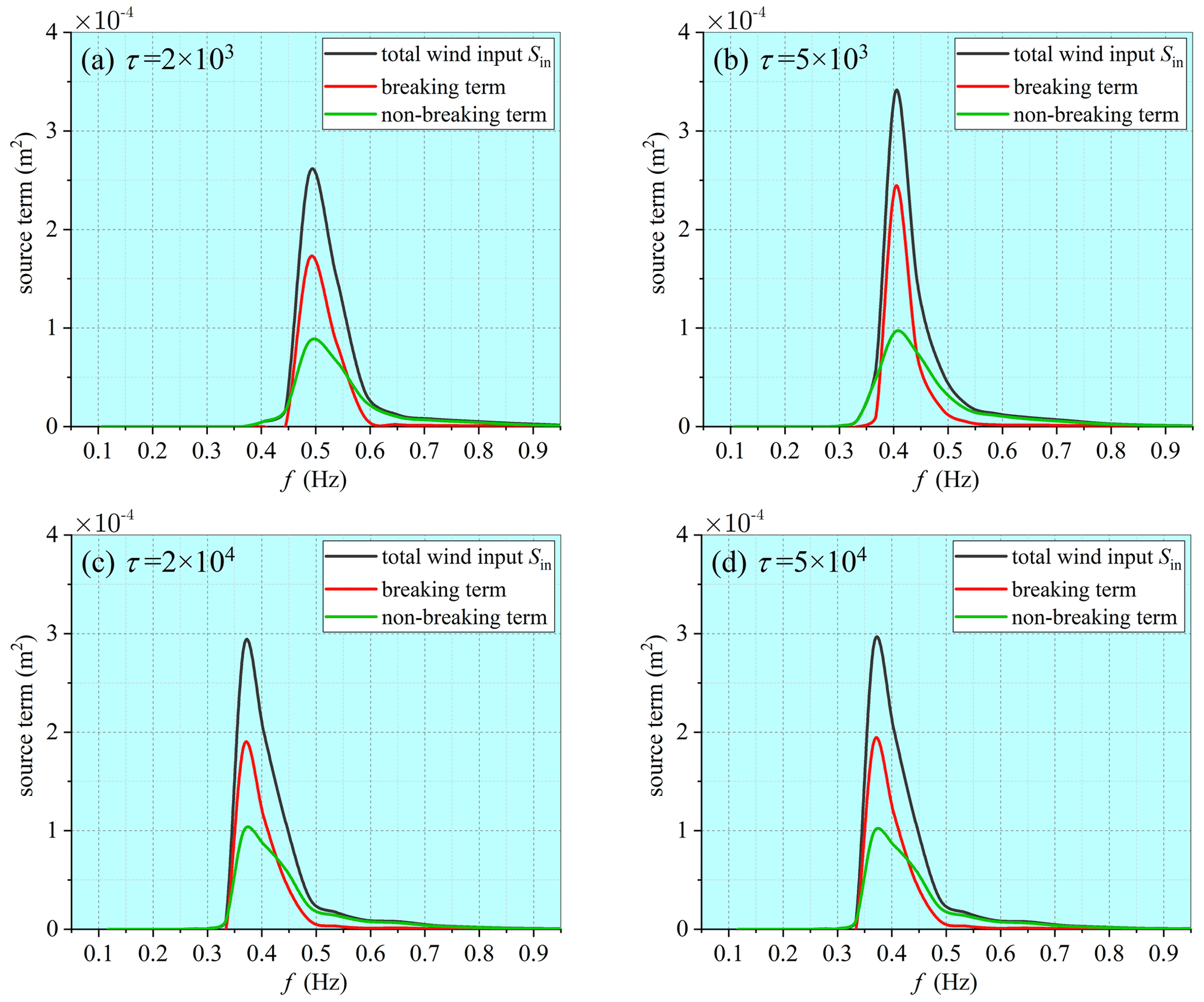
Figure 6 Spectra of wind energy input under breaking and non-breaking conditions resulted from the ST-XY source-term package at different wave-development stages in a water depth of 2 m.

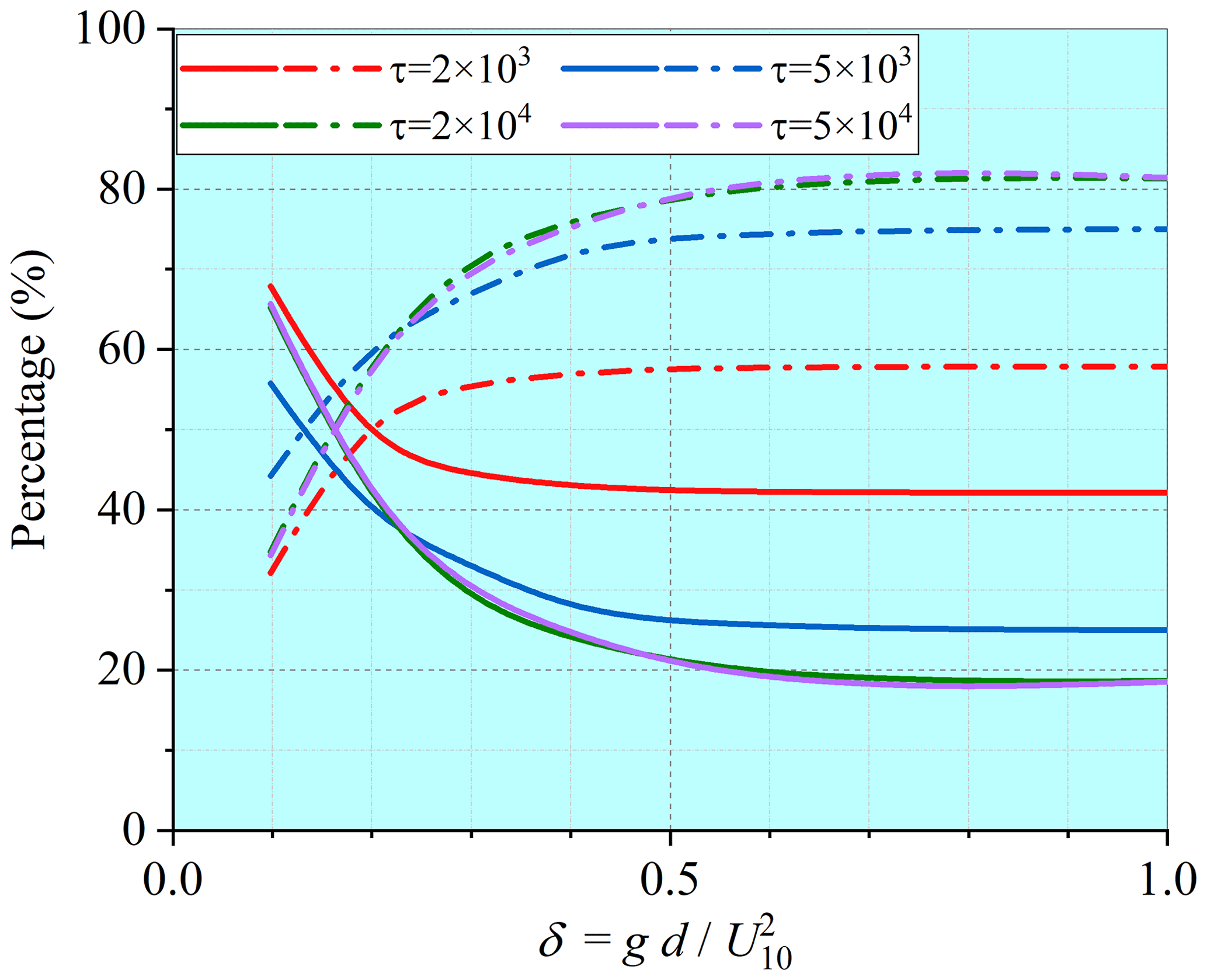
Figure 7 Variations in the percentage for wind energy input under breaking and non-breaking conditions. Solid lines are those under breaking conditions, while dot–dash lines are those under non-breaking conditions. Different colors stand for different wave ages.

Intensified breaking is a major feature of the shallow-water waves. Correct representation of the breaking effect in the wind energy input is thus very important for modeling shallow-water waves. Different from the deep-water situation, the peak value of the wind energy input taking place under breaking conditions is always higher than that under non-breaking conditions all through the early wave-development stage to the equilibrium stage, as presented in Fig. 6. The wind energy input taking place under breaking conditions remains a high proportion even at the equilibrium stage, indicating a more frequent breaking in shallow waters. In Fig. 7, the percentages of the wind energy input taking place under breaking and non-breaking conditions at different water depths and different stages of wave development are shown. At each wave-development stage, the percentage taking place under the breaking condition increases as the water depth decreases. At a given water depth, the breaking effect is more prominent at younger wave age but is still important at the equilibrium stage.

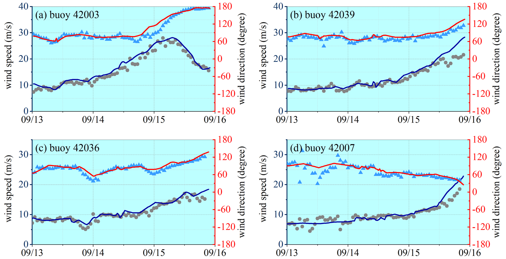
Figure 8 Comparison of reconstructed time series of wind velocity with observed data at locations of the National Data Buoy Center (NDBC) buoys during Hurricane Ivan. Scattered dots and triangles are buoy data of wind speed and wind direction, respectively. Blue and red lines are constructed wind speed and wind direction, respectively. Please note that the date format in this and following figures is month/day.

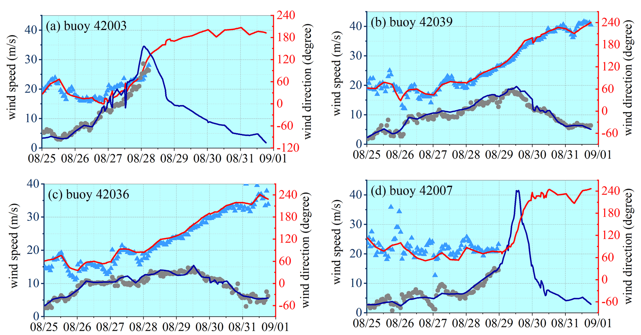
Figure 9 Comparison of reconstructed time series of wind velocity with observed data at locations of the NDBC buoys during Hurricane Katrina. Scattered dots and triangles are buoy data of wind speed and wind direction, respectively. Blue and red lines are constructed wind speed and wind direction, respectively. At buoy 42003 and 42007, there are data missing.

4 Model verification under practical extreme conditions

Storm waves under hurricane winds are characterized by the general young wave age and intensive breaking process, due to the extreme wind speed and rapid-changing wind directions. Therefore, their modeling requires an accurate description of the wind energy input to represent such characteristics. In this section, the effectiveness of the ST-XY source-term option is evaluated. Hurricane Ivan (2004) and Hurricane Katrina (2005), both of which made landfall on the coastline of the Gulf of Mexico, are chosen for our verification purpose. Hurricane Ivan and Hurricane Katrina are both typical, long-lived, category 4–5 tropical cyclones with well-recorded observational data. In fact, Hurricane Ivan and Hurricane Katrina have been extensively modeled and studied in the literature (Wang et al., 2005; Moon et al., 2008; Fan et al., 2009; Zieger et al., 2015). In addition, since the tracks of the two hurricanes lie in the same ocean basin, data of the topography, the forced wind and the ocean currents can be obtained from the same source, and the model settings can also be kept the same.

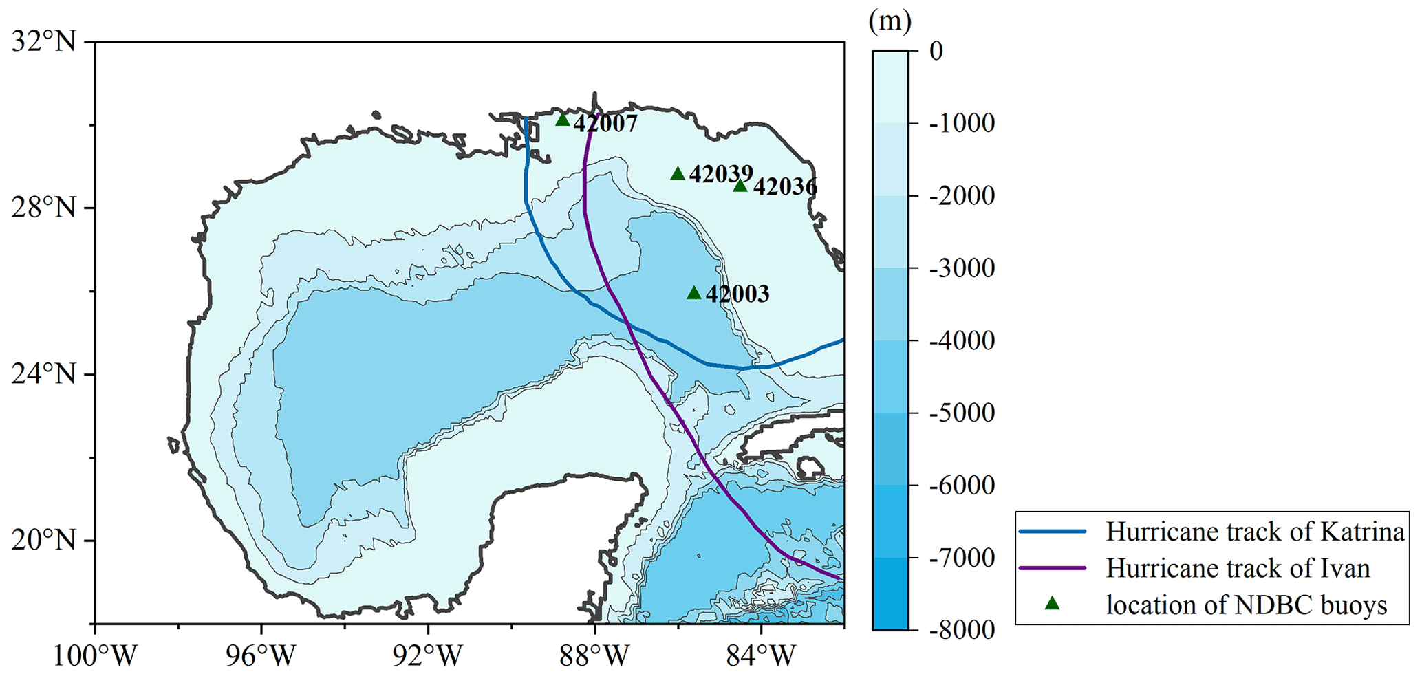
Figure 10 The computational domain. Tracks of hurricanes are shown with solid lines. The NDBC buoys are marked by triangles. Water depth at the locations of buoys 42003, 42039, 42036 and 42007 are 3265, 281, 50.9 and 14.9 m, respectively.

Table 1 Simulation errors in wave parameters during Hurricane Ivan.

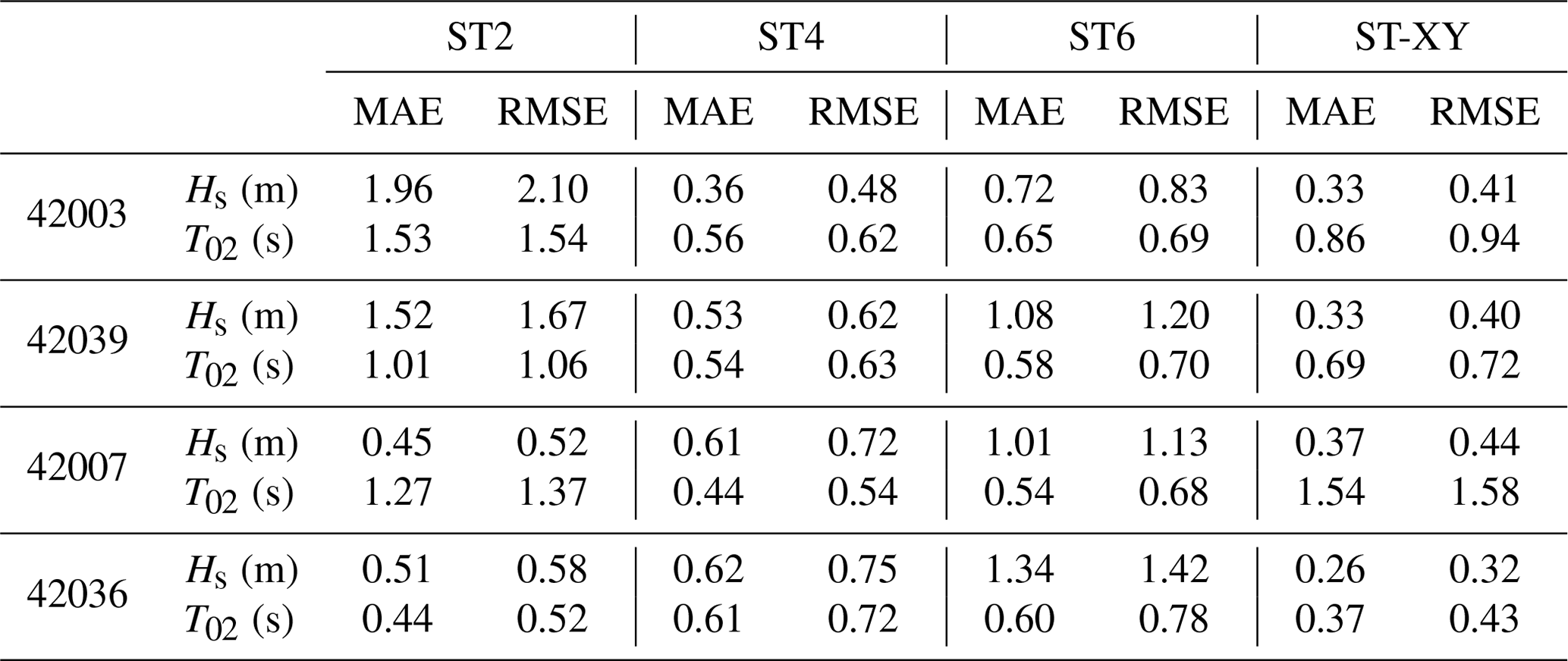
Figure 11 Comparisons of the computed variations (lines) of (a)–(d) H_s and (e)–(h) T₀₂ with buoy data (dots) during Hurricane Ivan.

4.1 Available data

It is very natural to require possibly the most accurate wind data for reliable model results on ocean wave development (Campos et al., 2018). In this study, we blend the H*Wind data (resulting from the Real-time Hurricane Wind Analysis System operated by the Hurricane Research Division of the National Oceanic and Atmospheric Administration) with the ECMWF (European Centre for Medium-Range Weather Forecasts) data to build the necessary wind field. The H*Wind dataset integrates all field data available during a hurricane event and is usually considered to be highly accurate in a certain range affected by the relevant hurricane (Fan et al., 2009; Liu et al., 2017; Chen and Yu, 2017). The H*Wind data are issued every 3 h with a grid resolution of 6 km and a spatial extent of $\mathrm{8}{}^{\circ }\times \mathrm{8}{}^{\circ }$ around the hurricane center. Because the H*Wind data do not cover the entire simulation domain, the ECMWF data must be supplemented. The ECMWF data have a spatial resolution of 0.125^∘ and temporal resolution of 6 h, which is good enough to represent the background wind field. The wind data from different sources are combined by setting a transition zone so that

$$\begin{array}{}\text{(13)}& {\mathit{U}}_{\mathrm{10}}=\left\{\begin{array}{ll}{\mathit{U}}_{\mathrm{H}}& \left(r<R_{max}\right)\\ \frac{R_{max}-r}{\mathrm{0.3}{R}_{max}}{\mathit{U}}_{\mathrm{H}}+\frac{r-\mathrm{0.7}{R}_{max}}{\mathrm{0.3}{R}_{max}}{\mathit{U}}_{\mathrm{E}}& \left(\mathrm{0.7}{R}_{max}<r<R_{max}\right)\\ {\mathit{U}}_{\mathrm{E}}& \left(r>R_{max}\right)\end{array}\right.,\end{array}$$

where U_H and U_E denote the wind velocity vectors from the H*Wind dataset and the ECMWF dataset, respectively; r is the distance from the hurricane center; and R_max is the maximal distance of the H*Wind boundary to the hurricane center. The time interval of the wind field is interpolated to 0.5 h to satisfy the computational condition. The normalized interpolation method of Fan et al. (2009), which ensures the greatest likelihood that the structure of the hurricane wind field is not affected by the interpolation, is applied for this purpose. The wind field constructed in such a manner agrees well with the buoy data as shown in Figs. 8 and 9. To include the effect of ocean currents (Fan et al., 2009), the global reanalysis database generated with HYCOM (HYbrid Coordinate Ocean Model) and NCODA (Navy Coupled Ocean Data Assimilation) is also utilized as the model input. The data have a spatial resolution of $\mathrm{1}/\mathrm{12}{}^{\circ }$ and a temporal resolution of 3 h. The topography data are from the ETOPO1 datasets and have a spatial resolution of 1^′.

Buoy data published by the NDBC (National Data Buoy Center, National Oceanic and Atmospheric Administration) are used to validate the model results on representative wave parameters including H_s, T₀₂ and spectral wave parameters in both deep and shallow waters. The locations of buoys are shown in Fig. 10.

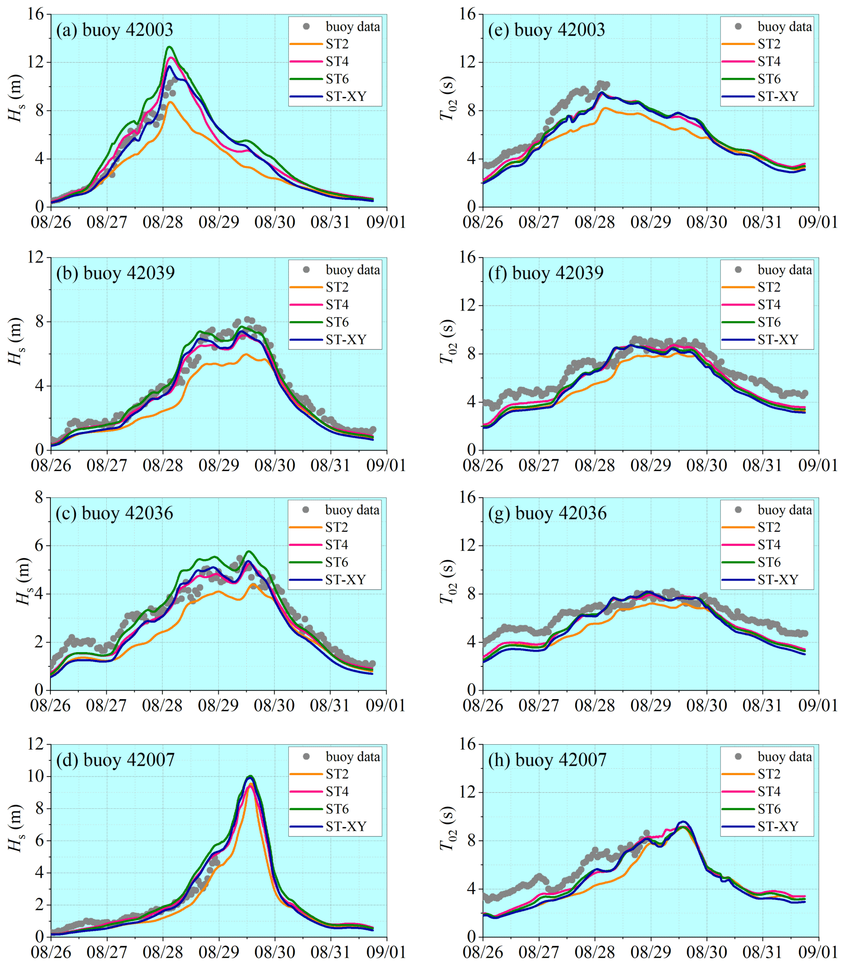
Figure 12 Comparisons of the computed variations (lines) of (a)–(d) H_s and (e)–(h) T₀₂ with buoy data (dots) during Hurricane Katrina.

Table 2 Simulation errors in wave parameters during Hurricane Katrina.

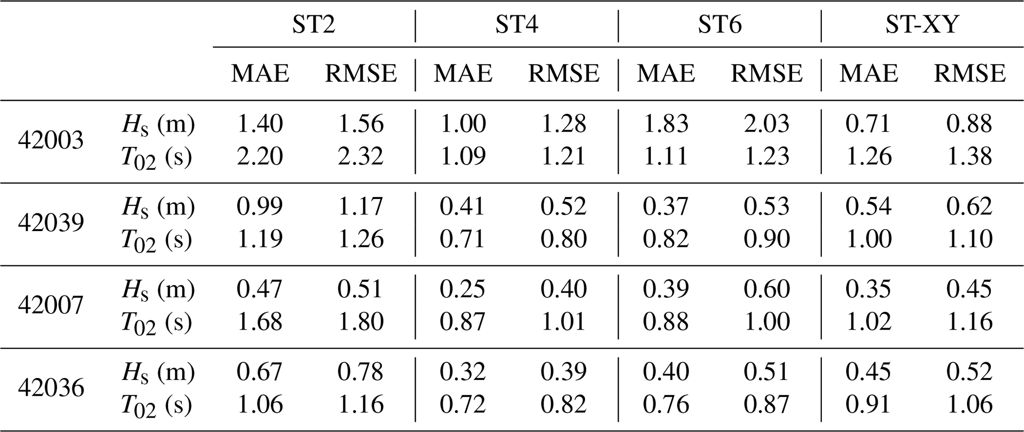
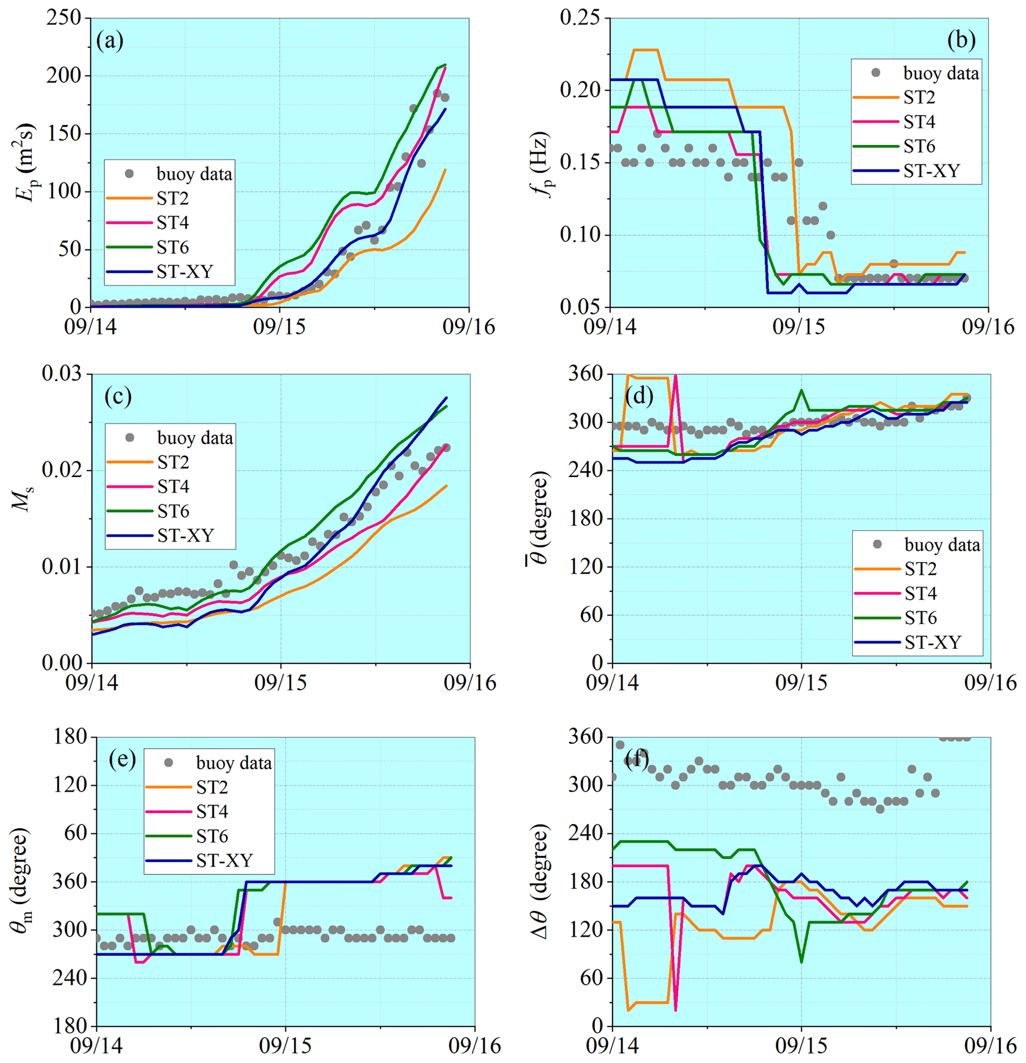
Figure 13 Comparisons of wave spectral parameters with observations at buoy 42039 during Hurricane Ivan: (a) spectrum peak value, (b) peak frequency, (c) mean square slope, (d) mean wave propagation direction, (e) main wave propagation direction and (f) wave propagation spread width.

4.2 Model setup

The computational domain, as shown in Fig. 10, covers the area affected by both Hurricane Ivan (2004) and Hurricane Katrina (2005), ranging from 100 to 82^∘ W and from 18 to 32^∘ N within the Gulf of Mexico. Considering a minimal time period for model warm-up, the simulation of Hurricane Ivan is initialized at 00:00 UTC on 12 September 2004 and continues for nearly 4 d until 21:00 UTC on 15 September 2004. The simulation of Hurricane Katrina is initialized at 00:00 UTC on 25 August 2005 and continues for nearly 7 d until 18:00 UTC on 31 August 2005. A time step of 10 min is fixed. The simulation is performed over the geographical coordinate system with a resolution of $\mathrm{1}/\mathrm{12}{}^{\circ }$. We assume 36 directional intervals with a constant increment of 10^∘ and 35 frequency intervals that increase logarithmically over the range of 0.0373–1.048 Hz. The numerical results obtained with the ST-XY source-term option are compared to those obtained with other options. The ST2, ST4 and ST6 options are implemented with the default setting.

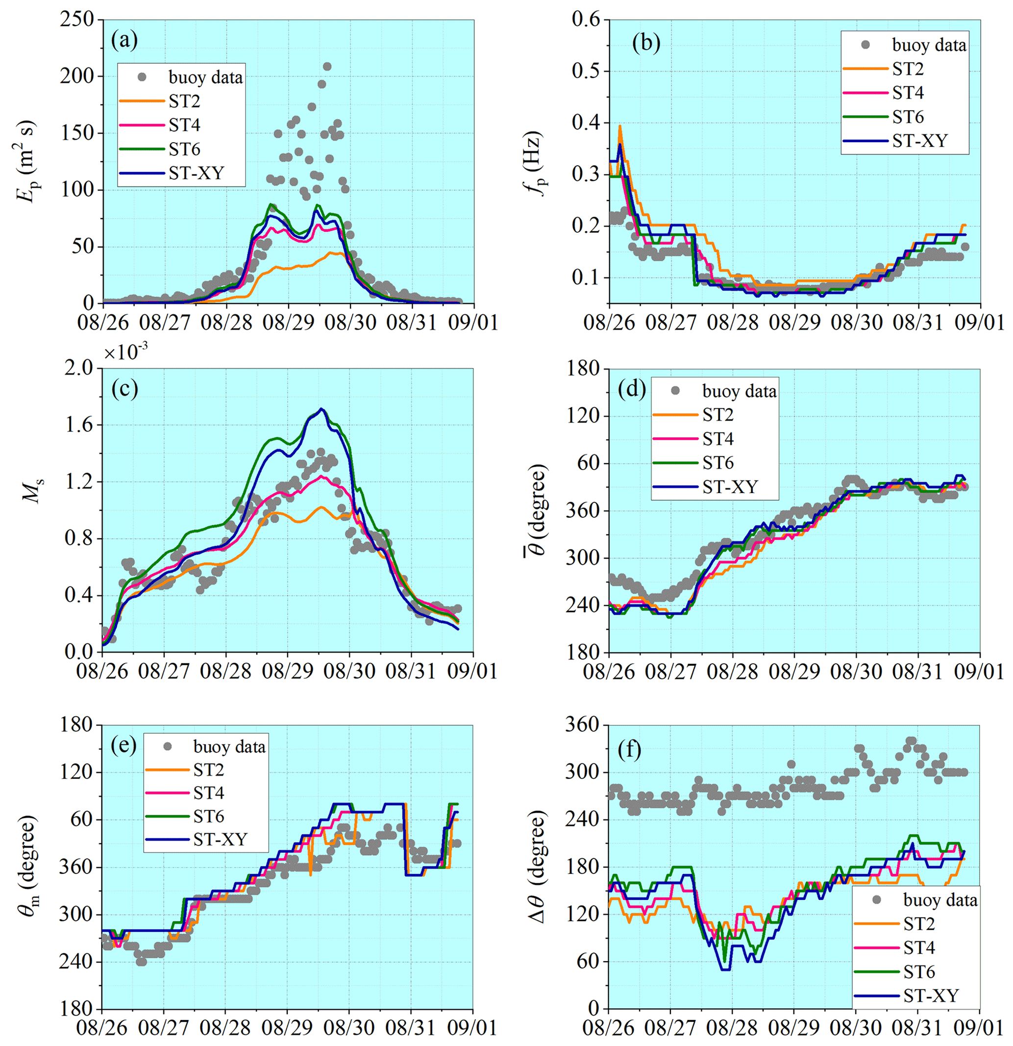
Figure 14 Comparisons of wave spectral parameters with observations at buoy 42039 during Hurricane Katrina: (a) spectrum peak value, (b) peak frequency, (c) mean square slope, (d) mean wave propagation direction, (e) main wave propagation direction and (f) wave propagation spread width.

4.3 Comparison of wave parameters

The model results on the time variations in the significant wave height H_s and the mean wave period T₀₂ at the locations of the buoys during Hurricane Ivan and Hurricane Katrina are shown in Figs. 11 and 12, respectively. The observed data are also plotted for comparison. It can be seen that the significant wave height H_s obtained with the ST-XY option agrees fairly well with the buoy data and performs better than the ST2 and ST6 options. The peak value and peak time of the significant wave height are accurately represented. In comparison, the significant wave height H_s is obviously overestimated by the ST6 option but underestimated by the ST2 option. The ST4 option also performs very well but still shows some underestimation of the peak values of H_s (as shown in Figs. 11a and 12a) and some overestimation of H_s before it reaches its maximum value (as shown in Fig. 11b–d). The numerical results for the mean wave period T₀₂ are shown to be generally less accurate than those for the significant wave height H_s, especially during the period before and after the hurricane event. A possible reason is that the total wave energy is paid more attention when formulating source terms of the wave model, while the statistical laws for wave period are usually less accurate under relatively calm-sea conditions. Note that an underestimation of T₀₂ is evident, but the peak values of T₀₂ are still reasonably simulated. The mean absolute error (MAE) and root mean square error (RMSE) for each hurricane event are shown in Tables 1 and 2. It is demonstrated that the ST-XY has outstanding performance on H_s with obviously smaller MAE and RMSE values. The performance of ST4 is also satisfactory as compared to ST2 and ST6.

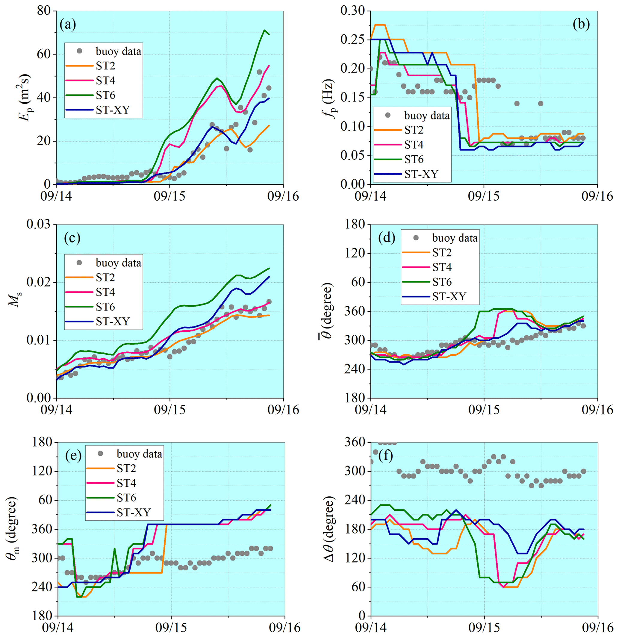
Figure 15 Comparisons of wave spectral parameters with observations at buoy 42036 during Hurricane Ivan: (a) spectrum peak value, (b) peak frequency, (c) mean square slope, (d) mean wave propagation direction, (e) main wave propagation direction and (f) wave propagation spread width.

4.4 Comparison of wave spectra

For the detailed description of a wave spectrum, the peak value E_p and the peak frequency f_p of the spectrum as well as its mean square slope M_s are defined to describe the frequency spectrum; the dominant wave propagation direction θ_m, the mean wave propagation direction $\stackrel{\mathrm{‾}}{\mathit{\theta }}$ and the directional spreading width Δθ are defined to describe the directional spectrum. In particular,

$$\begin{array}{}\text{(14)}& {\displaystyle }{E}_{\mathrm{p}}=max\left(\underset{\mathrm{0}}{\overset{\mathrm{2}\mathit{\pi }}{\int }}E\left(f,\mathit{\theta }\right)\mathrm{d}\mathit{\theta }\right),\text{(15)}& {\displaystyle }{M}_{\mathrm{s}}=\int \int k^{\mathrm{2}}E\left(f,\mathit{\theta }\right)\mathrm{d}f\mathrm{d}\mathit{\theta },\text{(16)}& {\displaystyle }E\left({\mathit{\theta }}_{\mathrm{m}}\right)=max\left(\int E\left(f,\mathit{\theta }\right)\mathrm{d}f\right),\text{(17)}& {\displaystyle }E\left({\mathit{\theta }}_{\mathrm{e}}\right)\ge \mathrm{0.1}max\left(\int E\left(f,\mathit{\theta }\right)\mathrm{d}f\right),\text{(18)}& {\displaystyle }\stackrel{\mathrm{‾}}{\mathit{\theta }}={\displaystyle \frac{\mathrm{1}}{\mathrm{2}}}\left({\mathit{\theta }}_{\mathrm{e}\mathrm{1}}+{\mathit{\theta }}_{\mathrm{e}\mathrm{2}}\right),\text{(19)}& {\displaystyle }\mathrm{\Delta }\mathit{\theta }={\mathit{\theta }}_{\mathrm{e}\mathrm{2}}-{\mathit{\theta }}_{\mathrm{e}\mathrm{1}},\end{array}$$

where E_p is the peak value of the frequency spectrum and f_p is the corresponding peak frequency; M_s is the mean square slope of the frequency spectrum, representing the effect of high-frequency wave components; E(θ_m) is the peak of the directional spectrum; θ_m is the corresponding direction, called the main wave direction; θ_e is called the efficient wave direction beyond which the wave energy is below 10 % of the peak value of the directional spectrum; θ_e1 and θ_e2 are the lower and higher limits of θ_e; and $\stackrel{\mathrm{‾}}{\mathit{\theta }}$ is the mean wave propagation direction, while Δθ is the directional range of the effective wave propagation.

Comparison of the computed wave spectra with observations is made at the locations of buoys 42039 and 42036, where a relatively complete data series has been recorded during both hurricane events. Variations in the spectral wave parameters in the deep-water condition (at buoy 42039) are presented in Figs. 13 and 14, while those in the shallow-water condition (at buoy 42036) are presented in Figs. 15 and 16. Accuracy of the numerical results for the peak spectrum value E_p is quite similar to that for the representative wave parameters such as H_s. The result obtained with the ST-XY option can catch the extreme wave energy condition very well, while the ST6 option always overestimates and the ST2 option underestimates it. The result obtained with the ST4 option overestimates E_p under the moderate wind conditions before the extreme events. The numerical results for the peak frequency f_p agree with observations well during both hurricane events. M_s is also satisfactorily simulated, which means that the high-frequency part of the wave spectrum is well described by the numerical model. It may be necessary to point out that, different from the results for the representative wave parameters, the peak of E_p may not be correctly represented by any package of the source terms under our consideration in some cases, as shown in Fig. 14a.

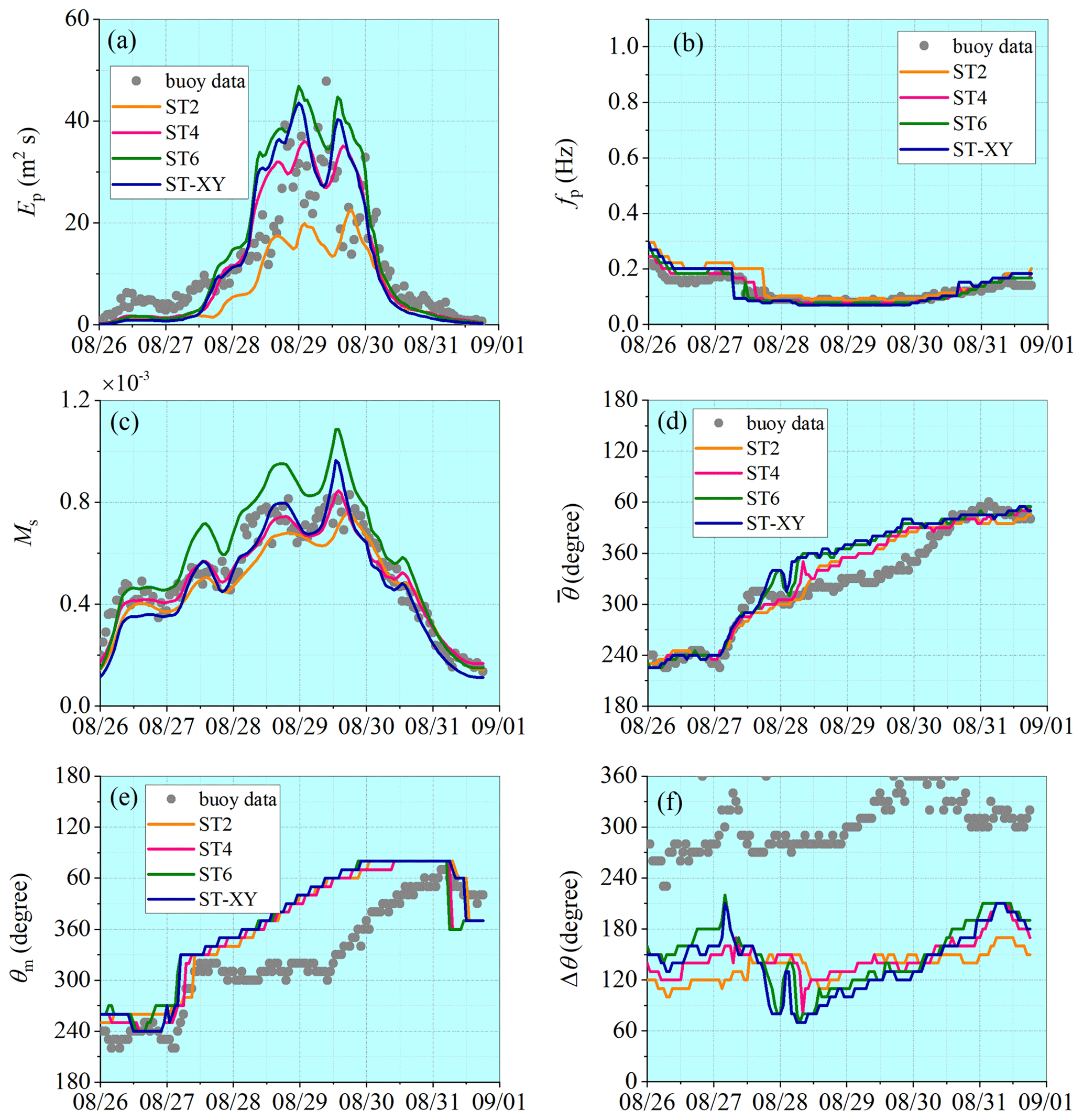
Figure 16 Comparisons of wave spectral parameters with observations at buoy 42036 during Hurricane Katrina: (a) spectrum peak value, (b) peak frequency, (c) mean square slope, (d) mean wave propagation direction, (e) main wave propagation direction and (f) wave propagation spread width.

It is also demonstrated that the numerical results for the main wave propagation direction and the mean wave propagation direction obtained with the ST-XY option and other source-term options are all equally good. However, the numerical result for the directional range of the effective wave propagation is obviously narrower than the observed one. This, however, may not be an error in the numerical model since the directional range of the effective wave propagation depends significantly on the methods employed (Earle et al., 1999; Kim et al., 1994). In this study, Longuet-Higgins' method (Longuet-Higgins et al., 1963) is used to build the directional wave spectrum from observed data. This method always leads to a broader directional spectrum than other methods with the same parameters (Fig. 2 of Earle et al., 1999).

Waves under hurricane conditions break more frequently and severely than under normal conditions due to high wind speed and rapidly transforming wind direction, leading to a relatively large amount of wind energy input into the breaking-wave components and also an increased total wind energy input. On the other hand, severe wave breaking under hurricane conditions also causes high wave energy dissipation. Therefore, a careful consideration of the effect of wave breaking is very important for the simulation of wave development under the action of tropical cyclones. Since evolution of the wave spectrum depends on the net effect of the wind energy input and the wave energy dissipation, while it is difficult to identify a decrease in wind energy input from an increase in wave energy dissipation, particularly under an extreme sea state, we emphasize that the wind energy input proposed by Xu and Yu (2020) and the wave energy dissipation extended from that of Ardhuin et al. (2010) must be considered a set.

5 Conclusions

This study aimed to evaluate the performance of the improved formulas for the wind energy input and the wave energy dissipation, i.e., the ST-XY source-term option. The numerical results are obtained with the coupled AWBLM–WWIII model. Both duration-limited waves under idealized conditions and hurricane-generated waves in both deep and shallow waters are studied. The standard source-term packages of ST2, ST4 and ST6 embedded in WWIII are chosen for comparison. Detailed comparisons are made for not only the representative wave parameters, including the significant wave height, the mean wavelength and the mean wave period, but also the characteristic parameters for the frequency spectrum and the directional spreading function. The effect of breaking on ocean wave modeling is fully discussed.

The numerical results show that the ST-XY source-term package performs better than other standard options in general. At the early wave-development stage, the ST-XY option leads to a better agreement of the computed wave energy with the empirical results, while other source-term options all tend to underestimate the wave energy. At the equilibrium stage, the results obtained with the ST-XY option approaches the Pierson–Moskowitz limit, while the ST2 option significantly underestimates the wave energy. The ST-XY option is also effective for ocean wave modeling under both deep- and shallow-water conditions and gives results in good agreement with field data. For hurricane-generated waves, model results obtained with the ST-XY option agrees well with the buoy data and are obviously better than those obtained with other source-term options. On the other hand, the ST6 option often overestimates wave energy, while the ST2 option leads to an obvious underestimation. The ST4 option performs fairly well but still shows some underestimation of the peak value of significant wave height and some overestimation of the significant wave height before its peak value is achieved.

Wave breaking significantly affects ocean wave modeling, especially at younger wave ages and in shallower waters. At the early wave-development stage, a significant part of the peak wind energy input takes place under breaking conditions, and the proportion decreases gradually as the wave development continues. In shallow waters, the peak value of wind energy input taking place under breaking conditions is always higher than that under non-breaking conditions throughout the early wave-development stage to the equilibrium stage.

In summary, the improved formula of Xu and Yu (2020), which includes both the breaking effect and the effect of airflow separation on the leesides of steep wave crests in a consistent way, has a satisfactory performance within the coupled AWBLM–WWIII model. It is physics-based and is verified to be effective for ocean wave modeling under both moderate and extreme wind conditions, at all wave-development stages, and in deep to shallow waters, thus having a broad applicability.