the Creative Commons Attribution 4.0 License.
the Creative Commons Attribution 4.0 License.
 | 24 May 2023
A generalized spatial autoregressive neural network method for three-dimensional spatial interpolation
Junda Zhan
Sensen Wu
Jin Qi
Jindi Zeng
Mengjiao Qin
Yuanyuan Wang
Zhenhong Du
Spatial interpolation, a fundamental spatial analysis method, predicts unsampled spatial data from the values of sampled points. Generally, the core of spatial interpolation is fitting spatial weights via spatial correlation. Traditional methods express spatial distances in a conventional Euclidean way and conduct relatively simple spatial weight calculation processes, limiting their ability to fit complex spatial nonlinear characteristics in multidimensional space. To tackle these problems, we developed a generalized spatial distance neural network (GSDNN) unit to generally and adaptively express spatial distances in complex feature space. By combining the spatial autoregressive neural network (SARNN) with the GSDNN unit, we constructed a generalized spatial autoregressive neural network (GSARNN) to perform spatial interpolation in three-dimensional space. The GSARNN model was examined and compared with traditional methods using two three-dimensional cases: a simulated case and a real Argo case. The experiment results demonstrated that exploiting the feature extraction ability of neural networks, the GSARNN achieved superior interpolation performance and was more adaptable than inverse distance weighted, ordinary Kriging, and SARNN methods.
- Article
(9422 KB) - Full-text XML
- BibTeX
- EndNote


Due to the difficulties of establishing abundant observation stations and the existence of unobservable positions in space, research areas in geospatial subjects typically contain many unsampled data points. Estimating unknown data based on sampled point values and expanding discrete and sparse data into continuous field are the main goals of spatial interpolation models. Spatial interpolation is widely applied in many research fields, including air quality (Tang et al., 2017), climate and hydrology (Arowolo et al., 2017; Adhikary et al., 2017; Cheng et al., 2017), marine environment (Gao et al., 2020; Zhang et al., 2021), ecosystem (Pan et al., 2021), city (Hu et al., 2013; Szczepańska et al., 2020; Ma et al., 2019; Aumond et al., 2018), and agriculture (da Silva Júnior et al., 2019). Therefore, accurately fitting the spatial correlation between elements and improving model spatial interpolation abilities are important for exploring spatial distribution patterns and change trends and solving myriad problems encountered in nature and society.
According to Tobler's first law of geography, “everything is related to everything else, but near things are more related to each other” (Tobler, 1970). It proposes the existence of spatial correlation, which is a general feature of geospatial data as well as a core theory supporting spatial interpolation modeling. Following spatial correlation theory, most spatial interpolation methods define the value of an unknown point as the weighted sum of the values of surrounding sample points. In the spatial weight calculation process, spatial distance is the most fundamental and direct data used to measure spatial correlation. Therefore, (i) the expression of spatial distance and (ii) the solution method and precision of spatial correlation weights are the key to spatial interpolation modeling and determine the reliability of interpolation prediction. In fact, interpolation can be regarded as the problem of mining complicated nonlinear relationships between spatial distances and spatial weights.
Since the 1950s, scholars have proposed various classical spatial interpolation methods through extensive practical explorations, including inverse distance weighted (IDW), Kriging, natural neighbor, spline, trend surface, and radial basis function, and they can use sampled points to model and restore spatial feature fields to a certain extent. Many studies have been conducted to improve and reform the traditional methods from the following perspectives: design search strategy of adjacent sampled points (Babak and Deutsch, 2009; Sun et al., 2020), change the measuring method of spatial distance (Greenberg et al., 2011; Aumond et al., 2018), change the calculation method of spatial weights based on data distribution characteristics (Lu and Wong, 2008; Li et al., 2020), incorporate other variables and information (Kumar et al., 2012; Adhikary et al., 2017), and improve the efficiency of interpolation calculation (Liang et al., 2018; Wang, 2015). However, most methods are still based on simple mathematical formulas and parameter calculations and have difficulty describing nonlinear and complex relationships in spatial processes. These limitations prevent these interpolation approaches from accurately reflecting the relevant characteristics of geographical elements, restricting their spatial interpolation abilities.
In recent years, machine learning theories have developed rapidly, which has provided new solutions for accurate spatial interpolation. A number of strategies and models of machine learning were introduced to solve interpolation problem, such as random forest (da Silva Júnior et al., 2019; Sekulić et al., 2020), support vector machine (Li et al., 2018; X. Zhang et al., 2017), and neural network (Rigol et al., 2001; Kanevski et al., 2008; Tao et al., 2019; Zeng et al., 2020). These models enable spatial interpolation methods to fit the nonlinear features. In particular, Zeng et al. (2020) proposed the spatial autoregressive neural network (SARNN) model for two-dimensional spatial interpolation by integrating the neural network with spatial autoregression theory, achieving superior performance compared with traditional spatial interpolation methods. However, these methods still lack consideration for the sufficient expression of spatial distance and their applicability in three-dimensional spaces with more complex feature fields.
With regard to spatial distance expression, traditional methods and the SARNN model employ Euclidean distances calculated using a fixed formula, treating all directions in space equivalently. However, spatial anisotropy, the universal feature of spatial element distribution and change, should be considered for accurate spatial interpolation, especially in three-dimensional space (Wu et al., 2020). For example, mineral resource distribution exhibits directional differences affected by geological structures (Samal et al., 2011), soil nutrient content gradients have specific orientation patterns (Abd El-Hady et al., 2018), and climate elements such as surface temperature and precipitation can be strongly direction-dependent on spatial scales (Chen et al., 2016; Y. Zhang et al., 2017; Wang et al., 2018). In three-dimensional spatial interpolation, spatial isotropic distance expression implies that any point with the same distance from a target point will exert the same effect on it, even if they are from different directions. It ignores the effects of differences and the complex coupling of various spatial axes on spatial weights, resulting in insufficient spatial correlation mining.
To address these limitations, we propose a generalized spatial distance neural network (GSDNN) unit to express distances in multidimensional space with nonlinear characteristics. In the GSDNN, generalized spatial distances between elements are fitted using multidirectional distance components. Furthermore, by combining the GSDNN unit with the SARNN, we integrated generalized distances into the spatial interpolation method and developed a generalized spatial autoregressive neural network (GSARNN) model to realize complex nonlinear spatial interpolation modeling in three-dimensional space, improving spatial interpolation prediction and fitting abilities.
The remaining sections of this paper are organized as follows. Section 2 briefly introduces two traditional interpolation methods; defines the SARNN model and GSDNN unit; and describes the overall GSARNN model framework, training strategy, and evaluation method. In Sect. 3, we perform interpolation experiments on two cases and compare the IDW, Kriging, SARNN, and GSARNN model results. The discussion and conclusion are given in Sects. 4 and 5, respectively.
2.1 Traditional spatial interpolation
Interpolation methods can be divided into deterministic interpolation and geostatistical interpolation approaches, according to their mathematical principles. Deterministic interpolation, such as IDW, spline, and trend surface methods, builds the fitting surface according to the smoothness of the whole spatial surface or the similarities of spatial information elements to predict data in unknown regions. Geostatistical interpolation, such as the Kriging method, builds the sample point spatial structure by analyzing the distribution laws and relevant features of the sample points in space and predicting the change trend of the whole spatial area.
2.1.1 IDW interpolation
IDW interpolation (Shepard, 1968) is a deterministic interpolation method (Watson and Philip, 1985). IDW regards the value at an unsampled location as the distance-weighted average of the sampled point values (Longley et al., 2011). For an unsampled point, the closer the sampled point is, the greater an influence it exerts; the influence is inversely proportional to the distance. IDW can be expressed as
where is the predicted value at the unsampled point i, zj is the observed value of point j, dij is the Euclidean distance between point i and point j, and p is the power parameter that defines the weight decline rate as the distance increases. By defining a larger p, the influence of closer points is strengthened, affecting the smoothness of the interpolation results.
Due to the simplicity, convenience, and intuitiveness of the IDW method, it has been widely used in many fields, including geography, agriculture, oceanography, and environmental studies; however, extreme values among the sampled points can have a substantial impact on IDW spatial prediction results.
2.1.2 Kriging interpolation
Kriging methods, such as ordinary Kriging (OK), universal Kriging, and co-Kriging, are spatial interpolation methods designed to solve the problems of mineral deposit predication and error estimation (Krige, 1952; Matheron, 1963). These methods generate unbiased optimal variable estimations in a finite area using the variation function to perform moving average interpolation according to the differences of the sample points' positions and spatial correlation degree. Among the Kriging methods, OK is the most commonly used.
Kriging can be expressed as
where z∗(x0) is the predicted value, and λi and z(xi) are, respectively, the weight coefficient and observed value of point i.
Kriging methods involve the calculation of the weight coefficient λi, for which the key is to satisfy the unbiasedness and optimality. Unbiasedness means that z∗(x0) is the unbiased estimate of z(x), that is
which can derive the following constraints on λi:
Optimality means that z∗(x0) is the optimal estimate of z(xi), and the variance between the predicted value of the unsampled points and the estimated value of the observed points is the smallest, that is
Define the cost function and try to figure out a set of weights λi that satisfy unbiasedness and minimize the cost function. Finally, the following equation set can be derived:
where rij is the semi-variogram between point i and point j, which can be expressed as
where σ2 is the variance of z(x), which is a constant in OK. rij can be simply determined by zi and zj. Kriging assumes that there is a functional relationship between rij and dij (the distance between point i and point j). By taking any two sampled points from the dataset, a total of pairs can be generated. We can use a linear, Gaussian, spherical, or exponential model to fit the relationship between rij and dij. Using the fitted function, we can calculate rj0 through dj0. Thereby, the optimal weight set λi for Eq. (2) can be solved through Eq. (6).
2.2 SARNN model
Summarizing the principles of most traditional interpolation methods, it can be found that they are modeled following the core concept of fitting the relationship between spatial distance and spatial weight, a relationship that is often complicated, containing nonlinear characteristics. Thus, achieving accurate fitting using only simple mathematical functions is difficult. Establishing a nonlinear expression between the spatial distance dij and the weight coefficient wij is necessary to interpolate unsampled points from observed points. The spatial weight of sampled points to point i is defined as
where wi represents the spatial weight vector of point i, wij is the spatial weight of point j to point i, and is the spatial distance between point i and point j.
To characterize complex nonlinear relationships in space, Zeng et al. (2020) designed the SARNN model, exploiting the powerful modeling and nonlinear fitting capabilities of neural networks to fit the spatial weight wi.
It should be noted that there is a weight wii in the vector wi which represents the spatial weight of point i to itself. To avoid overfitting, this weight should be set to 0:
The spatial weights of all sampled point pairs can be expressed by an n⋅n weight matrix W. According to Eq. (9), the weights on the diagonal of W should be reset to 0. Therefore, W can be defined as
where ρ is the spatial weight component, and K is the standard weight component, which ensures that the neural network weight is independent of the point itself in the training process. kij in K can be expressed as
Next, the problem of solving the spatial weight can be transformed into the problem of constructing and training the neural network. The distance from the point to be interpolated to the observed point is the network input, the hidden layers are defined, and the spatial weight vector ρi is the output, that is
where represents the vector of distances from point i to other sample points, and ρij represents the spatial weight of point j to point i. ρij is correspondingly multiplied by kij to obtain the weight coefficient wij. The matrix form is as follows:
The product of the final spatial weight matrix W and the sampled value vector y is the unsampled point estimation results. can be expressed as
2.3 GSARNN model
2.3.1 Model definition
Spatial distance is the most important indicator of the relationship between two objects as well as the basis of spatial weight fitting. The essence of spatial interpolation is establishing a distance-based mapping relationship between the sampled region and the unsampled region.
For any two vectors α, β in the n-dimensional linear space V, there are a pair of coordinates and under the orthonormal basis. There are many ways to define spatial distances, such as the Manhattan distance, Euclidean distance, and Minkowski distance, which can be expressed as
The traditional two-dimensional spatial interpolation methods always use Euclidean spatial distance as the basis for expressing spatial correlation, treating different spatial relative positions equivalently. However, in geographic space – especially in three-dimensional and higher-dimensional spaces – the changing trend and rate of elements often differ along various axes, and there is local variability in the data. Using Euclidean distance for three-dimensional spatial interpolation is an isotropic solution (Allard et al., 2016) that reduces the dimensionality of the raw data, discards a large amount of relative position information between points, and cannot adequately reflect the complicated nonlinear characteristics of data change, restricting the accuracy of interpolation in multidimensional linear space.
To solve these problems, we propose a generalized expression of spatial distance. The generalized spatial distance of α and β in n-dimensional linear space is defined as the function of the coordinate difference under the orthonormal basis, which can be expressed as
The distance components of the point to be interpolated and the known sample point under the three-dimensional orthonormal basis are
To fully and adaptively capture the nonlinear effect of the elements' changing trend in three-dimensional space, we designed a GSDNN unit that generates generalized spatial distances considering anisotropy based on the distance components of each axis. It can be simply expressed as
Through network training, the generalized spatial distance automatically output by this network unit will reflect the complex characteristics of the specific spatial elements. The GSDNN structure is shown in the dashed box in Fig. 1.
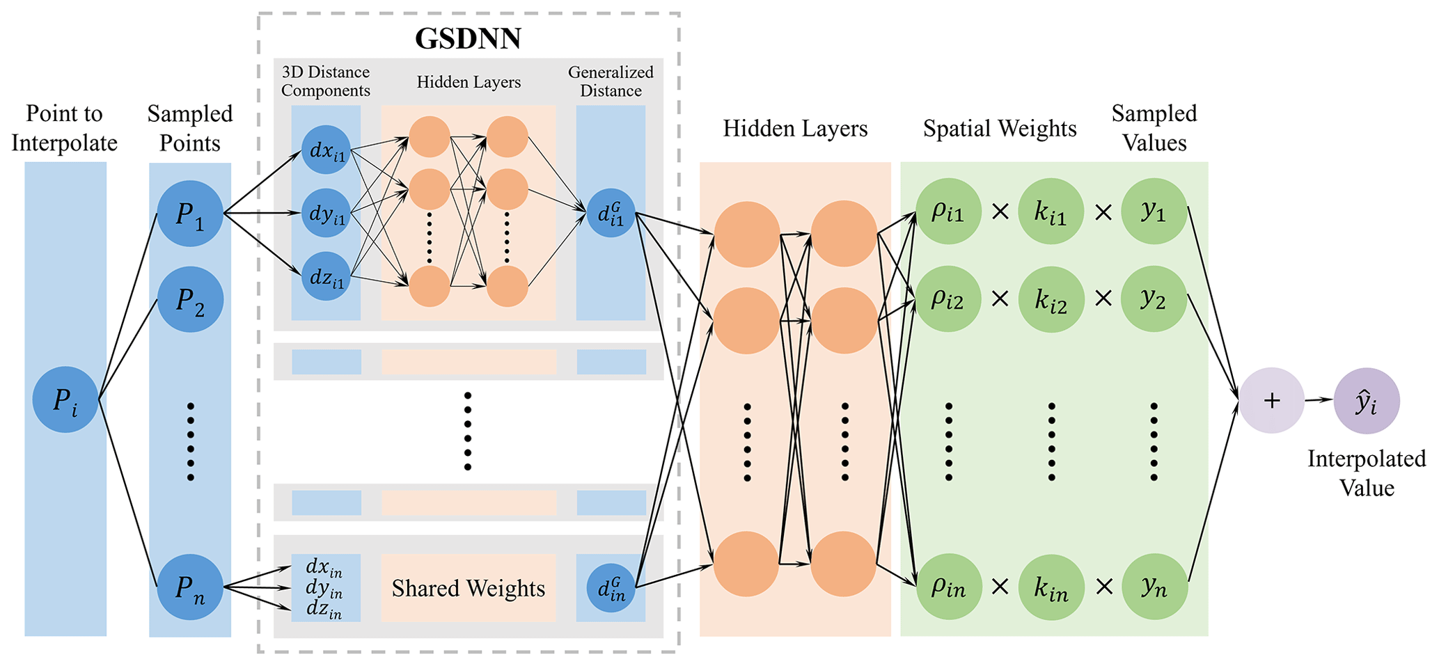
By replacing the input of the SARNN model with the GSDNN unit, Eq. (12) can be refined as
The refined model is the GSARNN model, and the overall model structure is shown in Fig. 1.
In the modeling process, the distance components from the unknown point to the sampled points in three-dimensional space are input into the GSDNN, and all GSDNN units share network weights and biases. Through the training process, the generalized spatial distance between the two points under the specific spatial context of the interpolation element is output and simultaneously becomes the input of GSARNN. After the hidden layer calculations, the output layer finally outputs the spatial weight component, which is multiplied by the standard weight component and the observed values of the sampled points. The sum of the output tensor is the interpolated value of the unsampled point. Note that since there is no recognized true value of generalized spatial distance for training process, the GSDNN unit can only be embedded in the neural-network-based method and participates in its overall training and calculation process. In other words, the generalized spatial distance is determined by the spatial characteristics of the elements to be interpolated, owning a specific connotation based on specific context of spatial elements.
2.3.2 Model design and estimation
To improve the transferability and adaptability of the GSARNN and solve the problems of overfitting and gradient vanishing in neural network training, we design a set of model training strategy based on the cross-validation method, including the overall training framework, parameter initialization method, activation function definition, and training optimization algorithms. A complete set of training processes is established to improve training quality and interpolation accuracy, as shown in Fig. 2.
We employ several neural network structure design and model optimization techniques to improve training efficiency. For each hidden layer, we first use the robust parameter initialization method proposed by He et al. (2015). Second, the batch normalization method of Ioffe and Szegedy (2015) is adopted to accelerate the model training convergence speed and improve the training process stability. Third, the PReLU (parametric rectified linear unit) proposed by He et al. (2015) is used as the activation function to improve model performance. Finally, the dropout strategy developed by Srivastava et al. (2014) is integrated to strengthen the generalizability of the model.
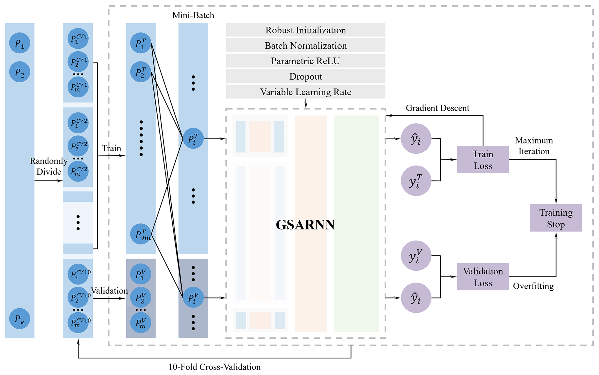
2.3.3 Model training and validation
We use the 10-fold cross-validation method for model training. The dataset is randomly divided into 10 equal portions, among which 9 portions serve as the training set, and the remaining portion is used as the validation set in turn. The training set is used to fit the data characteristics, and the validation set is used to verify the generalization performance of the model. The cross-validation method averages the training results of each group, reduces the sensitivity to data division, avoids overfitting to a certain extent, and extracts more effective features from the data.
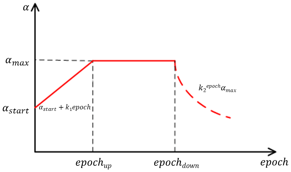
Learning rate selection is critical in network training. An excessive learning rate will lead to an oscillation of the loss and unavailability of the optimal solution. Conversely, an insufficient learning rate will result in slow convergence or even gradient vanishing. In view of the characteristics of the GSARNN model, we adopt a custom variable learning rate in the training process. The formula is as follows:
where αstart is the initial learning rate, which increases gradually at the rate of k1 until αmax. A relatively small initial learning rate can prevent an excessive fluctuation and convergence obstacle, and the following increment of the leaning rate can avoid the convergence rate at the early stage of the training process being too low. The maximum learning rate is maintained for n epochs. At this stage, the model can stably learn the spatial characteristics of the elements. The learning rate then gradually decreases exponentially at the rate of k2, ensuring that the model can sufficiently converge near the optimal position. The change of the learning rate throughout the training process is shown in Fig. 3.
The GSARNN model takes the mean square error (MSE) as the loss function in the training process:
2.4 Evaluation method
To quantitatively measure the performance of the IDW, OK, SARNN model, and GSARNN model methods, we use the determination coefficient (R2), root mean square error (RMSE), mean absolute error (MAE), and mean absolute percentage error (MAPE) as evaluation indicators. The formulas are as follows:
R2 is a relative indicator that compares the model with the baseline using the average value as the interpolation result. The RMSE, MAE, and MAPE are absolute indicators that reflect the interpolation error; smaller values indicate higher model accuracy.
We use two three-dimensional datasets with distinct characteristics to test the interpolation performance of the GSARNN model in different scenarios, comparing it with the traditional IDW and OK methods and the SARNN model. In case one, we conduct experiments using a simulated dataset, which can be generated arbitrarily and controllably. By simulating a dataset with complex features and conducting a quantitative cross-validation interpolation experiment on it, we can fully test the feature extraction and fitting ability of the GSARNN model. In case two, we experiment on a measured Argo temperature dataset in the western Pacific area, which reflects the authentic natural characteristics. In this case, in addition to the cross-validation interpolation, we select several spatial sections for interpolation prediction. By qualitatively analyzing the section interpolation results, the GSARNN model's ability to restore spatial element field patterns in practical interpolation applications is examined.
3.1 Case one: simulated dataset
To examine the ability of the GSARNN model to handle data with complex characteristics in three-dimensional space, we combine trends of gradual change and sudden variation to simulate a dataset in the three-dimensional spatial field, repeating the simulation and interpolation for 100 times.
3.1.1 Dataset
Defining the three-dimensional area of a cube with the unit length, the side length of the cube is 6, and the distance between adjacent data points is defined as 0.5. Therefore, the three-dimensional spatial research area contains data points, and the spatial coordinates of each point are generated according to the following formulas:
The simulated value V is defined as
V1 is a three-dimensional spatial data item with a gradual change trend, calculated as follows:
where are the coordinates of the sample point i in the three-dimensional spatial field. V1 has a gradual gradient along the direction, as shown in Fig. 4a.
V2 is a three-dimensional spatial data item with local spatial variability, calculated as follows:
V2 has a spatial mutation at the two spherical surfaces 1.5 and 3 units away from the center of the three-dimensional space. The values of the entire dataset appear to diffuse from the center of the sphere to the surroundings, as shown in Fig. 4b. V2 possesses high local spatial variability, which imposes certain challenges to the interpolation work.
The term ε is a random item that brings some uncertainty to the simulated dataset and can be expressed as
The final three-dimensional spatial simulated dataset V is generated by adding V1, V2, and ε, as shown in Fig. 4c. The figure shows that the simulated data have both the gradient feature from V1 and the mutation feature from V2.

Figure 4An example of a simulated dataset. (a) Component V1 with a gradual change trend; (b) component V2 with a mutation; (c) the simulated dataset combining V1, V2, and ε.
This case compares the interpolation abilities of the GSARNN model and the other three models in three-dimensional space using the simulated dataset above.
3.1.2 Experiment implementation
According to the data division method, the simulated dataset is randomly divided into 10 equal parts for the cross-validation experiments. Each experiment has 1555 data points in the training set and 173 data points in the validation set. The validation set interpolation results of each fold are merged to obtain the complete interpolated dataset.
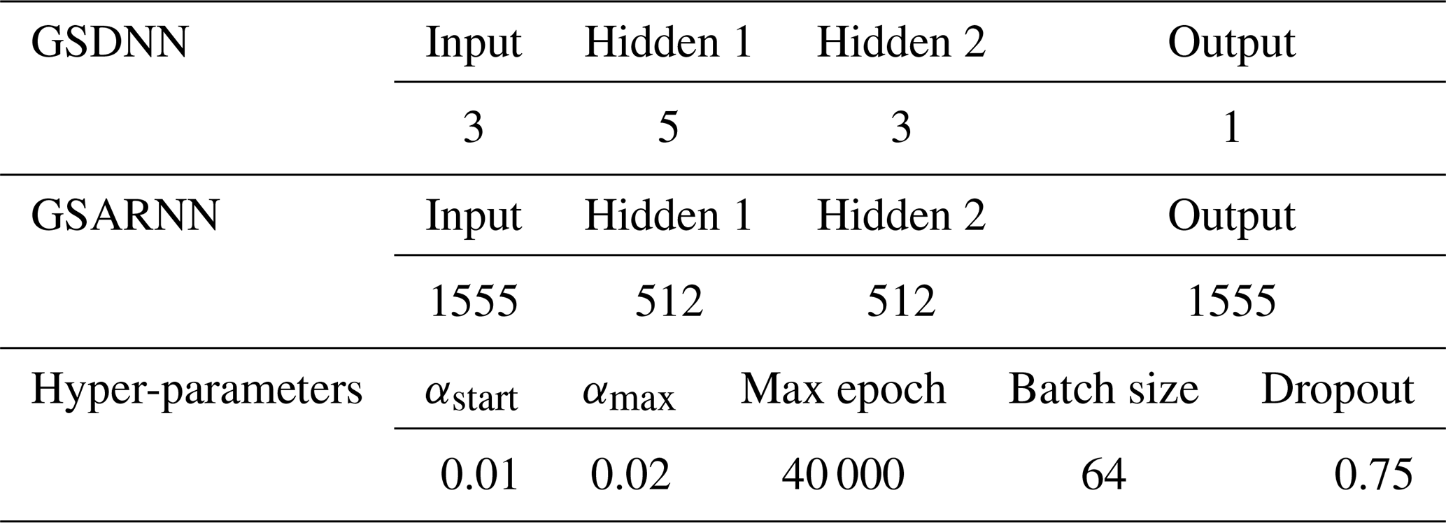
Considering that the four-layered feedforward network is a simple but efficient network structure (Tamura and Tateishi, 1997), we design the GSARNN architecture with one input layer, two hidden layers, and one output layer. The number of neurons in the input layer and output layer is equal to the number of sample points in the training set. There is no standard method to determine the optimal number of neurons in two hidden layers. Instead, we determine the optimal number using a simple combination strategy proposed by Du et al. (2020). Table 1 lists the optimal network structure settings and hyper-parameters of the GSARNN model in this case. Besides, the power parameter of the IDW method is 4, and in the Kriging method we adopt the Gaussian model to fit the functional relationship between the semi-variogram and the spatial distance, which turns out to be the optimal variation function model among linear, Gaussian, spherical, and exponential models. The generalized spatial distance output by the GSDNN unit serves as the input for the GSARNN model, while the three-dimensional spatial Euclidean distance serves as the input for the three comparison methods. The GSARNN and SARNN models are implemented using TensorFlow-GPU 1.13.0 and Python 3.5.4.
Table 1Network structure settings and hyper-parameters of the GSARNN model in case one.
3.1.3 Results
Under the same conditions, interpolation experiments are conducted on the three-dimensional simulated dataset 100 times using the IDW and OK methods and the SARNN and GSARNN models. The mean statistical indicator results of the cross-validation experiments are shown in Table 2. Compared with the traditional IDW and OK methods, the two neural network methods show significant improvements on all statistical indicators. The R2 value of the SARNN model (0.8804) is 19.62 % higher than that of the OK method (0.7360). After integrating the GSDNN unit, the R2 increases by 5.95 % to 0.9328 for the GSARNN, for an overall increase of 26.74 %. In addition, the RMSE, MAE, and MAPE values of the OK method are 1.4466, 1.0040, and 92.69 %, respectively, decreasing to 0.7298, 0.5280, and 40.99 %, respectively, for the GSARNN. Among the four models, the GSARNN model achieves the best performance in all indicators.
Table 2The mean statistical evaluation results of 100 experiments on the simulated dataset using the IDW, OK, SARNN, and GSARNN methods.
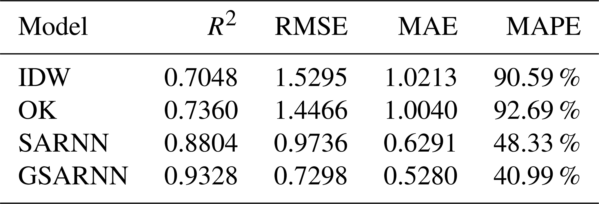
Figure 5 shows the three-dimensional diagrams of the simulated dataset example in Fig. 4 and its corresponding cross-validation interpolation results generated by the four methods. Taking the simulated dataset as a reference, all four methods express the overall change trend, but the IDW and OK methods perform poorly in the mutation area, which presents as the weakening of the mutation trend and the existence of an obvious interpolation transition zone. The interpolation results of the SARNN and GSARNN models capture and display the mutation characteristics well, and the overall pattern is basically consistent with the simulated data.
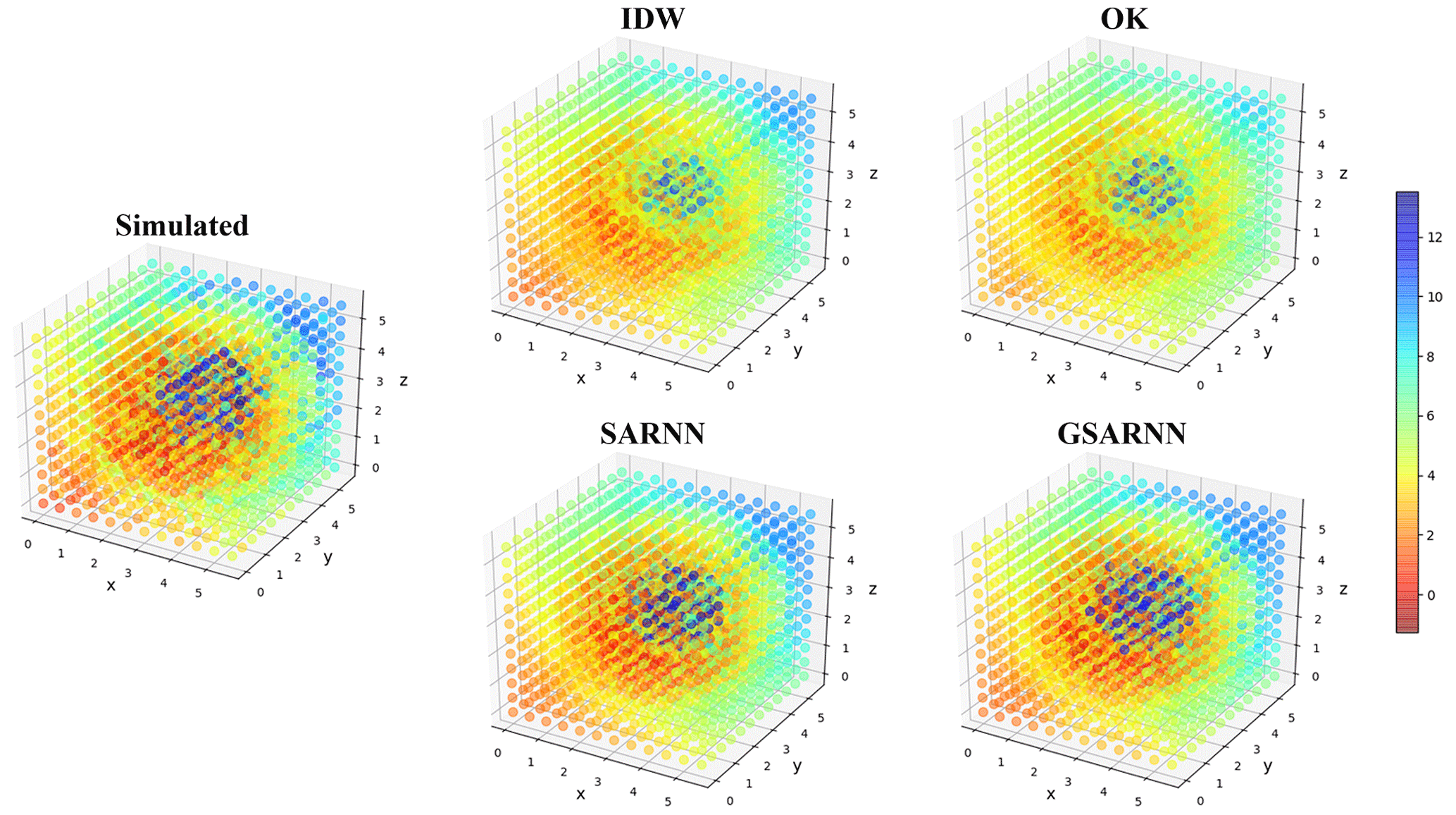
Figure 5Three-dimensional diagrams of the simulated dataset example in Fig. 4 and its corresponding cross-validation interpolation results.
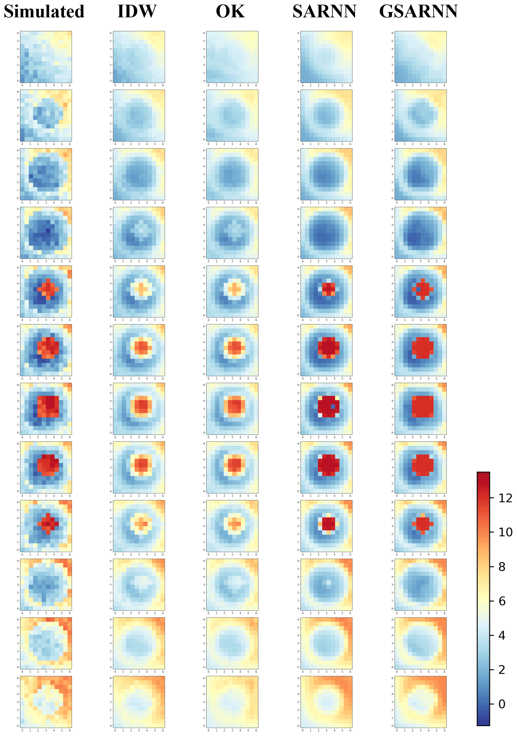
Figure 6 shows the detailed interpolation results of Fig. 5 in the form of section images, which are cut along the X–Y plane. In the IDW and OK method results, the low values of the mutation area are obviously overestimated, and the high values are underestimated. Moreover, under the influence of the central high value, unexpected imprints appear in the 4th and 10th layers, which reflects the limitations of traditional interpolation methods in handling mutation. The SARNN and GSARNN models largely restore the data characteristics of the simulated dataset, and the mutation is properly interpolated. Furthermore, the GSARNN model achieves more accurate results at the mutation interface.
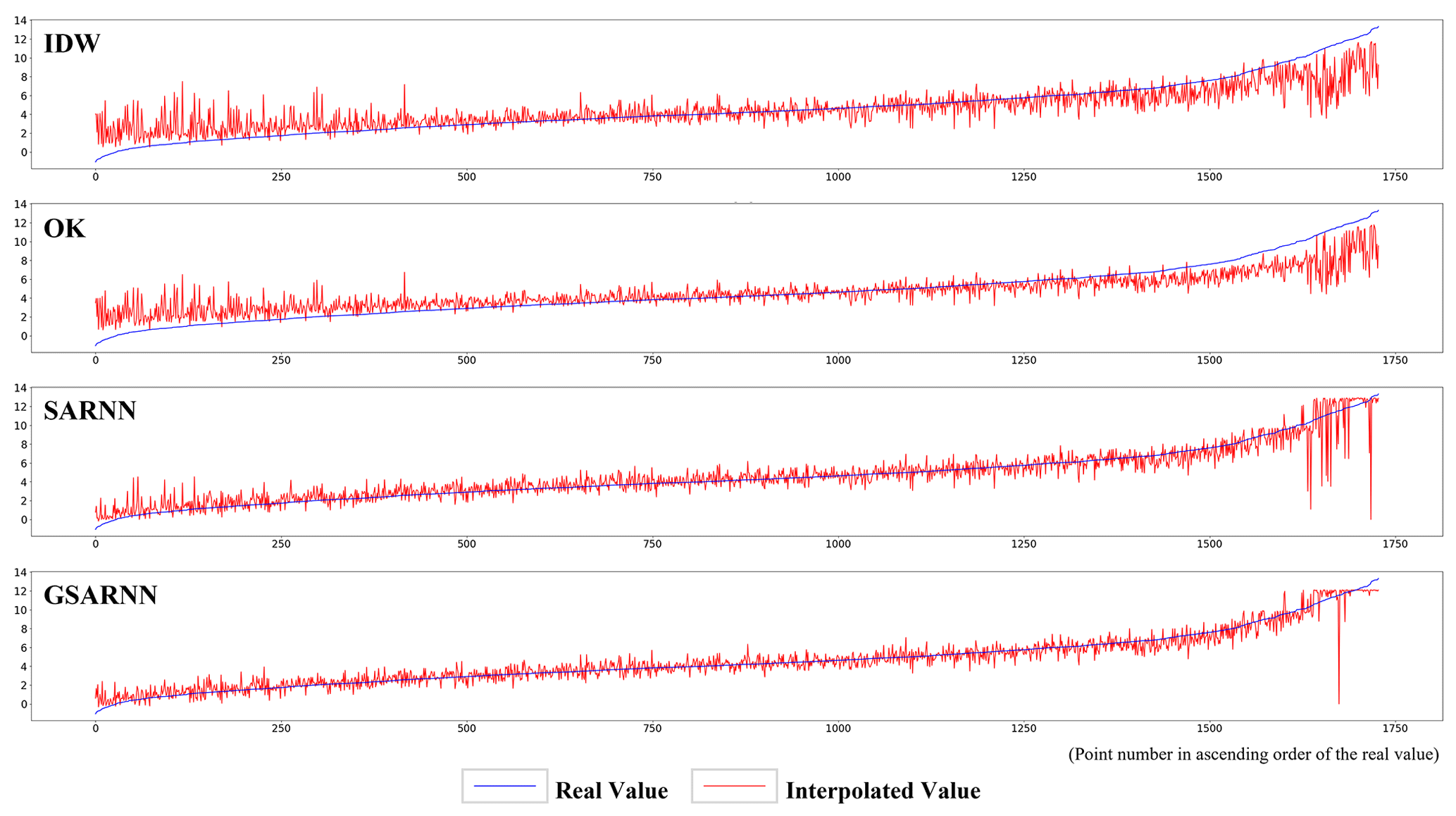
The real value and the cross-validation interpolation result values of the four models in Fig. 5 are drawn in line charts in Fig. 7. To evaluate the model performance in different value ranges, the line charts are drawn in ascending order of the real value, which is shown as a rising blue curve. The red line is connected by the model interpolation result points corresponding to the points in the simulated dataset, shown as a fluctuating broken line. In the median value area, the interpolation results of the four methods fluctuate relatively slightly near the real value. The IDW and OK method results show obvious low-value overestimation and high-value underestimation in a large range of low and high values, corresponding to both sides of the mutation interface. Limited by the interpolation mechanism and simplicity of traditional methods, it is difficult for them to interpolate elements containing mutation characteristics. However, the fluctuation amplitude and deviation degree of the OK method result are slightly smaller than those of the IDW method. The interpolation performance of the SARNN and GSARNN models in each value range is comparatively stable. Only a slight overestimation is observed in the low-value area, but there are individual points with large deviations in the high-value area. By contrast, the interpolating capacity of the GSARNN for mutant elements is significantly better than that of the SARNN.
In addition, compared with multifarious models in the fields of deep learning, the structure of GSARNN is relatively lightweight, so its training and calculation efficiency can be quite high. Taking advantage of mighty parallel computing capabilities of GPU units and distributed computing structures to accelerate the training process, the GSARNN model usually converges to the optimal state within 15–20 min in our cases. Although the efficiency of the Kriging method is better than the GSARNN model, under the same condition, it still takes about 10 min to fit the functional relationship between the semi-variogram and the distance.
3.2 Case two: Argo dataset
3.2.1 Study area and dataset
The second case uses the measured Argo ocean dataset. The study area is in the northern part of the western Pacific, which is located near the Equator, and is one of the main sources of atmospheric water vapor. The sea–atmosphere interaction in this area is strong and exerts certain influences on natural phenomena such as El Niño (Jian and Jin, 2008); therefore, it is of practical significance to conduct research in this region. Water temperature is one of the most important oceanographic elements. Because the western Pacific is the divergent center of three major monsoon circulations and multiple ocean currents converge here, the seawater temperature in this area has a substantial impact on the natural environment. This case uses the sea temperature in the western Pacific as the interpolation object.
Three-dimensional temperature data were obtained from the Argo (Array for Real-time Geostrophic Oceanography) project, which was initiated to study global oceanic climate change. The Argo observation network has launched 3000 profile buoys that measure the ocean temperature and salinity in the depth range of 2000 m (Riser et al., 2016). Argo data have become the main source of marine climate information and are widely used in marine and climate research (Liu et al., 2017). However, the Argo buoys are sparsely distributed, and the practical applications of the discrete data they collect are limited. Therefore, interpolating Argo data is necessary for generating a continuous data field and enhancing the practicability of the data products.
The data used in this case were obtained from China's Argo Real-time Data Center (http://www.argo.org.cn/, last access: 6 May 2022). The data collection time is early August 2018; the space range is 0–34∘ N, 115–160∘ E; and the depth range is 0 to 1000 m below the sea surface. The data include measurements from 144 buoy stations and 1944 monitoring items. The distribution of buoy stations on the sea surface is relatively uniform, as shown in Fig. 8.
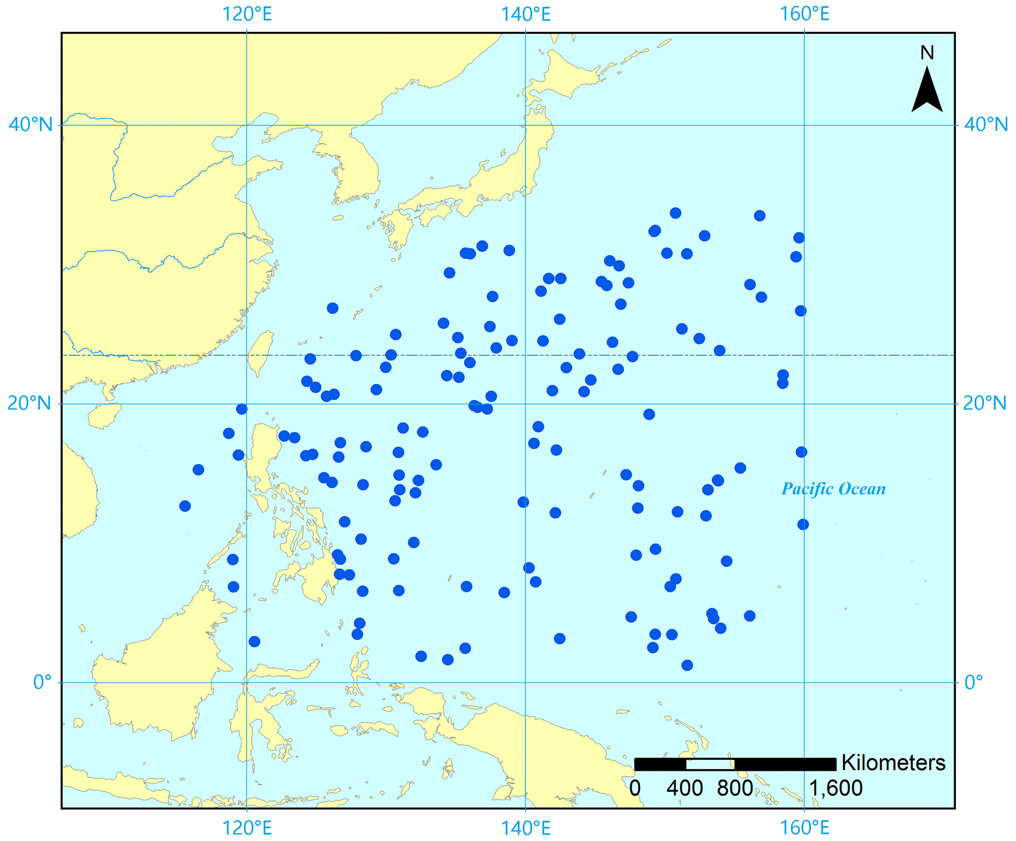
Figure 8Distribution map of Argo buoy stations represented by blue points, 144 stations in total (the base map is from ESRI maps).
A three-dimensional visualization of the Argo dataset is shown in Fig. 9. The temperature field data in the western Pacific region are distributed regularly, with obvious and uniform variation trends and strong spatial correlation. Little temperature variation is observed in the longitudinal direction. In the latitudinal direction, the boundary between the low-temperature region and the high-temperature region sinks obviously, and the overall temperature increases with increasing latitude from 0 to 35∘ N. In the vertical direction, the temperature decreases gradually with increasing water depth. The mean, minimum, maximum, and standard deviation of the Argo temperature dataset are shown in Table 3.
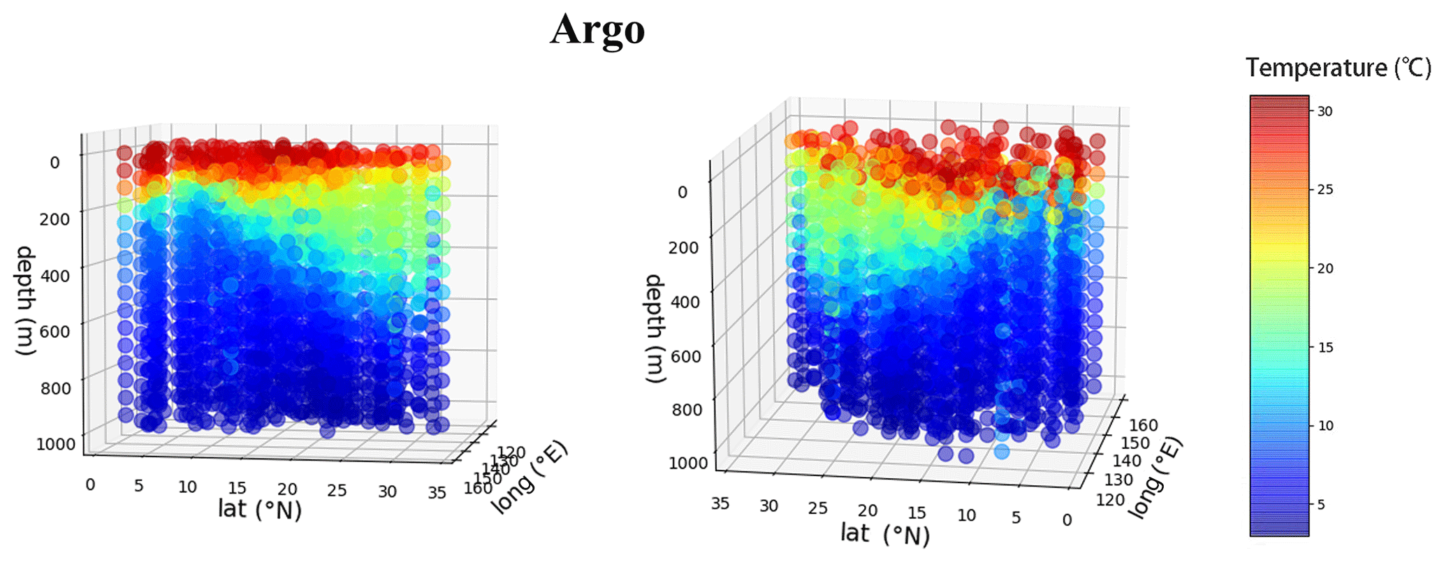
Table 3Basic statistics of the Argo temperature dataset with 1944 monitoring points in total.
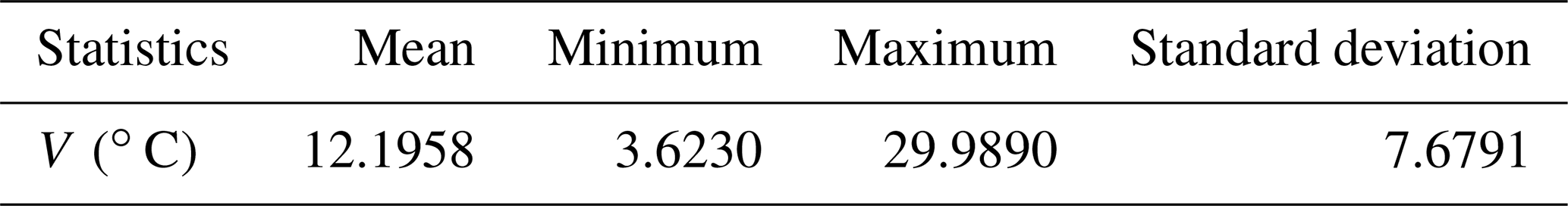
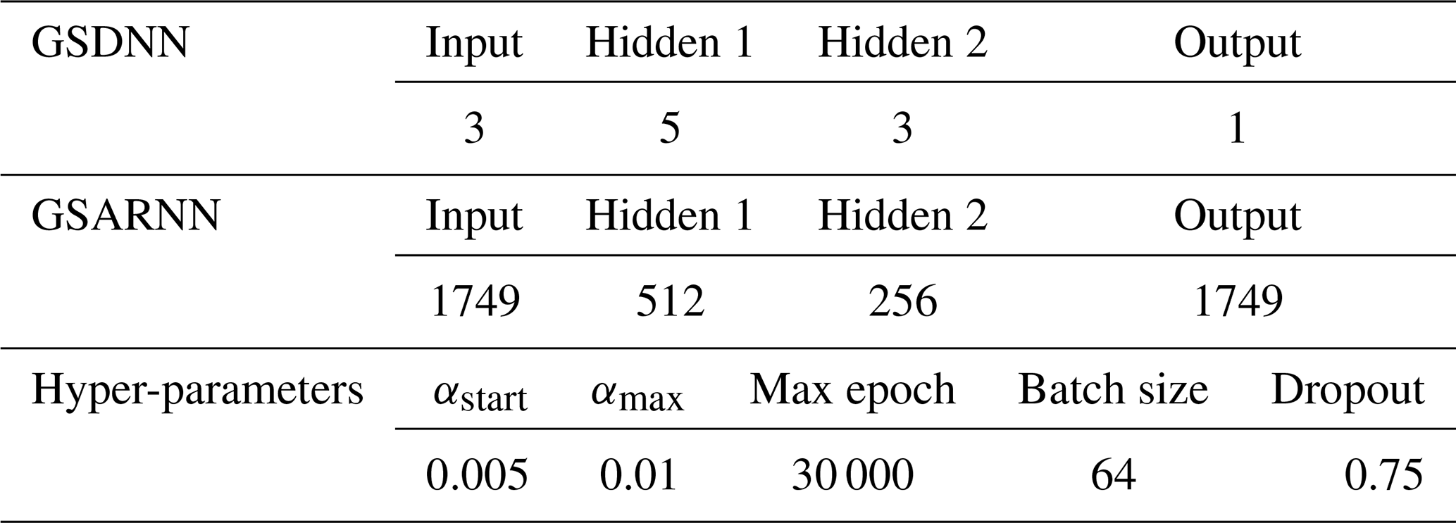
Table 4Network structure settings and hyper-parameters of the GSARNN model in case two.
This case compares the interpolation abilities of the GSARNN model and the other three models in three-dimensional space using real temperature data collected by Argo buoys.
3.2.2 Experiment implementation
The model details are determined in a similar way to case one. The optimum network structure settings and hyper-parameters of the GSARNN model for case two are listed in Table 4.
3.2.3 Results
Under the same conditions, interpolation experiments are conducted on the three-dimensional measured Argo dataset using the IDW, OK, SARNN model, and GSARNN model methods. The statistical indicators for the cross-validation experiments are shown in Table 5. In contrast to the simulated dataset of case one, the values of the Argo dataset mainly change in a gradual manner, which is relatively simple. Therefore, all four methods achieve satisfying interpolation experimental results on the whole. However, we notice that certain differences of interpolation accuracy exist in the local high-value region (). From OK to SARNN to GSARNN, local R2 increases from 0.7928 to 0.8784 to 0.8949, representing increases of 10.80 % and 12.88 %, respectively. The RMSE, MAE, and MAPE values of the SARNN are slightly lower than those of the traditional methods. After integrating the GSDNN unit, the three indicators decrease significantly from 0.9282, 0.6056, and 5.80 % for the SARNN to 0.7169, 0.4653, and 4.62 % using the GSARNN. Among the four methods, the GSARNN model achieves the best performance in all indicators.
Table 5The statistical evaluation results of the Argo temperature dataset experiments using the IDW, OK, SARNN, and GSARNN methods.
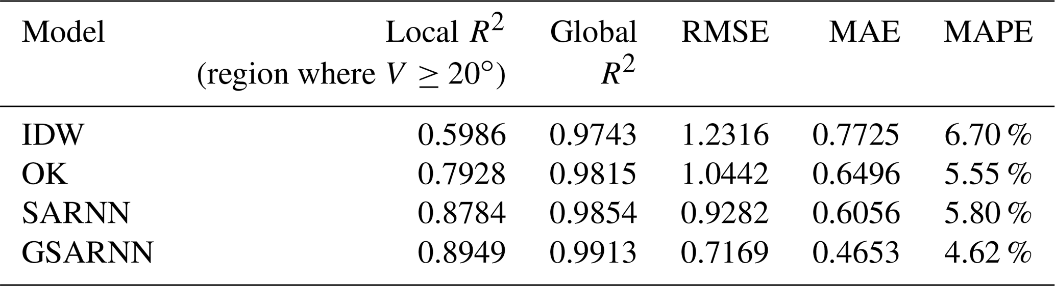
Figure 10 shows three-dimensional diagrams of the cross-validation interpolation results generated by the four methods and their corresponding interpolation errors. In interpolation error diagrams, red represents overestimation and blue represents underestimation. Taking the real dataset in Fig. 9 as a reference, the four models restore the data features in most areas, which is consistent with the statistical indicator results, with small differences in some details. The IDW method evidently underestimates the temperature at shallow depths, which may be because its interpolation mechanism can produce large errors at the edge points of a given space. In the OK results, the coexistence of underestimation and overestimation around the sea surface is observed, indicating that the OK method also has some limitations in edge-area interpolation. The SARNN and GSARNN models slightly overestimate the temperature of the bottom area. The error of GSARNN is generally smaller than that of SARNN. Further quantitative analysis is needed to elucidate more details of the interpolation experiment results.

Figure 10Three-dimensional diagrams of the cross-validation interpolation results and interpolation errors.
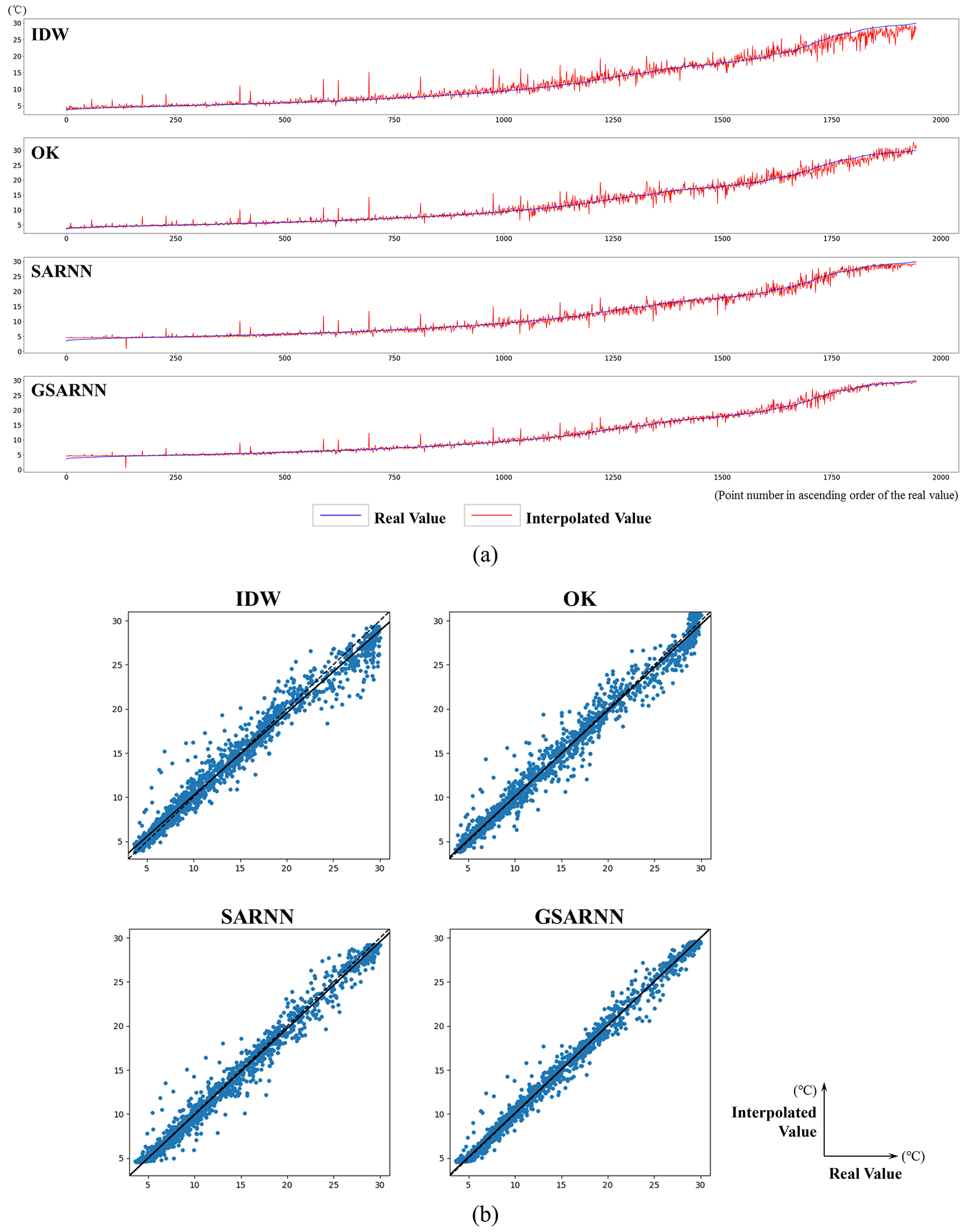
Figure 11The quantitative analysis results of the four models. (a) Line charts in ascending order of real value; (b) scatter diagrams with trend lines.
The cross-validation interpolation result values of the four models and the real values are respectively drawn as line charts and scatter diagrams, as shown in Fig. 11a and b. In the low-value area, the fluctuations of the four models are generally small. Several points with large errors are in similar positions for all models, indicating the presence of potential outliers in the dataset; however, the GSARNN model has the strongest ability to minimize these errors. In addition, the IDW, SARNN, and GSARNN methods marginally overestimate the lowest value. Entering the median area, the fluctuation of the four models begins to increase gradually; IDW produces the highest amplitude, followed in descending order by the OK, SARNN, and GSARNN methods. The GSARNN method avoids potential large errors in several positions to the greatest extent. In the high-value area, there are significant performance differences among the four models. The IDW method underestimates the high values across a large range, the SARNN model slightly underestimates them, the OK method fluctuates around the real values, and the GSARNN model hovers within a narrow range. The information conveyed by the scatter diagrams is consistent with the line charts. The scatter diagrams show that the scatter points of all four methods are concentrated around the diagonal, and the trend lines almost coincide with the standard trend line. Among them, the performance of the GSARNN is quantitatively best.
To compare the visual performance and effects of the four methods for practical interpolation applications, we interpolate and render horizontal sections at 100 m depth intervals in this area. Each method generates nine sections of 0–800 m depth, as shown in Fig. 12. The four methods produce similar interpolation results on the overall pattern, but there are great differences in detail. Due to the sparsity of the sampled points, the points closer to the section have a more prominent impact than the distant points in the interpolation results of the IDW method, producing many noticeable speckles on the interpolation surface. The OK method uses the statistical calculation process to fit the spatial features to a certain extent, alleviating the speckle problem; however, uneven color bands with abrupt color changes can still be observed. The SARNN and GSARNN models fit the continuous temperature field characteristics using the same set of sparse Argo temperature data. The overall change trend of the interpolated sections is consistent with the traditional methods but is significantly smoother and more uniform, reflecting the actual temperature field characteristics. Compared with the SARNN, the GSARNN presents richer details on the basis of smoothness, more exhaustively describing the ocean temperature field characteristics, showing the qualitatively best performance.
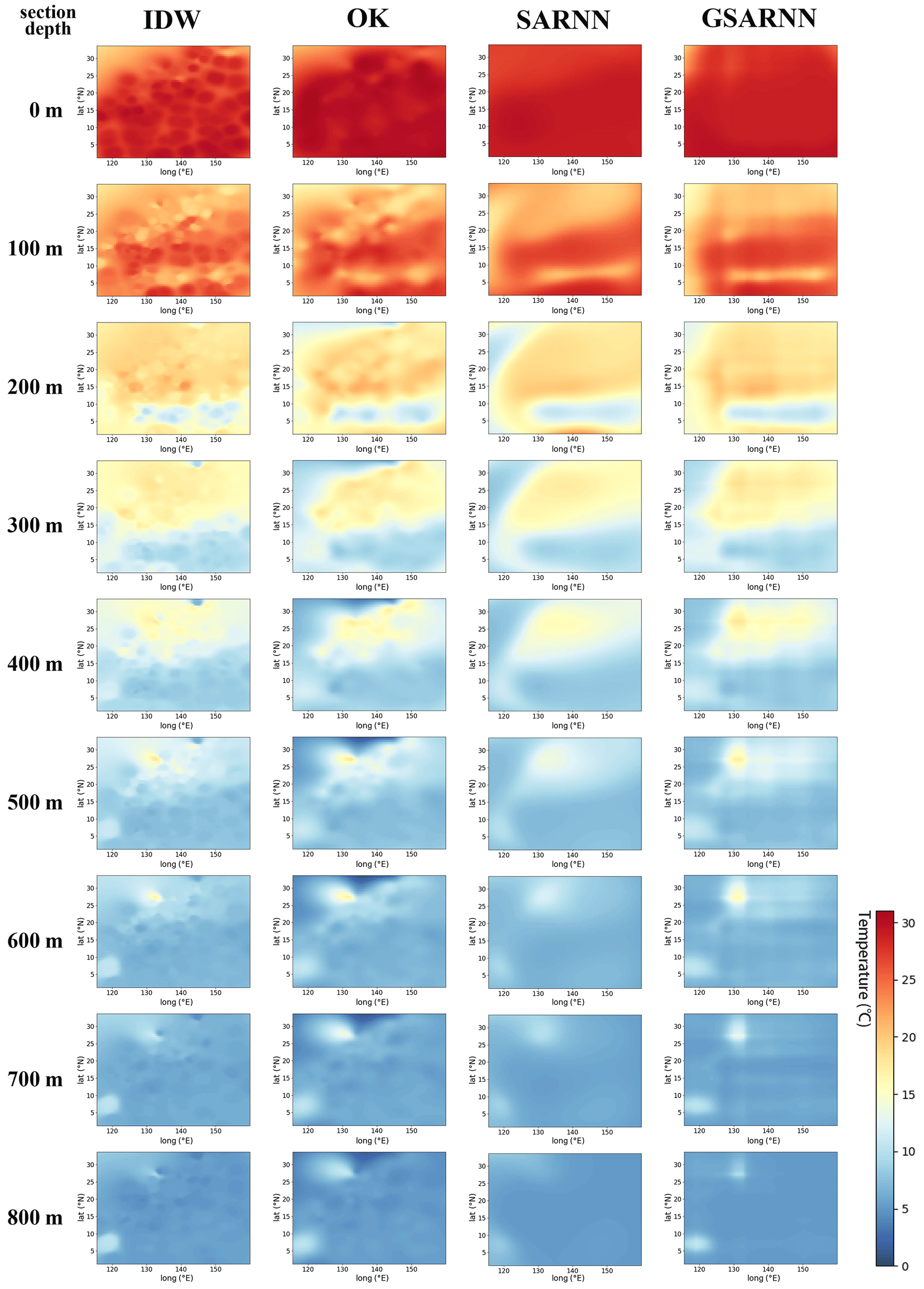
Figure 12Comparisons of interpolated horizontal sections at 100 m depth intervals generated by the four methods.
In case one, the comparison between two traditional interpolation methods and two neural-network-based methods demonstrates that introducing neural networks for powerful nonlinear fitting improves interpolation performance, enabling the adequate extraction and construction of complex change characteristics of spatial elements such as mutation. The comparison of the SARNN and GSARNN models shows that deconstructing and remodeling the expression and solution of spatial distances, and subsequently applying the generalized expression in interpolation calculations, enables the model to mine and restore the characteristics of the original data to the greatest extent, effectively improving the interpolation accuracy and optimizing the interpolation result.
In case two, the section interpolation prediction performance of the four methods varies considerably. The spatial distribution of the Argo buoys is sparse, uneven, and irregular, which is common in most practical interpolation scenarios. When interpolating such datasets, the traditional methods tend to produce dominant weights on the points adjacent to the point to be interpolated, which may lead to disproportionate regional impacts of specific sample points around them, resulting in uneven speckles and bands. Traditional methods lack the global consideration of the comprehensive effect of all sample points on the interpolation area. In contrast, neural-network-based models generate a smoother interpolation surface than traditional methods. This indicates that neural-network-based models can greatly reduce the influence of local extreme points on points to be interpolated and acquire quite reasonable spatial patterns of geospatial elements exploiting the non-linear fitting ability of neural networks. In particular, the GSARNN model incorporates the raw coordinate vectors as the network input and fits the generalized spatial distances in the three-dimensional spatial element field, extracting more detailed data features, generating interpolation results that are more consistent with reality.
In summary, in case one, we test the quantitative interpolation performance of the four methods on a dataset with complex characteristics; in case two, we examine the qualitative performance of the four methods in a practical interpolation application. The experiment results indicate that traditional methods are sensitive and dependent on the spatial distribution and data characteristics of the sampled points. By applying the concepts of neural networks, spatial autoregression, and generalized spatial distances to three-dimensional spatial interpolations, the GSARNN model can effectively optimize the interpolation result and improve the adaptability of interpolation methods in various scenarios.
In this study, we focus on the integration of interpolation and neural network model in three-dimensional space, in which the spatial elements possess complex characteristics. To improve the interpolation effect, we remodel the expression and solution of spatial distances and spatial weights – two critical elements in spatial interpolation. For spatial distance, we employ the generalized spatial distance expression and propose a GSDNN unit to adaptively generate the generalized spatial distance, replacing the conventional Euclidean spatial distance as the interpolation network input. For spatial weight, we construct the GSARNN model by integrating the GSDNN unit into the SARNN model. Exploiting the powerful feature extraction and nonlinear fitting abilities of neural networks, we can realize accurate spatial weight calculations.
Experiments are conducted on two three-dimensional cases: a simulated case and a real Argo temperature case. The GSARNN model is compared with the traditional IDW and OK methods and the advanced SARNN model. The experiment results indicate that the GSARNN model achieves the best interpolation performance among the four methods, especially on the complex three-dimensional spatial dataset with discontinuous features and sparse and irregular distribution. The GSARNN model can effectively extract subtle spatial correlation characteristics and accurately fit the spatial weights, adapting well in three-dimensional space.
The GSARNN can perform spatial interpolation with high accuracy at the cost of longer model training and calculation time. Therefore, the GSARNN is more suitable for interpolation scenarios with complex characteristics and strict demands on the result quality. For interpolation tasks with relatively simple spatial characteristics and specific requirements for efficiency, traditional methods may be a better choice.
In the future, we plan to consider the time dimension in addition to the spatial dimension to develop an accurate spatiotemporal data interpolation model. Meanwhile, based on the interpolation-dependent variable, the relevant regression variable factors can be introduced for further interpolation statistical analyses. In addition, as the number of sampled points increases, the number of input neurons and output neurons of the GSARNN will also increase, resulting in the expansion of network parameters and the extension of training time inevitably. Therefore, how to maintain a stable and acceptable training time given different sample data volumes is an important problem to be tackled in further research.
Simulated data, Argo temperature data, and codes used in the study are available at https://doi.org/10.6084/m9.figshare.18739571.v1 (Zhan and Wu, 2023).
JuZ, SW, JiZ, and ZD developed the model. JuZ, SW, and JQ implemented the model and conducted the experiments. JuZ, SW, MQ, and YW contributed to the planning and discussions and to the writing of the article.
The contact author has declared that none of the authors has any competing interests.
Publisher's note: Copernicus Publications remains neutral with regard to jurisdictional claims in published maps and institutional affiliations.
This work was supported by the National Natural Science Foundation of China (nos. 41922043, 41871287, and 42001323), the National Key Research and Development Program of China (nos. 2021YFB3900902 and 2018YFB0505000), and the Provincial Key R&D Program of Zhejiang (no. 2021C01031).
This paper was edited by Rohitash Chandra and reviewed by Chao Ma and three anonymous referees.
Abd El-Hady, A. E.-N. M., Abdelaty, E. F., and Salama, A. E.: GIS-mapping of soil available plant nutrients (potentiality, gradient, anisotropy), OJSS, 8, 315–329, https://doi.org/10.4236/ojss.2018.812023, 2018.
Adhikary, S. K., Muttil, N., and Yilmaz, A. G.: Cokriging for enhanced spatial interpolation of rainfall in two Australian catchments, Hydrol. Process., 31, 2143–2161, https://doi.org/10.1002/hyp.11163, 2017.
Allard, D., Senoussi, R., and Porcu, E.: Anisotropy models for spatial data, Math. Geosci., 48, 305–328, https://doi.org/10.1007/s11004-015-9594-x, 2016.
Arowolo, A. O., Bhowmik, A. K., Qi, W., and Deng, X.: Comparison of spatial interpolation techniques to generate high-resolution climate surfaces for Nigeria, Int. J. Climatol, 37, 179–192, https://doi.org/10.1002/joc.4990, 2017.
Aumond, P., Can, A., Mallet, V., De Coensel, B., Ribeiro, C., Botteldooren, D., and Lavandier, C.: Kriging-based spatial interpolation from measurements for sound level mapping in urban areas, J. Acoust. Soc. Am., 143, 2847–2857, https://doi.org/10.1121/1.5034799, 2018.
Babak, O. and Deutsch, C. V.: Statistical approach to inverse distance interpolation, Stoch. Environ. Res. Risk. Assess., 23, 543–553, https://doi.org/10.1007/s00477-008-0226-6, 2009.
Chen, D., Tian, Y., Yao, T., and Ou, T.: Satellite measurements reveal strong anisotropy in spatial coherence of climate variations over the Tibet Plateau, Sci. Rep., 6, 30304, https://doi.org/10.1038/srep30304, 2016.
Cheng, M., Wang, Y., Engel, B., Zhang, W., Peng, H., Chen, X., and Xia, H.: Performance assessment of spatial interpolation of precipitation for hydrological process simulation in the Three Gorges Basin, Water, 9, 838, https://doi.org/10.3390/w9110838, 2017.
da Silva Júnior, J. C., Medeiros, V., Garrozi, C., Montenegro, A., and Gonçalves, G. E.: Random forest techniques for spatial interpolation of evapotranspiration data from Brazilian's Northeast, Comput. Electron. Agr., 166, 105017, https://doi.org/10.1016/j.compag.2019.105017, 2019.
Du, Z., Wang, Z., Wu, S., Zhang, F., and Liu, R.: Geographically neural network weighted regression for the accurate estimation of spatial non-stationarity, Int. J. Geogr. Inf. Sci., 34, 1353–1377, https://doi.org/10.1080/13658816.2019.1707834, 2020.
Gao, B., Hu, M., Wang, J., Xu, C., Chen, Z., Fan, H., and Ding, H.: Spatial interpolation of marine environment data using P-MSN, Int. J. Geogr. Inf. Sci., 34, 577–603, https://doi.org/10.1080/13658816.2019.1683183, 2020.
Greenberg, J. A., Rueda, C., Hestir, E. L., Santos, M. J., and Ustin, S. L.: Least cost distance analysis for spatial interpolation, Comput. Geosci., 37, 272–276, https://doi.org/10.1016/j.cageo.2010.05.012, 2011.
He, K., Zhang, X., Ren, S., and Sun, J.: Delving deep into rectifiers: surpassing human-level performance on ImageNet classification, in: 2015 IEEE International Conference on Computer Vision (ICCV), Santiago, Chile, 1026–1034, https://doi.org/10.1109/ICCV.2015.123, 2015.
Hu, S., Cheng, Q., Wang, L., and Xu, D.: Modeling land price distribution using multifractal IDW interpolation and fractal filtering method, Landscape Urban Plan., 110, 25–35, https://doi.org/10.1016/j.landurbplan.2012.09.008, 2013.
Ioffe, S. and Szegedy, C.: Batch normalization: accelerating deep network training by reducing internal covariate shift, in: Proceedings of the 32nd International Conference on International Conference on Machine Learning – Volume 37, Lille, France, 448–456, https://doi.org/10.48550/arXiv.1502.03167, 2015.
Jian, Z. and Jin, H.: Ocean carbon cycle and tropical forcing of climate evolution, Adv. Earth Sci., 23, 221–227, https://doi.org/10.11867/j.issn.1001-8166.2008.03.0221, 2008.
Kanevski, M., Timonin, V., and Pozdnoukhov, A.: Automatic Decision-Oriented Mapping of Pollution Data, in: Computational Science and Its Applications – ICCSA 2008, edited by: Gervasi, O., Murgante, B., Laganà, A., Taniar, D., Mun, Y., and Gavrilova, M. L., Springer Berlin Heidelberg, Berlin, Heidelberg, vol. 5072, 678–691, https://doi.org/10.1007/978-3-540-69839-5_50, 2008.
Krige, D. G.: A statistical approach to some basic mine valuation problems on the Witwatersrand, Journal of the Chemical, Metallurgical and Mining Society of South Africa, 53, 159–162, 1952.
Kumar, S., Lal, R., and Liu, D.: A geographically weighted regression kriging approach for mapping soil organic carbon stock, Geoderma, 189–190, 627–634, https://doi.org/10.1016/j.geoderma.2012.05.022, 2012.
Li, C., Liu, Y., Wu, J., Wang, C., and Liu, X.: A contrastive study on the spatial interpolation for precipitation data using back propagation learning algorithm and support vector machine model – a case study of Gansu Province, Grassland and Turf, 38, 12–19, https://doi.org/10.13817/j.cnki.cyycp.2018.04.002, 2018.
Li, Z., Zhang, X., Zhu, R., Zhang, Z., and Weng, Z.: Integrating data-to-data correlation into inverse distance weighting, Comput. Geosci., 24, 203–216, https://doi.org/10.1007/s10596-019-09913-9, 2020.
Liang, Q., Nittel, S., Whittier, J. C., and Bruin, S.: Real-time inverse distance weighting interpolation for streaming sensor data, Trans. GIS, 22, 1179–1204, https://doi.org/10.1111/tgis.12458, 2018.
Liu, Z., Wu, X., Xu, J., Li, H., Lu, S., Sun, C., and Cao, M.: China Argo project: progress in China Argo ocean observations and data applications, Acta Oceanol. Sin., 36, 1–11, https://doi.org/10.1007/s13131-017-1035-x, 2017.
Longley, P. A., Goodchild, M., Maguire, D. J., and Rhind, D. W. (Eds.): Geographic information systems & science, 3rd Edn., Wiley, Hoboken, NJ, 539 pp., ISBN 978-0-470-72144-5, 2011.
Lu, G. Y. and Wong, D. W.: An adaptive inverse-distance weighting spatial interpolation technique, Comput. Geosci., 34, 1044–1055, https://doi.org/10.1016/j.cageo.2007.07.010, 2008.
Ma, X., Luan, S., Ding, C., Liu, H., and Wang, Y.: Spatial interpolation of missing annual average daily traffic data using Copula-based model, IEEE Intell. Transp. Sy., 11, 158–170, https://doi.org/10.1109/MITS.2019.2919504, 2019.
Matheron, G.: Principles of geostatistics, Econ. Geol., 58, 1246–1266, https://doi.org/10.2113/gsecongeo.58.8.1246, 1963.
Pan, S., Tian, S., Wang, X., Dai, L., Gao, C., and Tong, J.: Comparing different spatial interpolation methods to predict the distribution of fishes: a case study from Coilia nasus in the Changjiang River Estuary, Acta Oceanol. Sin., 40, 1–14, https://doi.org/10.1007/s13131-021-1789-z, 2021.
Rigol, J. P., Jarvis, C. H., and Stuart, N.: Artificial neural networks as a tool for spatial interpolation, Int. J. Geogr. Inf. Sci., 15, 323–343, https://doi.org/10.1080/13658810110038951, 2001.
Riser, S. C., Freeland, H. J., Roemmich, D., Wijffels, S., Troisi, A., Belbéoch, M., Gilbert, D., Xu, J., Pouliquen, S., Thresher, A., Le Traon, P.-Y., Maze, G., Klein, B., Ravichandran, M., Grant, F., Poulain, P.-M., Suga, T., Lim, B., Sterl, A., Sutton, P., Mork, K.-A., Vélez-Belchí, P. J., Ansorge, I., King, B., Turton, J., Baringer, M., and Jayne, S. R.: Fifteen years of ocean observations with the global Argo array, Nat. Clim. Change, 6, 145–153, https://doi.org/10.1038/nclimate2872, 2016.
Samal, A. R., Sengupta, R. R., and Fifarek, R. H.: Modelling spatial anisotropy of gold concentration data using GIS-based interpolated maps and variogram analysis: Implications for structural control of mineralization, J. Earth Syst. Sci., 120, 583–593, https://doi.org/10.1007/s12040-011-0091-4, 2011.
Sekulić, A., Kilibarda, M., Heuvelink, G. B. M., Nikolić, M., and Bajat, B.: Random Forest Spatial Interpolation, Remote Sensing, 12, 1687, https://doi.org/10.3390/rs12101687, 2020.
Shepard, D.: A two-dimensional interpolation function for irregularly-spaced data, in: Proceedings of the 1968 23rd ACM national conference, the 1968 23rd ACM National Conference, New York, NY, US, 517–524, https://doi.org/10.1145/800186.810616, 1968.
Srivastava, N., Hinton, G., Krizhevsky, A., Sutskever, I., and Salakhutdinov, R.: Dropout: a simple way to prevent neural networks from overfitting, J. Mach. Learn. Res., 15, 1929–1958, https://dl.acm.org/doi/10.5555/2627435.2670313, 2014.
Sun, M., Liu, S., and Liu, J.: IDW interpolation algorithm considering spatial anisotropy, Computer Engineering and Design, 41, 983–987, https://doi.org/10.16208/j.issn1000-7024.2020.04.014, 2020.
Szczepańska, A., Gościewski, D., and Gerus-Gościewska, M.: A GRID-based spatial interpolation method as a tool supporting real estate market analyses, IJGI, 9, 39, https://doi.org/10.3390/ijgi9010039, 2020.
Tamura, S. and Tateishi, M.: Capabilities of a four-layered feedforward neural network: four layers versus three, IEEE T. Neural Networ., 8, 251–255, https://doi.org/10.1109/72.557662, 1997.
Tang, M., Wu, X., Agrawal, P., Pongpaichet, S., and Jain, R.: Integration of diverse data sources for spatial PM2.5 data interpolation, IEEE T. Multimedia, 19, 408–417, https://doi.org/10.1109/TMM.2016.2613639, 2017.
Tao, H., Liao, X., Zhao, D., Gong, X., and Cassidy, D. P.: Delineation of soil contaminant plumes at a co-contaminated site using BP neural networks and geostatistics, Geoderma, 354, 113878, https://doi.org/10.1016/j.geoderma.2019.07.036, 2019.
Tobler, W. R.: A computer movie simulating urban growth in the Detroit region, Econ. Geogr., 46, 234–240, https://doi.org/10.2307/143141, 1970.
Wang, D., Chen, Y., and Zhan, W.: A geometric model to simulate thermal anisotropy over a sparse urban surface (GUTA-sparse), Remote Sens. Environ., 209, 263–274, https://doi.org/10.1016/j.rse.2018.02.051, 2018.
Wang, Q.: The fast three-dimentional kriging interpolation method based on Delaunay, ME thesis, University of Electronic Science and Technology of China, China, 71 pp., 2015.
Watson, D. F. and Philip, G. M.: A refinement of inverse distance weighted interpolation, Geoprocessing, 2, 315–327, https://doi.org/10.1016/S0735-1097(97)00186-1, 1985.
Wu, S., Du, Z., Wang, Y., Lin, T., Zhang, F., and Liu, R.: Modeling spatially anisotropic nonstationary processes in coastal environments based on a directional geographically neural network weighted regression, Sci. Total Environ., 709, 136097, https://doi.org/10.1016/j.scitotenv.2019.136097, 2020.
Zeng, J., Zhang, F., Wu, S., Du, Z., and Liu, R.: Spatial interpolation based on spatial auto-regressive neural network, Journal of Zhejiang University (Science Edition), 47, 572–581, https://doi.org/10.3785/j.issn.1008-9497.2020.05.009, 2020.
Zhan, J. and Wu, S.: GSARNN Code and Data, figshare [data set], https://doi.org/10.6084/m9.figshare.18739571.v1, 2023.
Zhang, X., Liu, G., Wang, H., and Li, X.: Application of a Hybrid Interpolation Method Based on Support Vector Machine in the Precipitation Spatial Interpolation of Basins, Water, 9, 760, https://doi.org/10.3390/w9100760, 2017.
Zhang, Y., Hidalgo, J., and Parker, D.: Impact of variability and anisotropy in the correlation decay distance for precipitation spatial interpolation in China, Clim. Res., 74, 81–93, https://doi.org/10.3354/cr01486, 2017.
Zhang, Y., Feng, M., Zhang, W., Wang, H., and Wang, P.: A Gaussian process regression-based sea surface temperature interpolation algorithm, J. Ocean. Limnol., 39, 1211–1221, https://doi.org/10.1007/s00343-020-0062-1, 2021.