CLGAN: a generative adversarial network (GAN)-based video prediction model for precipitation nowcasting

The prediction of precipitation patterns up to 2 h ahead, also known as precipitation nowcasting, at high spatiotemporal resolutions is of great relevance in weather-dependent decision-making and early warning systems. In this study, we are aiming to provide an efficient and easy-to-understand deep neural network – CLGAN (convolutional long short-term memory generative adversarial network) – to improve the nowcasting skills of heavy precipitation events. The model constitutes a generative adversarial network (GAN) architecture, whose generator is built upon a u-shaped encoder–decoder network (U-Net) and is equipped with recurrent long short-term memory (LSTM) cells to capture spatiotemporal features. The optical flow model DenseRotation and the competitive video prediction models ConvLSTM (convolutional LSTM) and PredRNN-v2 (predictive recurrent neural network version 2) are used as the competitors. A series of evaluation metrics, including the root mean square error, the critical success index, the fractions skill score, and object-based diagnostic evaluation, are utilized for a comprehensive comparison against competing baseline models. We show that CLGAN outperforms the competitors in terms of scores for dichotomous events and object-based diagnostics. A sensitivity analysis on the weight of the GAN component indicates that the GAN-based architecture helps to capture heavy precipitation events. The results encourage future work based on the proposed CLGAN architecture to improve the precipitation nowcasting and early warning systems.

1 Introduction

Heavy precipitation can lead to numerous hazards, cause damage to infrastructure, and even increase risk to human life (Ganguly and Bras, 2003; Vasiloff et al., 2007; Li et al., 2021). Accurate short-term predictions of precipitation events at high spatiotemporal resolutions, also known as precipitation nowcasting, are therefore critical in establishing early warning systems. These warning systems can in turn help authorities in weather-dependent decision-making and enhance risk-governance capabilities (Dixon and Wiener, 1993; Johnson et al., 1998; Bowler et al., 2006).

Current precipitation nowcasting systems mainly rely on convective-permitting numeric weather prediction (NWP) or on extrapolation techniques of precipitation patterns with the help of composite radar observations. However, NWP models suffer from difficulties in capturing these patterns in the nowcasting time range due to the spin-up effect and the challenges of handling non-Gaussian data in assimilation (Ravuri et al., 2021). Also, a quick model run cycle would be required. For instance, ICON-D2 only initializes every 3 h (Matsunobu et al., 2022), which makes it impossible to get quick updates in light of rapidly growing precipitation patterns. Observation-based extrapolation methods, such as optical flow, are commonly superior to NWP models for precipitation nowcasting but also fail to capture the underlying nonlinear processes of precipitation formation, e.g., secondary triggering and aggregation (Xie et al., 2019).

Deep neural networks have gained increasing attention in the meteorological community over the last few years (Reichstein et al., 2019; Schultz et al., 2021). The growing interest can be attributed to the success stories in other domains where deep learning (DL) has been proven to leverage high-level information from complex and highly nonlinear data in several applications, such as autonomous driving (Hu et al., 2020), anomaly detection (Liu et al., 2018), and semantic segmentation (Garcia-Garcia et al., 2018). Recently, video prediction models, developed in the computer vision community, have been explored for precipitation nowcasting. Contemporary studies mainly applied model architectures based on u-shaped convolutional networks (U-Net; e.g., Ayzel et al., 2020; Ronneberger et al., 2015), convolutional long short-term memory cells (ConvLSTM; e.g., Shi et al., 2015), and generative (see, e.g., Ravuri et al., 2021) and attention models (see, e.g., Sønderby et al., 2020). U-Nets are thereby considered to be beneficial since they are capable of extracting multi-scale features of the atmospheric processes (Ronneberger et al., 2015). To also explicitly capture temporal dependencies in the underlying formation process of precipitation, recurrent ConvLSTM models are an appealing choice (Shi et al., 2015). Thus, combining convolutional and recurrent networks with ConvLSTM layers is advantageous in generating stable precipitation nowcasting by encoding the spatial and temporal dependencies from the historical frames.

Nevertheless, these models have problems with handling the statistical nature of precipitation, especially when a pixel-wise loss function is applied for the optimization process during training (Shi et al., 2017; Ayzel et al., 2020). Although log transformation, importance sampling, and weighting towards heavier precipitation targets are appropriate to govern the right-skewed gamma distribution of precipitation rates (e.g., Ravuri et al., 2021), the inherent uncertainty in quasi-chaotic processes at mesoscale typically leads to unrealistically smooth precipitation patterns in the forecasts. While this issue is well known in many other video prediction tasks (Mathieu et al., 2015; Ebert et al., 2017), it is of particular relevance in precipitation nowcasting. The high spatiotemporal variability seen in the observational (real) data cannot be maintained, and thus, heavy precipitation events are barely captured by models applying a pixel-wise loss. Generative models, which train a generator and a discriminator adversarially (generative adversarial network – GAN – models) are considered to be a potential solution for such applications (Goodfellow et al., 2020). By forcing the generator to fool the discriminator, which aims to distinguish between real and generated data, these models succeed in maintaining the statistical properties of the underlying data (Oprea et al., 2020).

Although great progress has been achieved in a series of recent studies (e.g., Ravuri et al., 2021; Gong et al., 2022), there is controversy regarding how different components of sophisticated model architectures contribute to the predictions. Motivated by this, we build a simple but efficient and easy-to-understand video prediction model, CLGAN (convolutional long short-term memory generative adversarial network; see Fig. 1), for the nowcasting task. CLGAN is proposed to leverage the advantages of different DL model architectures. The generator combines the U-Net with a ConvLSTM cell to abstract spatial features on multiple scales, while the temporal dependency of precipitation patterns is also preserved. The generator network is then trained adversarially to attain precipitation forecasts resembling observed data. For our nowcasting application, we deploy a gridded dataset with a temporal resolution of 10 min aggregated from automatic weather station (AWS) gauges over Guizhou, China. The predictive performance of the proposed model architecture is then accessed in a comprehensive evaluation based on metrics designed for precipitation nowcasting. The evaluation also involves a comparison against a simplistic persistence forecast, the conventional optical flow model DenseRotation (Ayzel et al., 2019), as well as two baseline video prediction models, a standard ConvLSTM (Shi et al., 2015) network and an up-to-date competing model PredRNN-v2 (predictive recurrent neural network version 2) (Wang et al., 2021).

With this, the main contributions of our study are as follows.

• An efficient and easy-to-understand architecture, CLGAN, leveraging the merits of U-Net, ConvLSTM, and GAN models is proposed to generate perceptually realistic precipitation forecasts.

• A new 10 min level precipitation dataset based on AWS gauges (Guizhou AWS_ML precipitation dataset) is built for machine learning experiments.

• Nowcasting of heavy precipitation events is improved with comprehensive verification.

• A sensitivity analysis is performed to assess the importance of adversarial training for generating forecasts with closer statistical properties of the observed precipitation.

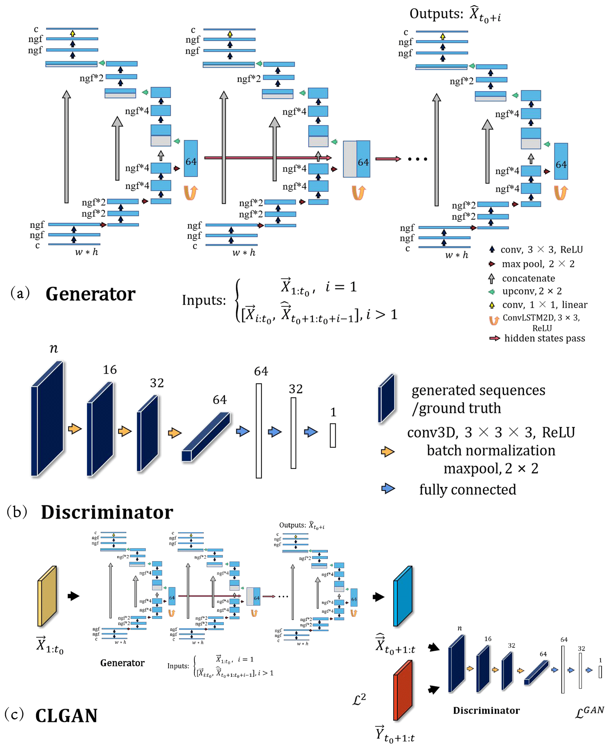
Figure 1 The details of the proposed CLGAN model. (a) Generator: the illustration is presented for a given forecast step i. If i=1, the inputs are observed sequences ${\mathit{X}}_{\mathrm{1}:t_{\mathrm{0}}}$. Otherwise the inputs are combined sequences of observed ones ${\mathit{X}}_{i:t_{\mathrm{0}}}$ and predicted ones ${\widehat{\mathit{X}}}_{t_{\mathrm{0}}+\mathrm{1}:t_{\mathrm{0}}+i-\mathrm{1}}$. The output is the model prediction ${\widehat{\mathit{X}}}_{t_{\mathrm{0}}+i}$, c is the number of channels of inputs and here is 1, and ngf denotes the number of filters in the first layer of U-Net. (b) Discriminator: n is the length of output sequences. (c) CLGAN: the outputs of the generator are the predicted sequences ${\widehat{\mathit{X}}}_{t_{\mathrm{0}}+\mathrm{1}:t}$. ${\mathit{Y}}_{t_{\mathrm{0}}+\mathrm{1}:t}$ constitutes the corresponding ground truth. ℒ² and ℒ^GAN are the reconstruction loss and adversarial loss, respectively.

2 Related work and baseline models

2.1 Conventional methods

The simplest approach to generate precipitation “forecasts” is to deploy the Eulerian persistence. For this, the most recent available observation, usually a radar composite, is used and then replicated several times for the future steps. This approach is quite accurate for very short lead times but obviously fails to provide meaningful forecasts in a quickly evolving system for timescales beyond several minutes such as the atmosphere. Thus, the related forecast quality can be considered as the minimum level for a prediction model to be useful.

Conventional precipitation nowcasting systems typically use a Lagrangian framework to predict the development of precipitation patterns. Although this framework often assumes the persistence of the precipitation features' intensity and displacement, it is still capable of outperforming mesoscale NWP models in precipitation nowcasting (Sun et al., 2014). The Lagrangian method applies a two-step approach where the precipitation features are first tracked and then extrapolated to future time steps (Austin and Bellon, 1974). Typically, the tracking step is accomplished with the help of optical flow methods that infer the motion of patterns from consecutive images. For precipitation nowcasting, radar composite images are subject to a tracking algorithm such as cross-correlation tracking (Rinehart and Garvey, 1978; Grecu and Krajewski, 2000; Zahraei et al., 2012) or centroid tracking techniques (Zahraei et al., 2013). The tracked objects are then applied to different extrapolation schemes, e.g., image warping (Wolberg, 1990), constant-vector advection (Bowler et al., 2004), or semi-Lagrangian schemes (Germann and Zawadzki, 2002). With this two-step approach, several operational precipitation nowcasting systems have been established over the globe in the last 3 decades, such as the Thunderstorm Identification Tracking Nowcasting (TITAN; Dixon and Wiener, 1993), the Storm Cell Identification and Tracking (SCIT; Johnson et al., 1998), and the Short‐Term Ensemble Prediction System (STEPS; Bowler et al., 2006) (see Wilson et al., 2010, for a review on operational systems).

Recently, Ayzel et al. (2019) implemented a set of advanced optical flow models into an open-source Python library called rainymotion. Two different groups of methods are part of this library from which we select the DenseRotation model that performs best in their study. The tracking algorithm of this model is based on the dense inverse search algorithm proposed in Kroeger et al. (2016) providing an estimate of the motion of each pixel based on two consecutive radar images. The extrapolation is then performed with a semi-Lagrangian advection scheme (Germann and Zawadzki, 2002) capable of representing rotational motions.

In our study, the Eulerian persistence model and the DenseRotation model are used to show how well the traditional methods can perform for the precipitation nowcasting task and how much benefit can be further obtained by using DL-based video prediction methods.

2.2 Video prediction method

As already mentioned, the application of deep learning techniques in the meteorological community has gained momentum over the recent years. In particular, several studies have started to explore these techniques to tackle the precipitation nowcasting problem. By formulating precipitation nowcasting as a sequence prediction task, Shi et al. (2015) proposed a network of ConvLSTM cells which apply a convolution in the recurrent layers of the vanilla LSTM to capture spatiotemporal features in the underlying data. Their two-layer ConvLSTM network was able to outperform the Variational Methods for Echoes of Radar (ROVER) by Woo and Wong (2017), an operational precipitation nowcasting system based on optical flow methods with a semi-Lagrangian advection scheme. Shi et al. (2017) further extended the recurrent cells of gated recurrent units (GRUs) with non-local neural connections and proposed the Trajectory GRU (TrajGRU) model which enables the learning of location-variant structures of precipitation.

Besides, Wang et al. (2017) advanced the application of ConvLSTM networks and proposed the predictive recurrent neural network (PredRNN). They deployed a stack of recurrent layers that feature a “zigzag memory flow” and involve an explicit spatiotemporal memory state. In this way, they enable an explicit communication of abstracted spatiotemporal features between different levels of the recurrent network which yields improved precipitation predictions. While this approach already provided promising results, the PredRNN model was updated to PredRNN-v2 (Wang et al., 2021). The updates comprise the implementation of a “decoupling loss”, named ST-LSTM, to enhance the featuring of the spatiotemporal variations and a new, improved long-term modeling strategy. The model attains remarkable improvements when applied to multiple datasets including radar observations.

Meanwhile, other network architectures were explored in the scope of precipitation nowcasting. One of them is the fully convolutional U-Net architecture, which is a u-shaped hierarchical encoder–decoder network with skip connections. The architecture enables the abstraction of features on different spatial scales. Notably, the RainNet architecture proposed by Ayzel et al. (2020) proved to significantly outperform optical-flow-based nowcasting methods for weak precipitation events. However, their network tends to provide too smooth precipitation fields and therefore fails to provide added value for more intense precipitation events with a rain rate above 10 mm h⁻¹. Recently, a deep generative model for the probabilistic precipitation nowcasting was proposed and showed state-of-the-art performance for the task (Ravuri et al., 2021).

All these studies demonstrate that deep neural networks have the potential to provide added value for precipitation nowcasting. In our study, we focus on further improving the predictions of strong precipitation events and therefore choose a simple ConvLSTM (Shi et al., 2015) and the advanced PredRNN-v2 (Wang et al., 2021) model for competing with our newly proposed model architecture.

3 Method and data

3.1 Our model CLGAN

In the following, we present our proposed CLGAN architecture in more detail. Since CLGAN aims to benefit from ConvLSTM models, the U-Net architecture, and GAN models, we first introduce its components separately to provide a deeper understanding of and reasoning for the chosen components.

3.1.1 ConvLSTM

The ConvLSTM network was proposed as an extension of LSTM layers which embedded the convolution operation to explicitly encode complex spatiotemporal features in a data sequence. The basic formulas of the ConvLSTM cell which describe the gated update procedure for the hidden and cell state are provided in Shi et al. (2015) and are therefore not repeated here. The objective function of a ConvLSTM model typically constitutes the classical ℒ² reconstruction loss. This loss measures the distance between the predicted and the target (ground truth) data on the grid-point (or pixel-wise) level and can be written as

$$\begin{array}{}\text{(1)}& {\mathcal{L}}^{\mathrm{2}}\left(G\right)={∥{\mathit{Y}}_{t_{\mathrm{0}}+\mathrm{1}:t}-{\widehat{\mathit{X}}}_{t_{\mathrm{0}}+\mathrm{1}:t}∥}_{\mathrm{2}},\end{array}$$

where Y and $\widehat{\mathit{X}}$ are 2D tensors for the ground truth and the predicted data, respectively. t₀ represents the end of the input sequence, and t is the forecast time step, so the model is optimized on the loss over the prediction sequence from t₀+1 to t. These tensors comprise w×h grid points in zonal and meridional directions of the domain of interest.

3.1.2 U-Net

The U-Net model was originally applied for biomedical image segmentation (Ronneberger et al., 2015) and is therefore designed as a powerful feature extractor on various spatial scales. As illustrated in Fig. 1a, it can be decomposed into a compressing and an expansive path that are bridged by skip connections. The contracting path can be seen as an encoder which converts the highly resolved data into coarse-grained features using convolutional and pooling layers. The expansive path, acting as a decoder, applies deconvolutional layers to convert back to the original spatial resolution, of which the number of data points are w×h. Usually, several pooling and deconvolutional layers are applied to allow feature extraction on different spatial scales. To avoid the so-called vanishing gradients issue and to allow a direct information flow of specific spatial features, skip connections are implemented at every scale-specific feature extraction level (Drozdzal et al., 2016).

In a video prediction application, the data at time step t enter the encoder to produce a forecast at time step t+1 with the decoder. By doing so, no long-term information is explicitly conveyed as with the ConvLSTM model. Since heavy precipitation events are rare but of high relevance for nowcasting, different techniques are usually applied to encourage deep neural networks in predicting events on the right tail of the underlying probability density function. Log transformation converts the right-skewed gamma distribution of precipitation data (e.g., RainNet in Ayzel et al., 2020) into a Gaussian-like distribution which puts strong precipitation events closer to the center of mass in probability space. Stronger weighting on higher precipitation rates and importance sampling can further support the optimization efficiency with respect to heavy precipitation events (Ravuri et al., 2021). Nonetheless, U-Nets and ConvLSTM modes still tend to produce too smooth precipitation patterns, thereby failing to capture the relevant strong precipitation events.

3.1.3 Generative adversarial networks

To enforce a closer agreement of the generated data with the ground truth, GAN models were proposed by Goodfellow et al. (2020). A GAN model consists of a generative network G (generator) and a discriminative network D (discriminator) which aims to assign a probability of 1 to real and a probability of 0 to generated data. While the discriminator is optimized to distinguish between both kinds of inputted data, the generator is encouraged to fool the discriminator. Thus, the GAN applies the binary cross-entropy loss as the objective function which enters a minimax game:

$$\begin{array}{}\text{(2)}& \begin{array}{rl}{G}^{\star }& =\arg \underset{G}{min}\underset{D}{max}{\mathcal{L}}^{\mathrm{GAN}}(G,D)\\ \text{with }& {\mathcal{L}}^{\mathrm{GAN}}(G,D)={\mathbb{E}}_{{\mathit{X}}_{\mathrm{1}:t}}\left[\log D\left({\mathit{X}}_{t_{\mathrm{0}}+\mathrm{1}:t}\right)\right]\\ & +{\mathbb{E}}_{{\mathit{X}}_{\mathrm{1}:t}}\left[\log (\mathrm{1}-D(G\left({\mathit{X}}_{\mathrm{1}:t_{\mathrm{0}}}\right)\left)\right)\right].\end{array}\end{array}$$

Here, the generator is conditioned on the input data sequence ${\mathit{X}}_{\mathrm{1}:t_{\mathrm{0}}}$. Since generator and discriminator are trained adversarially, the generator is encouraged to create predictions that share the same statistical properties as the ground truth data. This is considered to be useful for generating realistic precipitation forecasts which should exhibit the high spatial variability in the observed data (Ravuri et al., 2021; Price and Rasp, 2022; Harris et al., 2022).

3.1.4 Convolutional LSTM GAN (CLGAN)

To combine the merits of a GAN model with the strong spatiotemporal feature extraction capacities of U-Nets and ConvLSTM models, we set up the generator G as follows (see Fig. 1a). The generator constitutes a three-level U-Net following Sha et al. (2020). Each level of the encoder comprises two convolutional layers followed by max pooling with a 2×2 kernel to reduce the spatial dimensionality in the next layer. The number of channels is thereby increased by a factor of 2 in each level. A ConvLSTM cell with 64 filters is deployed to implement recurrency at the bridge between the encoder and decoder. The decoder then reverts the encoded data to the input resolution with the help of deconvolutional layers. Furthermore, skip connections among the encoder and decoder are added at each level of the U-Net. The discriminator D consists of 3D fully convolutional layers with batch normalization which allow us to encode both the temporal and spatial dimensions of the data sequence. Again, max pooling is used to compress the data which finally get concatenated to fully connected layers (see Fig. 1b). The forecast sequence of G, ${\widehat{\mathit{X}}}_{t_{\mathrm{0}}+\mathrm{1}:t}$, and the corresponding ground truth sequence, ${\mathit{Y}}_{t_{\mathrm{0}}+\mathrm{1}:t}$, are taken as the inputs for the discriminator D (see Fig. 1c).

In this study, the generator is trained by combining the adversarial loss ℒ^GAN with the reconstruction ℒ² loss:

$$\begin{array}{}\text{(3)}& G^{\star }=(\mathrm{1}-\mathit{\lambda }){\mathcal{L}}^{\mathrm{GAN}}(G,D)+\mathit{\lambda }{\mathcal{L}}^{\mathrm{2}}\left(G\right)\text{with }\mathit{\lambda }\in [\mathrm{0},\mathrm{1}].\end{array}$$

This ensures that the prediction remains close to the ground truth. The relative weight of the reconstruction loss λ is set to 0.99, which proves to balance the contributions from both loss components in the following experiments. Training of the model is performed with the Adam optimizer (Kingma and Ba, 2014) over eight epochs with a batch size of 32.

3.2 Guizhou AWS_ML precipitation dataset

In addition to the widely used remote sensing data, e.g., radar composite images, measurements from densely distributed automatic weather stations can serve as an alternative in the data-driven weather forecasting task. In this study, minute-level precipitation measurements by rain gauges of AWSs over Guizhou, China (Guizhou AWS_ML precipitation dataset), are collected for the precipitation nowcasting task. Guizhou is a mountainous and rainy province located in southwest China (see Fig. 2a) where mudslides happen frequently during summertime. For instance, the region was affected by a severe rainstorm in September 2020, in which some regions experienced more than 1500 mm rainfall within 20 d. Accurate precipitation nowcasting, especially for heavy precipitation, is crucial to reduce damage from these events. Hence, the Guizhou AWS_ML precipitation dataset is established for better simulation of precipitation with data-driven approaches. The AWS locations comprise 93 basic national stations and 1740 automatic weather stations (see Fig. 2b). Among other meteorological quantities (2 m temperature, 10 m wind, surface pressure, and relative humidity), the AWSs measure precipitation at a high observation frequency (every minute), and the data are provided between 1 January 2015 and 31 December 2019 by Guizhou Meteorological Bureau.

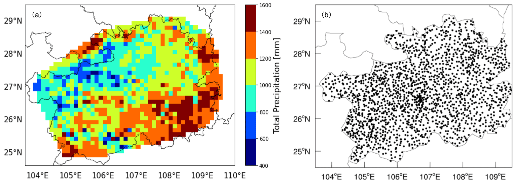
Figure 2 (a) Annual average cumulative precipitation in Guizhou from 2015 to 2019. (b) The spatial distribution of AWSs over Guizhou.

Several preprocessing steps are conducted for preparing the dataset of our experiment. First, the precipitation data are accumulated over 10 min, which still constitutes a reasonably high temporal resolution. To obtain a gridded dataset, the observations are then interpolated bilinearly onto a regular, spherical grid. The target grid comprises $w\times h=\mathrm{48}\times \mathrm{40}$ data points in zonal and meridional directions, respectively, and covers a domain from 24.625 to 29.5^∘ N and 103.625 to 109.5^∘ E with 0.125^∘ resolution. To obtain the data needed for training our CLGAN and the baseline models (see Sects. 2 and 3.1.4), we generate sliding sequences of 24 consecutive gridded data samples (frames) which comprise a temporal period of 240 min, and 120 min (12 frames) of each sequence serves as input to predict the next 120 min (12 frames). Since there are many periods with no or only weak precipitation, we furthermore only select sequences whose averaged precipitation rate exceeds the empirical 60 % quantile of the complete dataset. This results in 35 054 sequences for the subsampled dataset. Finally, a log transformation is applied to each sequence to make the data more Gaussian-like. The log transformation reads as follows: $x^{\prime }=\ln (x+\mathit{\epsilon })-\ln \left(\mathit{\epsilon }\right)$, where ε is a small constant (here 0.01). We use the data from 2015 to 2017 for training, the data of 2018 for validating, and the data of 2019 for testing.

3.3 Verification methods

As pointed out in Schultz et al. (2021) and more specifically for precipitation in Leinonen et al. (2020), precipitation nowcasting should be evaluated in terms of application-specific scores. This is due to the unique statistical properties of precipitation rates, as well as the chaotic atmospheric processes which underpin the formation of precipitation. Additionally, we would like to emphasize that a single score alone can barely evaluate the model performance applied to high-dimensional data (Wilks, 2011). Therefore, we take several evaluation metrics into account to provide a comprehensive overview.

The first considered family of evaluation metrics is established for continuous quantities in the meteorological community. The root mean square error (RMSE) measures the distance between the predicted and the observed field on a grid-point level. The correlation coefficient (CC) measures the association or the linear relationship between the two fields. A perfect correlation would result in CC=1, while CC=0 indicates no linear relationship between forecast and observation on the grid-point level.

The second set of scores is built on dichotomous events which are obtained by thresholding the gridded precipitation fields. A 2×2 contingency table is commonly used to show the frequency of “yes” and “no” forecasts and occurrences and give a joint distribution for events with a precipitation rate exceeding a given threshold t_pr. According to the elements in the contingency table, a variety of categorical statistics can be computed to evaluate the dichotomous forecasts in particular aspects. Critical success index (CSI), also known as threat score, measures the fraction of hits with respect to the number of occurrences where the events are either forecasted or observed. The frequently applied equitable threat score (ETS) is a variant of the CSI and explicitly accounts for random forecasts which perform well just by chance (Wilks, 2011).

However, due to the highly nonlinear and complex processes causing precipitation formation, scores acting on grid-point level are prone to penalize predictions which recover the high spatial variability but fail to match exactly the observed precipitation field. The issue leads to the double penalty problem where the model gets penalized twice, once for missing the exact placement of a precipitation event and once for shifting it spatially (Ebert, 2008). To relax the requirement for exact spatial matching, the fractions skill score (FSS) is computed here as a fuzzy verification metric (Roberts, 2008). Similar to the CSI and ETS, the FSS operates on dichotomous events but allows for spatial shifts by considering a local neighborhood around each grid point. Within this neighborhood, the fractional coverage of the precipitation events is calculated for both the predictions and the observations. Let $f\left(m_i^s\right)$ and $f\left(o_i^s\right)$ denote the fraction of event grid boxes within the local neighborhood of size s around the grid point i in the model prediction and observation. The fractions Brier score (FBS) is given by

$$\begin{array}{}\text{(4)}& \text{FBS}={\displaystyle \frac{\mathrm{1}}{N}}\sum _{i=\mathrm{1}}^N\left(f\right(m_i^s)-f(o_i^s){)}^{\mathrm{2}},\end{array}$$

which quantifies the quadratic difference between the prediction and the observation for all N grid points over the domain. The final FSS is then obtained with

$$\begin{array}{}\text{(5)}& \text{FSS}=\mathrm{1}-\text{FBS}/{\text{FBS}}_{\mathrm{worst}},\end{array}$$

where FBS_worst is the sum of the squared fractions of events in the prediction and in the observation. Higher FSS values indicate better forecast, while it can be shown that a forecast becomes “useful” when FSS≥0.5 is attained for a given neighborhood scale s (typically expressed in terms of squares with an edge length of N grid points).

Nonetheless, FSS also does not capture the spatial precipitation patterns since each grid point in the neighborhood is treated equally and no check for spatial coherence is undertaken. Thus, we additionally perform an object-based diagnostic evaluation, called MODE (Johnson and Wang, 2012; Johnson et al., 2013; Ji et al., 2020), to focus on pattern attributes such as location, area, and shape. To obtain the desired attributes, a convolutional filter of size k is first applied over the precipitation field. Afterwards, objects are defined by applying a threshold on the precipitation rate t_Pr and on the object area t_A. A fuzzy logic scheme is then used to merge and pair precipitation objects in the predicted and observed precipitation field. Finally, the object-based threat score (OTS; Johnson and Wang, 2012) is computed to verify how well the predicted precipitation patterns match the observed ones. Here, we choose the object area, the centroid location, and the object shape (aspect ratio and orientation angle) as target attributes for computing the OTS.

All the mentioned verification methods are listed in Table 1 with a brief description. The details can be found in the corresponding references.

Roberts and Lean (2008)Davis et al. (2006)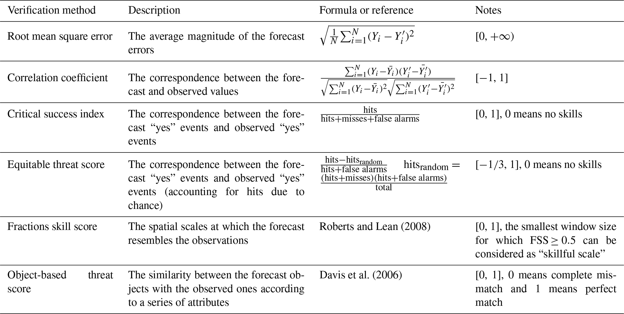

Table 1 Summary of the verification methods used in the paper.

To ease the comparison between the baseline models and the simplistic persistence forecast, we furthermore calculate skill scores (except for the FSS). In general, a skill score (SS) can be constructed by considering the target score S_m of the model, the score obtained with the reference forecast S_ref, and the perfect score S_perf:

$$\begin{array}{}\text{(6)}& \text{SS}={\displaystyle \frac{S_{\mathrm{m}}-S_{\mathrm{ref}}}{S_{\mathrm{perf}}-S_{\mathrm{ref}}}}.\end{array}$$

The higher the SS is, the better the model performs against the reference score. Perfect models thereby obtain SS=1, while inferior models show up with $-\mathrm{\infty }<\text{SS}<\mathrm{0}$. Note that S_perf=0 holds for the RMSE, whereas the other scores under consideration attain S_perf=1. Since the size of our dataset is not unlimited, we also apply a block bootstrapping procedure to estimate sampling uncertainty (Efron and Tibshirani, 1994). The block bootstrapping procedure accounts for autocorrelation between the sliding sequences and thus divides the dataset into non-overlapping blocks before the resampling of the blocks with replacement is performed. Here, we set the block length to 10 h (60 frames) and perform 1000 block bootstrapping steps.

4 Results

4.1 Quantitative evaluation

4.1.1 Point-wise evaluation metrics

In Fig. 3a–d, our model is compared to the baseline models in terms of the skill scores for the grid-point-level evaluation metrics (CC, RMSE, CSI, and ETS). The skill scores are calculated by defining the Eulerian persistence as reference forecast. It is seen that the deep learning models (i.e., ConvLSTM, PredRNN-v2 and CLGAN), as well as the optical flow model DenseRotation, outperform the persistence forecast after 20 min lead time in terms of the continuous scores (CC and RMSE). Among the video prediction models, PredRNN-v2 is superior over the others after the first 20 min, while ConvLSTM performs best for the longer lead times. CLGAN is not so competitive for RMSE and CC as PredRNN-v2 and ConvLSTM, while it still outperforms the traditional optical flow model DenseRotation. Note that the Eulerian persistence performs well in the first 10 min. One possible reason why these complex models can barely beat the persistence forecast in the first lead step is that the precipitation systems are relatively invariant within this very short time period. In our case, the Eulerian persistence forecast is the latest of the observations available, which is hence highly correlated to the ground truth at short lead times. With increasing lead times, its performance degrades quickly.

The comparisons in terms of the dichotomous scores (CSI and ETS) are given in Fig. 3c and d. They demonstrate that CLGAN is superior to the other competitors at all the lead times for simulating heavy precipitation events (the threshold t_Pr is set to 8 mm h⁻¹ here). The optical flow model DenseRotation performs well in the first 40 lead minutes, while its skill scores decrease rapidly afterwards. By contrast, the advanced deep learning model PredRNN-v2 shows more potential for longer lead times. Although ConvLSTM outperforms on the continuous scores, it can barely capture the heavy precipitation events. A large performance degradation for the ConvLSTM is diagnosed at a lead time of 20 min. One reason of the difference is that the model performance is evaluated with the skill scores, which are affected by the choice of the reference model (here the Eulerian persistence). For the first time step (lead time of 10 min), both ConvLSTM and Eulerian persistence can capture strong precipitation events, and ConvLSTM is even better. However, ConvLSTM models are prone to produce blurry predictions in an autoregressive prediction task, where the errors in the prior forecasts are inherited to the later ones. Hence, the ConvLSTM model gets less efficient in the next few lead steps, while the Eulerian persistence performs fairly well. For longer lead times, the performance of the Eulerian persistence forecasts quickly degrades, and ConvLSTM again outperforms the persistence model with positive skill scores.

The comparisons of the model performance show that CLGAN is superior in terms of scores for dichotomous forecasts (CSI and ETS), while it is less competitive in terms of RMSE. This is due to the fact that our CLGAN encourages the model to generate forecasts which have a similar distribution as the ground truth data rather than just reducing the averaged point-wise loss. Hence, more heavy precipitation events are predicted by the CLGAN model, which improves the dichotomous forecast scores. However, more predicted high-value precipitation could cause larger biases, compared to the models only generating low-value forecasts. The problem is magnified with the use of the point-by-point scores, i.e., the RMSE, which suffers from the double penalty issue.

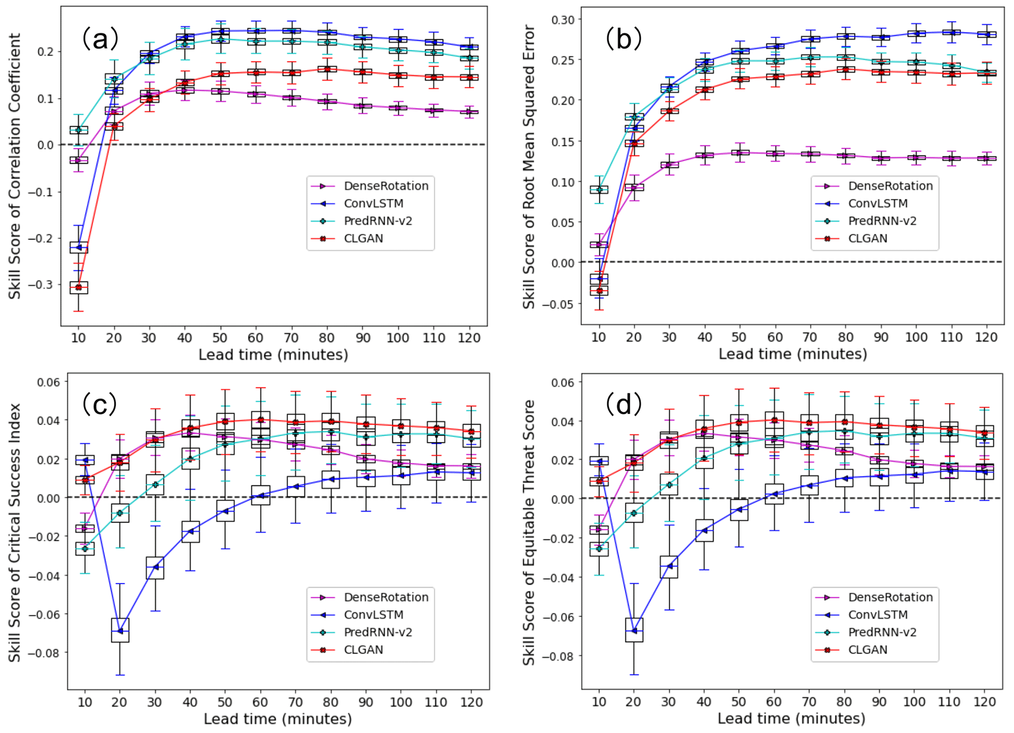
Figure 3 Box–whisker plots for skill scores of (a) CC, (b) RMSE, (c) CSI, and (d) ETS averaged over the testing period with the Eulerian persistence as the reference forecast. The boxes show the range of the first quartile (upper) to the third quartile (bottom) of the skill scores, and the whiskers denote the 95th percentile (upper) and 5th percentile (bottom), respectively. The threshold t_pr of CSI and ETS is 8 mm h⁻¹.

4.1.2 Spatial verification scores

To further investigate the model performances, we now turn our attention to the spatial verification scores, the FSS, and the MODE framework. Figure 4a shows the model performance in terms of the FSS for a lead time of 60 min by the persistence model (used as the reference forecast). The FSS is computed based on different neighborhood sizes and thresholds of hourly precipitation rates. Specifically, the neighborhood scale s in kilometers varies along the x axis. The FSS values for s attaining values of approximately 41, 69, 96, 152, and 290 km (square boxes of 3, 5, 7, 11, and 21 grid points, respectively) are plotted and marked as box–whisker plots for varying precipitation thresholds. The boxes show the range of the first quartile (upper) to the third quartile (bottom) of the scores, and the whiskers are, respectively, the 95th percentile (upper) and 5th percentile (bottom). As the threshold increases, FSS decreases, indicating that the persistence forecasts become increasingly imprecise for stronger precipitation events with a given spatial scale. For precipitation events exceeding t_Pr=8 mm h⁻¹, the persistence forecasts are considered useful (FSS≥0.5; see, e.g., Roberts, 2008) for a neighborhood scale of s≈69 km. Thus, the spatial accuracy of capturing these events is already fairly degraded, and the neighborhood scale of s≈69 km (five grid points) is applied to compute the FSS for other models in the following. Figure 4b compares the models' performance in terms of the FSS for heavy precipitation forecasting against the Eulerian persistence by illustrating the difference $\mathrm{\Delta }\text{FSS}={\text{FSS}}_i-{\mathrm{FSS}}_{\mathrm{ref}}$. Here, FSS_ref denotes the reference persistence model, whereas i is used to denote the other competing models. It is seen that all baseline models except from the ConvLSTM model can remarkably improve the spatial forecasting of such events, especially for longer lead times. Among them, CLGAN is superior to the others at all the lead times. DenseRotation performs well in the first lead hour, while PredRNN-v2 is promising for the further lead times.

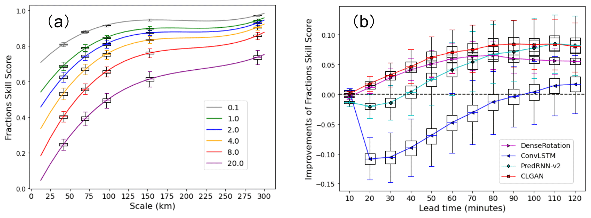
Figure 4 (a) FSS of persistence for different scales and intensity thresholds at 60 lead minutes for precipitation nowcasting. (b) Improvements in different models compared with persistence in terms of FSS with a threshold t_pr of 8 mm h⁻¹ and a neighborhood size of five. The boxes show the range of the first quartile (upper) to the third quartile (bottom) of the skill scores, and the whiskers denote the 95th percentile (upper) and 5th percentile (bottom), respectively.

4.1.3 Object-based diagnostic evaluation

To fully access the performance of the models in predicting spatial precipitation attributes, i.e., area, location, and shape, the MODE verification framework is applied. In the following, we present conditional quantile plots for the object area, for the location of the object centroid in east–west and north–south directions, for the aspect ratio, and for the orientation angle of the precipitation objects to show more details of predicted and observed precipitation objects. These plots visualize the joint distribution of the predictions and forecasts in a compact manner by applying a factorization into a conditional and marginal distribution (Murphy and Winkler, 1987; Wilks, 2011). Figure 5 illustrates the joint distribution in terms of the likelihood base-rate factorization. While the solid lines illustrate the forecasts conditioned on the observations for all models, the marginal distribution of the observations is plotted as a histogram. Figure 5a shows the number of grid points of the observed and predicted precipitation objects, which represents the area of precipitation objects. It can be seen that CLGAN and PredRNN-v2 are able to capture object area fairly well. Only objects consisting of 90 to 130 grid points (∼16 000 km²) are slightly underestimated (see Fig. 5a). However, the other competing models perform remarkably worse. Figure 5b and c show the distance between the centroid of the precipitation object and the western boundary and the southern boundary, which is again measured by the number of grid points. It is seen that the location of object centroids is generally well captured by all models. Stronger deviations are visible near the lateral boundaries, especially in the east–west direction. The aspect ratio and the orientation angle are used to assess the predicted precipitation shape in Fig. 5d and e. Here, the aspect ratio is the ratio of the shorter to the longer edge of the precipitation objects. The orientation angle constitutes the angle between the precipitation objects and positive x axis. CLGAN shows slight improvements over the other models in that the central parts of the orientation angle and aspect ratio are well calibrated. However, larger deviations from the 1:1 reference line are obtained near the tails of the conditional distributions. This indicates that further work on the simulation of precipitation shape is required.

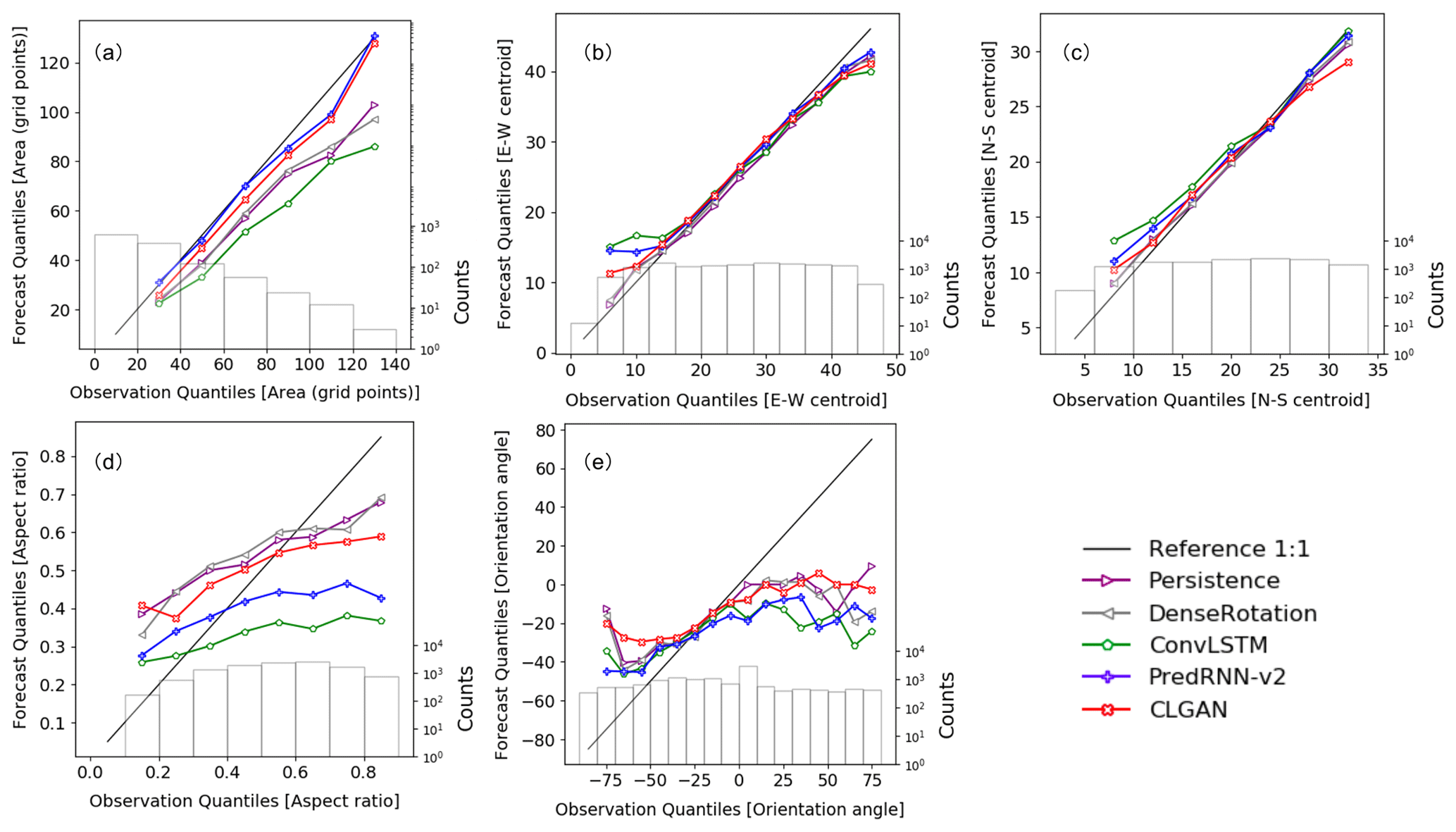
Figure 5 Conditional quantile plots in terms of the likelihood base-rate factorization for (a) area, (b) east–west centroid and (c) north–south centroid locations, (d) aspect ratio, and (e) orientation angle at the lead time of 60 min. The solid black line is the 1:1 reference line. The marginal distribution of the observations is presented as a histogram.

4.2 Case study

To gain further insight into the realism of our predictions, a heavy precipitation event occurring on 12 June 2019 is visualized as an example (see Fig. 6) to compare the model performance with an “eyeball” analysis. Figure 6a shows the observed precipitation rates in millimeters per 10 min for every 20 min over the forecast period starting at 06:50 CST. It is seen that a fairly strong precipitation system moves from west to east while it further intensifies. The predictions of the different models are presented as difference plots in Fig. 6b–f. For the first 60 min, persistence and DenseRotation show up with the smallest discrepancies. However, for longer lead times, clear dipole structures in the difference plots indicate that the movement of the system is not captured. Thus, the Lagrangian persistence framework is inaccurate for longer lead times, and more advanced models are required to capture the long-term dependence.

While the deep learning models also show increasing differences with longer lead times, they perform better in capturing the movement and the intensification of the precipitation system (see Fig. 6d–f). PredRNN-v2 tends to overestimate the precipitation intensity, which causes large coherent areas of positive differences. The averaged RMSE over the study area of the PredRNN-v2 forecasts at the lead time of 2 h is around 0.37 mm. ConvLSTM and CLGAN perform even better with smaller discrepancies, with a lower RMSE of 0.33 and 0.34 mm, respectively. Consistent with the quantitative evaluation results, ConvLSTM outperforms the CLGAN model in terms of RMSE in this given case, whereas CLGAN obtains a higher CSI and ETS. The CSI of the CLGAN forecasts with a threshold of 8 mm h⁻¹ at the 2 h lead time is around 0.11, 0.01 higher than the ConvLSTM model. The results demonstrate that the prediction by ConvLSTM has a lower bias, while CLGAN can capture more heavy precipitation grid points. Compared to ConvLSTM, the difference plot of CLGAN contains more fine structures which indicates that CLGAN can generate more details of the precipitation system.

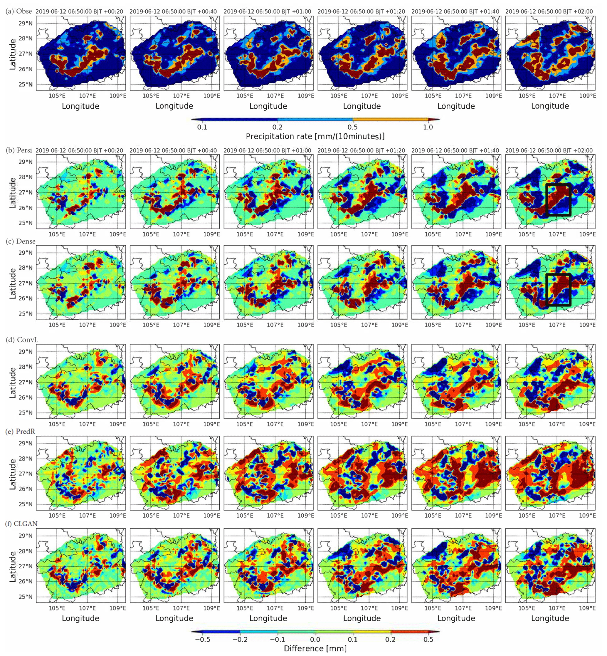
Figure 6 A case study for a rain system moving from west to east while intensifying. (a) Observation (Obse). The predictions of all models are illustrated with difference plots: (b) persistence (Persi), (c) DenseRotation (Dense), (d) ConvLSTM (ConvL), (e) PredRNN-v2 (PredR), and (f) CLGAN. The initial time of the prediction period is 06:50 CST on 12 June 2019.

4.3 Ablation study

As shown in Eq. (3), the loss function used in our CLGAN model consists of two terms: the adversarial loss ℒ^GAN and the reconstruction loss ℒ². To assess the contribution of each loss term on the forecasts' performance, sensitivity experiments on the weight of the reconstruction loss in CLGAN were carried out. Larger weight of the adversarial loss (equals smaller weight of reconstruction loss) is equivalent to a stronger contribution made by the GAN component. Figure 7 presents the results of the CLGAN model with different weights λ assigned to the ℒ² loss. It is seen that the RMSE is increased when reducing the weight of ℒ² loss (Fig. 7a). However, the scores for dichotomous events and fuzzy verification framework reveal improvements for smaller λ. The model using a pure reconstruction loss (λ=1 in Eq. 3) performs significantly worse than the model applying an adversarial loss in terms of CSI and FSS (Fig. 7b and c). Similar results are obtained in terms of the OTS (see Fig. 7d). The results of sensitivity experiments indicate that the adversarial training with the GAN component encourages the model to generate forecasts which are more similar to the ground truth data. Despite a slight increase in RMSE, a relatively stronger contribution of the GAN component helps to capture the statistical properties of the observed precipitation (on the tail, as well as their spatial attributes) which in turn improves the prediction of strong precipitation events.

Figure 7 Mean scores (a: RMSE; b: CSI; c: FSS; and d: OTS) for all lead times over the verification period for different weights of the ℒ² loss in CLGAN. The terms “weight1”, “weight999”, “weight99”, and “weight9” denote the weights of the ℒ² loss component λ with the corresponding values of 1, 0.999, 0.99, and 0.9, respectively. As in Fig. 3, t_Pr=8 mm h⁻¹ is chosen for CSI, OTS, and FSS, together with setting s to five grid points for the latter. The area threshold t_A of OTS is set to nine grid points.

5 Conclusion and discussion

A novel architecture CLGAN is proposed in this work which leverages the merits of U-Net, ConvLSTM, and GAN components to generate high-quality precipitation predictions up to 2 h over Guizhou, China. The Eulerian persistence is used as the reference model to compare against the conventional optical flow method DenseRotation, as well as two competing video prediction models (ConvLSTM and PredRNN-v2). A Guizhou AWS_ML precipitation dataset is set up for the nowcasting task based on minute-level precipitation measurements of AWS gauges. The model performance is comprehensively evaluated by a series of domain-specific evaluation metrics, including point-by-point and object-based verification methods. The results demonstrate that DL-based video prediction models are generally superior to the conventional methods, especially for the lead times exceeding 60 min. However, the use of grid-point-level losses (e.g., ℒ¹ or ℒ² loss) diminishes their capability to capture heavy precipitation events. Since heavy precipitation events are strongly under-represented in the data during training, the models optimized solely on grid-point-level losses favor predicting weak precipitation rates to avoid large error contributions from strong precipitation events (double penalty problem). By contrast, the GAN component of CLGAN encourages the generator to create predictions that share the statistical properties of observed precipitation, which makes it superior to the baseline and the competing models in dichotomous and spatial scores for heavy precipitation events.

Compared to the conventional methods, our results indicate that video prediction models with deep neural networks have a better capability of learning abstractions from data, which in turn can improve the prediction of complex evolving systems. By learning the statistical dependency within the continuous sequence of precipitation data, video prediction models can simulate the precipitation patterns up to 2 h ahead fairly well. Since NWP models suffer from the spin-up issue in the first 6 h and the conventional approaches fail to capture long-term dependency, video prediction models show potential as a promising and reliable way for precipitation nowcasting. However, a model performance degradation is expected for longer lead time, i.e., after 2 h, due to the error accumulation in the auto-regressive prediction task. The quick evolution of the convective precipitation systems is furthermore challenging. Our results also demonstrate that it is arduous to capture the shape of precipitation patterns by DL-based models as demonstrated by the MODE scores. Future work may try to integrate domain-specific evaluation metrics for spatial forecasts (e.g., FSS and MODE) as a loss function in DL-based models for precipitation nowcasting. Additionally, we also see that a trade-off exists between evaluations on grid-point and object-based levels when the adversarial loss is varied. A grid search for the optimal combination of loss function coefficients is required to generate realistic forecasts with a low bias.

Beyond that, it is appealing to embed more predictors which could be retrieved from NWP models, e.g., the vertical velocity, water vapor, and thermal and other environmental conditions. The literature shows that the corresponding predictors and physical constraints can greatly improve the simulation of the targeted variable (Daw et al., 2017; Gong et al., 2022). A careful selection of the predictors and an appropriate embedding solution are subject to our future work. In addition, GAN models can easily be adapted to a probabilistic framework. By adding noise as an additional input, ensemble forecasts can be obtained from which a quantification of the forecast uncertainty can be deduced (Mordido et al., 2018). A probabilistic nowcasting system is appealing due to the strong inherent uncertainties in the dynamics of precipitation patterns. Furthermore, note that ensemble predictions corresponding to several future realizations provide the possibility to issue more strong precipitation events (cf. Ravuri et al., 2021). While this study focused on assessing the need for an adversarial loss formulation, future work will be directed towards a probabilistic nowcasting system.