the Creative Commons Attribution 4.0 License.
the Creative Commons Attribution 4.0 License.
 | 11 May 2023
Global seamless tidal simulation using a 3D unstructured-grid model (SCHISM v5.10.0)
Y. Joseph Zhang
Tomas Fernandez-Montblanc
William Pringle
Hao-Cheng Yu
Linlin Cui
Saeed Moghimi
We present a new 3D unstructured-grid global ocean model to study both tidal and nontidal processes, with a focus on the total water elevation. Unlike existing global ocean models, the new model resolves estuaries and rivers down to ∼8 m without the need for grid nesting. The model is validated with both satellite and in situ observations for elevation, temperature, and salinity. Tidal elevation solutions have a mean complex root-mean-square error (RMSE) of 4.2 cm for M2 and 5.4 cm for all five major constituents in the deep ocean. The RMSEs for the other four constituents, S2, N2, K1, and O1, are, respectively, 2.05, 0.93, 2.08, and 1.34 cm). The nontidal residual assessed by a tide gauge dataset (GESLA) has a mean RMSE of 7 cm. For the first time ever, we demonstrate the potential for seamless simulation on a single mesh from the global ocean into several estuaries along the US West Coast. The model is able to accurately capture the total elevation, even at some upstream stations. The model can therefore potentially serve as the backbone of a global tide surge and compound flooding forecasting framework.
- Article
(11952 KB) - Full-text XML
- BibTeX
- EndNote


Global ocean modeling traditionally focuses on large-scale processes but is increasingly looking into the roles played by smaller-scale processes (internal gravity waves (IGWs), topographic waves, lee waves, etc.) in the global energy budget (see a review done in Arbic et al., 2018, hereafter A18). The state-of-the-art global ocean models now boast or finer resolution (thus fully eddy resolving) (A18). More and more models are incorporating barotropic and/or baroclinic tides in their simulation due to their importance in ocean mixing and global energy budget. Table 1 summarizes the major characteristics of several global tide models. Both structured-grid-based and unstructured-grid-based models have been successfully developed for global tides, starting from the simpler 2D barotropic model, with or without assimilation of altimetry observation. Prominent examples include the highly accurate altimetry-informed TPXOv9 (Egbert and Erofeeva, 2002) and FES2014 (Lyard et al., 2021) tidal databases. Recently, Pringle et al. (2021) used a 2D model to accurately simulate tide and surge concurrently with high-resolution areas of the mesh focused on hurricane landfall regions. While such a 2D model cannot simulate baroclinic effects, it has been suggested that including a baroclinic term derived from a separate 3D ocean circulation model could be used to improve the energy spectrum of modeled sea surface heights, particularly at the low-frequency end (Pringle et al., 2019). The 3D baroclinic models that include concurrent simulation of eddying circulation and tidal motion are also becoming feasible (Arbic et al., 2010; Savage et al., 2017). Wang et al. (2022) recently proposed a reduced-layer (nine layers) 3D baroclinic model with nudged temperature and salinity fields for improving operational total water level forecasts.
As the global ocean constitutes a quasi-closed system, simulating global ocean processes with both tidal and nontidal frequencies should include coastal oceans, where most of the tidal energy is dissipated; collectively, the shelves dissipate about 70 %–75 % of the tidal energy (A18). Also, as A18 mentioned, improving nearshore tides will have a back effect that will also improve open-ocean tides, especially in tidally energetic areas (e.g., the North Atlantic). Accurately accounting for this dissipation process requires high-resolution nearshore data to represent the complex geometry and bathymetry found therein, which represents one of the grand challenges in ocean modeling (Holt et al., 2017). In fact, we suspect that the need for several additional types of drags (wave drags, etc.) in the global ocean modeling in contrast to basin-scale modeling might be related to the inadequate representation of coastal oceans, as even the state-of-the-art resolution of (Savage et al., 2017) is hardly resolving the coastal features. The need for high resolution in the coastal ocean would inevitably strain the already high computational cost associated with global simulations, and in this regard unstructured-grid (UG) models can effectively mitigate the cost. To this day, however, few UG global models resolve both tidal and nontidal processes. Logemann et al. (2021) assessed the impact of coastal refinement on tides using an UG global ocean model but did not systematically compare their results with the TPXO solution in the deeper ocean, and the reported error metrics appear unsatisfactory.
Despite the tremendous progress made, so far no 3D models for the global ocean exist that can simultaneously include estuaries and rivers without resorting to grid nesting. This is related to the very different characteristics between global and coastal oceans and estuaries (Fringer et al., 2019); chief among those differences are the drastically different spatial scales and force balances (e.g., geostrophic vs. ageostrophic, weakly forced vs. strongly forced regimes). The stability and efficiency constraints that come with resolving small-scale processes as commonly found in the coastal and estuarine regimes are formidable. For this reason, some global models have or are developing their own versions of “coastal model” components that are intended to be nested into the corresponding global models to better close the energy budget (e.g., Andosov et al., 2019).
In this paper, we present a new 3D baroclinic UG model for the global ocean that incorporates both tidal and nontidal processes and their interactions and is capable of resolving both ocean basins and estuaries with a single mesh. For topics as large as this, inevitably we have to focus on a subset of interests. Here we focus on the short-term predictability (on the scale of 1 year or shorter) of the total water level (TWL) including both tidal and nontidal components for both large and small scales simultaneously, with the ultimate goal of building a global storm tide and compound flood operational model that resolves both eddying motions and some small-scale processes found near the islands and inside estuaries and rivers of interest. This represents a bold approach of ocean modeling that would completely do away with the need for open boundary conditions as in the case of regional models and can also effectively close the last remaining gap in the energy budget in the global ocean.
We will first describe in Sect. 2 the observational datasets used in this paper, as well as the 3D UG model and its setup for the global ocean simulation. We proceed to model validation and assessment of tidal and nontidal elevation, temperature, and salinity in Sect. 3. In Sect. 4, we highlight the importance of representation of the ice shelves near Antarctica in the model bathymetry and feedback from shallow areas. Lastly, we demonstrate the model's potential capability of capturing small-scale processes inside estuaries with the focus on TWL prediction in the shallows (including the challenging upstream area); more detailed quantitative assessment for 3D processes would entail site specific calibration and is left for future study. We also discuss the need for closing the gaps in the theoretical understanding of the cross-scale processes. A short summary is presented in Sect. 5.

2.1 Observation
In this paper we will primarily validate the model using a satellite-derived reanalysis product OSTIA (for sea surface temperature, SST, https://data.marine.copernicus.eu/product/SST_GLO_SST_L4_NRT_OBSERVATIONS_010_001/description; last access: May 2023), an altimetry-informed global tidal model TPXOv9, a global tide gauge dataset (GESLA; Woodworth et al., 2016a) for sea surface height (SSH), and ARGO floats (Wong et al., 2020) for temperature and salinity profiles. Tide gauge observations will be used sparingly as most of these are located in complex nearshore regions that require accurate bathymetry information and more mesh work to capture that information. We will use a few tide gauge data for a target study of the US West Coast in Sect. 4. Our ultimate goal is to build a global 3D UG model that is able to seamlessly transition from ocean basin into small creeks; to achieve this goal, however, it is essential to first ensure that the model has sufficient skill for large-scale processes. We note that the current 3D UG model has been extensively applied and validated in many coastal regions, meaning that the latter does not present fundamental challenges for the model as long as a proper calibration procedure is followed.
2.2 Model description
SCHISM (schism.wiki) is an open-source community model solving the 3D hydrostatic form of the Navier–Stokes equation with Boussinesq approximation (Zhang et al., 2016). Major innovative features of SCHISM include (1) a semi-implicit time-stepping scheme that bypasses the most stringent stability constraints (and thus allows very fine resolution of O(1 m) without the need to reduce the time step); (2) a highly flexible 3D gridding system, with a hybrid quadrangular–triangular unstructured mesh in the horizontal dimension and localized sigma coordinates with shaved cells (LSC2) in the vertical dimension (Zhang et al., 2015), where the flexible gridding system enables powerful “polymorphism”, with a single SCHISM grid being able to seamlessly morph between full 3D, 2D depth averaged (2DH), 2D laterally averaged (2DV), and quasi-1D configurations (Zhang et al., 2016); and (3) a judicious combination of higher- and lower-order schemes to ensure accurate representation of diversity of processes from creek to ocean basin scales (Zhang et al., 2016; Ye et al., 2019). These features have previously allowed a single model to be used for challenging compound flooding studies that involve coastal transition zones between hydrodynamic and hydrologic regimes forced by ocean, atmosphere, and watershed rivers (Ye et al., 2020, 2021; Zhang et al., 2020; Huang et al., 2021). Global compound flooding processes are not the focus of this paper.
The global unstructured mesh in the horizontal dimension consists of ∼4.6 million nodes and ∼9 million triangular elements with a nominal resolution of 10–15 km in the ocean basin (Figs. 1–2), and it is thus barely eddy resolving. The mesh resolution generally increases to ∼3 km at most of the coastline of the continents or islands; a higher resolution of ∼1–2 km is applied in North America and the western Pacific due to our interests in those regions. As an illustration, we have also added detailed representations of a few estuaries and rivers along the US West Coast (Fig. 1b–e). In Sect. 4.3 we demonstrate the model's potential for seamless cross-scale transition into nearshore areas and estuaries, with a minimum element size of ∼8 m found near a coastal highway inside the Columbia River estuary (Fig. 1e). Therefore, the mesh size spans 4 orders of contrast (from ∼10 km to ∼8 m). Overall, about 50 % of the elements have a resolution of 5 km or higher (Fig. 2c).
Consistent with our main goal in this paper, we use GEBCO (GEBCO Compilation Group, 2019) as the main DEM source, with a resolution of 500 m for global oceans. This resolution is adequate in most of the coastal and deep oceans but is not sufficient for nearshore areas and estuaries. As shown in Sect. 4.1, it is important to include the ice shelf effect on the bathymetry in the Southern Ocean, and we therefore use RTOPO for this purpose (Schaffer et al., 2016). To improve the model skill in the target estuaries on the US West Coast, we have locally utilized a hierarchy of DEMs from NOAA's Coastal Relief Model (∼90 m resolution), CUDEM (1–10 m resolution; CUDEM, 2022), and USGS's CoNED (1–3 m resolution; CoNED, 2022).
The 3D model takes full advantage of the flexible vertical gridding system (LSC2; Zhang et al., 2015). The number of sigma layers varies from a maximum of 34 to 1 (i.e., 2DH configuration) at mesh nodes, and the average number of layers among all nodes is 32. Using 1 layer in shallow and dry areas (where the first master grid depth is less than 0.4 m; cf. Zhang et al., 2015) greatly improved the efficiency and robustness of the model (Huang et al., 2021). The second master grid depth is set at 10 m with 23 layers in order to have adequate resolution for the vertical stratification in shallows (cf. Zhang et al., 2015). The vertical high resolution is focused on the near-surface zone at the expense of the bottom in order to conserve computational cost. As a result, the near-bottom vertical layers can be as thick as 1 km in the deep ocean; in other words, the logarithmic bottom boundary layer at deep depths is not well resolved, and we therefore apply zero friction in the deep depths. To ensure adequate energy dissipation toward shallows, we use a simple depth-dependent bottom friction coefficient (used in the quadratic drag formulation) that linearly increases from 0 at a depth of 200 m to 0.0025 at 50 m:
where h is the local depth and h1=50 and h2=200 m are the two transition depths with corresponding friction coefficients of Cd1=0.0025 and Cd2=0, respectively. We have also tried Cd2=0.0001, and the results are similar. For the sake of simplicity, no attempt has been made to optimize the friction in each region yet, and this is left for future work.
A main advantage of using a 3D baroclinic model is that it accounts for internal tides (ITs), whose production over open-ocean topographic features accounts for about 25 %–30 % of the energy lost in the global barotropic tidal energy budget (A18). The results from Egbert and Ray (2003) suggest IT dissipation is an important contributor to the mixing that underpins the large-scale circulation (Munk and Wunsch, 1998). According to A18, a horizontal resolution of at least is needed for a fully vigorous low-mode IT field. On the other hand, a horizontal resolution of about or finer is necessary for simulating a vigorous IGW continuum. Therefore, the current model, because of the limited computational resources available to us, only resolves ITs but not IGWs. Although parameterized IGW drag formulation (e.g., Garner, 2005) could be included in the model, its inclusion in a baroclinic model is tricky as part of the signal is already resolved (A18). Therefore, we neglect IGW drag here.
The semi-implicit model uses a non-split time step of 120 s, a turbulence closure scheme of k-kl of the generic length scale model (Umlauf and Burchard, 2003) and a bi-harmonic viscosity (Zhang et al., 2016). Since no bathymetry smoothing was done in our mesh, the presence of very steep bottom slopes near numerous islands and ocean trenches requires additional momentum stabilization than provided by the bi-harmonic viscosity. Therefore, we add a Smagorinsky-type viscosity that is designed to “penalize” the steep slopes. In line with the Shapiro-filter-like implementation of viscosity inside SCHISM that works well with highly distorted UGs (Zhang et al., 2016), the Smagorinsky-type viscosity is implemented as follows:
where γ is the filter strength with a maximum value of 0.5 (Zhang et al., 2016), Δt is the time step, Γ is the deformation rate, and C is a non-dimensional constant specified by the user. In the global model, we found that C=1000 is sufficient to suppress most spurious noise in the horizontal velocity field. For tracer transport, the third-order WENO scheme (Ye et al., 2019) is used at depths greater than 10 m (whereas an upwind scheme is used for shallower depths).
Besides the Smagorinsky-type viscosity scheme, other new features of SCHISM developed in this work include (1) a self-attracting and loading (SAL) tides scheme, using the depth-dependent parameterization of Stepanov and Hughes (2004), and (2) an efficient asynchronous I/O using dedicated “scribe” cores, which is essential for large core counts and significantly improves parallel I/O and scaling. A continuously updated online manual that explains all SCHISM features can be found at http://www.schism.wiki (last access: 2 May 2023) or through Zhang et al. (2022).
The primary validation period used in this paper is a 120 d window from 1 June to 29 September 2011. Atmospheric forcing from ERA5 (with a resolution of 25 km) was applied onto the ocean surface, including wind, air pressure, precipitation, and heat fluxes. Relaxation of temperature and salinity near the ocean surface toward their climatologic values, which is commonly utilized in many global ocean models to prevent long-term drift in decadal- and century-scale simulations (Ringler et al., 2013), was not applied here due to the relatively short duration of the simulation. The tidal potential with five constituents (M2, S2, N2, K1, O1) and self-attracting and loading (SAL) tides were included. For the harmonic analysis and comparison with TPXOv9, we used the model results from days 20 to 60 and turned off the atmospheric forcing, as the 40 d results used were long enough to distinguish the five constituents used in the analysis.
The model was initialized with a dynamic flow field interpolated from the global (∼10 km) HYCOM. Linear interpolation was used in the interpolation of sea surface height (SSH), horizontal velocity, salinity, and temperature. Constant extrapolation was used in regions not covered by HYCOM. The HYCOM-derived SSH and horizontal velocity represent the nontidal component; once started, the tidal potential and SAL will initiate the tidal motion in the system. The 868 largest rivers were included along the coast with monthly mean flow information from Dai (2021). The river temperature input was set to be the “ambient” flow temperature due to the lack of such information. Starting the simulation from a fully dynamically equilibrated flow field allows us to significantly reduce the time required for warming up the model. Still, the discrepancies between HYCOM and SCHISM and initiation of the tides require a short ramp-up period, estimated to be shorter than 20 d.
We remark here on a few limitations of the current model. The need for IGW drag may be reassessed in the future. Alternative implementations of SAL, e.g., interpolation from TPXO or FES, should be explored. At high latitudes, the lack of an ice model is a major gap for the model; even though we have this component inside the SCHISM system, its inclusion would significantly increase the computational cost, especially under high mesh resolution. The mesh resolution in the deep ocean is barely eddy resolving; for accurate simulation of the eddying processes, finer mesh resolution would be required. Lastly, atmospheric forcing could use higher spatial and temporal resolution for a more accurate simulation of coastal processes, especially during storm events.
SCHISM's good parallel scaling allows efficient simulation given adequate resources. For example, on 5600 cores of an Intel cluster (TACC's Frontera) the model is able to run ∼120 times faster than real time. Doubling the core count to 11 200 increases this real-time ratio to ∼223, which translates to an excellent parallel efficiency of ∼95 %.
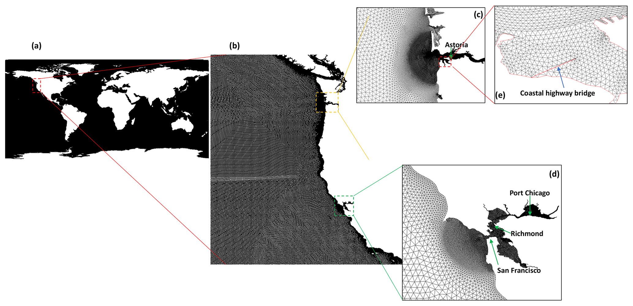
Figure 1(a) Global unstructured mesh, with (b) successive local refinements in the US West Coast, including (c, e) the Columbia River estuary and (d) San Francisco Bay.
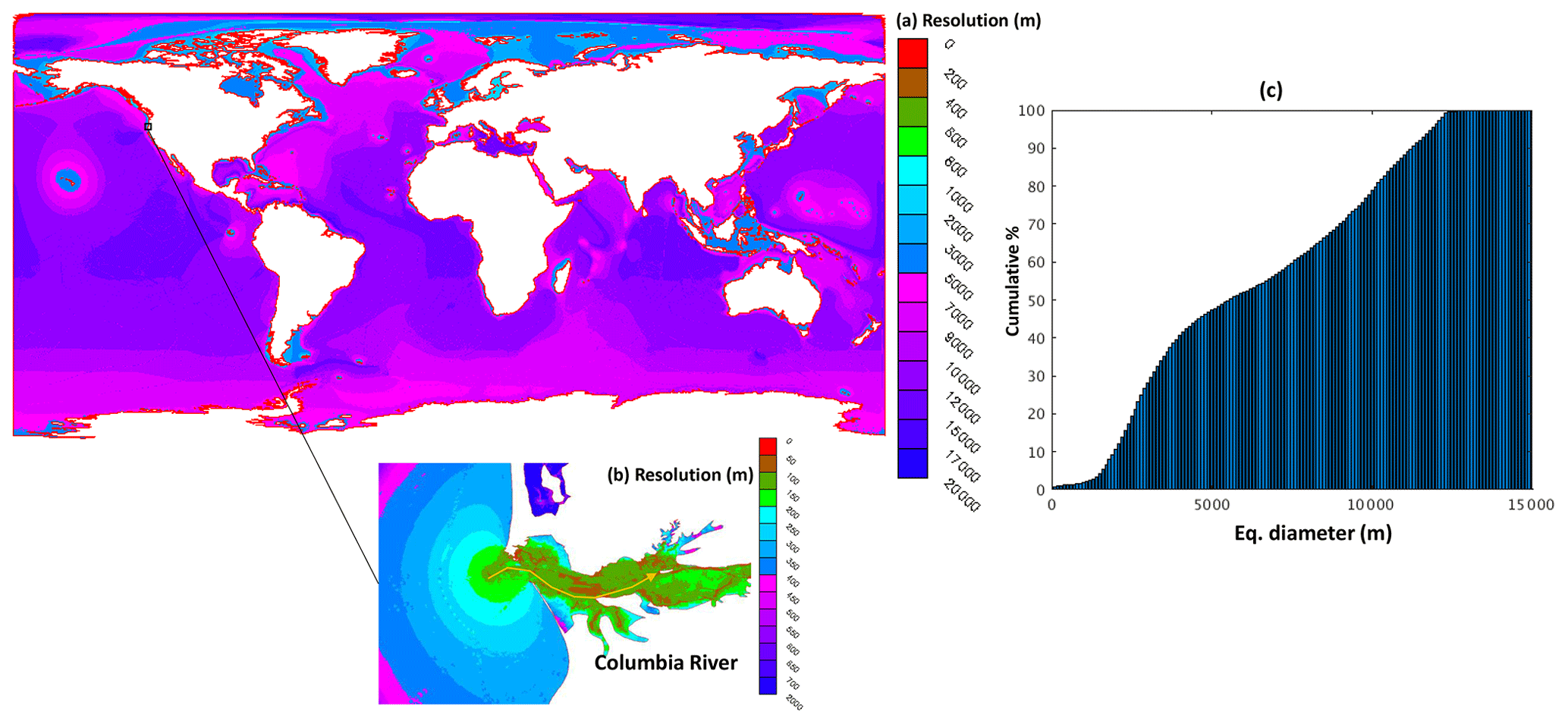
Figure 2(a) Mesh resolution as measured by equivalent diameter, with (b) a zoom-in near the Columbia River; the orange transect is used to show the salt intrusion path. (c) Histogram of resolution.
We start the model validation with surface elevation with respect to both tidal (Sect. 3.1) and nontidal components (Sect. 3.2). For 3D variables, we focus on temperature and salinity as these are the major drivers of the large-scale processes due to their contributions to the uneven oceanic mass distribution. Note that the focus of this study is on the accurate prediction of the total elevation. We follow HYCOM in using NGVD29 (geopotential) as the vertical datum, which is problematic in the assessment of either the altimetry (which is referred to a fixed geoid; Jahanmard et al., 2021) or some tide gauges that refer to different datums (e.g., NAVD88). More rigorous assessment of the total water level is left out for future studies after a geoid-based datum becomes available, and here we focus on the tidal elevation as well as the variability of the nontidal elevation (i.e., the mean biases are removed when data do not match or are unknown). Standard error metrics are reported below, including RMSE (root-mean-square error), MAE (mean absolute error), correlation coefficient, and Wilmot score (Willmott, 1981).
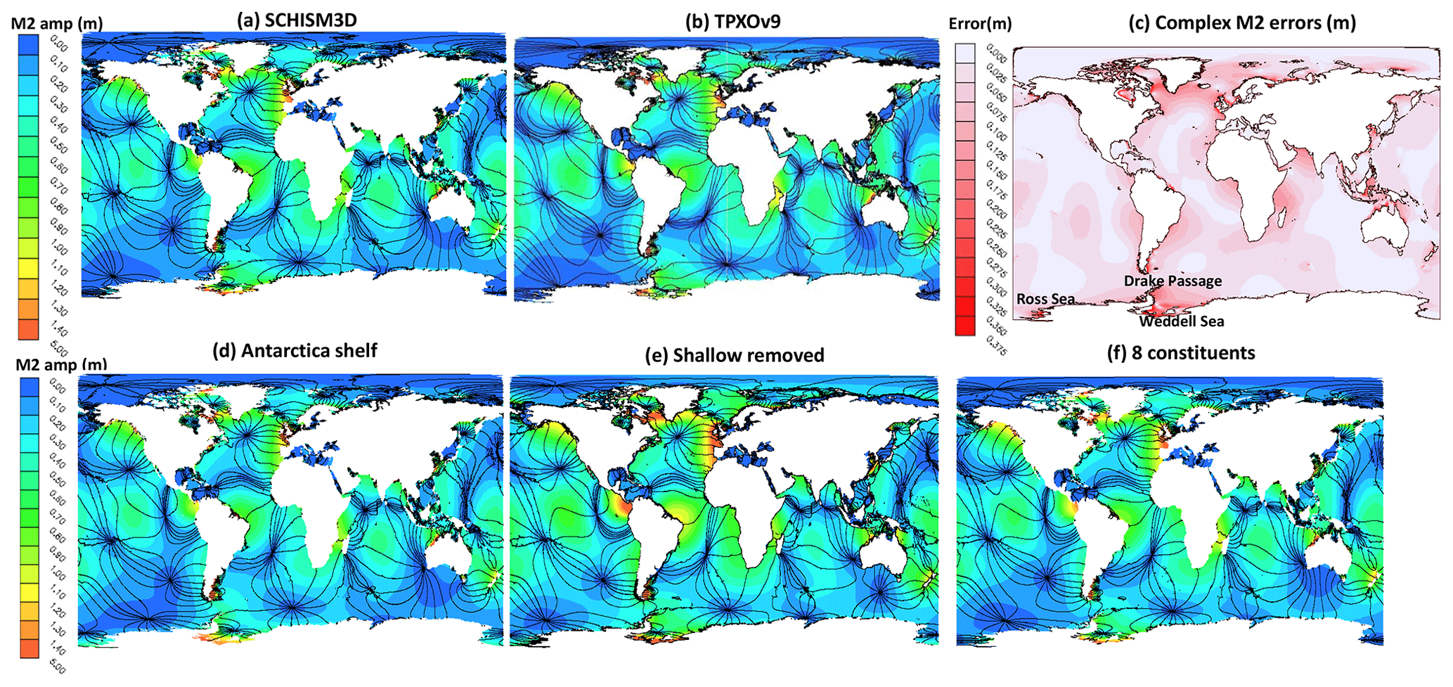
Figure 3Comparison of co-tidal chart for M2 between (a) SCHISM and (b) TPXOv9. The complex M2 RMSE is shown in (c); some geographic locations are labeled also here. (d) Sensitivity results without the Antarctic ice shelf represented. (e) Sensitivity results with shallow areas (<50 m) removed. (f) Sensitivity results using eight constituents.
3.1 Co-tidal chart for M2
Globally, the M2 amphidromes correspond to the local minimum of the tidal energy in the open ocean or near islands (e.g., Taiwan, New Zealand, Madagascar etc) where the tides tend to rotate in the form of Kelvin waves (Fig. 3b). The amplitude maxima, on the other hand, are typically found near semi-enclosed basins near resonant modes (e.g., European Seas, Hudson Bay, Bay of Fundy), where the tidal transformation is rather complex (Fig. 3b).
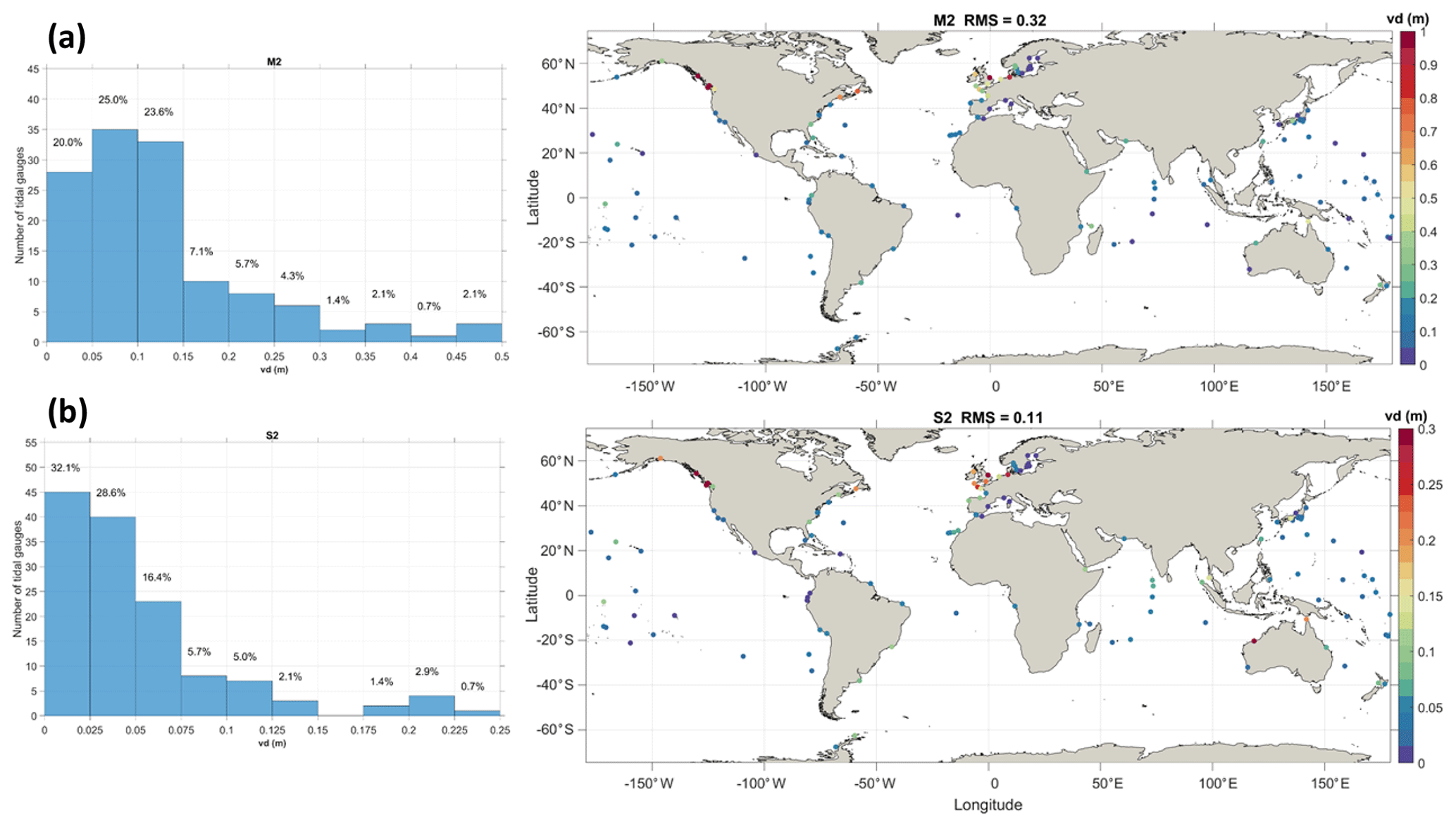
Figure 4Histogram and maps of scatterplots of M2 and S2 vector difference error.
A major benefit of the 3D model is that the time-varying dissipation of tidal energy due to internal tides is accounted for inside the model. Therefore, with a simple specification of bottom friction (as a function of depths), the simulated M2 distribution already has a good skill compared to the benchmark TPOXv9 tidal database (Fig. 3).
The complex RMSE for a constituent is defined as follows (Wang et al., 2012):
where VD stands for vector difference, A is the amplitude, “m” and “o” refer to model and observation, φ is the phase, and j is the constituent index. The area-averaged RMSE for a specific area Ω is then defined as follows:
The can be computed for a single constituent (e.g., M2) or summed up for a group of constituents (e.g., all five constituents) to give a single number for those constituents.
The averaged complex RMSE for M2 is 4.2 cm for depths greater than 1 km and 14.3 cm for shallower depths. The averaged total RMSE for all constituents is 5.4 cm (16.6 cm) for depths greater than (less than) 1 km. The breakdown of RMSEs for the other four constituents of S2, N2, K1, and O1 is 2.05, 0.93, 2.08, and 1.34 cm, respectively, for depths greater than 1 km and 6.07, 2.60, 4.71, and 2.84 cm, respectively, for depths shallower than 1 km. These results are slightly better than the previous best 3D model results without data assimilation (Schindelegger et al., 2018) but slightly worse than those in Pringle et al. (2021); for example, the total RMSE from their model is 3.9 cm (17.2 cm) in the deep (shallow) ocean. Note that there are differences in the shallow areas included in each model, which makes the numbers for the shallows less reliable than those for the deeper depths. In addition, the sensitivity results using eight tidal constituents (M2, S2, N2, K2, K1, O1, P1, Q1) are similar (Fig. 3f); the averaged complex RMSE for M2 is essentially the same as using the five constituents.
Our elevation results are quite satisfactory given the fact that minimal calibration (e.g., with respect to bottom friction) was conducted; the more complete physics as incorporated in the 3D baroclinic model reduced the amount of calibration required to achieve good tidal results compared to 2D barotropic models (e.g., Blakely et al., 2022). Our own experience with global SCHISM 2D and with regional studies (Huang et al., 2021, 2022; Ye et al., 2020) also confirmed that an elaborate calibration exercise using spatially variable friction was necessary to improve the elevation skill in the 2D model. Compared to other global 3D models, our model seems to be able to obtain satisfactory results without the need for some elaborate drag formulations described in A18; one plausible reason is that the higher resolution used in the coastal ocean has provided adequate energy dissipation with improved seafloor representation in areas with complex bathymetry and geometry.
3.2 GESLA tide gauges comparison
The modeled sea levels are compared with observed sea levels from tide gauge stations in the Global Extreme Sea Level Analysis (GESLA) dataset (Woodworth et al., 2016a). The tidal harmonic analysis is performed using the t-tide package (Pawlowicz et al., 2002). The skills of the model to reproduce tides are assessed using the RMSE for each tidal constituent (cf. Eq. 3), averaged over all tide gauges. Then the root sum of square (RSS) is used as an overall skill index:
where n=5 is the total number of constituents. The tidal skill scores are also computed from the FES2012 model, an altimetry-informed model used as a reference to evaluate our model.
The assessment of model performance to reproduce the nontidal residual (NTR) sea level variation is also conducted. Due to the uncertainty in the vertical datums used in many gauges, NTR time series are obtained by de-meaning for the common period and de-tiding using the t-tide package. Afterwards skill scores of RMSE and Pearson correlation coefficient are computed. In order to assess the model predictive skill for extreme water levels, RMSE and correlation scores are also computed for the upper tail of the time series, i.e., values exceeding 95th percentile of the observed NTR.
Overall, a satisfactory model performance is observed in coastal areas in comparison with GESLA. The model RMSEs are less than 0.1 m at ∼45 % of tidal stations for M2 and less than 0.05 m at ∼58 % of the stations for S2 (Fig. 4). The comparison with FES2012 indicates larger error in SCHISM (+6 cm in M2 RMSE and +2 cm for S2 RMSE) (Table 2). It is an acceptable performance given the fact that FES2012 incorporates data assimilation from altimetry data (Carrère et al., 2013). Most of the larger errors occur in areas with DEMs of large uncertainty (e.g., Canadian coasts with fjords, southern Chilean/Argentine coasts) or in areas with insufficient resolution (e.g., European seas) (Fig. 4). Consequently, the model comparison with GESLA produced larger errors than with the TPXOv9. The uneven error distribution may guide future priority in mesh development.
The model also accurately reproduces the NTR in coastal waters (Fig. 5). The average RMSE is only 7 cm with a median value of 6 cm; ∼88 % of RMSEs are below 10 cm and only 1.6 % exceed 15 cm, mostly at stations located in the North Sea and northwestern Pacific Ocean. The RMSE increases for extreme conditions (NTR > 95th percentile), but the model still adequately reproduces the extreme conditions with an averaged RMSE of 11 cm and a median of 9 cm. In addition, RMSEs are less than 15 cm at ∼80 % of the tidal stations under extreme conditions. These results are consistent with our previous results using the 3D model (Ye et al., 2020; Huang et al., 2021, 2022), and the better skill at capturing the NTR is indeed a major advantage of 3D over 2D models because the NTR is largely driven by the eddying motions and large-scale ocean current systems that originate from the uneven ocean mass distribution.
Table 2Summary of model performance to reproduce the main semidiurnal tidal component for SCHISM and FES2012 models against GESLA. The RMSE and RSS are averaged over all tide gauges.
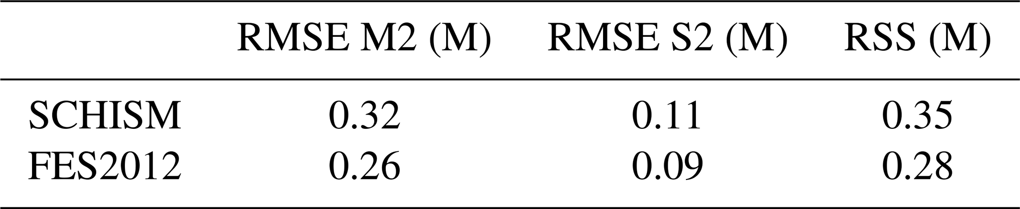

Figure 5Map and histogram of RMSEs for the nontidal residual (NTR); ∼88 % of RMSEs are below 0.1 m.
3.3 SST
The quality of the simulated sea surface temperature (SST) is assessed against a reanalysis product, OSTIA (Good et al., 2020), which blends different satellites with in situ data into regular 0.05∘ resolution sea surface temperature estimation on a daily basis. This dataset provides global SST with an overall analysis error of ∼0.4 ∘C. Most large errors are distributed in the Arctic region, which can reach 3.6 ∘C maximum. In order to isolate the effects from the Arctic, the analysis is done for the global domain with and without the Arctic region (latitude >60∘ N). The OSTIA analysis error excluding the Arctic is reduced to 0.3 ∘C on average.
The simulated SST is mostly similar to OSTIA (Fig. 6). In particular, the model is able to capture major boundary currents (Kuroshio, Gulf Stream, etc.) and equatorial instabilities. A closer look at the comparison reveals larger warm biases in the Arctic region (Fig. 7), which is not surprising because we did not include the ice component in our model. Excluding the Arctic, the averaged MAE stays much lower at ∼0.8 ∘C throughout the simulation period (Fig. 7b). Besides the high-latitude regions in the Northern Hemisphere, relatively high biases are also found near the boundary currents and equatorial instability regions (Fig. 7a).

Figure 6Comparison of SST between (a) OSTIA and (b) SCHISM at the end of the 120 d simulation (29 September 2011).
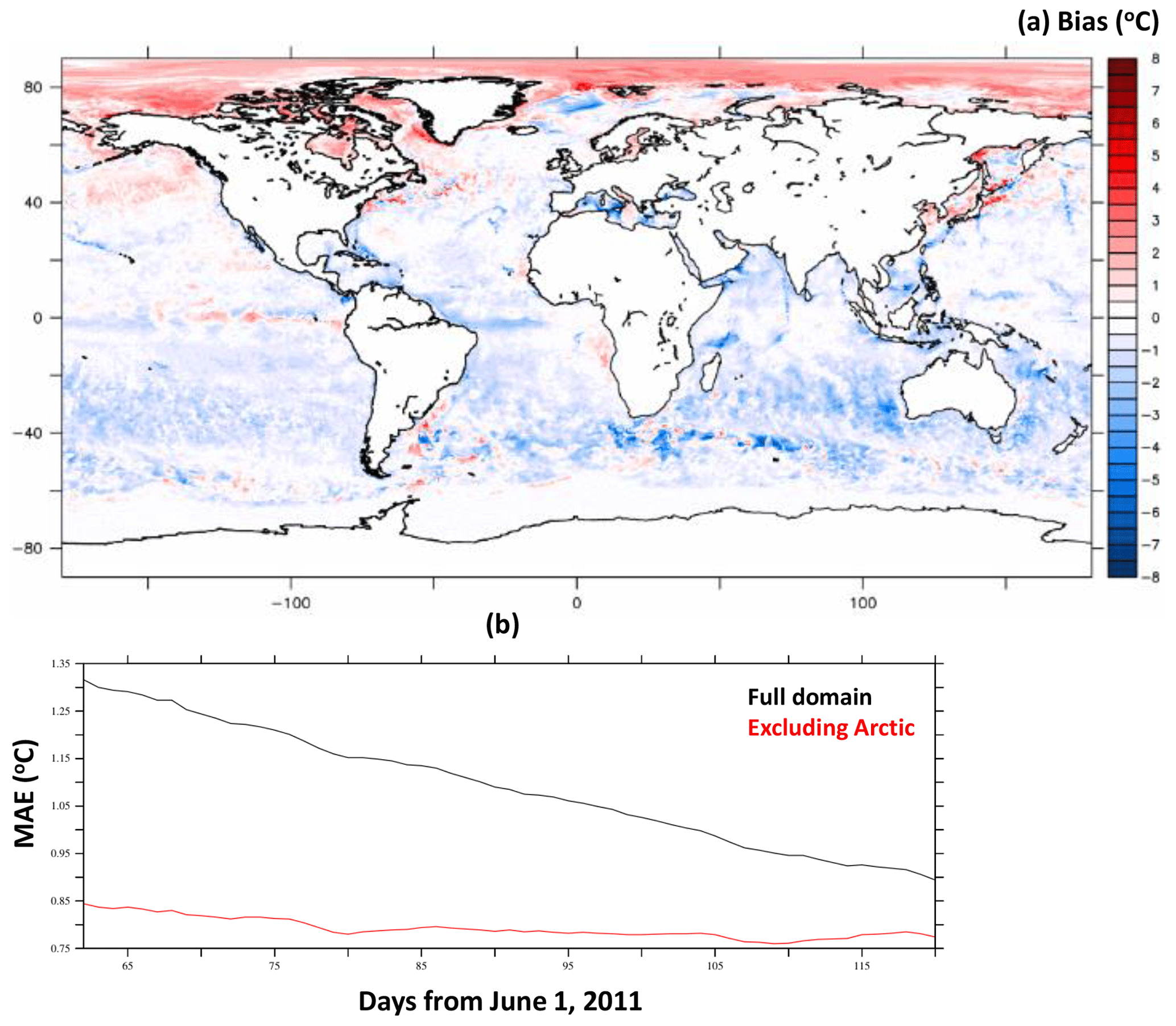
Figure 7SST from the 120 d run from 1 June 2011: (a) SST bias and (b) MAE.
3.4 SSS
Compared to SST observations, sea surface salinity (SSS) observations are scarcer. Although NASA's Aquarius satellite missions did cover the simulation period, the data may be too coarse for our purpose. Therefore, we use HYCOM (which has assimilated profile data) as a reference solution in our comparison. The two models are largely comparable, including major fronts and instabilities near the Equator, the freshwater plumes, and boundary currents, and intrusion from the North Atlantic into the Arctic (Fig. 8). Freshwater plumes from Amazon and other large rivers appear to be larger in SCHISM. Due to the absence of an ice component in our model, there are also some differences in the Arctic Ocean. Overall, the modeled SSS is satisfactory.
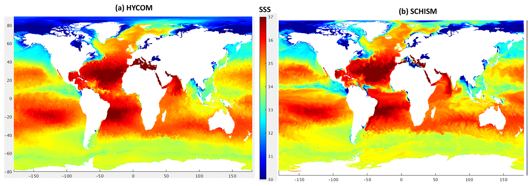
Figure 8Comparison of SSS between (a) 1/12∘ HYCOM and (b) SCHISM at the end of 120 d simulation (29 September 2011).
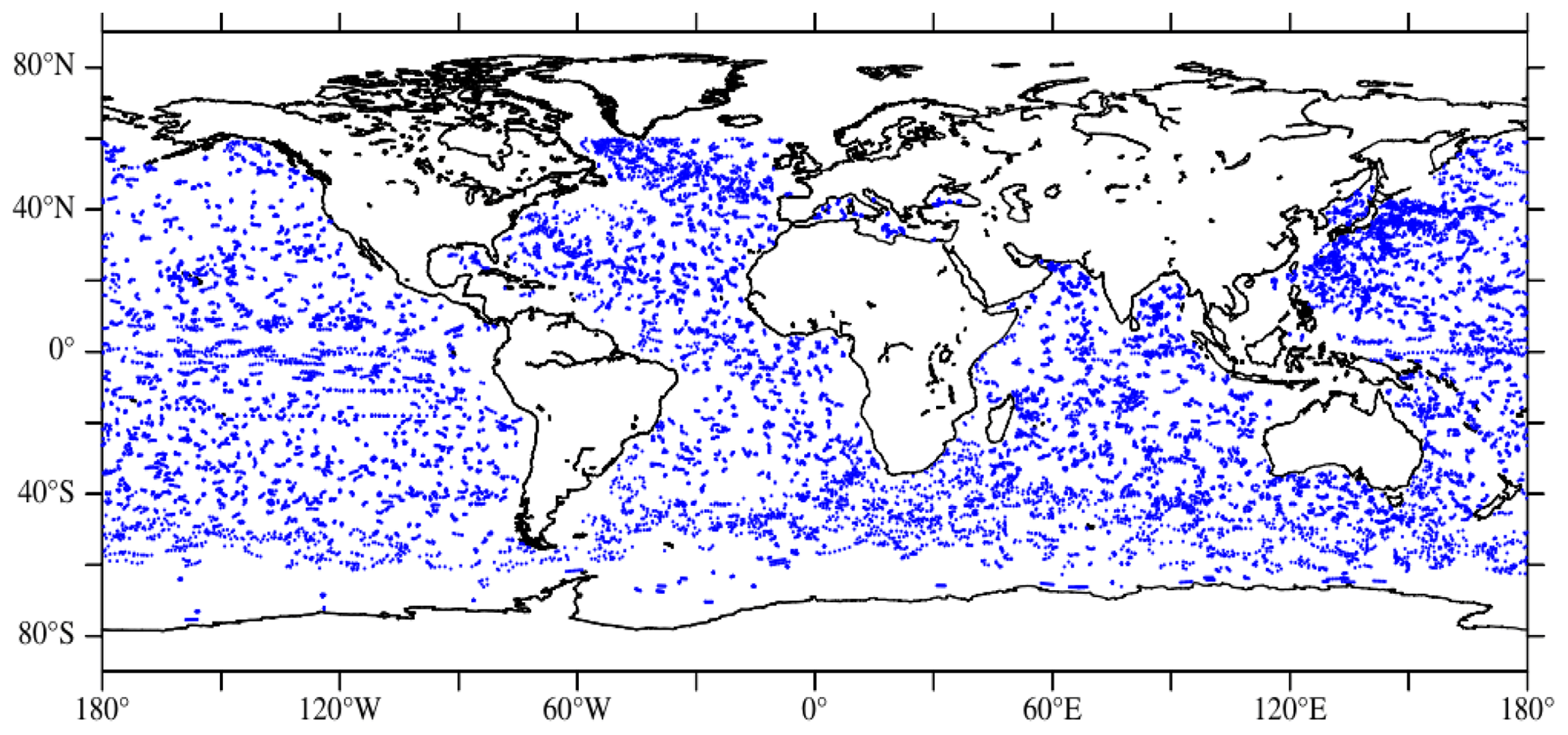
Figure 9Locations of ARGO profiles used in this study (period: 1 August–28 September 2011; 20 823 profiles in total).
3.5 ARGO profiles
To assess the model skill in capturing the vertical structures of temperature and salinity, we use all ARGO data in each ocean basin except the Arctic (Fig. 9).
The total number of ARGO profiles is around 330 on average per day in our simulation period. The model results are first interpolated from the surface to 2000 m to match the measuring range of ARGO. We follow the original ARGO data structure to divide our analysis into three different basins (Atlantic, Pacific, and Indian oceans), each including parts of the Southern Ocean. Due to the relatively small number of profiles (less than 30 per day) available near the surface (>6 m) in all basins, 0–6 m data are excluded to produce more reliable statistics.
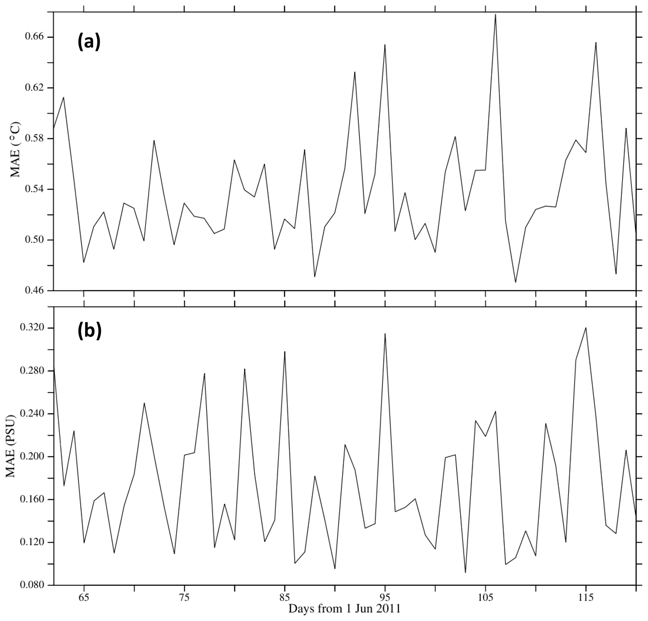
Overall, the modeled temperature and salinity profiles are satisfactory, with an MAE of ∼0.6 ∘C for temperature and ∼0.2 PSU for salinity (Fig. 10). Of all ocean basins, the Pacific Ocean has the smallest biases (Fig. 11). The simulated temperature in all basins tends to have a cold bias ( ∘C) near the surface, and biases below 200 m depth are smaller. The simulated salinity in all basins has a positive bias below 1400 m depth (Fig. 11), which is inherited from the initial condition. The good skill of the temperature and salinity profiles is also confirmed by the high correlation scores that exceed 0.9 most of the time (Fig. 12).
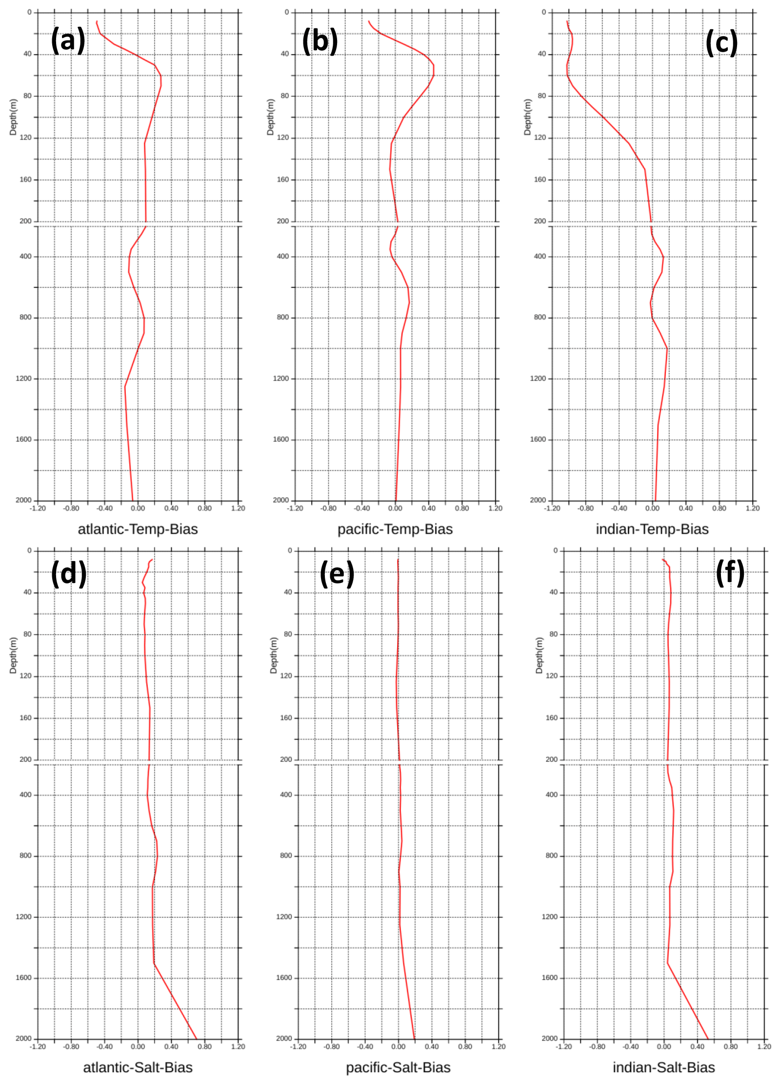
Figure 11Mean biases in each ocean basin: (a–c) temperature biases in the Atlantic, Pacific, and Indian oceans, respectively, and (d–f) salinity biases. Each plot is divided into two parts to clearly show the larger biases in the top 200 m depth.
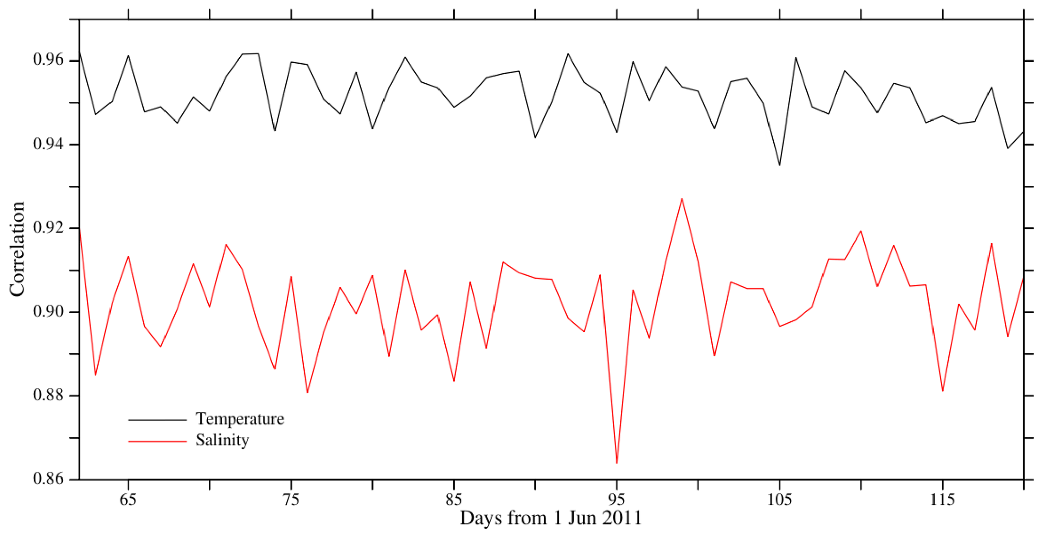
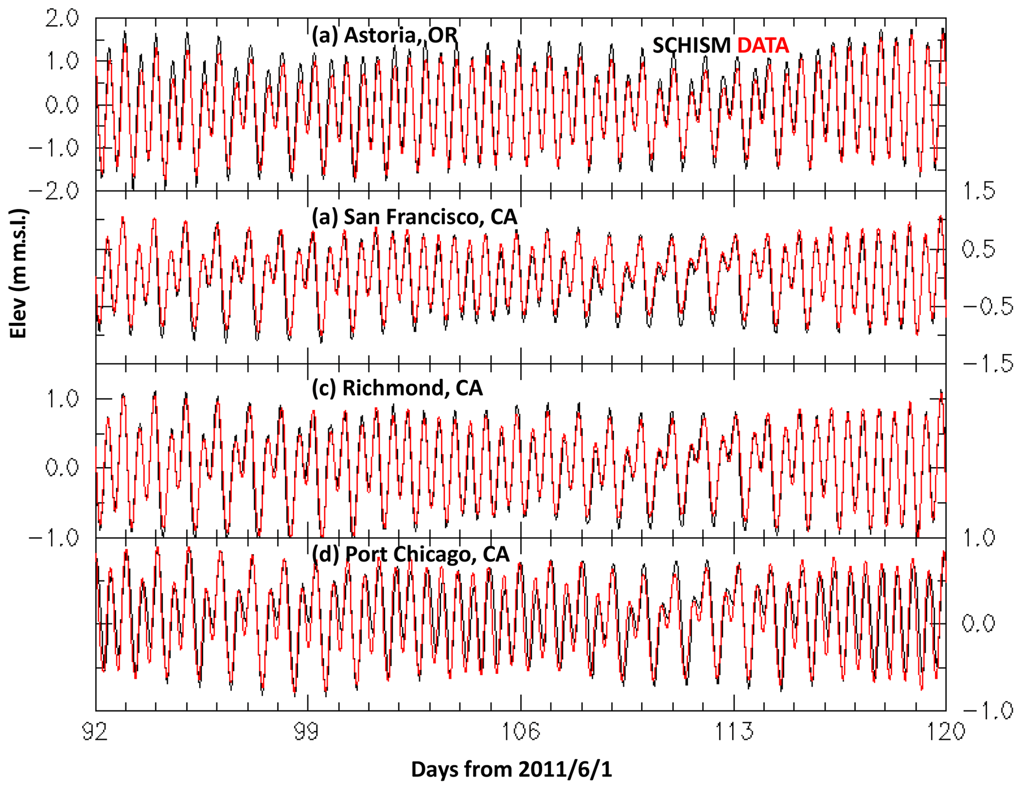
Figure 13Comparison of elevation at four tide gauges in the Columbia River and San Francisco Bay, USA. See Fig. 1c and d for gauge locations. The RMSEs are 18.7, 9.4, 8.3, and 15.4 cm; the correlation coefficients are 0.98, 0.98, 0.98, and 0.90; the Willmott skills are 0.98, 0.99, 0.99, and 0.95. Both the model and the data use NGVD29 as the vertical datum.
Calibrating a 3D baroclinic model like ours can be an expensive exercise, especially for 3D variables such as temperature, salinity, and velocity. However, since the focus of this paper is on the water surface elevation, we found through various sensitivity tests that the elevation results are sensitive to only a few parameters, including the bathymetry and bottom friction, because the thermo-steric contribution to elevation has been accounted for in the model. Compared to 2D models, the more complete physics embedded inside 3D models greatly simplifies the calibration process; e.g., the time-varying IT induced dissipation is already included in the model. This finding is consistent with our previous finding for a sub-domain of the US East Coast and the coast of the Gulf of Mexico (Huang et al., 2022). In this section we will show the sensitivity of the simulated elevations to the representation of the ice shelf effects in the Southern Ocean and exclusion of shallow areas.
A main novelty of our 3D UG model is its capability to seamlessly traverse scales from global oceans to very localized scales such as those found in estuaries and rivers. To the best of our knowledge, this capability has not been demonstrated before without resorting to grid nesting. Therefore, our model represents a major advancement in efficiently simulating global and local scales in a single UG model, thus allowing the interaction and connection among scales to be fully explored in our model. We demonstrate this potential here using two estuaries on the US West Coast as an example.
4.1 Southern Ocean: ice shelf effect
Bathymetry is known to play a pivotal role in the tidal and nontidal processes (Ye et al., 2018; Huang et al., 2022). As far as the global tide is concerned, one particularly important region is the Southern Ocean, which has an extensive distribution of ice shelves along the Antarctic coast. The existence of ice shelves effectively changes the local bathymetry, which affects tidal propagation locally and beyond (Blakely et al., 2022). Without accounting for those shelves, an erroneous amphidrome appears between the Drake Passage and Ross Sea (Fig. 3d vs 3a), and the amphidrome just east of the Ross Sea (Fig. 3a) is displaced westward (Fig. 3d). Other differences are also visible south of Australia and in the Weddell Sea (Fig. 3d vs 3a).
4.2 Feedback from shallow areas
To demonstrate the feedback from the shallow areas to the deeper ocean and its impact on global tidal energy dissipation, we removed all shallow areas with a depth of less than 50 m. Even though the shallow areas only account for ∼10 % of the total surface area (and even less in terms of volume), excluding the shallows significantly degrades the model skill in the deep ocean (e.g., the total RMSE is more than doubled from 5.4 to 11 cm for depths greater than 1 km). The lack of dissipation by the shallows is seen in the overestimated M2 amplitudes, especially in tidally energetic areas (e.g., European seas). The outcomes here are consistent with previous findings (e.g., A18) that shallows are important for the global tidal amplitudes. Without the shallows, most of the tidal energy would be reflected back into the deep ocean.
4.3 Into estuaries
As a proof of concept, we illustrate the model's potential in traversing from large oceanic scales to small estuarine scales using a few estuaries on the US West Coast as an example but leave detailed calibration and validation to future studies. Obviously, the calibration process will be expensive given the large mesh size used here. However, we show that with local mesh refinement and minimal calibration done in the current 3D model, the model is able to capture some small-scale processes.
The Columbia River and San Francisco Bay (SFB) are the two largest estuaries on the US West Coast (excluding Alaska) and are characterized as meso-tidal systems. The river discharge varies greatly between the two systems and over time. The Columbia River has a long-term mean flow of 2.5–11×103 m3 s−1 over a typical year (Bottom et al., 2005). SFB receives most of the freshwater inputs from the North Bay, which is connected to the Sacramento–San Joaquin River Delta, and the net delta outflow is smaller than the Columbia River (from ∼500 to 2000 m3 s−1). Both systems exhibit similar seasonality in the river flow, with the lowest flow occurring in late summer and highest flow during spring freshets. Due to the specificity of the forcings experienced by the two systems, the salt intrusion processes are quite different. The Columbia River estuary shows a strong spring–neap variation in the stratification and occasionally exhibits salt wedge conditions (Jay and Smith, 1990). In the MacCready–Geyer estuarine classification diagram, the Columbia River Estuary (CORIE) is classified as a “time-dependent salt wedge” system (Geyer and MacCready, 2004). The shorter shelf width near the CORIE makes it more susceptible to the prevailing coastal upwelling that is more common along the Oregon–Washington shelf. Previous modeling studies (Karna and Baptista, 2016) indicate that the Columbia River processes in particular are extremely challenging for numerical models. The SFB, on the other hand, represents a typical partially mixed estuary (Geyer and MacCready, 2004).
The total elevations at three NOAA tide gauges in SFB and one gauge in the CORIE are assessed in Fig. 13. Fortuitously, the vertical datum used in the model, NGVD29 (inherited from HYCOM), is close to the local mean seal level (MSL) used at these three gauges, and therefore no adjustment of the vertical datum is necessary. For other coastal regions (e.g., the US East Coast), the datum differences can be substantial, which calls for a geoid-based datum for regional and global tidal models (Jahanmard et al., 2021). With particular attention paid to the mesh representation near these two estuaries, the model is able to accurately capture the tidal and nontidal elevations in the two systems, as shown in Fig. 13, with RMSEs for the total elevations between 8.3 cm (at Richmond) and 18.7 cm (at Astoria) and the correlation coefficients and Wilmot scores all exceeding 0.95. As mentioned in Sect. 3.2, one major advantage of 3D models is their ability to better capture the NTR and thus TWL. Our experience suggests that with similar mesh refinement procedure, reliable DEMs, and some calibration with respect to the bottom drag coefficients, similar elevation skills can be obtained for other estuarine systems.
The Columbia River plume is a major coastal feature in the region, can extend hundreds of kilometers offshore (Baptista, 2006), and has a major impact on the ecosystem (Burla et al., 2010). The plume is highly dynamic and mostly wind driven but modulated by tides and river discharge (Burla et al., 2010). Figure 14 shows a “canonical” view of the plume when the wind forcing is weak or relaxed. The combination of the Coriolis force and inertial forces turns the plume northward with a coastally trapped jet in the north (in the form of Kelvin waves) and visible recirculation inside the freshwater bulge (Garcia-Berdeal et al., 2002). The model's ability to qualitatively capture the plume shape and extent is an important first step for further calibration.
Although a more careful validation against observations (including the vertical salinity profiles) is necessary to ascertain the model skill in capturing the smaller-scale 3D processes in estuaries, which would inevitably involve site-specific parameterization and calibration procedure, the preliminary results shown here are very promising and offer the potential to finally close the gap in simulating the global ocean–estuary–river–lake continuum. Note that the model does allow for specification of spatially variable parameterizations such as bottom drag and horizontal mixing schemes, which will be necessary in future calibration processes. On the other hand, the physical justifications of these choices, in the context of cross-scale processes from global oceans to estuaries and rivers, warrant further research; e.g., traditionally different horizontal mixing schemes have been used in the two regimes (Fringer et al., 2019).
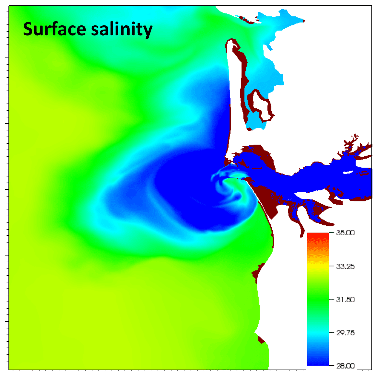
Figure 14Surface salinity plume near the Columbia River during a wind relaxation period.
We have developed a new 3D unstructured-grid (UG) model (SCHISM) for simulating the global ocean together with the coastal ocean and even estuaries in a single mesh, with high resolution applied in the latter. The simulated total elevation (including both tidal and nontidal components), temperature and salinity have been validated against satellite and in situ observation data. The simulated tide showed good skill, with a mean complex RMSE of 4.2 cm for M2 and 5.4 cm for the all major constituents at depths greater than 1 km. The nontidal residual assessed by the global tide gauge dataset (GESLA) had a mean RMSE of 7 cm. The mean MAE for SST excluding the Arctic is ∼0.8 ∘C.
For the first time ever, we demonstrated the potential for seamless simulation, without the need for grid nesting, from the global ocean to a few estuaries in the US West Coast at very high resolution. The model was able to accurately capture the total elevation and qualitatively capture the challenging salinity plume dynamics in the Columbia River.
Even though the 3D model is more expensive than 2D models, the improved accuracy and ease of calibration for the total water levels justify its cost; this advantage is in addition to the obvious benefits of being able to predict other 3D variables (velocity, temperature, salinity, etc). With adequate computational resources, the model can effectively serve as the engine of a global tide surge and even compound flooding forecasting framework. More meshing work and calibration will be required to further improve its accuracy in specific regions, and the UG nature of the model greatly simplifies the required work. In addition, a global tidal model would greatly benefit from transitioning from being a tidal-datum-based model to a geoid-based model to allow for more accurate simulation of the total elevation.
The source code of SCHISM v5.10.0 can be accessed from https://doi.org/10.5281/zenodo.6851013 (Zhang et al, 2022). An example of the 3D model setup can be found at https://doi.org/10.5281/zenodo.7779837 (Zhang et al., 2023).
All observation datasets used in this paper are publicly downloadable from the following web sites or DOIs. (1) OSTIA: https://doi.org/10.48670/moi-00165 (Good et al., 2020); (2) ARGO: https://doi.org/10.3389/fmars.2020.00700 (Wong et al., 2020); (3) GESLA: https://doi.org/10.5285/3b602f74-8374-1e90-e053-6c86abc08d39 (Woodworth et al., 2016b).
All authors contributed to writing of the paper. YJZ and WP worked on the model setup. TFM did analyses of the GESLA and altimetry. HCY and LC did the analyses for satellite SST and ARGO. SM advised and managed the project.
The contact author has declared that none of the authors has any competing interests.
Publisher's note: Copernicus Publications remains neutral with regard to jurisdictional claims in published maps and institutional affiliations.
This study was partially supported by NOAA Water Initiative (NA20NOS4200205). William Pringle was supported by the U.S. National Oceanic and Atmospheric Administration (NOAA) through a Virginia Institute of Marine Science sub-award under a Strategic Partnership Project agreement (A21162) to Argonne National Laboratory through U.S. Department of Energy contract no. DE-AC02-06CH11357. Simulations used in this paper were conducted using the following computational facilities:
-
William & Mary Research Computing (https://www.wm.edu/it/rc, last access: 2 May 2023);
-
the Extreme Science and Engineering Discovery Environment (XSEDE), which is supported by the National Science Foundation (grant no. OCI-1053575);
-
Texas Advanced Computing Center (TACC; grant no. EAR21010) at The University of Texas at Austin.
The ARGO data used are from the ARGO project (https://argo.ucsd.edu/data/acknowledging-argo/; https://doi.org/10.17882/42182).
This research has been supported by the National Ocean Service (grant no. NA20NOS4200205).
This paper was edited by Chanh Kieu and reviewed by Xianqing Lv and one anonymous referee.
Androsov, A., Fofonova, V., Kuznetsov, I., Danilov, S., Rakowsky, N., Harig, S., Brix, H., and Wiltshire, K. H.: FESOM-C v.2: coastal dynamics on hybrid unstructured meshes, Geosci. Model Dev., 12, 1009–1028, https://doi.org/10.5194/gmd-12-1009-2019, 2019.
Arbic, B. K., Wallcraft, A. J., and Metzger, E. J.: Concurrent simulation of the eddying general circulation and tides in a global ocean model, Ocean Model., 32, 175–187, https://doi.org/10.1016/j.ocemod.2010.01.007, 2010.
Arbic, B. K., Alford, M. H., Ansong, J. K., Buijsman, M. C., Ciotti, R. B., Farrar, J., Hallberg, R. W., Henze, C. E., Hill, C. N., Luecke, C. A., Menemenlis, D., Metzger, E., Müller, M., Nelson, A. D., Nelson, B. C., Ngodock, H. E., Ponte, R. M., Richman, J. G., Savage, A. C., Scott, R. B., Shriver, J. F., Simmons, H. L., Souopgui, I., Timko, P. G., Wallcraft, A. J., Zamudio, L., and Zhao, Z.: A Primer on Global Internal Tide and Internal Gravity Wave Continuum Modeling in HYCOM and MITgcm, New Frontiers In Operational Oceanography, 307–391, https://doi.org/10.17125/gov2018.ch13, 2018.
Baptista, A. M.: CORIE: the first decade of a coastal-margin collaborative observatory, Oceans 2006, MTS/IEEE, Boston, MA, 2006.
Baptista, A. M., Zhang, Y., Chawla, A., Zulauf, M. A., Seaton, C., Myers, E. P., Kindle, J., Wilkin, M., Burla, M., and Turner, P. J.: A cross-scale model for 3D baroclinic circulation in estuary-plume-shelf systems: II. Application to the Columbia River, Cont. Shelf Res., 25, 935–972, 2005.
Blakely, C. P., Ling, G., Pringle, W. J., Contreras, M. T., Wirasaet, D., Westerink, J. J., Moghimi, S., Seroka, G., Shi, L., Myers, E., Owensby, M., and Massey, C.: Dissipation and Bathymetric Sensitivities in an Unstructured Mesh Global Tidal Model, J. Geophys. Res.-Oceans, 127, e2021JC018178, https://doi.org/10.1029/2021JC018178, 2022.
Bottom, D. L., Simenstad, C. A., Burke, J., Baptista, A. M., Jay, D. A., Jones, K. K., Casillas, E., and Schiewe, M. H.: Salmon at river's end: The role of the estuary in the decline and recovery of Columbia River salmon, NOAA Tech. Memo., NMFS-NWFSC-68, 246 pp., U.S. Dept. of Commerce, 2005.
Burla, M., Baptista, A. M. Zhang, Y., and Frolov, S.: Seasonal and inter-annual variability of the Columbia River plume: a perspective enabled by multi-year simulation databases, J. Geophys. Res., 115, C00B16, https://doi.org/10.1029/2008JC004964, 2010.
Carrere, L., Lyard, F., Cancet, M., Guillot, A., and Roblou, L.: FES 2012: a new global tidal model taking advantage of nearly 20 years of altimetry, 20 Years of Progress in Radar Altimatry, 710, 13, 2013.
CoNED: Coastal National Elevation Database, https://www.usgs.gov/publications/coastal-national-elevation-database (last access: May 2023), 2022.
CUDEM: Continuously Updated Digital Elevation Model, https://coast.noaa.gov/htdata/raster2/elevation/NCEI_ninth_Topobathy_2014_8483/ (last access: May 2023), 2022.
Dai, A.: Hydroclimatic trends during 1950–2018 over global land, Clim. Dynam., 56, 4027–4049, https://doi.org/10.1007/s00382-021-05684-1, 2021.
Egbert, G. D. and Erofeeva, S. Y.: Efficient inverse modeling of barotropic ocean tides, J. Atmos. Ocean. Tech., 19, 183–204, 2002.
Egbert, R. D. and Ray, R. D.: Semi-diurnal and diurnal tidal dissipation from TOPEX/Poseidon altimetry, Geophys. Res. Lett., 30, 1907, https://doi.org/10.1029/2003GL017676, 2003.
Fringer, O. B., Dawson, C. N., He, R., Ralston, D. K., and Zhang, Y.: The future of coastal and estuarine modeling: Findings from a workshop, Ocean Model., 143, 101458, https://doi.org/10.1016/j.ocemod.2019.101458, 2019.
Garcia-Berdeal, I., Hickey, B. M., and Kawase, M.: Influence of wind stress and ambient flow on a high discharge river plume, J. Geophys. Res. 107, 3130, https://doi.org/10.1029/2001JC000932, 2002.
Garner, S. T.: A topographic drag closure built on an analytical base flux, J. Atmos. Sci., 62, 2302–2315, https://doi.org/10.1175/JAS3496.1, 2005.
GEBCO Compilation Group: GEBCO 2019 Grid, https://doi.org/10.5285/836f016a-33be-6ddc-e053-6c86abc0788e, 2019.
Geyer, W. R. and MacCready, P.: The Estuarine Circulation, Annu. Rev. Fluid Mech., 46, 175–197, 2004.
Good, S., Fiedler, E., Mao, C., Martin, M. J., Maycock, A., Reid, R., Roberts-Jones, J., Searle, T., Waters, J., While, J., and Worsfold, M.: The Current Configuration of the OSTIA System for Operational Production of Foundation Sea Surface Temperature and Ice Concentration Analyses, Remote Sens., 12, 720, https://doi.org/10.3390/rs12040720, 2020 (data available at: https://doi.org/10.48670/moi-00165).
Huang, W., Ye, F., Zhang, Y., Park, K., Du, J., Moghimi, S., Myers, E., Pe'eri, S., Calzada, J. R., Yu, H. C., Nunez, K., and Liu, Z.: Compounding factors for extreme flooding around Galveston Bay during Hurricane Harvey, Ocean Model., 158, 101735, https://doi.org/10.1016/j.ocemod.2020.101735, 2021.
Huang, W., Zhang, Y., Wang, Z., Ye, F., Moghimi, S., Myers, E., and Yu, H.: Tidal simulation revisited, Ocean Dynam., 72, 187–205, https://doi.org/10.1007/s10236-022-01498-9, 2022.
Holt, J., Hyder, P., Ashworth, M., Harle, J., Hewitt, H. T., Liu, H., New, A. L., Pickles, S., Porter, A., Popova, E., Allen, J. I., Siddorn, J., and Wood, R.: Prospects for improving the representation of coastal and shelf seas in global ocean models, Geosci. Model Dev., 10, 499–523, https://doi.org/10.5194/gmd-10-499-2017, 2017.
Jahanmard, V., Delpeche-Ellmann, N., and Ellmann, A.: Realistic dynamic topography through coupling geoid and hydrodynamic models of the Baltic Sea, Cont. Shelf Res., 222, 104421, https://doi.org/10.1016/j.csr.2021.104421, 2021.
Jay, D. A. and Smith, J. D.: Circulation, density distribution and nea-spring transitions in the Columbia river estuary, Prog. Oceanogr., 25, 81–112, 1990.
Karna, T. and Baptista, A.M .: Evaluation of a long-term hindcast simulation for the Columbia River estuary, Ocean Model., 99, 1–14, 2016.
Logemann, K., Linardakis, L., and Korn, P.: Global tide simulations with ICON-O: testing the model performance on highly irregular meshes, Ocean Dynam., 71, 43–57, https://doi.org/10.1007/s10236-020-01428-7, 2021.
Lyard, F. H., Allain, D. J., Cancet, M., Carrère, L., and Picot, N.: FES2014 global ocean tide atlas: design and performance, Ocean Sci., 17, 615–649, https://doi.org/10.5194/os-17-615-2021, 2021.
Munk, W. H. and Wunsch, C.: Abyssal recipes II: energetics of tidal and wind mixing, Deep-Sea Res. Pt. I, 45, 1977–2010, https://doi.org/10.1016/S0967-0637(98)00070-3, 1998.
Pawlowicz, R., Beardsley, R., and Lentz, S.: Classical tidal harmonic analysis including error estimates in MATLAB using T_TIDE, Comput. Geosci., 28, 929–937, 2002.
Pickering, M. D., Horsburgh, K. J., Blundell, J. R., Hirschi, J. J.-M. Nicholls, R. J., Verlaan, M., and Wells, N. C.: The impact of future sea-level rise on the global tides, Cont. Shelf Res., 142, 50–68, 2017.
Pringle, W. J., Gonzalez-lopez, J., Joyce, B., Westerink, J. J., and van der Westhuysen, A. J.: Baroclinic Coupling Improves Depth-Integrated Modeling of Coastal Sea Level Variations around Puerto Rico and the U.S. Virgin Islands, J. Geophys. Res.-Oceans, 124, 2196–2217, https://doi.org/10.1029/2018JC014682, 2019.
Pringle, W. J., Wirasaet, D., Roberts, K. J., and Westerink, J. J.: Global storm tide modeling with ADCIRC v55: unstructured mesh design and performance, Geosci. Model Dev., 14, 1125–1145, https://doi.org/10.5194/gmd-14-1125-2021, 2021.
Ringler, T., Petersen, M., Higdon, R. L., Jacobsen, D., Jones, P. W., and Maltrud, M.: A multi-resolution approach to global ocean modeling, Ocean Model., 69, 211–232, https://doi.org/10.1016/j.ocemod.2013.04.010, 2013.
Savage, A. C., Arbic, B. K., Alford, M. H., Ansong, J. K., Farrar, J. T., Menemenlis, D., O'Rourke, A. K., Richman, J. G., Shriver, J. F., Voet, G., Wallcraft, A. J., and Zamudio, L.: Spectral decomposition of internal gravity wave sea surface height in global models, J. Geophys. Res.-Oceans, 122, 7803–7821, https://doi.org/10.1002/2017JC013009, 2017.
Schaffer, J., Timmermann, R., Arndt, J. E., Kristensen, S. S., Mayer, C., Morlighem, M., and Steinhage, D.: A global, high-resolution data set of ice sheet topography, cavity geometry, and ocean bathymetry, Earth Syst. Sci. Data, 8, 543–557, https://doi.org/10.5194/essd-8-543-2016, 2016.
Schindelegger, M., Green, J. A., Wilmes, S. B., and Haigh, I. D.: Can We Model the Effect of Observed Sea Level Rise on Tides?, J. Geophys. Res.-Oceans, 123, 4593–4609, https://doi.org/10.1029/2018JC013959, 2018.
Stepanov, V. N. and Hughes, C. W.: Parameterization of ocean self-attraction and loading in numerical models of the ocean circulation, J. Geophys. Res.-Oceans, 109, 1–11, https://doi.org/10.1029/2003jc002034, 2004.
Umlauf, L. and Burchard, H.: A generic length-scale equation for geophysical turbulence models, J. Mar. Res., 6, 235–265, 2003.
Wang, P., Bernier, N. B., and Thompson, K. R.: Adding baroclinicity to a global operational model for forecasting total water level: Approach and impact, Ocean Model., 174, 102031, https://doi.org/10.1016/j.ocemod.2022.102031, 2022.
Wang, X., Chao, Y., Shum, C. K., Yi, Y., and Fok, H. S.: Comparison of two methods to assess ocean tide models, J. Atmos. Ocean. Tech., 29, 1159–1167, 2012.
Willmott, C. J.: On the validation of models, Phys. Geogr., 2, 184–194, 1981.
Wong, A., Wijffels, S.E., Riser, S.C., Pouliquen, S., Hosoda, S., Roemmich, D., Gilson, J., Johnson, G.C., Martini, K., Murphy, D.J., Scanderbeg, M., Bhaskar, T., Buck, J., Merceur, F., Carval, T., Maze, G., Cabanes, C., André, X,, Poffa, N., Yashayaev, I., Barker, P.M., Guinehut, S., Belbéoch, M., Ignaszewski. M., Baringer, M.O., Schmid, C., Lyman, J.M., McTaggart, K.E., Purkey, S.G., Zilberman, N., Alkire, M.B., Swift, D., Owens, W.B., Jayne, S.R., Hersh, C., Robbins, P., West-Mack, D., Bahr, F., Yoshida, S., Sutton, P., Cancouët, R., Coatanoan, C., Dobbler, D., Juan, A.G., Gourrion, J., Kolodziejczyk, N., Bernard, V., Bourlès, B., Claustre, H., D'Ortenzio, F., Le Reste, S., Le Traon, P.-Y., Rannou, J.-P., Saout-Grit, C., Speich, S., Thierry, V., Verbrugge, N., Angel-Benavides, I.M., Klein, B., Notarstefano, G., Poulain, P.-M., Vélez-Belchí, P., Suga, T., Ando, K., Iwasaska, N., Kobayashi, T., Masuda, S., Oka, E., Sato, K., Nakamura, T., Sato, K., Takatsuki, Y., Yoshida, T., Cowley, R., Lovell, J.L., Oke, P.R., van Wijk, E.M., Carse, F., Donnelly, M., Gould, W.J., Gowers, K., King, B.A., Loch, S.G., Mowat, M., Turton, J., Rama, R., Ravichandran, M., Freeland, H.J., Gaboury, I., Gilbert, D., Greenan, B., Ouellet, M., Ross, T., Tran, A., Dong, M., Liu, Z., Xu, J., Kang, K., Jo, H., Kim, S.-D., and Park, H.-M.: Argo Data 1999–2019: Two Million Temperature-Salinity Profiles and Subsurface Velocity Observations From a Global Array of Profiling Floats, Front. Mar. Sci., 7, 700, https://doi.org/10.3389/fmars.2020.00700, 2020.
Woodworth, P. L., Hunter, J. R., Marcos, M., Caldwell, P., Menéndez, M., and Haigh, I.: Towards a global higher-frequency sea level dataset, Geosci. Data J., 3, 50–59, 2016a.
Woodworth, P. L., Hunter, J. R., Marcos Moreno, M., Caldwell, P. C., Menendez, M., and Haigh, I. D.: GESLA (Global Extreme Sea Level Analysis) high frequency sea level dataset – Version 2, British Oceanographic Data Centre – Natural Environment Research Council [data set], UK, https://doi.org/10.5285/3b602f74-8374-1e90-e053-6c86abc08d39, 2016b.
Ye, F., Zhang, Y., Wang, H., Friedrichs, M. A. M., Irby, I. D., Alteljevich, E., Valle-Levinson, A., Wang, Z., Huang, H., Shen, J., and Du, J.: A 3D unstructured-grid model for Chesapeake Bay: importance of bathymetry, Ocean Model., 127, 16–39, 2018.
Ye, F., Zhang, Y., He, R., Wang, Z., Wang, H. V., and Du, J.: Third-order WENO transport scheme for simulating the baroclinic eddying ocean on an unstructured grid, Ocean Model., 143, 101466, https://doi.org/10.1016/j.ocemod.2019.101466, 2019.
Ye, F., Zhang, Y., Yu, H., Sun, W., Moghimi, S., Myers, E.P., Nunez, K., Zhang, R., Wang, H. V., Roland, A., Martins, K., Bertin, X., Du, J., and Liu, Z.: Simulating storm surge and compound flooding events with a creek-to-ocean model: importance of baroclinic effects, Ocean Model., 145, 101526, https://doi.org/10.1016/j.ocemod.2019.101526, 2020.
Ye, F., Huang, W., Zhang, Y. J., Moghimi, S., Myers, E., Pe'eri, S., and Yu, H.-C.: A cross-scale study for compound flooding processes during Hurricane Florence, Nat. Hazards Earth Syst. Sci., 21, 1703–1719, https://doi.org/10.5194/nhess-21-1703-2021, 2021.
Zhang, Y., Ateljevich, E., Yu, H-C., Wu, C.-H., and Yu, J. C. S.: A new vertical coordinate system for a 3D unstructured-grid model, Ocean Model., 85, 16–31, 2015.
Zhang, Y., Ye, F., Stanev, E. V., and Grashorn, S.: Seamless cross-scale modeling with SCHISM, Ocean Model., 102, 64–81, https://doi.org/10.1016/j.ocemod.2016.05.002, 2016.
Zhang, Y., Ye, F., Yu, H., Sun, W., Moghimi, S., Myers, E.P., Nunez, K., Zhang, R., Wang, H.V., Roland, A., Du, J., and Liu, Z.: Simulating compound flooding events in a hurricane, Ocean Dynam., 70, 621–640, https://doi.org/10.1007/s10236-020-01351-x, 2020.
Zhang, Y. J., Wang, Z. G., Ye, F., Cai, C., Lemmen, C., Khan, J.U., Yu, H.C., Wang, Q., Calzada, J. R., Mentaschi, L., Seaton, C., Nam, K., Martins, K., Shu, Q., Breyiannis, B., Trenham, C., Ateljecvich, E., Tran, H. Q., Clements, J., Huang, W., and Pezerat, M.: schism-dev/schism: (v5.10.0), Zenodo [code], https://doi.org/10.5281/zenodo.6851013, 2022.
Zhang, Y. J., Fernandez-MontBlanc, T., Pringle, W., Yu, H.-C., Cui, L., and Moghimi, S.: Global seamless tidal simulation using a 3D unstructured-grid model, Geoscientific Model Development, Zenodo [code], https://doi.org/10.5281/zenodo.7779837, 2023.
seamlesssimulation, on a single mesh, from the global ocean to a few estuaries along the US West Coast. The model can serve as the backbone of a global tide surge and compound flooding forecasting framework.