the Creative Commons Attribution 4.0 License.
the Creative Commons Attribution 4.0 License.
 | 09 May 2023
ChemicalDrift 1.0: an open-source Lagrangian chemical-fate and transport model for organic aquatic pollutants
Loris Calgaro
Knut-Frode Dagestad
Christian Ferrarin
Antonio Marcomini
Øyvind Breivik
Lars Robert Hole
A new model for transport and fate of chemicals in the aquatic environment is presented. The tool, named ChemicalDrift, is integrated into the open-source Lagrangian framework OpenDrift and is hereby presented for organic compounds. The supported chemical processes include the degradation, the volatilization, and the partitioning between the different phases that a target chemical can be associated with in the aquatic environment, e.g. dissolved, bound to suspended particles, or deposited to the seabed sediments. The dependencies of the chemical processes on changes in temperature, salinity, and particle concentration are formulated and implemented. The chemical-fate modelling is combined with wide support for hydrodynamics by the integration within the Lagrangian framework which provides e.g. advection by ocean currents, diffusion, wind-induced turbulent mixing, and Stokes drift generated by waves. A flexible interface compatible with a wide range of available metocean data is made accessible by the integration, making the tool easily adaptable to different spatio-temporal scales and fit for modelling of complex coastal regions. Further inherent capabilities of the Lagrangian approach include the seamless tracking and separation of multiple sources, e.g. pollutants emitted from ships or from rivers or water treatment plants. Specific interfaces to a dataset produced by a model of emissions from shipping and to an unstructured-grid oceanographic model of the Adriatic Sea are provided. The model includes a database of chemical parameters for a set of poly-aromatic hydrocarbons and a database of emission factors for different chemicals found in discharged waters from sulfur emission abatement systems in marine vessels. A post-processing tool for generating mean concentrations of a target chemical, over customizable spatio-temporal grids, is provided. Model development and simulation results demonstrating the functionalities of the model are presented, while tuning of parameters, validation, and reporting of numerical results are planned as future activities. The ChemicalDrift model flexibility, functionalities, and potential are demonstrated through a selection of examples, introducing the model as a freely available and open-source tool for chemical fate and transport that can be applied to assess the risks of contamination by organic pollutants in the aquatic environment.
- Article
(7289 KB) - Full-text XML
- BibTeX
- EndNote


The negative effects of chemical pollution on the environment and human health have long been established (Naidu et al., 2021), but only more recently has the need for integrated strategies and solutions for the simultaneous management of multiple stressors been widely recognized (Pirotta et al., 2022). In fact, one of the main challenges in assessing the impact of anthropogenic stressors on the environment, and especially on aquatic ecosystems, is to estimate the exposure to these contaminants while also keeping track of their origin, in particular when multiple sources of chemical pollution are present.
Lagrangian models (van Sebille et al., 2018) offer the possibility of investigating the transport of chemicals without losing information on their origin, thus facilitating the assessment of the contribution each source has to the overall exposure of the target ecosystem. Furthermore, since their spatial resolution is not inherently limited to the resolution of Eulerian grid boxes and no grid generation is required (Azarpira et al., 2021), Lagrangian models are suitable for studying areas with complex geometries such as coasts, lagoons and archipelagos. The capabilities of these models to predict the transport of chemicals and particles emitted into the atmosphere by a variety of sources (e.g. industrial installations, Hirdman et al., 2010; Lee et al., 2014, nuclear accidents, Becker et al., 2007; Draxler et al., 2015, and volcanic eruptions, Prata et al., 2007; D'Amours et al., 2010) have been widely studied (Onink et al., 2021). On the other hand, the potential of Lagrangian models applied to the fate and transport of organic chemicals in the water compartment is not fully investigated.
It is recognized that coastal environments are of particular concern due to the presence of multiple stressors (e.g. wastewater discharge, soil and sediment contamination, agricultural and municipal run-off and combustion of fossil fuels by civil and industrial activities) (Danovaro and Boero, 2019; Szymczycha et al., 2019; Calgaro et al., 2019, 2021), posing a risk to the ecosystem and human health due to water and air contamination. An additional specific stressor is represented by emissions of SOx, NOx and other airborne contaminants (e.g. particulate matter and polyaromatic hydrocarbons) from shipping activity, which has been shown to significantly degrade air quality (Zhang et al., 2021), especially in areas characterized by high traffic such as ports and shipping lanes. For these reasons, the International Maritime Organization (IMO), starting from 1 January 2020, has introduced new global regulations limiting the sulfur content of fossil fuels to a maximum of 0.50 % weight / weight (), unless they are fitted with a suitable exhaust-gas-cleaning system (“scrubbers”) (Vedachalam et al., 2022). Furthermore, the more stringent limit of 0.10 % sulfur has been applied to especially sensitive areas (i.e. emission control areas, ECAs) like the Baltic Sea, the North Sea and the US coasts (Chang et al., 2018). Plans to include other areas in the ECA list, like the Mediterranean Sea, are under discussion (Testa, 2020).
The scrubbing process is implemented by leading the exhaust gas through a fine-water mist where SOx and NOx are dissolved together with particulate matter, metals and organic compounds (Lunde Hermansson et al., 2021), and thus large volumes of toxic (Turner et al., 2017) and highly acidified effluents (Turner et al., 2018) (where several pollutants, e.g. Cu, Pb, Hg, V, Zn, As, Ni and polyaromatic hydrocarbons (PAHs), have been detected) are produced and discharged into the sea. Moreover, due to the increase in shipping traffic predicted for the next decades (Sardain et al., 2019), it is crucial to develop methods and tools to investigate the impact of scrubber use on the marine ecosystem in relation to other sources of chemical pollution.
The present work is carried out under the scope of the Horizon 2020 EMERGE project, which aims to develop an integrated modelling framework to assess the combined impact of shipping emission-control options on the aquatic and atmospheric environment. Utilizing the open-source Lagrangian framework OpenDrift (Dagestad et al., 2018), a new model for chemical transport and fate of aquatic pollutants, named ChemicalDrift, has been developed and is hereby presented and demonstrated.
This article is organized as follows: the relevant chemical processes implemented in ChemicalDrift are presented and formulated in Sect. 2; the set of inputs utilized in this work, including metocean forcing data, chemical parameters for the studied pollutants, and emission source data, are presented in Sect. 3, and a selection of demonstrative examples are presented in Sect. 4. Planned future developments and conclusions are summarized in Sect. 5.
The new module ChemicalDrift is presented in this section, supported by a detailed description of the modelled chemical processes. The module is coded in Python and integrated into the open-source Lagrangian framework OpenDrift (Dagestad et al., 2018), where the fundamental physical processes of advection and diffusion as well as atmospheric and oceanographic forcing were previously implemented. The OpenDrift framework already contains a module for oil pollution, OpenOil (Dagestad et al., 2018), which has been validated and used for simulations of oil spills (Röhrs et al., 2018; Brekke et al., 2021; Hole et al., 2021), i.e. mixtures of petroleum products modelled as oil droplets or oil/water emulsions in the water column. The module presented here has a different target, being intended for simulations of dispersion of specific single chemicals, which might be hazardous contaminants even at very low concentrations in the water column or in the sediment layer, and includes a new implementation of the relevant chemical processes.
Only the chemistry of non-ionizable organic compounds is described in this work, since the chemistry of metals has already been implemented in the Radionuclides OpenDrift module (Simonsen et al., 2019a), which is integrated into ChemicalDrift.
The reactions implemented in ChemicalDrift include a partitioning scheme between the different phases that a target chemical can be associated with within the aquatic environment, the degradation of organic chemicals in the water column and in the sediments and the volatilization of dissolved chemicals from the water to the atmosphere. The dependencies of the each reaction on temperature and salinity changes are described and implemented based on the scientific literature. Sedimentation and resuspension are also presented in this section since these physical processes are strongly related to the chemical-phase partitioning.
2.1 Dynamic partitioning between compartments
Chemicals in the aquatic environment can be associated with different components of this medium (i.e. dissolved in the water or bound to dissolved organic carbon (DOC), suspended particle matter (SPM) or sediments) and are thereby exposed to different physical and chemical processes. For example, dissolved chemicals will be transported by advection due to water currents and by turbulent diffusion processes, such as wind-induced vertical mixing, while chemicals adsorbed to solid particles will also be affected by gravity and might sink towards the sea floor. Furthermore, the different distributions between dissolved and bound chemicals will also influence its availability to degradation processes like hydrolysis, biodegradation and photolysis. In computational models it is therefore crucial to process each of these components in distinct compartments.
In ChemicalDrift, each Lagrangian element represents a given mass of a target chemical, and the partitioning between the media components is implemented by assigning each element to a single corresponding model compartment. The partitioning is carried out dynamically, as opposed to a simpler steady-state approach, and transfer rates between compartments are calculated and applied at each time step. The dynamic approach is fit for the changing environmental conditions each Lagrangian element is exposed to (i.e. water temperature, salinity, SPM and DOC concentration), as it is transported in the media.
The dynamic partitioning scheme used in ChemicalDrift was first introduced by Periáñez and Elliott (2002) and implemented in the OpenDrift Radionuclides module (Simonsen et al., 2019a, b), where it was applied to metals. In this work, several adaptations were made to expand its applicability to organic chemicals and consider the influence of temperature and salinity changes on the transfer rates.
The main phases considered in the algorithm (Fig. 1) include (i) dissolved in the water fraction, (ii) adsorbed to the SPM fraction, and (iii) the sediment fraction. The sediment fraction includes both the chemical adsorbed to solid particles that have settled to the sea floor and the chemical dissolved in the interstitial water present in the space between the settled particles. Optional model compartments can also be activated. The chemical can also be modelled as adsorbed to DOC and form other aggregates that will be subjected to sinking (i.e. the DOC phase). Adsorption to solid particles can be treated as a two-step process where the diffusion of the chemical within the particle is also considered (i.e. a slowly reversible fraction, SR) for both SPM and sediments. Finally, an optional compartment for buried sediments is implemented, representing a sink for the target chemical that is progressively buried below layers of overlying sediments and is therefore not available for exchanges with the water column.
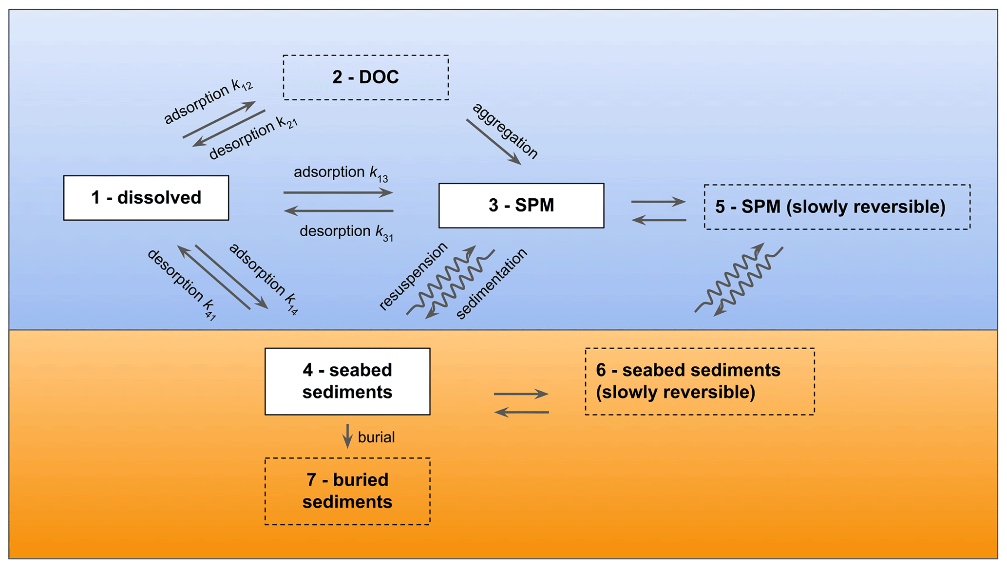
Figure 1The model compartments implemented in ChemicalDrift and the corresponding exchange processes and transfer rates adapted from Simonsen et al. (2019a). The default (dissolved, adsorbed to SPM and sediments) compartments are indicated with solid contours. Optional compartments are depicted with dashed contours.
2.1.1 Adsorption and desorption rates
Transfer rates are calculated by adapting the equations described by Simonsen et al. (2019a) and are applied using the approach explained in Sect. 2.1.2 for estimating the adsorption and desorption kinetic constants, kads (L kg−1 h−1) and kdes (h−1).
Transfer rates from the dissolved phase to the DOC, SPM and sediment compartments (i.e. k12, k13 and k14) and the corresponding desorption rates (i.e. k21, k31 and k41) are given by
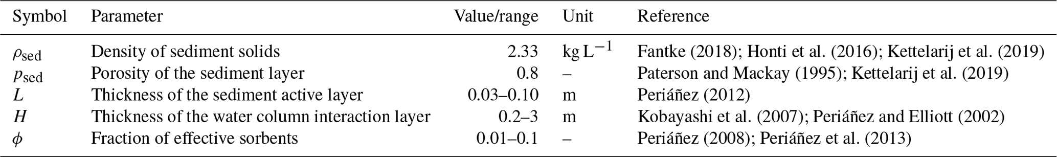
Here the indices refer to the numbering illustrated in Fig. 1: CDOC is the concentration of DOC in the water column (kg L−1), CSPM is the concentration of SPM in the water column (kg L−1), ρsed is the density of sediment solids (kg m−3), psed is the porosity of the sediments, L (m) is thickness of the sediment layer which interacts with the water column, H (m) gives the thickness of the water layer above the sea bottom that interacts with the sediment, ϕ is the fraction of effective sorbents considering that a fraction of the sediment particle surface may be unavailable for sorption–desorption interactions due to neighbouring sediment particles and δ is the logical variable which ensures that only the chemicals in the seabed interaction layer are able to adsorb to sediments and is set to 1 when the distance to the seabed is less than H and 0 elsewhere. Default values or typical ranges are summarized in Table 1. The concentrations CDOC and CSPM are provided as modelled or experimentally derived data fields. If only 2-D surface data are available, the vertical profiles are estimated assuming a constant concentration in the mixed layer (equal to the surface values) and exponentially decreasing with depth below the mixed layer, with user-definable constants, in accordance with the observations of biogeochemical Argo float measurements reported by Galí et al. (2022).
Fantke (2018); Honti et al. (2016); Kettelarij et al. (2019)Paterson and Mackay (1995); Kettelarij et al. (2019)Periáñez (2012)Kobayashi et al. (2007); Periáñez and Elliott (2002)Periáñez (2008); Periáñez et al. (2013)Table 1Parameters for the calculation of sediment-layer adsorption and desorption rates.
The stochastic method for calculating the probability of phase change between model compartments given the time step and the transfer rates is described by Periáñez and Elliott (2002).
2.1.2 General estimation of kads and kdes for organic chemicals
The partitioning of organic chemicals to organic carbon has been reported as involving rapid adsorption to particle surfaces, followed by slow movement into, and out of, organic matter and porous aggregates (Karickhoff and Morris, 1985), thus determining the time needed for the attainment of equilibrium (Park and Clough, 2014).
The solid–water partition coefficient Kd (L kg−1) is the ratio between the adsorption and desorption kinetic constants:
Given this context, Karickhoff and Morris (Karickhoff and Morris, 1985; Site, 2001) found the reciprocal of kdes to be a linear function of Kd over 3 orders of magnitude (r2=0.87), following . Using this approximation and the definition of Kd, the adsorption and desorption kinetic constants can be estimated as
The value of Kd for a given chemical in the aquatic environment can be subjected to significant changes due to e.g. temperature, salinity, SPM and DOC concentration variations and pH; therefore, the use of experimental local measurements of Kd is recommended. However, if such data are not available, the model will estimate the Kd as described below.
For organic chemicals it is assumed that the organic carbon fraction of solid particles (i.e. suspended particle matter and sediments) is almost entirely responsible for their sorbing capacity, and therefore Kd can be expressed as the product of a water–organic carbon partition coefficient (i.e. KOC – L kg) and the organic carbon content of the dry matter (fOC – gOC g−1).
Typical values for fOC are in the range 0.01–0.10 gOC g−1 (Seiter et al., 2004).
Relationships between KOC and the octanol–water partition coefficient KOW (L kg−1) are available from previous studies. In the case of non-ionizing organic chemicals, the following formulations reported by Park and Clough (2014) are used to estimate KOC for SPM and DOC, respectively.
2.1.3 Effect of temperature and salinity on the solid–water partition coefficient
Experimental values of KOC and Kd are usually obtained at standard or ambient temperature and for fresh water, but temperature and salinity variations have been shown to have a strong impact on the adsorption of chemicals to SPM, DOC, and sediments. The following equation and correction factors are applied to obtain to obtain the solid–water partition coefficient Kd(T,S) for a desired value of temperature T (K) and salinity S (PSU) based on a known reference value Kd(Tref,0):
where kS is the Setschenow (salting-out) constant in seawater of the non-ionizable organic chemical with respect to the specific salt considered (L mol−1), and Csalt is the molar concentration of the salts in solution (mol L−1). Salt concentration is calculated starting from salinity considering the molecular weight of seawater salt, MolWtsalt=68.35 g mol−1 (Schwarzenbach et al., 2016), and the water density, ρ.
The correction factor for temperature is based on the Arrhenius equation where ΔH (J mol−1) is the enthalpy of adsorption for the given chemical and R is the universal gas constant (R=8.3145 J mol−1 K−1). The model utilizes distinct enthalpies for DOC and SPM, indicated as ΔHKOC,DOC and ΔHKOC,SPM, respectively.
2.1.4 Sedimentation and resuspension
Particle sedimentation and resuspension dynamics in ChemicalDrift are partly based on methods previously implemented in other OpenDrift modules. The vertical motion of Lagrangian elements representing dissolved chemicals or chemicals adsorbed to DOC is calculated as for a passive tracer by adding vertical currents (typically small compared to the other terms) to the vertical mixing associated with wind-induced or background turbulent diffusion.
Lagrangian elements associated with SPM are also affected by gravity and will sink towards the sea floor, and hence a third component has to be added to calculate the vertical motion. This term is referred to as the terminal velocity and is calculated from Stokes' law (Stokes, 1851), assuming the particles to be spherical with known density and diameter (Sundby, 1983). Empirical relationships are utilized to update the water density (Fofonoff and Millard Jr, 1983) and viscosity (Ådlandsvik, 2000; Myksvoll et al., 2013) based on T and S as the elements sink.
When sinking particles reach the sea floor, the chemical elements are transferred to the sediment-layer compartments and thus can be subjected to either sediment burial or resuspension. Resuspension occurs when the horizontal current at the bottom is greater than a given threshold vcrit. Resuspended elements are lifted from the previous sea-floor depth zmin (depth below sea level, negative) to a depth , where zres is the resuspension depth, zres,unc is the resuspension depth uncertainty and is a randomly generated number from a normal distribution with zero mean and standard deviation zres,unc (Simonsen et al., 2019a).
2.2 Degradation
Organic chemicals in the aquatic environment can be degraded due to various processes, such as biodegradation, photodegradation and hydrolysis. Modelling each of these reactions separately requires a large amount of information on the environmental behaviour of the target chemical and on the characteristics of the selected study area. Since these data are typically difficult to obtain with sufficient accuracy for a wide range of chemicals and case-study regions, a simpler approach is implemented in the current version of ChemicalDrift: degradation is implemented considering distinct overall reaction rates for the water column (subscript Wtot) and the sediments (subscript Stot) and modelled as a first-order kinetic decay of the mass associated with each Lagrangian element; in detail, overall degradation rate constants k or the corresponding half-lives can be obtained experimentally without separating the effects of the three sub-processes. The mass mi(t) of each Lagrangian chemical element is calculated at each time step applying
where kW tot is the overall (total) degradation constant for the chemical either dissolved in the water column or adsorbed to dissolved organic carbon/matter, kS tot is the overall degradation constant for chemicals in the sediment layer and Δt is the time-step interval. As reported by, among others, Kettelarij et al. (2019), it is assumed that degradation of chemicals adsorbed to suspended particles can be neglected. Degradation rate constants can be specified directly or calculated from the corresponding half-life constants , applying . Furthermore, the effect of temperature is considered by applying to each degradation rate constant a correction factor calculated by applying the Arrhenius equation as in Eq. (10) using the reference temperature (i.e. Tref W tot and Tref S tot) and enthalpy (i.e. ΔHW tot and ΔHS tot) associated with each process. Salinity has also been demonstrated to have an impact on the microbial populations responsible for the biodegradation of organic chemicals, but since the modelling of these effects would require the integration of ChemicalDrift with a biogeochemical model, it is considered outside the scope of this work and is neglected (Park and Clough, 2014).
2.3 Volatilization
Volatilization is modelled using the “stagnant boundary theory”, or two-film model, in which the target chemical must diffuse across both a stagnant water layer and a stagnant air layer to volatilize out of the water column (Schwarzenbach et al., 2016; Parnis and Mackay, 2020; Park and Clough, 2014; Kettelarij et al., 2019).
According to the literature (Schwarzenbach et al., 2016), the volatilization rate (kg m−3 s−1) can be calculated based on the properties of the two-film interface and the concentrations of the chemical:
Here, Cwater (kg m−3) is the concentration of the chemical in the water phase, Csat (kg m−3) is the saturation concentration of the pollutant in equilibrium with the gas phase, HMLD (m) is the thickness of the mixed layer if the water column is stratified or the maximum depth otherwise and MTCvol (m s−1) is the overall volatilization mass transfer coefficient from water to air.
If pollutants can be assumed to have a negligible concentration in air (i.e. Csat≈0), then the equation simplifies to a first-order problem (i.e. ) that is solved by , where the volatilization rate constant (s−1) can be calculated from Eq. (14).
This assumption is often considered acceptable and is widely applied for chemical-fate modelling (Park and Clough, 2014; Deltares, 2023), especially in the case of chemicals with very low volatility or that can be found mostly bound to suspended particles in the air, such as the five- and six-ring PAHs, but they can be problematic for more volatile chemicals (e.g. naphthalene) that are found in significant concentrations in the gas phase. In those cases, a coupled atmosphere–ocean model is required for accurate calculation of exchanges across the interface, but ChemicalDrift can offer a compromise between accuracy of results and model complexity.
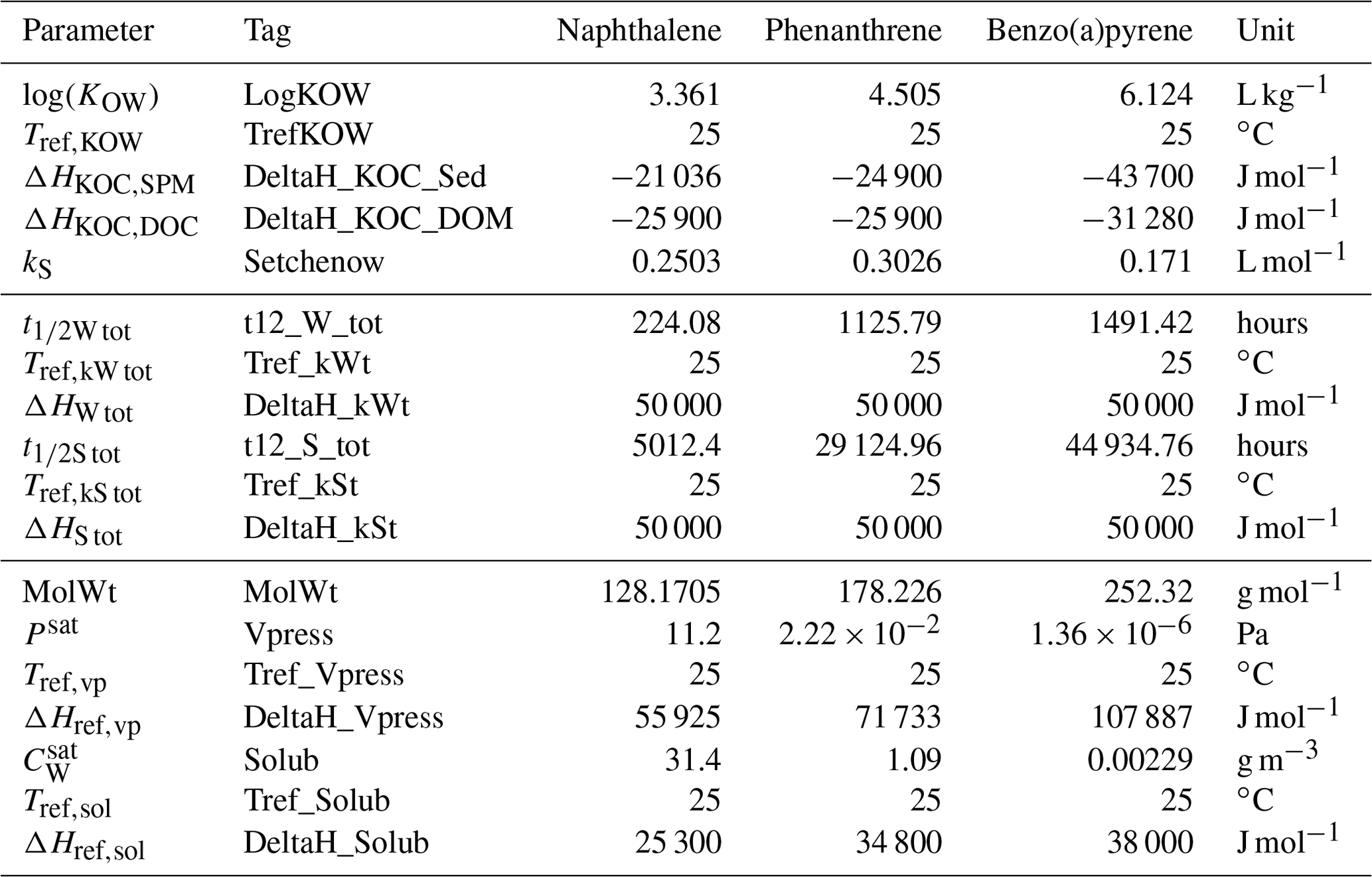
Table 2Chemical parameters utilized for modelling the sorption, degradation, and volatilization of three organic compounds.
In the Lagrangian framework utilized by the proposed model, concentrations are not calculated at each time step, and hence the equivalent effect is obtained by applying an exponential decay to the mass mi(t) of all dissolved elements i within the mixed layer, as expressed by .
As reported above, kvol can be estimated starting from MTCvol, whose reciprocal can be interpreted as the total resistance to the mass transfer through the two-film interface and therefore can be expressed as the sum of the resistances of each layer (Eq. 15):
Here, MTCa and MTCw (m s−1) are the air-side and water-side mass transfer coefficients, respectively, and Hcc is the dimensionless Henry law constant.
The diffusion rates of a chemical in these stagnant boundary layers can be related to the known diffusion rates of reference substances such as oxygen and water vapour (Schwarzenbach et al., 2016). Based on the boundary-layer theory (Deacon, 1977), the mass transfer coefficient for a target chemical can be obtained from these by applying a correction factor that depends on the ratios of the Schmidt numbers of the target and reference chemicals. The following relations proposed by McGillis et al. (2001) and (Johnson, 2010) and summarized by Schwarzenbach et al. (2016) are used in this work.
Here, MolWt (g mol−1) is the molecular weight of the target chemical, is the molecular weight of CO2 (44 g mol−1), is the molecular weight of water (18 g mol−1), U10 is the wind speed 10 m above the water surface (m s−1) and is the Schmidt number of water vapour in air (0.62). Then, Eqs. (16) and (17) are inserted into Eq. (15), where the dependencies on temperature and salinity are accounted for when the dimensionless Henry law volatility constant Hcc is calculated (Park and Clough, 2014) as
Here, R is the universal gas constant ( atm m3 mol−1 K−1), T is the temperature (K) and S is the salinity (PSU). The last term at the numerator is a dimensionless linear-correction factor for the effect of salinity, accounting for a factor of 1.4 for S=35 PSU compared to fresh water (Park and Clough, 2014; Schwarzenbach et al., 1993). Hpc is Henry's volatility constant (atm m3 mol−1), which is either specified by the user or estimated by
where Psat (atm) is the vapour pressure of the target chemical at the reference temperature, Csat (g m−3) is the solubility of the target chemical at the reference temperature, and are dimensionless temperature correction factors calculated with Eq. (10) for volatilization and solubilization reactions with the respective enthalpy changes ΔHvol and ΔHsol at the target temperature T.
3.1 Ship Traffic Emission Assessment Model (STEAM)
Emission fields from STEAM by Jalkanen et al. (2021) are used in this work. Modelled emissions from open-loop scrubbers in 2019 are utilized in the following examples. The method named seed_from_STEAM(…) is implemented in the ChemicalDrift class to allow seamless seeding of Lagrangian elements directly from the STEAM DataArray. Emission data are provided as a volume (m3) of discharged scrubber water at each spatio-temporal grid point. The conversion from volume to mass of chemicals is implemented within the class method, applying average emission factors (µg L−1) and confidence intervals reported in Lunde Hermansson et al. (2021) for open_loop and closed_loop scrubbers for a set of heavy metals and PAHs, selected with the arguments scrubber_type and chemical_compound, respectively. The total mass of chemicals for each STEAM data point is then distributed on a number of Lagrangian elements with a given mass and over a circular area defined by the arguments mass_element_ug (µg) and radius (m).
3.2 Chemical parameters for PAHs
A database of parameters for a set of organic compounds and heavy metals has been compiled under the scope of the EMERGE project, based on an extensive review of data available in the literature. Mean values from the database for a selection of PAHs are integrated into the ChemicalDrift class method init_chemical_compound, which allows one to configure the whole set of parameters by simply selecting the target chemical. Alternatively, each parameter can be specified singularly with the set_config method. Both procedures are shown in the example in Listing 1, while the data for the PAHs utilized in this work are reported in Table 2.
3.3 Metocean forcing from CMEMS and the System of HydrodYnamic Finite Element Modules (SHYFEM)
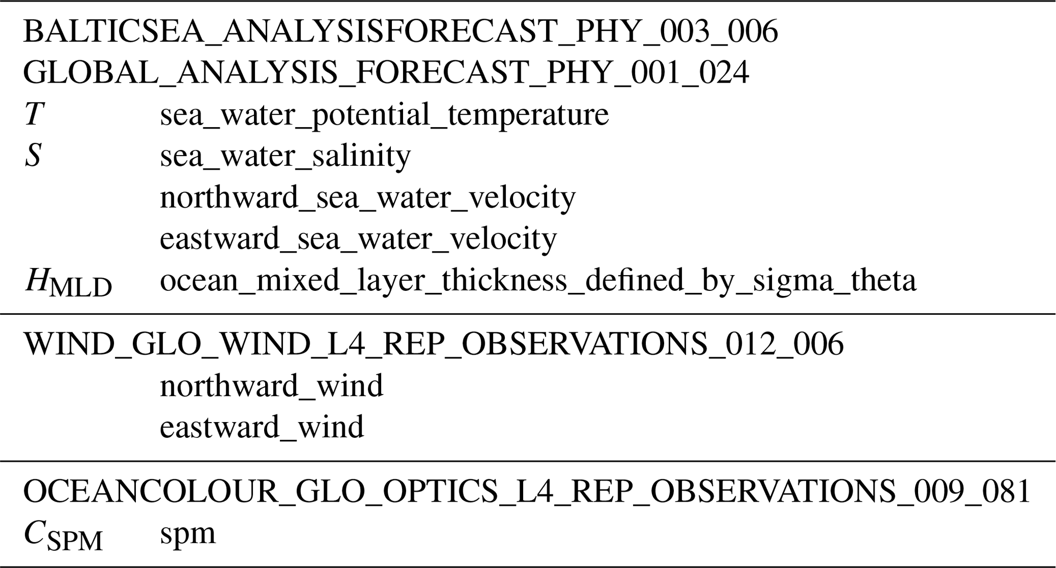
Meteorological and oceanographic forcing is obtained from different sources. Several CMEMS products are utilized in this work, providing water temperature, salinity, current horizontal velocities, mixed-layer depth, ocean surface winds, and SPM concentration, as summarized in Table 3.
High-resolution 3-D currents, water temperature and salinity forcing over the northern Adriatic Sea including the Venice Lagoon are provided by the application of the unstructured hydrodynamic SHYFEM model (Bellafiore et al., 2018). SHYFEM model integrations are performed on a spatial domain covering the whole of the Adriatic Sea and its main coastal lagoons (Marano-Grado, Venice, and the Po River delta). To adequately resolve the river–sea continuum, the unstructured grid also includes the lower part of the major rivers flowing into the Adriatic Sea. The numerical grid consists of approximately 110 000 triangular elements with a resolution that varies from 5 km in the open sea to a few hundred metres along the coast and tens of metres in the inner lagoon channels (Ferrarin et al., 2019).
The SHYFEM simulations are forced by atmospheric fields from the global ECMWF reanalysis ERA5 (Hersbach et al., 2020), sea boundary and initial conditions from the Mediterranean Forecast System reanalysis (Tonani et al., 2009) and observed or climatological water discharges at the main river mouths.
The ChemicalDrift functionalities are demonstrated through a few modelling examples described in the following. The presented simulations are not meant to provide conclusive quantitative results as some of the input parameters are uncertain and the model remains to be validated. The examples are run with OpenDrift 1.9.0 (e.g.) and may not be functional in the far future.
4.1 Organic pollutant discharge in Kattegat
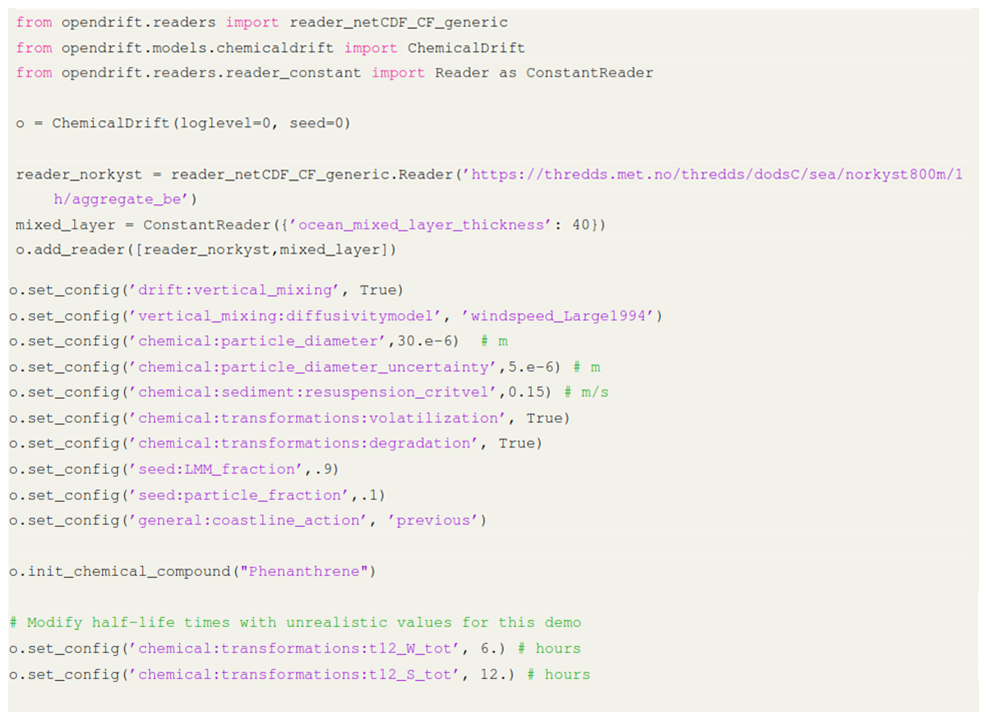
A simple example of a ChemicalDrift simulation is presented with a description of the running script. The example is also available in the gallery section on the OpenDrift reference page (opendrift.github.io), where it is continuously updated with live forcing data. The simulation models the fate of a mass of an organic pollutant (phenanthrene) released outside the northern coast of Denmark over a period of 2 d. Simulation set-up is done as shown in the listing below by loading the OpenDrift modules, defining a ChemicalDrift instance, adding the necessary readers for forcing data and configuring a set of parameters. In detail, metocean forcing data including surface winds, ocean currents, sea water temperature and salinity are provided by the Norkyst800 model, while mixed-layer depth is set to a constant value of 40 m. Vertical mixing is activated, and the model used for the diffusivity profile is selected. Released chemicals are assumed to be 90 % in the dissolved fraction, and 10 % are adsorbed to particles. Degradation rates for phenanthrene are overridden in order to produce a clear effect in this short demo, and half-life constants are set to 6 h in the water column and 12 h in the sediment layer.
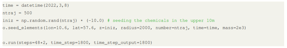
The model is configured at this stage. The next step is to seed the Lagrangian chemical elements and run the simulation. In this example, 500 chemical elements with a mass of 2000 µg are seeded within a radius of 2000 m around the selected position and within the upper 10 m of the water column.
Simulation results are illustrated in Fig. 2, showing how the chemical is partitioned between the dissolved, adsorbed-to-SPM and sediment compartments and advected in the northward direction. As expected, dissolved chemicals are mainly close to the surface and transported horizontally at higher velocities, while it can be seen that elements adsorbed to SPM travel for shorter distances at a higher depths. The distribution of mass between the three modelled compartments is shown in Fig. 3, where the exponential decay due to the combined effect of degradation and volatilization can also be observed. In detail, due to the short half-lives used in the simulation, more than 40 % of the initial mass was removed during the simulated period. Two clear strong resuspension events are illustrated after approximately 8 and 34 h, as shown by the rapid increase in the mass of chemicals associated with SPM at the expense of the sediment compartment followed by periods with a pre-dominant exchange in the opposite direction as elements representing suspended particles are sedimented again.

Figure 2Simulated transport and fate of a mass of phenanthrene released outside the northern coast of Denmark, showing horizontal advection (a, b, c) and vertical distribution in the water column and at the sea floor (d, e, f). The colour of the Lagrangian elements indicates the partitioning between dissolved, adsorbed to SPM, and sediments.
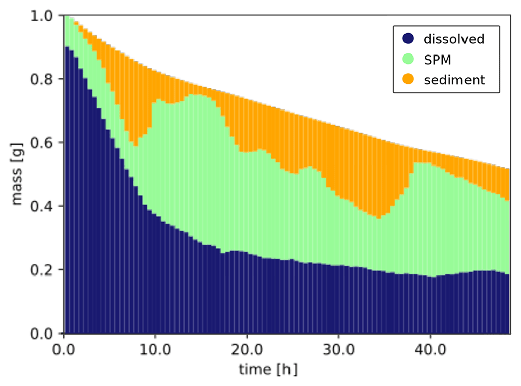
Figure 3Exponential decay and mass distribution across the dissolved, adsorbed-to-SPM, and sediment phases for phenanthrene.
4.2 Naphthalene and benzo(a)pyrene discharges from open-loop scrubbers
ChemicalDrift is demonstrated using input data from the STEAM model to simulate emissions of selected PAHs (i.e. naphthalene and benzo(a)pyrene) from open-loop scrubbers. The simulated region includes emissions for January 2019 in the area between 8 and 15∘ E and between 53 and 60∘ N. The simulation also covers an additional period of 2 months after the emission of the target chemicals ended, showing how the different chemical properties (Table 2) strongly influence their environmental fate. Results are illustrated in Figs. 4 and 5. In both figures we see that naphthalene is predominantly in the dissolved phase, while benzo(a)pyrene, which has a 3 orders of magnitude larger KOW, is mostly adsorbed to particles. Initial discharges along ship lanes are observed in Fig. 4a and d. In the figure the diameter of each Lagrangian element is reduced as its associated mass decreases, indicating the target chemical's removal by degradation and volatilization. This is clearly observed for naphthalene (top right), while benzo(a)pyrene (bottom right) is almost entirely preserved in the simulated period since it has much longer half-life values and is to a large degree adsorbed to particles and more rapidly deposited to the sediment layer, where its degradation is much slower. The same conclusions about the different behaviours of the two chemicals are also observed in Fig. 5, which illustrates the two chemicals' vertical profiles in the water column and sediments (top) and the time evolution and phase partitioning of the mass of the chemicals (bottom).
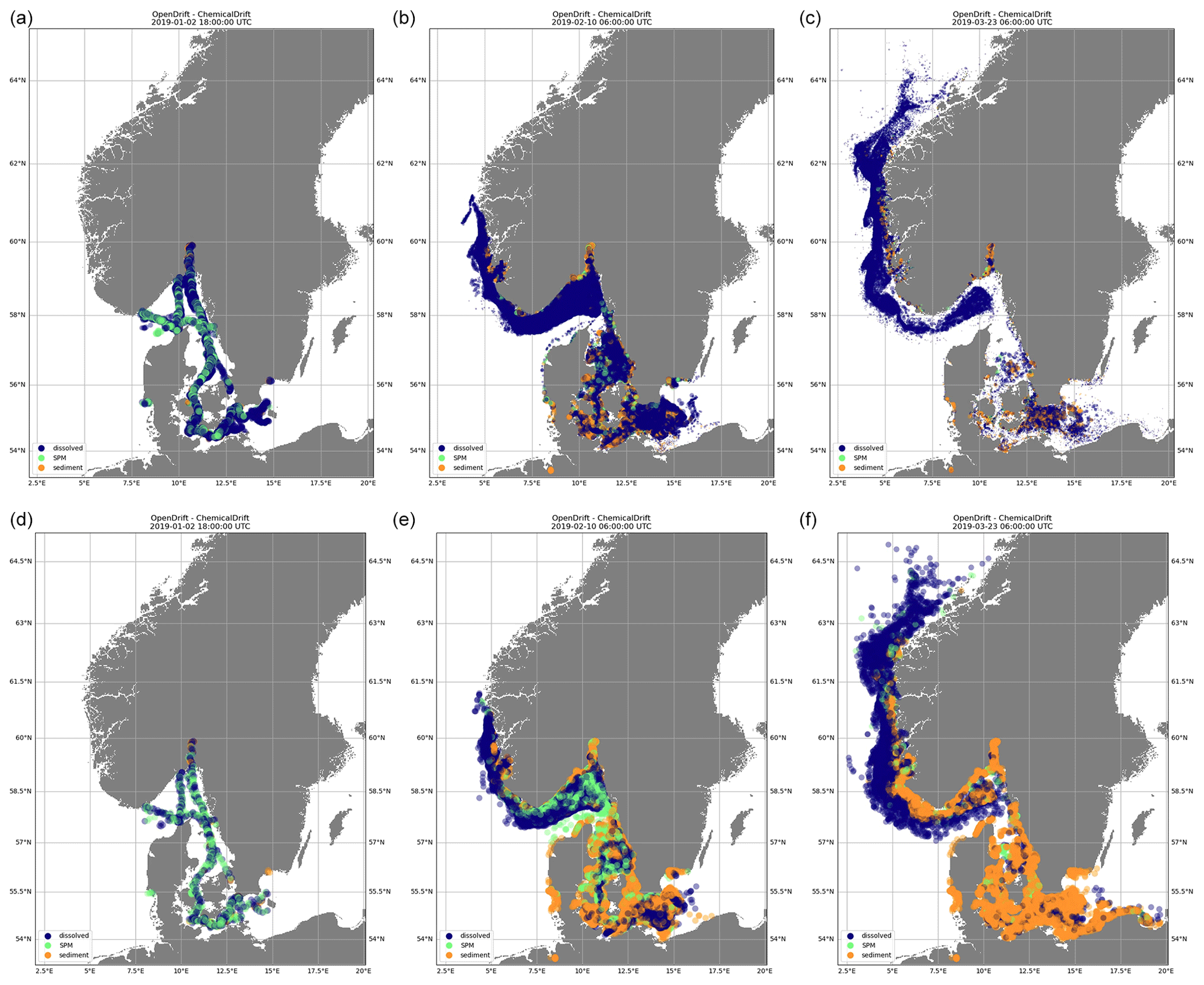
Figure 4Emissions of naphthalene (a, b, c) and benzo(a)pyrene (d, e, f) from open-loop scrubbers derived from the STEAM model for January 2019 in the sea region around Denmark. Element diameter is directly proportional to the associated mass. Transport and fate are calculated by ChemicalDrift over a 3-month period. Naphthalene is predominantly in the dissolved phase and more easily degraded and volatilized. Benzo(a)pyrene is mostly adsorbed to suspended particles and deposited to the sediment layer.

Figure 5Emissions of naphthalene (a, c) and benzo(a)pyrene (b, d) from open-loop scrubbers derived from the STEAM model for January 2019 in the sea region around Denmark. Northward view of the distribution of chemicals in the water column and sea floor after 3 months (a, b) and evolution of the mass of chemicals in each model phase (c, d).
4.3 Multiple emission sources in the Adriatic Sea
Modelling of emissions from multiple sources is demonstrated. The target chemical considered is benzo(a)pyrene, and emissions include discharges estimated in August 2019 from open-loop scrubber data derived from STEAM and discharges from 49 rivers obtained from water-quality monitoring data and river loads.
Snapshots of the simulation are shown in Fig. 6, where colours are used to identify model compartments (panels a and b) and emission sources (i.e. ships or rivers, panels c and d). Emissions from scrubbers are to a large degree confined to the proximity of shipping lanes even at the end of the simulated period, and this is explained by also considering that benzo(a)pyrene has a high KOW (Table 2) and is strongly associated with the solid fraction which is rapidly deposited to the sediment layer in proximity to the ship tracks. For the same reason, emissions from the rivers are mostly located along the shallow coastal regions and slowly transported southwards by the cyclonic Adriatic gyres.
Simulation results are further illustrated in Fig. 7, where the mass of target chemicals and the corresponding mass removed by degradation and volatilization are plotted versus time. The total emitted mass of chemicals in August 2019 is 17 500 g, and only about 500 g is removed by the end of September 2019. Degradation is dominant (470 g) compared to volatilization (30 g), which is also explained by the strong affinity of benzo(a)pyrene with the solid fraction, which does not volatilize. Most of the degraded mass is removed in the dissolved phase, even if most of the chemicals are associated with the sediment layer, which is explained since is approximately 30 times shorter than (Table 2).
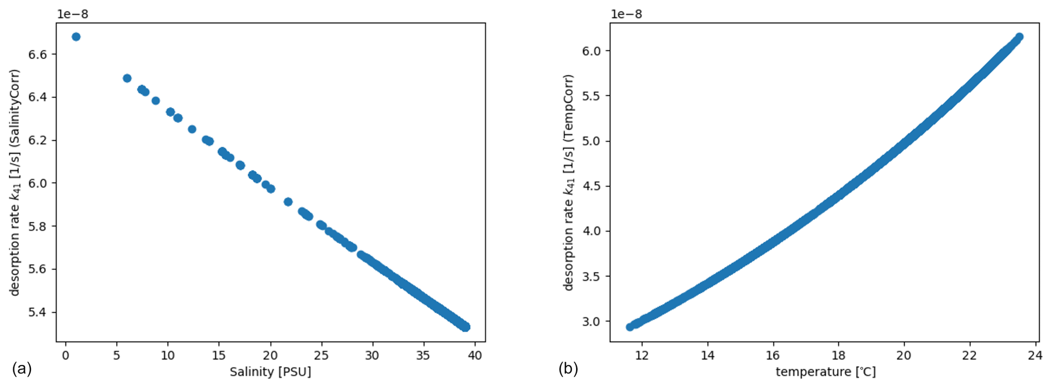
The example is also utilized to illustrate the dependency on temperature and salinity of the solid–water partition coefficient which is calculated according to Eqs. (8)–(10). This is reflected e.g. in the desorption rate from the sediment to the dissolved phase, k41 (Eq. 2), as shown in Fig. 8.
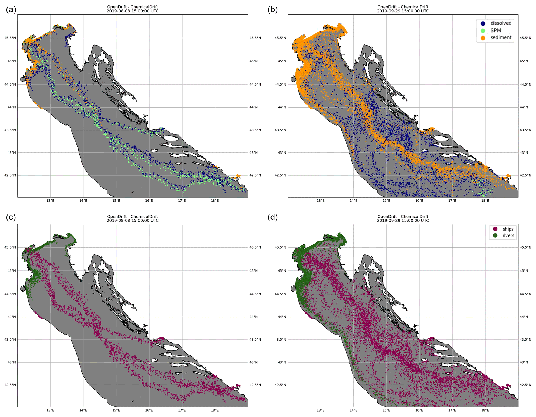
Figure 6Emissions of benzo(a)pyrene from both open-loop scrubbers and rivers in the northern Adriatic Sea for August 2019, simulated in ChemicalDrift over a 2-month period, showing how the use of Lagrangian modelling allows for seamless separation of the different sources. Two time steps are shown, 8 August 2019 (a, c) and 29 September 2019 (b, d). The colours indicate the phase partitioning (a, b) and the pollutant source (c, d).
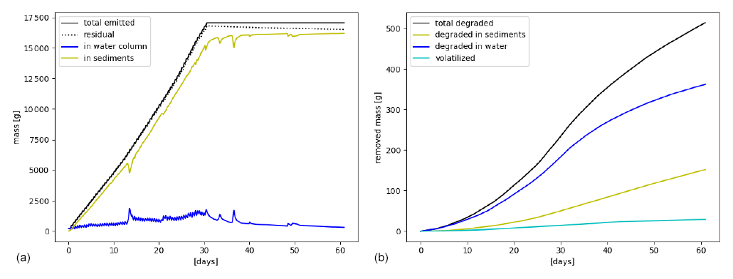
Figure 7Emissions of benzo(a)pyrene from open-loop scrubbers and rivers in the northern Adriatic Sea. Total emitted mass (a) and removed mass by degradation and volatilization (b). Mass in water column refers to all phases in the water column, including the dissolved and SPM phases.
4.4 Modelling of open-loop scrubber emissions in European seas
ChemicalDrift is applied to open-loop scrubber emissions for the entire European region from January to March 2019. The target chemical is phenanthrene, and fate and transport modelling are calculated until December 2019. This example is utilized to demonstrate the method write_netcdf_chemical_density_map(…), which is implemented in ChemicalDrift by adapting the corresponding method in the Radionuclides module. The method calculates gridded concentrations of the target chemical and exports these to a netCDF file. Gridding is applied as a post-processing step at the end of the simulation, providing average concentrations (10×10 km, user-definable) of the target chemical over the whole domain for each of the modelled phases. Estimated environmental concentrations are shown in Fig. 9. The time step for the averaging in each grid box is also user-definable. For the modelled phases in the water column, e.g. the dissolved and adsorbed-to-SPM phases, it is possible to define vertical grid size or to consider as in this case the whole column from the surface to the sea floor. Concentrations are saved to netCDF files. Results for the sediment phase are plotted (µg kg−1), where the mass of the chemical is the mass of Lagrangian elements deposited on the sediment layer in each grid box, and the total solid mass is calculated from user-definable sediment density and active-layer depth and porosity.
We see that only a few ships with scrubbers were operating in the Mediterranean in 2019, since it was before global sulfur cap regulation. Dissolved chemicals are more diffused, while chemicals attached to particles sink and have smaller lateral diffusion, and hence ship routes are more easily observed.
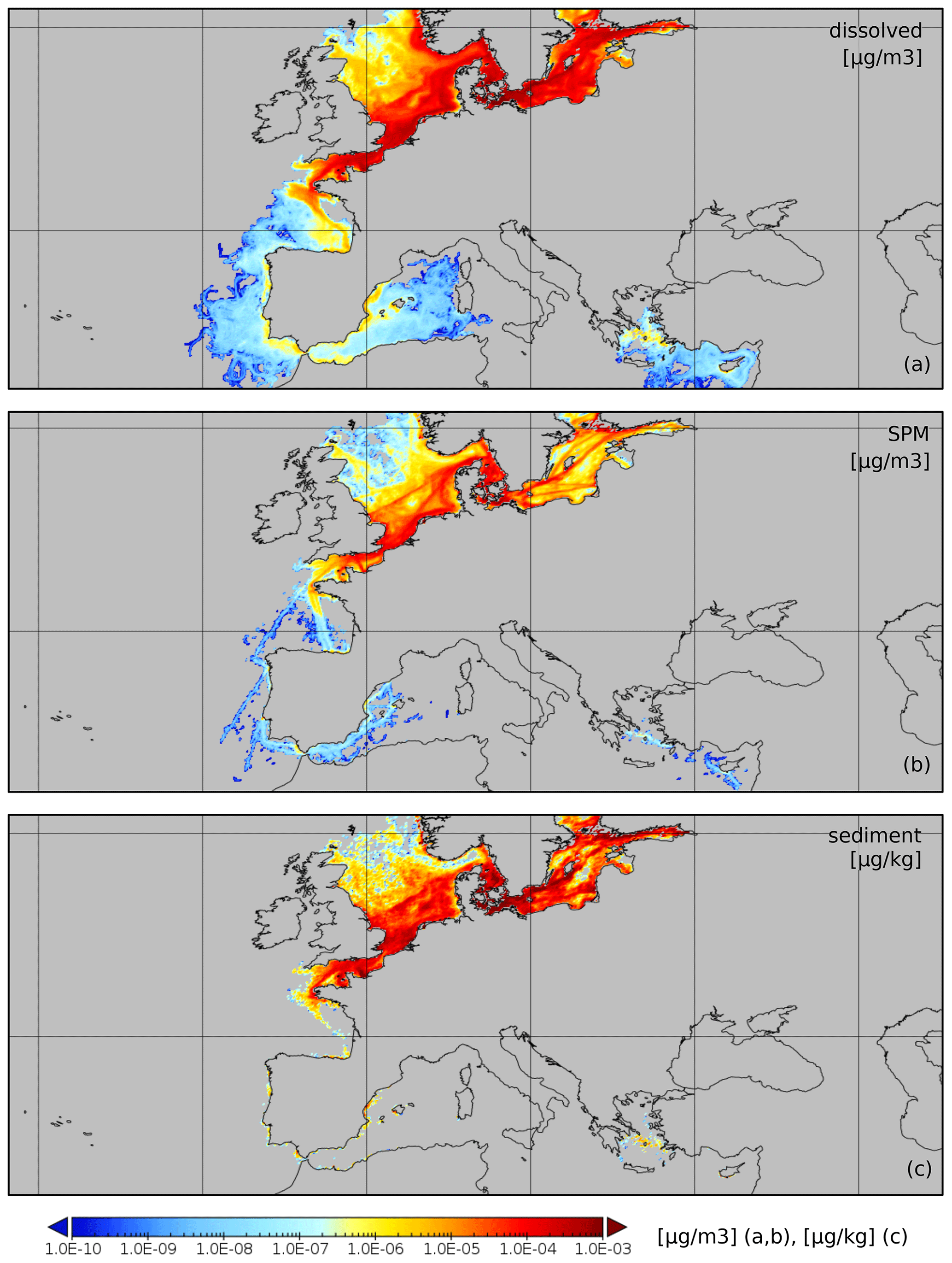
Figure 9Mean concentrations of phenanthrene emitted from open-loop scrubbers (January–March 2019). Concentrations are calculated separately for the dissolved (a), adsorbed to SPM (b), and sediments fractions (c).
ChemicalDrift, a new Lagrangian model for transport and fate of chemicals in the aquatic environment, has been presented. The model is implemented as a new module and is fully integrated within the open-source framework OpenDrift in order to combine the newly implemented chemical processes with the framework's advanced hydrodynamical capabilities and to provide a flexible interface with most of the available metocean input data sources.
The modelled chemical processes include a dynamic partitioning between the different phases that pollutants can be associated with in the aquatic environment, chemical removal by degradation and volatilization, and sedimentation and resuspension of chemicals associated with suspended particles. Target chemicals are modelled as Lagrangian elements that are transported and exposed to changing environmental conditions, e.g. temperature and salinity. The dependencies of chemical processes on temperature and salinity changes are formulated and implemented.
The focus of the presented work has been on modelling organic pollutants in the marine and coastal regions. The model functionalities are demonstrated through a sequence of simulation examples. The presented examples are only for demonstration purposes, providing insights into the combined effect of the modelled physical and chemical processes and presenting the potential of the proposed model. Accurate tuning of input parameters, sensitivity analysis, model validation and quantitative modelling results are deferred to future publications. Specifically, in the scope of the Horizion 2020 EMERGE project, ChemicalDrift is planned for use in calculating concentrations of different pollutants, including PAHs and heavy metals, both at the European regional scale and at a finer scale in the northern Adriatic Sea and in the Øresund strait. Additionally, the model can also be applied to other case-study areas in the EMERGE project, namely the Piraeus port-case study and the Aveiro Lagoon case study, where the Delft3D suite will be utilized independently by other project partners, allowing one to compare the results between the two models. Datasets with measured concentrations of organic pollutants in sediments obtained from monitoring programmes in the Baltic region and in the northern Adriatic are identified and available and can be used in the future to attempt validation of the model.
Additional functionalities are also planned for the future, including support for hydrolysis, photolysis and biodegradation as distinct sub-processes, support for non-ionizable organic compounds and a more advanced resuspension scheme which will include the contribution of wave-induced stress to resuspension.
High flexibility is demonstrated by the presented examples, utilizing a selection of different input sources and at different spatio-temporal scales: an interface to the STEAM model for shipping emissions, including support for open-loop and close-loop scrubbers, is implemented and demonstrated. The Lagrangian framework offers seamless tracking and separation of chemicals emitted from different sources such as emissions from shipping or from rivers. The modelled chemical processes depend on a relatively large set of parameters, including e.g. the solid–water partitioning coefficient, the Henry law coefficients and the overall degradation rates. A database of chemical parameters for a set of PAHs is integrated into ChemicalDrift, and values for the three PAHs are presented.
The ChemicalDrift model is freely available at the OpenDrift github repository at https://github.com/OpenDrift/opendrift/blob/master/opendrift/models/chemicaldrift.py (last access: 28 April 2023) under the terms of the GNU General Public License as published by the Free Software Foundation, version 2. The exact version used for the simulations presented in this work is integrated into OpenDrift 1.9.0 and is archived at https://doi.org/10.5281/zenodo.7429158 (Aghito, 2022a). The example presented in Sect. 4.1 is described with the complete running script and is available at the OpenDrift reference page (https://opendrift.github.io, last access: 28 April 2023) under the gallery section including the required input data. The following examples require datasets available at the Copernicus Marine Service, gridded bathymetry data that are available at GEBCO, and emissions from STEAM and ocean forcing from SHYFEM. The scripts to generate the examples including input data are archived at https://doi.org/10.5281/zenodo.7249446 (Aghito, 2022b).
MA designed and developed the model, performed and analysed the simulations and wrote the manuscript draft. LC contributed with model design, compiled the input data and wrote the introduction section. CF provided the SHYFEM model results and wrote the description of the model in Sect. 3.3. KFD supported the development. MA, LC, LRH, ØB, KFD, CF and AM reviewed and edited the manuscript.
The contact author has declared that none of the authors has any competing interests.
This work reflects only the authors’ view, and the European Climate, Infrastructure and Environment Executive Agency is not responsible for any use that may be made of the information it contains.
Publisher's note: Copernicus Publications remains neutral with regard to jurisdictional claims in published maps and institutional affiliations.
Mattia Boscherini (Ca'Foscari University of Venice) and Isabel Hanstein (University of Heidelberg) are kindly thanked for the valuable support in the compilation of the PAH chemical property database. The authors are grateful to Jukka-Pekka Jalkanen (Finnish Meteorological Institute) for providing the results of the STEAM model used in this work.
This project has received funding from the European Union’s Horizon 2020 research and innovation programme under grant agreement no. 874990 (EMERGE project). This research has also been supported by the Research Council of Norway (STIM-EU, project no. 334015).
This paper was edited by Andrew Yool and reviewed by two anonymous referees.
Ådlandsvik, B.: VertEgg – a toolbox for simulation of vertical distributions of fish eggs, version 1.0, Institute of Marine Research, Bergen, 66 pp., 2000. a
Aghito, M.: ChemicalDrift 1.0: code (1.0), Zenodo [code], https://doi.org/10.5281/zenodo.7429159, 2022a. a
Aghito, M.: ChemicalDrift 1.0: code and data (1.0), Zenodo [code and data set], https://doi.org/10.5281/zenodo.7249447, 2022b. a
Azarpira, M., Zarrati, A. R., and Farrokhzad, P.: Comparison between the Lagrangian and Eulerian Approach in Simulation of Free Surface Air-Core Vortices, Water, 13, 726, https://doi.org/10.3390/w13050726, 2021. a
Becker, A., Wotawa, G., De Geer, L.-E., Seibert, P., Draxler, R. R., Sloan, C., D’Amours, R., Hort, M., Glaab, H., Heinrich, P., Grillon, Y., Shershakov, V., Katayama, K., Zhang, Y., Stewart, P., Hirtl, M., Jean, M., and Chen, P.: Global backtracking of anthropogenic radionuclides by means of a receptor oriented ensemble dispersion modelling system in support of Nuclear-Test-Ban Treaty verification, Atmos. Environ., 41, 4520–4534, https://doi.org/10.1016/j.atmosenv.2006.12.048, 2007. a
Bellafiore, D., Mc Kiver, W., Ferrarin, C., and Umgiesser, G.: The importance of modeling nonhydrostatic processes for dense water reproduction in the southern Adriatic Sea, Ocean Model., 125, 22–28, https://doi.org/10.1016/j.ocemod.2018.03.001, 2018. a
Brekke, C., Espeseth, M. M., Dagestad, K.-F., Röhrs, J., Hole, L. R., and Reigber, A.: Integrated Analysis of Multisensor Datasets and Oil Drift Simulations – A Free-Floating Oil Experiment in the Open Ocean, J. Geophys. Res.-Oceans, 126, e2020JC016499, https://doi.org/10.1029/2020JC016499, 2021. a
Calgaro, L., Badetti, E., Bonetto, A., Contessi, S., Pellay, R., Ferrari, G., Artioli, G., and Marcomini, A.: Consecutive thermal and wet conditioning treatments of sedimentary stabilized cementitious materials from HPSS® technology: Effects on leaching and microstructure, J. Environ. Manage., 250, 109503, https://doi.org/10.1016/j.jenvman.2019.109503, 2019. a
Calgaro, L., Contessi, S., Bonetto, A., Badetti, E., Ferrari, G., Artioli, G., and Marcomini, A.: Calcium aluminate cement as an alternative to ordinary Portland cement for the remediation of heavy metals contaminated soil: mechanisms and performance, J. Soil. Sediment., 21, 1755–1768, https://doi.org/10.1007/s11368-020-02859-x, 2021. a
Chang, Y.-T., Park, H. K., Lee, S., and Kim, E.: Have Emission Control Areas (ECAs) harmed port efficiency in Europe?, Transport. Res. D, 58, 39–53, https://doi.org/10.1016/j.trd.2017.10.018, 2018. a
Dagestad, K.-F., Röhrs, J., Breivik, Ø., and Ådlandsvik, B.: OpenDrift v1.0: a generic framework for trajectory modelling, Geosci. Model Dev., 11, 1405–1420, https://doi.org/10.5194/gmd-11-1405-2018, 2018. a, b, c
D'Amours, R., Malo, A., Servranckx, R., Bensimon, D., Trudel, S., and Gauthier-Bilodeau, J.-P.: Application of the atmospheric Lagrangian particle dispersion model MLDP0 to the 2008 eruptions of Okmok and Kasatochi volcanoes, J. Geophys. Res.-Atmos., 115, D00L11, https://doi.org/10.1029/2009JD013602, 2010. a
Danovaro, R. and Boero, F.: Italian Seas, in: World Seas: an Environmental Evaluation, Elsevier, 283–306, https://doi.org/10.1016/B978-0-12-805068-2.00060-7, 2019. a
Deacon, E. L.: Gas transfer to and across an air-water interface, Tellus, 29, 363–374, https://doi.org/10.1111/j.2153-3490.1977.tb00746.x, 1977. a
Deltares: Delft3D WAVE User manual, Delft, https://content.oss.deltares.nl/delft3d4/D-Water_Quality_User_Manual.pdf, (last access: 28 April 2023), 2023. a
Draxler, R., Arnold, D., Chino, M., Galmarini, S., Hort, M., Jones, A., Leadbetter, S., Malo, A., Maurer, C., Rolph, G., Saito, K., Servranckx, R., Shimbori, T., Solazzo, E., and Wotawa, G.: World Meteorological Organization's model simulations of the radionuclide dispersion and deposition from the Fukushima Daiichi nuclear power plant accident, J. Environ. Radioactiv., 139, 172–184, https://doi.org/10.1016/j.jenvrad.2013.09.014, 2015. a
Fantke, P.: USEtox (R) 2.0 Documentation (Version 1.1), https://doi.org/10.11581/DTU:00000011, 2018. a
Ferrarin, C., Davolio, S., Bellafiore, D., Ghezzo, M., Maicu, F., Drofa, O., Umgiesser, G., Bajo, M., De Pascalis, F., Malguzzi, P., Zaggia, L., Lorenzetti, G., Manfè, G., and Mc Kiver, W.: Cross-scale operational oceanography in the Adriatic Sea, J. Oper. Oceanogr., 12, 86–103, https://doi.org/10.1080/1755876X.2019.1576275, 2019. a
Fofonoff, N. and Millard Jr, R.: Algorithms for the computation of fundamental properties of seawater, UNESCO Technical Papers in Marine Sciences, 44, https://doi.org/10.25607/OBP-1450, 1983. a
Galí, M., Falls, M., Claustre, H., Aumont, O., and Bernardello, R.: Bridging the gaps between particulate backscattering measurements and modeled particulate organic carbon in the ocean, Biogeosciences, 19, 1245–1275, https://doi.org/10.5194/bg-19-1245-2022, 2022. a
Hersbach, H., Bell, B., Berrisford, P., Hirahara, S., Horànyi, A., Munoz-Sabater, J., Nicolas, J., Peubey, C., Radu, R., Schepers, D., Simmons, A., Soci, C., Abdalla, S., Abellan, X., Balsamo, G., Bechtold, P., Biavati, G., Bidlot, J., Bonavita, M., De Chiara, G., Dahlgren, P., Dee, D., Diamantakis, M., Dragani, R., Flemming, J., Forbes, R., Fuentes, M., Geer, A., Haimberger, L., Healy, S., Hogan, R. J., Hólm, E., Janisková, M., Keeley, S., Laloyaux, P., Lopez, P., Lupu, C., Radnoti, G., de Rosnay, P., Rozum, I., Vamborg, F., Villaume, S., and Thépaut, J.-N.: The ERA5 global reanalysis, Q. J. Roy. Meteor. Soc., 146, 1999–2049, https://doi.org/10.1002/qj.3803, 2020. a
Hirdman, D., Sodemann, H., Eckhardt, S., Burkhart, J. F., Jefferson, A., Mefford, T., Quinn, P. K., Sharma, S., Ström, J., and Stohl, A.: Source identification of short-lived air pollutants in the Arctic using statistical analysis of measurement data and particle dispersion model output, Atmos. Chem. Phys., 10, 669–693, https://doi.org/10.5194/acp-10-669-2010, 2010. a
Hole, L. R., de Aguiar, V., Dagestad, K.-F., Kourafalou, V. H., Androulidakis, Y., Kang, H., Le Hénaff, M., and Calzada, A.: Long term simulations of potential oil spills around Cuba, Mar. Pollut. Bull., 167, 112285, https://doi.org/10.1016/j.marpolbul.2021.112285, 2021. a
Honti, M., Hahn, S., Hennecke, D., Junker, T., Shrestha, P., and Fenner, K.: Bridging across OECD 308 and 309 Data in Search of a Robust Biotransformation Indicator, Environ. Sci. Technol., 50, 6865–6872, https://doi.org/10.1021/acs.est.6b01097, 2016. a
Jalkanen, J.-P., Johansson, L., Wilewska-Bien, M., Granhag, L., Ytreberg, E., Eriksson, K. M., Yngsell, D., Hassellöv, I.-M., Magnusson, K., Raudsepp, U., Maljutenko, I., Winnes, H., and Moldanova, J.: Modelling of discharges from Baltic Sea shipping, Ocean Sci., 17, 699–728, https://doi.org/10.5194/os-17-699-2021, 2021. a
Johnson, M. T.: A numerical scheme to calculate temperature and salinity dependent air-water transfer velocities for any gas, Ocean Sci., 6, 913–932, https://doi.org/10.5194/os-6-913-2010, 2010. a
Karickhoff, S. W. and Morris, K. R.: Sorption dynamics of hydrophobic pollutants in sediment suspensions, Environ. Toxicol. Chem., 4, 469–479, https://doi.org/10.1002/etc.5620040407, 1985. a, b
Kettelarij, J., Ragas, A., and Oldenkamp, R.: ePiE exposure to Pharmaceuticals in the Environment ePiE technical model description, Tech. rep., https://i-pie.org/wp-content/uploads/2019/12/ePiE_Technical_Manual-Final_Version_20191202.pdf (last access: 28 April 2023), 2019. a, b, c, d
Kobayashi, T., Otosaka, S., Togawa, O., and Hayashi, K.: Development of a Non-conservative Radionuclides Dispersion Model in the Ocean and its Application to Surface Cesium-137 Dispersion in the Irish Sea, J. Nucl. Sci. Tech., 44, 238–247, https://doi.org/10.1080/18811248.2007.9711278, 2007. a
Lee, H.-J., Kim, S.-W., Brioude, J., Cooper, O. R., Frost, G. J., Kim, C.-H., Park, R. J., Trainer, M., and Woo, J.-H.: Transport of NOx in East Asia identified by satellite and in situ measurements and Lagrangian particle dispersion model simulations, J. Geophys. Res.-Atmos., 119, 2574–2596, https://doi.org/10.1002/2013JD021185, 2014. a
Lunde Hermansson, A., Hassellöv, I.-M., Moldanová, J., and Ytreberg, E.: Comparing emissions of polyaromatic hydrocarbons and metals from marine fuels and scrubbers, Transport. Res. D, 97, 102912, https://doi.org/10.1016/j.trd.2021.102912, 2021. a, b
McGillis, W. R., Edson, J. B., Hare, J. E., and Fairall, C. W.: Direct covariance air-sea CO2 fluxes, J. Geophys. Res.-Oceans, 106, 16729–16745, https://doi.org/10.1029/2000JC000506, 2001. a
Myksvoll, M. S., Jung, K.-M., Albretsen, J., and Sundby, S.: Modelling dispersal of eggs and quantifying connectivity among Norwegian coastal cod subpopulations, ICES J. Mar. Sci., 71, 957–969, https://doi.org/10.1093/icesjms/fst022, 2013. a
Naidu, R., Biswas, B., Willett, I. R., Cribb, J., Kumar Singh, B., Paul Nathanail, C., Coulon, F., Semple, K. T., Jones, K. C., Barclay, A., and Aitken, R. J.: Chemical pollution: A growing peril and potential catastrophic risk to humanity, Environ. Int., 156, 106616, https://doi.org/10.1016/j.envint.2021.106616, 2021. a
Onink, V., Jongedijk, C. E., Hoffman, M. J., van Sebille, E., and Laufkötter, C.: Global simulations of marine plastic transport show plastic trapping in coastal zones, Enviro. Res. Lett., 16, 064053, https://doi.org/10.1088/1748-9326/abecbd, 2021. a
Park, R. and Clough, J.: AQUATOX (Release 3.2) Volume 2: Technical Documentation, United States Environmental Protection Agency, https://www.epa.gov/sites/default/files/2018-09/documents/aquatox_tech_doc_3.2.pdf (last access: 28 April 2023), 2014. a, b, c, d, e, f, g
Parnis, J. M. and Mackay, D.: Multimedia Environmental Models, CRC Press, https://doi.org/10.1201/9780367809829, 2020. a
Paterson, S. and Mackay, D.: Interpreting chemical partitioning in soil–plant–air systems with a fugacity model, in: Plant Contamination: Modeling and Simulation of Organic ChemicalProcesses, edited by: Trapp, S. and McFarlane, J. C., Lewis, Boca Raton, FL, USA, 191–214, 1995. a
Periáñez, R.: A modelling study on 137Cs and 239,240Pu behaviour in the Alborán Sea, western Mediterranean, J. Environ. Radioactiv., 99, 694–715, https://doi.org/10.1016/J.JENVRAD.2007.09.011, 2008. a
Periáñez, R.: Modelling the environmental behaviour of pollutants in Algeciras Bay (south Spain), Mar. Pollut. Bull., 64, 221–232, https://doi.org/10.1016/j.marpolbul.2011.11.030, 2012. a
Periáñez, R. and Elliott, A. J.: A particle-tracking method for simulating the dispersion of non-conservative radionuclides in coastal waters, J. Environ. Radioactiv., 58, 13–33, https://doi.org/10.1016/S0265-931X(01)00028-5, 2002. a, b, c
Periáñez, R., Hierro, A., Bolívar, J. P., and Vaca, F.: The geochemical behavior of natural radionuclides in coastal waters: A modeling study for the Huelva estuary, J. Marine Syst., 126, 82–93, https://doi.org/10.1016/j.jmarsys.2012.08.001, 2013. a
Pirotta, E., Thomas, L., Costa, D. P., Hall, A. J., Harris, C. M., Harwood, J., Kraus, S. D., Miller, P. J., Moore, M. J., Photopoulou, T., Rolland, R. M., Schwacke, L., Simmons, S. E., Southall, B. L., and Tyack, P. L.: Understanding the combined effects of multiple stressors: A new perspective on a longstanding challenge, Sci. Total Environ., 821, 153322, https://doi.org/10.1016/j.scitotenv.2022.153322, 2022. a
Prata, A. J., Carn, S. A., Stohl, A., and Kerkmann, J.: Long range transport and fate of a stratospheric volcanic cloud from Soufrière Hills volcano, Montserrat, Atmos. Chem. Phys., 7, 5093–5103, https://doi.org/10.5194/acp-7-5093-2007, 2007. a
Röhrs, J., Dagestad, K.-F., Asbjørnsen, H., Nordam, T., Skancke, J., Jones, C. E., and Brekke, C.: The effect of vertical mixing on the horizontal drift of oil spills, Ocean Sci., 14, 1581–1601, https://doi.org/10.5194/os-14-1581-2018, 2018. a
Sardain, A., Sardain, E., and Leung, B.: Global forecasts of shipping traffic and biological invasions to 2050, Nat. Sustain., 2, 274–282, https://doi.org/10.1038/s41893-019-0245-y, 2019. a
Schwarzenbach, R., Gschwend, P., and Imboden, D.: Environmental organic chemistry, Wiley, New York, ISBN 978-0-471-83941-5, 1993. a
Schwarzenbach, R., Gschwend, P., and Imboden, D.: Environmental Organic Chemistry, John Wiley & Sons, ISBN 978-1-118-76723-8, 2016. a, b, c, d, e
Seiter, K., Hensen, C., Schröter, J., and Zabel, M.: Organic carbon content in surface sediments – Defining regional provinces, Deep-Sea Res. Pt. I, 51, 2001–2026, https://doi.org/10.1016/j.dsr.2004.06.014, 2004. a
Simonsen, M., Lind, O. C., Øyvind Saetra, Isachsen, P. E., Teien, H. C., Albretsen, J., and Salbu, B.: Coastal transport of river-discharged radionuclides: Impact of speciation and transformation processes in numerical model simulations, Sci. Total Environ., 669, 856–871, https://doi.org/10.1016/J.SCITOTENV.2019.01.434, 2019a. a, b, c, d, e
Simonsen, M., Teien, H. C., Lind, O. C., Øyvind Saetra, Albretsen, J., and Salbu, B.: Modeling key processes affecting Al speciation and transport in estuaries, Sci. Total Environ., 687, 1147–1163, https://doi.org/10.1016/J.SCITOTENV.2019.05.318, 2019b. a
Site, A. D.: Factors Affecting Sorption of Organic Compounds in Natural Sorbent/Water Systems and Sorption Coefficients for Selected Pollutants. A Review, J. Phys. Chem. Ref. Data, 30, 187–439, https://doi.org/10.1063/1.1347984, 2001. a
Stokes, G. G.: On the effect of the internal friction of fluids on the motion of pendulums, Transactions of the Cambridge Philosophical Society, 9, Part ii, 8–106, 1851. a
Sundby, S.: A one-dimensional model for the vertical distribution of pelagic fish eggs in the mixed layer, Deep-Sea Res. Pt. A, 30, 645–661, https://doi.org/10.1016/0198-0149(83)90042-0, 1983. a
Szymczycha, B., Zaborska, A., Bełdowski, J., Kuliński, K., Beszczyńska-Möller, A., Kȩdra, M., and Pempkowiak, J.: The Baltic Sea, in: World Seas: an Environmental Evaluation, Elsevier, 85–111, https://doi.org/10.1016/B978-0-12-805068-2.00005-X, 2019. a
Testa, D.: A note on the potential designation of the mediterranean sea as a sulphur emission control area, Mar. Policy, 121, 104145, https://doi.org/10.1016/j.marpol.2020.104145, 2020. a
Tonani, M., Pinardi, N., Fratianni, C., Pistoia, J., Dobricic, S., Pensieri, S., de Alfonso, M., and Nittis, K.: Mediterranean Forecasting System: forecast and analysis assessment through skill scores, Ocean Sci., 5, 649–660, https://doi.org/10.5194/os-5-649-2009, 2009. a
Turner, D. R., Hassellöv, I.-M., Ytreberg, E., and Rutgersson, A.: Shipping and the environment: Smokestack emissions, scrubbers and unregulated oceanic consequences, Elementa, 5, 45, https://doi.org/10.1525/elementa.167, 2017. a
Turner, D. R., Edman, M., Gallego-Urrea, J. A., Claremar, B., Hassellöv, I.-M., Omstedt, A., and Rutgersson, A.: The potential future contribution of shipping to acidification of the Baltic Sea, Ambio, 47, 368–378, https://doi.org/10.1007/s13280-017-0950-6, 2018. a
van Sebille, E., Griffies, S. M., Abernathey, R., Adams, T. P., Berloff, P., Biastoch, A., Blanke, B., Chassignet, E. P., Cheng, Y., Cotter, C. J., Deleersnijder, E., Döös, K., Drake, H. F., Drijfhout, S., Gary, S. F., Heemink, A. W., Kjellsson, J., Koszalka, I. M., Lange, M., Lique, C., MacGilchrist, G. A., Marsh, R., Mayorga Adame, C. G., McAdam, R., Nencioli, F., Paris, C. B., Piggott, M. D., Polton, J. A., Rühs, S., Shah, S. H., Thomas, M. D., Wang, J., Wolfram, P. J., Zanna, L., and Zika, J. D.: Lagrangian ocean analysis: Fundamentals and practices, Ocean Model., 121, 49–75, https://doi.org/10.1016/j.ocemod.2017.11.008, 2018. a
Vedachalam, S., Baquerizo, N., and Dalai, A. K.: Review on impacts of low sulfur regulations on marine fuels and compliance options, Fuel, 310, 122243, https://doi.org/10.1016/j.fuel.2021.122243, 2022. a
Zhang, Y., Eastham, S. D., Lau, A. K., Fung, J. C., and Selin, N. E.: Global air quality and health impacts of domestic and international shipping, Environ. Res. Lett., 16, 084055, https://doi.org/10.1088/1748-9326/ac146b, 2021. a