the Creative Commons Attribution 4.0 License.
the Creative Commons Attribution 4.0 License.
 | 05 May 2023
Daily INSOLation (DINSOL-v1.0): an intuitive tool for classrooms and specifying solar radiation boundary conditions
Emerson D. Oliveira
Climate modelling requires spending an extensive amount of time programming, which means reading, learning, testing, and evaluating source code. Fortunately, many climate models have been developed within the past decades, making it easier for climate studies to be conducted on a global scale. However, some climate models have millions of code lines, making the introduction of new parameterizations a laborious task that demands teamwork. While it is true that the high-complexity models perform realistic climate simulations, some researchers perform their studies using simplified climate models in the preliminary test phases. This realization motivated the development of Daily INSOLation (DINSOL-v1.0), a robust computer program to support the simplified climate models, performing solar radiation calculations while considering Milankovitch cycles and offering various simulation options for its users. DINSOL was intended to function as a program that supplies data (e.g. daily insolation, instantaneous solar radiation, orbital parameters of the Earth, and calendar dates), such as the Paleoclimate Modelling Intercomparison Project (PMIP). While preparing the boundary conditions of solar radiation for climate models, it was realized that the DINSOL model could also be a helpful tool for use in classrooms. Thus, it was decided that an intuitive graphical user interface would be required to cater to this educational purpose. The model was written in the Fortran 90 language, while its graphical user interface would be built using PyGTK, a Python application programming interface (API) based on GIMP ToolKit (GTK). Furthermore, the R language would also be used to generate a panel containing contour fields and sketches of the orbital parameters to support the graphical execution. The model evaluation made use of data from PMIP and other tools, and the data analysis was performed through statistical methods. Once all tests were concluded, an insignificant difference between the DINSOL-obtained results and the results obtained from other models validated the viability of DINSOL as a dependable tool.
- Article
(9131 KB) - Full-text XML
-
Supplement
(3131 KB) - BibTeX
- EndNote


In paleoclimatology, greenhouse gases (GHGs) and other climate features, such as air temperature, can be estimated using indirect methods (e.g. ice cores, speleothems, tree rings, lake and marine sediments, glacier fluctuations) (Klippel et al., 2020). Paleoclimatology also investigates the effect that changes in the orbit of the Earth has on the incoming solar radiation (ISR). GHGs are vital because they affect the net radiation by increasing or decreasing the heat trapped in the atmosphere. Therefore, fluctuations in ISR or GHGs affect the global energy balance, meaning that they are factors in global climate change (Menviel et al., 2019; Lhardy et al., 2021). Berger (2021) details how a century ago, Milutin Milankovitch proposed a revolutionary approach to explaining the quasi-periodic occurrence of ice ages from caloric season measurements. It was because of his contributions that he has been considered to be the father of paleoclimate modelling. Thus, the conceptual climate model developed and adopted by Milankovitch assumed that ISR changes happened due to cyclic oscillations of the Earth's orbital parameters (EOPs): obliquity, eccentricity, and precession of the equinox. From Puetz et al. (2016), the initial Milankovitch theory was treated with scepticism due to previous theories on what causes ice ages, theories relating to the ejection of volcanic dust content in the atmosphere, as well as the cyclic changes in the magnetic field of the Earth.
Berger (2021) states that the most important books published by Milankovitch are Théorie mathématique (1920) and Kanon der Erdbestrahlung (1941). In these books and other literature, Milankovitch used EOP data previously calculated, adopting Stockwell–Pilgrim values from the theoretical investigations on ISR and ice ages. In accordance with Crucifix et al. (2009), besides Milankovitch, other authors investigated the relationship between ice ages and ISR, the most distinguished being André Berger, who developed a practical method to calculate the EOPs from trigonometric series. He also adopts the caloric seasons to investigate the past climate as a function of the EOPs. In the 1970s, Berger published papers (e.g. Berger, 1976, 1977, 1978a, b) that consolidated the modern concepts of ISR modelling. Since then, novel solutions for Earth's orbit cycles have been developed (e.g. Laskar, 1988; Berger and Loutre, 1991; Laskar et al., 1993, 2004, 2011).
Presently, the Paleoclimate Modelling Intercomparison Project (PMIP) represents the best efforts of the scientific community in paleoclimate reconstructions. PMIP is in its fourth phase (PMIP4), with some studies ongoing and others already been published (e.g. Jungclaus et al., 2017; Otto-Bliesner et al., 2017; Kageyama et al., 2018; Menviel et al., 2019). For instance, according to Brierley et al. (2020), PMIP simulations suggest that during the mid-Holocene, the most pronounced and robust monsoonal changes occurred over northern Africa and the Indian subcontinent, where the simulated rain rate was 10 % greater than the pre-industrial era (1850 CE). Therefore, climate reconstructions are crucial to enhancing the hold on understanding of natural forcings. Moreover, the Coupled Model Intercomparison Project (CMIP) is capable of handling various scenarios, considering natural and anthropogenic forcings, and reducing the uncertainties in climate projections (Eyring et al., 2016). Further, the Intergovernmental Panel on Climate Change (IPCC) is responsible for announcing the CMIP scenarios through assessment reports, focusing mainly on providing readable summaries for policymakers (Fischer et al., 2020).
In recent years, useful tools to aid in calculating the EOPs and insolation were developed, tools like PALINSOL, an R package written by Michel Crucifix that adopts Berger (1978b), Berger and Loutre (1991), and Laskar et al. (2004) solutions. Another tool is the Earth Orbit v2.1, a MATLAB program created by Kostadinov and Gilb (2014) to calculate the EOPs according to the Berger (1978b) and Laskar et al. (2004) methodologies. PALINSOL and other similar Fortran programs written by André Berger are available to download by the Université Catholique de Louvain (UCLouvain) through the Earth and Life Institute web page (https://www.elic.ucl.ac.be/modx/index.php?id=83, last access: 21 January 2023).
Even though we have pre-existing programs to calculate the ISR following the Milankovitch cycle theory, they were developed to cater to different purposes and kinds of users. For instance, the PALINSOL package assumes that users already know how to program in the R language, which could be an obstacle for students at the beginner level. Thus, Earth Orbit v2.1 could be an alternative to get around the programming skill requirement as it can be executed using a user-friendly graphical user interface (GUI). Even still, it is expected that the Earth Orbit v2.1 users buy a MATLAB licence, which could be prohibitive to disadvantaged groups. Furthermore, none of these programs were idealized to be executed from only one command line or clique and, from that, prepare the boundary conditions of simplified climate models. Therefore, it would be helpful to have another software option that works similarly to the pre-existent tools, but, additionally, it should be free and not require any programming language skills to execute simple tasks, such as computing the daily insolation globally for a given year.
To achieve this goal, the Daily INSOLation (DINSOL-v1.0) program was developed, intended to be an intuitive and versatile tool ideal for paleoclimate simulations, such as those performed on PMIP, and still helpful for education purposes. From DINSOL, users can prepare solar radiation as a boundary condition for simplified climate models quickly and flexibly. Moreover, the DINSOL source code brings many comments, allowing advanced users to modify and adapt it more intuitively than other tools. For instance, introducing a new calendar option to compute the annual daily insolation for an exoplanet is a simple task. Still, a standard execution offers users various input choices to run their DINSOL simulations (e.g. year, solar constant, calendar, latitudinal and longitudinal number points). It also includes a GUI, with the GUI written in PyGTK, a Python program that adopts the GIMP ToolKit (GTK) library. Basically, the DINSOL source code is mostly a Fortran program because all its important processes (e.g. data reading, taking decisions, calculation, and writing results) were written using the Fortran 90 language. Besides PyGTK and Fortran 90, the model also contains some script templates written in the R language to assist its users in accessing computed solar radiation data. The program has a GNU GPL v3.0 licence, which allows users to modify, share, and improve it. For instance, DINSOL was adapted to prepare ISR data for an energy balance model used by Oliveira and Fernandez (2020).
Ultimately, the following sections describe the program source code, giving a detailed explanation of the astronomical equations, ISR and EOP parameterizations, and input and output data. The “Model evaluation: a short statistical analysis” section adopts PMIP and other data sources as a reference.
This section details the astronomical fundamentals required to understand the DINSOL source code. The variables, constants, and mathematical relations are explained in the subsequent subsections.
2.1 Main orbital elements and some formulas
The DINSOL model utilizes heliocentric coordinates, such as in Berger (1978b) and Berger et al. (2010), and the most important information on the Earth's orbit is shown in Fig. 1. From the first figure, we have some orbital elements and constants for present day:
where S0 is the solar constant, T is the tropical year, a is the semi-major axis, and e is the eccentricity of the Earth's elliptical orbit. The longitude of the perihelion, ϖ, is kept unchanged and is given from the vernal point (21 March) until the perihelion day, and the longitude of the perigee, ω, is ϖ added to 180∘. As shown in Fig. 1, the Earth's orbital revolution occurs anti-clockwise, while the equinox precession occurs clockwise.
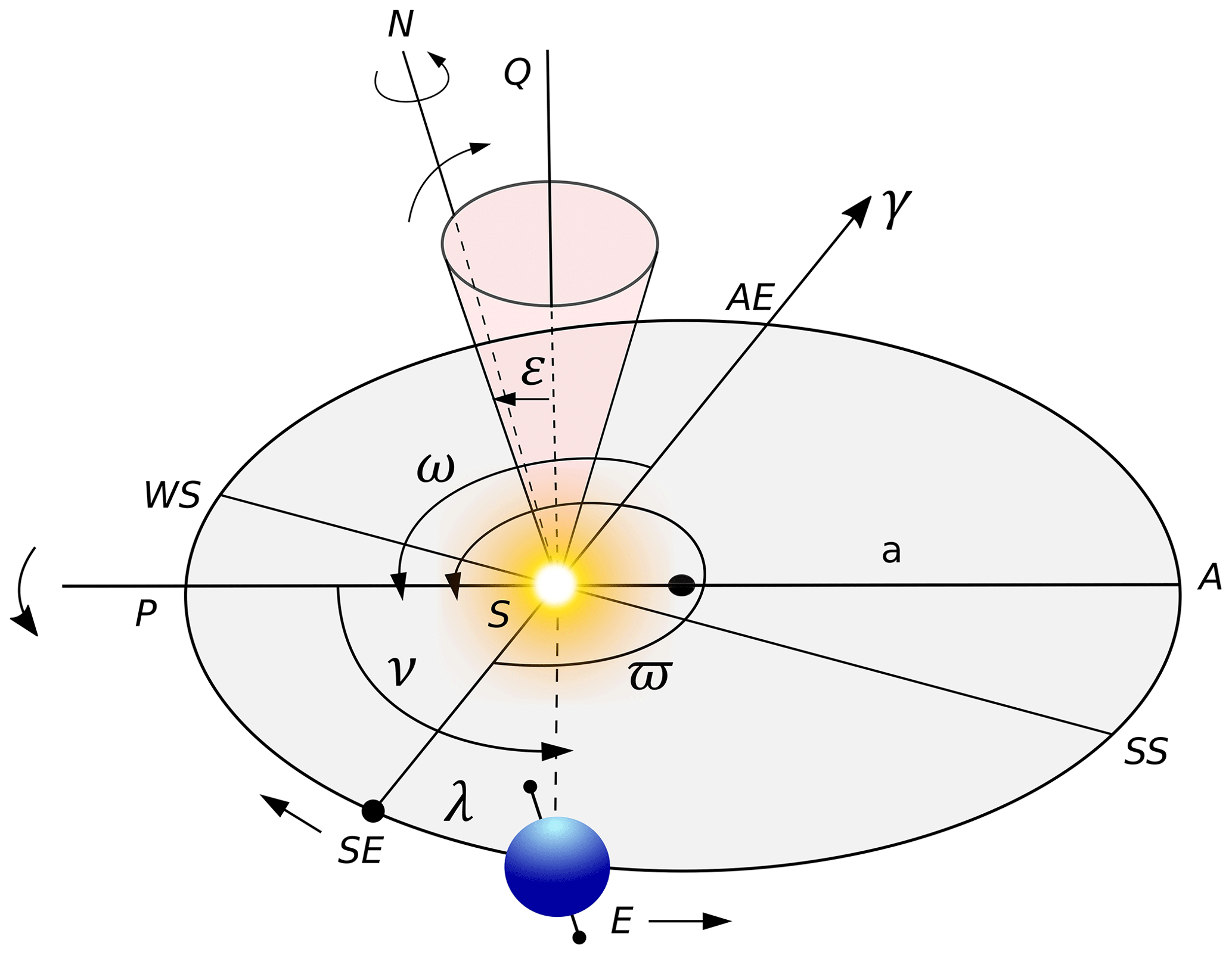
Figure 1Heliocentrical coordinate sketch based on Berger (1978b) and Berger et al. (2010). The orbital elements are denominated Earth, E; Sun, S; the semi-major axis of the Earth's orbit, a; perihelion, P; aphelion, A; vernal point, γ; spring equinox, SE; summer solstice, SS; autumn equinox, AE; winter solstice, WS; longitude of the perihelion, ϖ; longitude of the perigee, ω; true solar longitude, λ; true anomaly, ν; and obliquity, ε. The SQ is perpendicular to the ecliptic, and N is the north pole.
Regarding Fig. 1, the Earth's obliquity representing the equatorial plane, ε, is given by a cone perpendicular to the ecliptic plane; the Earth–Sun distance, r, is measured in units of the semi-major axis; and a is given by the ellipse equation:
where the relative Earth–Sun distance, ρ, provides values for an annual calendar, such as Fig. 2. The true anomaly, ν, is measured anti-clockwise from the perihelion and given by the equation , where λ represents the true solar longitude. Equation (1) is given in Beutler (2005, p. 127).
The DINSOL model implements the methodology from Berger (1978b), which solves λ in a few steps assuming that the start day is the vernal equinox (21 March), where λ=0. Thus, we first need to find the mean longitude λm; however, it is first necessary to calculate the λm0 using Eq. (2), where , and e is the eccentricity.
Finally, λ is calculated using Eq. (3), implementing a loop that solves λ over 1 year. However, for the first day (first iteration), the model requires the λm0 value obtained previously from Eq. (2), where we assume λm=λm0, to be employed. Hence, in the proceeding days, λm must be calculated from a simple increment equation given by the formula , where Nd represents the number of days within 1 year. In DINSOL, two annual calendars are available, a 365 and 360 d calendar.
Figure 2 represents the annual variation in Earth–Sun distance, ρ, for the present day. Furthermore, the data used to plot ρ were simulated using DINSOL, solving Eqs. (1) to (3). A calendar conversion was initialized with a starting date of 1 January instead of 21 March. The subsequent section contains all the details of the calendar conversions in the source code.
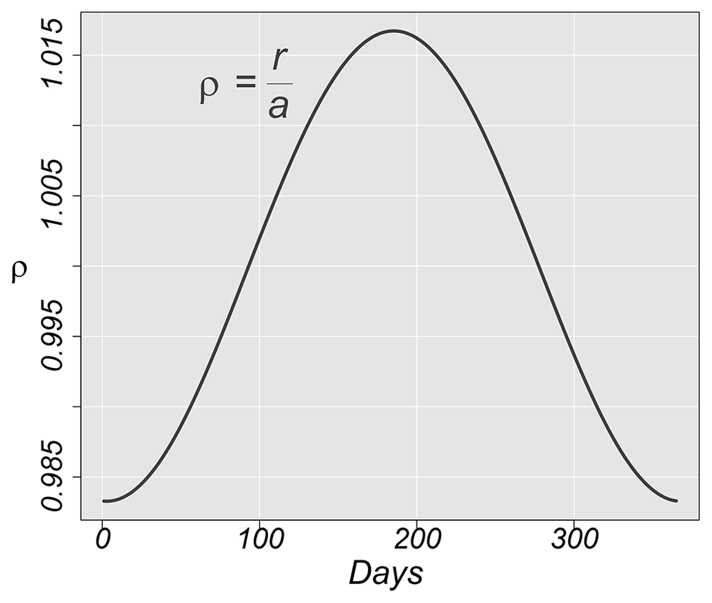
Figure 2Relative Earth–Sun distance, ρ, over 1 year in astronomical units (AU) for current days.
2.2 Defining the calendar dates
The daily insolation algorithm used in Berger (1978b) uses classical astronomical equations, where the year is initialized from spring equinoxes, like the solar Hijri calendar, also known as the Persian or Iranian calendar. The Persian calendar accurately calculates the length of a season due to the use of the true solar longitude, λ, which works on elliptical coordinates, like in Kepler's laws. Although Berger (1978b) assumed 21 March to be the fixed date for spring equinoxes, season dates oscillate over the years. For instance, in Borkowski (1996), in the second half of the 21st century, the spring equinoxes will occur on 19 and 20 March. An online program offered by NASA can accurately calculate the date of astronomical events using the Gregorian calendar (https://data.giss.nasa.gov/modelE/ar5plots/srvernal.html, last access: 21 January 2023). The Gregorian calendar is lunisolar and assumes the temporal definition of months and seasons, where the astronomical dates change slowly (Joussaume and Braconnot, 1997). For instance, considering λ, the assumption is that seasons stay 90∘ from one another along an elliptical orbit. Furthermore, a common challenge for paleoclimate simulations is the comparison of past and present climates, considering the differences between calendars.
From Bartlein and Shafer (2019a), the number of days in a month are not constant, which means that the first day of each month might occur in a different position relative to the current Gregorian calendar. For instance, in Joussaume and Braconnot (1997), during the Eemian periods, the month of January should have 34 d and start on 25 December relative to present days, which would be equivalent to 1 January. PMIP assumes the vernal equinox to be the time reference, keeping the current format of the Gregorian calendar for any period, which allows variations in season length, as well as changes in the aphelion and perihelion dates. From this method, the models can compare the results of paleoclimate simulations by using the same calendar structure, assuming a standard format. A typical PMIP experiment assumes a 365 d calendar, while intermediate-complexity climate models commonly work with a 360 d calendar.
The astronomical event dates (seasons, perigee, and apogee) are functions of the changes in two orbital parameters: eccentricity and precession of equinoxes. Furthermore, it must be noted that DINSOL supports a 365 and 360 d calendar. Consequently, it must be considered that the vernal equinox (21 March) always occurs on the 80th day of a 365 d calendar and on the 81st day of a 360 d calendar. Thus, a modified version of Eq. (2) must be implemented assuming a simple calendar conversion (solar to Gregorian calendar), where estimation of the perihelion and aphelion dates is made using Eq. (4).
where Pd represents the perihelion day in a solar calendar, and Pd can be converted for a day in the Gregorian calendar if Eq. (5) is used. Still, the vernal point (21 March) is called M21, which accepts the values 80 or 81 in concordance with the chosen calendar, Nd=365 or Nd=360, respectively.
After obtaining Pd for a day of the year in the Gregorian calendar, the aphelion day, Ad, can be determined by adopting Eq. (6):
The DINSOL model has a subroutine that converts the day of the year to its correspondent month and day. Moreover, beyond perihelion and aphelion dates, the start date of a season can be determined. A fixed date for the spring equinox (21 March) must be assumed, . Then, using the true solar longitude, λ, the summer, autumn, and winter start dates are known, at , , and , respectively. Hence, as is discussed in Sect. 2.1, λ must be solved using a loop to determine the iterations corresponding to λ equal to 90, 180, and 270∘. Furthermore, the DINSOL model uses a two-decimal precision, like in the PMIPII project. The calendar function evaluation is provided in Sect. 3.2.
2.3 Modelling the solar irradiance at the top of the atmosphere
In Fu (2006, p. 116), the incoming solar radiation (ISR) at the top of the atmosphere, S0, is estimated by the solar flux density (I0), which assumes an isotropic concentric emittance from the Sun. The total solar emittance, ES, must be constant, regardless of the size of the sphere area. The flux density adheres to the inverse square law, meaning that energy per area must diminish when the distance from the energy source increases, as shown in Fig. 3.

Figure 3Sketch of the solar flux density (I0) as a function of the distance to the Sun's core.
Therefore, ES can be estimated by multiplying the solar sphere area by the solar emission in a 1 m square, the emission being calculated using the Stefan–Boltzmann law, Eb=σT4, assuming the photosphere temperature and the solar radius to be T=6000 K and m, respectively (Hartmann, 2016, p. 29). The flux density at the Earth's orbital position, S0, can be estimated using a hypothetical solar sphere of radius m, the Earth–Sun distance. The solar constant is thus S0≈1366 W m−2.
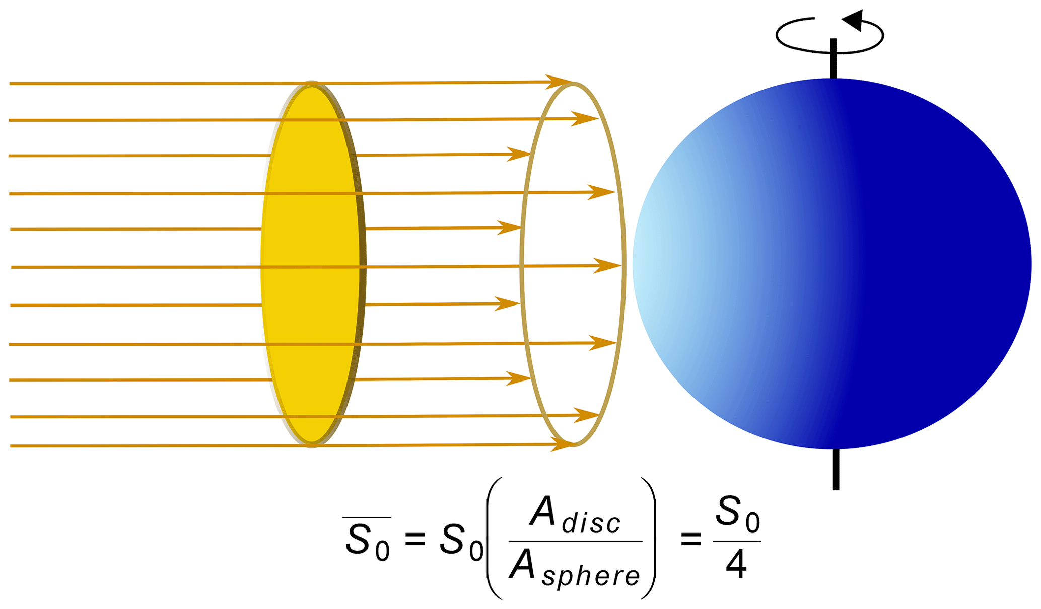
During simplified climate analysis, the global ISR average is , and because of the large Earth–Sun distance, the solar radiation is assumed to be a parallel and uniform beam (Hartmann, 2016, p. 31). Thus, to estimate , the total ISR inside of the disc area, the cross-section, must be divided by the Earth sphere area (Fig. 4), resulting in W m−2.
Although simplified climate approaches in zero-dimensional models are viable in classrooms, complex climate investigations require providing a realistic ISR. This way, the DINSOL model implements two different methods to calculate the ISR in the outer atmosphere. The first method is daily insolation (Q0), and the second is instantaneous solar radiation (QI). Thus, using this information, the methods can now be elaborated on.
2.3.1 Daily insolation
To calculate the ISR, aspects of ISR incidence on spherical surfaces must be considered (e.g. solar zenith angle, Z; hour angle, H; solar declination, δ; latitude, ϕ; and the relative Earth–Sun distance, ρ). Thus, In Liou (2002, p. 51), a realistic model of the daily insolation can be generated using Eq. (7):
where S0 is the solar constant, and represents the inverse square of the relative Earth–Sun distance, . The steps to calculate ρ are listed in Sect. 2.1. The solar zenith angle, Z, is obtained from the spherical law of cosines, shown in Eq. (8):
where h is the hour angle for a small time interval. To obtain the daily insolation, the total ISR at any latitude for a given day requires calculating daily ISR from sunrise (SR) to sunset (SS).
In Eq. (9) the constants for a given day are δ, ϕ, and . The hour angle and time are associated with the angular speed of Earth, Ω. Thus, a time differential substitution, dt, assuming , can be implemented. The result in Eq. (9) is a function of h:
where the hour angle from sunrise until solar noon is −H, and the hour angle from solar noon until sunset is +H. Then, solving the integral yields the following equation:
Therefore, assuming that the angular speed of Earth is , the equation for accumulated solar radiation in 1 d, that is, the daily insolation, can be found. However, the DINSOL model provides the daily average of the ISR, which requires the simplification of the equation by removing the total seconds per day. Finally, the equation implemented in the DINSOL source code is as follows:
Now, using Berger (1978b), to estimate Q0 following Eq. (12), it is necessary to calculate sin δ, cos δ, cos H, sin H, and H, which requires the implementation of these equations:
where λ is the true solar longitude, which has already been explained, and ε is the Earth obliquity; cos H demands the initialization of the following conditions.
Finally, these are the last steps:
Prior to the initialization of the instantaneous solar radiation method, the equation used to calculate the day length, in terms of number of hours of sunlight (N), is
2.3.2 Instantaneous solar radiation
The DINSOL model has a subroutine dedicated to calculating the instantaneous solar radiation, QI. This subroutine employs Eqs. (7) and (8). The main difference between QI and Q0 is that while Q0 stores a single value per day, QI can store several values per day (hours or minutes). Another key difference is that QI is calculated globally, while Q0 simulates only the latitudinal effect. Below is Eq. (20), used to calculate QI:
Equation (20) is calculated using four nested loops (Fig. 5), where the first loop represents the passage of the days in a year, Di, and the second loop is the time interval, ti, within 1 d (e.g. 6, 3, 1 h), as is shown in Fig. 6. The third nested loop represents the latitudes, yi, and finally, the fourth contains the longitudinal loop, xi.
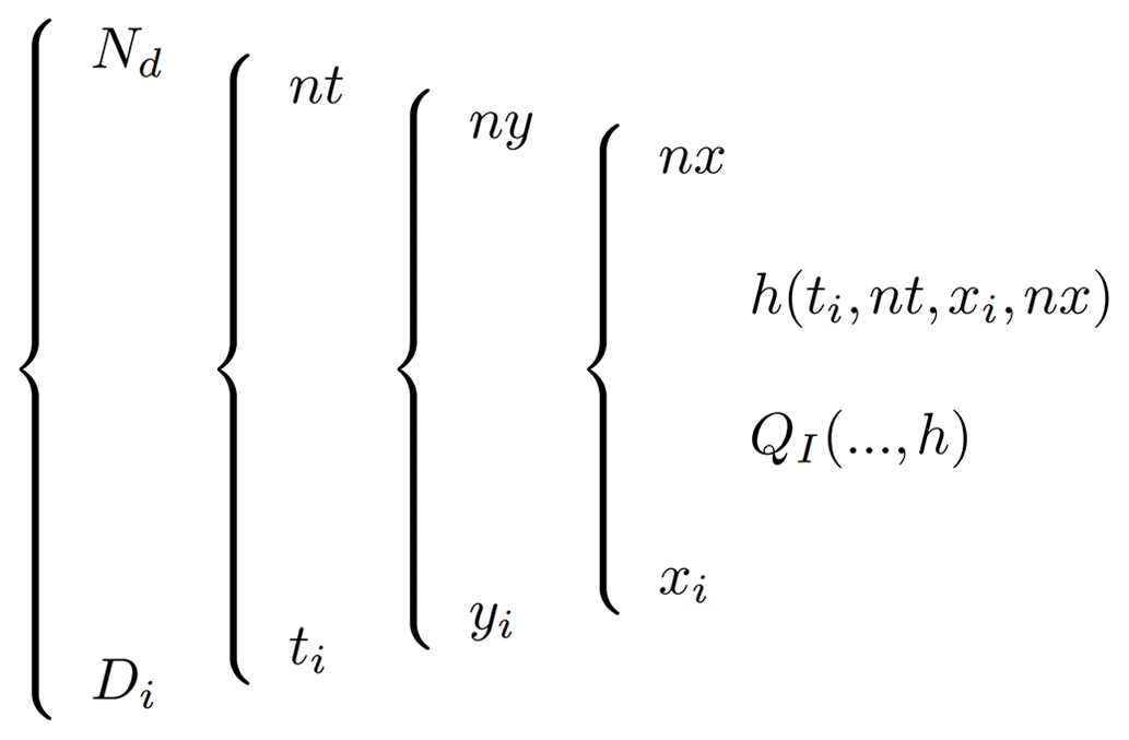
Figure 5An example of the loop employed to run the instantaneous solar radiation subroutine.
In the following, the hour angle, h, is given as a function of the time interval, ti, and longitude, xi:
Therefore, after calculating h, the results must be substituted into Eq. (20), where the other variables may be calculated using the Q0 method, and negative QI values are assumed to be zero. The algorithm for the hour angle is initiated from the west in an eastwards direction following the Earth's rotation about its axis. Thus, considering the first day, D1, and the first hour (00:00 UTC), t1, the hour angle must be calculated globally. This means that an hour angle covering all longitudinal points from the west to the east must be calculated for each latitude. This way, from the first time step, t1, the algorithm starts the second time step, t2, which is the same data calculated previously at t1, after a westward rotation (Fig. 6). Hence, iterations must repeat for 24 h before the start of the second day, D2, where changes in solar declination, δ, and Earth–Sun distance, ρ, must be considered. In summary, this subroutine is responsible for realistically simulating the ISR in the outer atmosphere to ensure that the program is viable for more complex deployments or studies that require accurate simulations of the effect of the day-to-night transition.
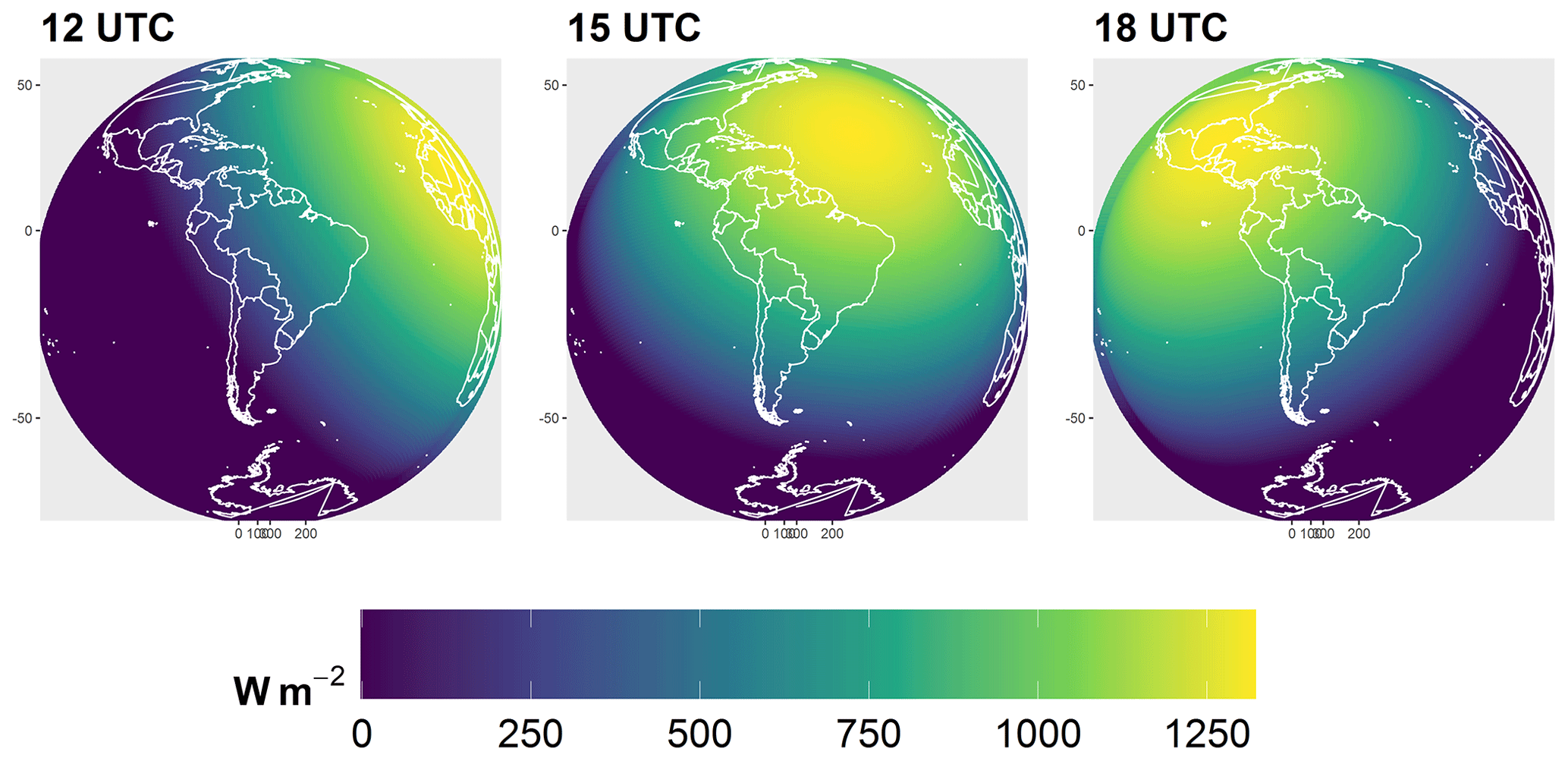
Figure 6The instantaneous solar radiation at the top of the atmosphere from the DINSOL model for the present day on 29 June.
2.4 Orbital motions: parameterizations
The law of universal gravitation computes the mutual attraction force between two bodies, and, according to Yang (2017), their formula is
for the Sun–Earth case. M represents the mass of the Sun, m is the mass of the Earth, G is the universal gravitational constant ( Nm2 kg2), and is a unitary vector. The Earth–Sun distance, a, is given by the average radius of the Earth's orbit.
Although Newton adopted the gravitational law for two celestial bodies with success (e.g. Sun–Earth, Earth–Moon, Sun–Mars), three-body problems proved to be more complex. Precise astronomical predictions require consideration of the gravitational influence of the other celestial bodies (Laskar et al., 2004). Euler and Lagrange found particular solutions for the three-body problem (Musielak and Quarles, 2017). In the late 1880s, Heinrich Bruns and Henri Poincaré showed that a general arrangement of three or more bodies (n-body problem) yielded no analytical solution (Hamilton, 2016).
Though complex astronomical motions cannot admit analytical solutions, a distinguished researcher overcame this obstacle by adopting the spectral decomposition technique. André Berger made it possible for anyone to estimate the Earth's orbital parameters (EOPs) within ±1 Myr of the present (Crucifix et al., 2009). His parameterization was published firstly in Berger (1978b), and after some years, a newer version in Berger and Loutre (1991) expanded the valid time range to ±3 Myr. Now, in this section and the following, Berger (1978b) and Berger and Loutre (1991) are referred to as Be78 and Be90, respectively. Both parameterizations, Be78 and Be90, are described in this section, with a focus on the main formulas and tables presented in this classical paper.
Another remarkable researcher, Jacques Laskar, also simulated new long-term solutions for EOPs. Berger used the Laskar solutions in Be90 (Laskar, 1986, 1988). Furthermore, within the last decades, Laskar published novel solutions focused on expanding the valid time range (e.g. Laskar et al., 1993, 2004, 2011). It is worth mentioning that although current computers can simulate the planetary motions around the Sun for billions of years, the chaotic behaviour of the solution still limits the validation to a few tens of millions of years (Laskar et al., 2011).
Thus, the efforts of André Berger and Jacques Laskar represent an important contribution to paleoclimatology. This way, following the idea of this section, the mathematical description of the Berger parameterizations, ranging from equations to constants, is provided, as well as a Laskar custom parameterization, such as in the DINSOL source code.
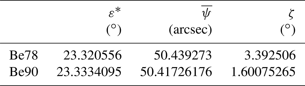
Table 1The constant values are used to solve the Berger parameterizations.
2.4.1 The analytical solution of Be78 and Be90
Both parameterizations, Be78 and Be90, use spectral analysis, which used the same trigonometrical equations. However, the Be78 and Be90 methods require distinctive data sources to work. Thus, DINSOL contains three tables for every Berger parameterization: obliquity, eccentricity, and precession, such as Tables 1, 4, and 5 in Be78, respectively. Furthermore, all these data tables were obtained from an R package named PALINSOL (Crucifix, 2016) and converted to sequential binary files. The data contained the following columns: amplitude, mean rate, phase, and period. The time in years for the Be78 and Be90 parameterizations is represented in the equations by the t variable.
The calculation of the obliquity (ε) is then estimated with the following equation:
where ε* is a constant given in Table 1; N represents the number of terms per column; and Ai, Ri, and Fi are, respectively, the second, third, and fourth columns of the obliquity tables used in Be78 and Be90. Similarly to the obliquity, the eccentricity, e, can be calculated from the following equations:
where Mi, Gi, and Bi are, respectively, the second, third, and fourth columns of the eccentricity tables used in Be78 and Be90, and N is the number of elements per column. To calculate the precession, ϖ, the following these steps must be followed:
where ψ is the general precession, and the constants and ζ are given in Table 1. Pi, Ki, and Di are, respectively, the second, third, and fourth columns of the precession tables used in Be78 and Be90. Moreover, N is the number of table terms. Now, we also need to calculate the arctangent from esin π and ecos π, like Eq. (28).
If arctan π is negative, 180∘ must be added for arctan π or else it must be kept unchanged. The longitude of the perihelion, ϖ, can now be calculated using the following equation:
If ϖ is greater than 360∘, subtraction () must be performed to obtain an angle less than the length of a full revolution. The longitude of perigee, ω, can be calculated as . Additionally, it is crucial use the same units: radians, degrees, and arcseconds. For instance, DINSOL Berger subroutines convert all column data to radians.
2.4.2 The Laskar solutions
The DINSOL model combines two Laskar time series solutions (Laskar et al., 2004, 2011), resulting in a time range from −249 to 21 Myr, referred to as the Lask. It implements the function s(y), where y is a year as a multiple of 1000. However, if y is not a multiple of 1000, s(y) cannot be used directly, and a simple slope–intercept equation must be used where the two nearest points are defined as before (ti) and after (ti+1). For instance, if , then , and . Thus, the effective time, t, used in the slope–intercept equation is , which results in a time of t=400.
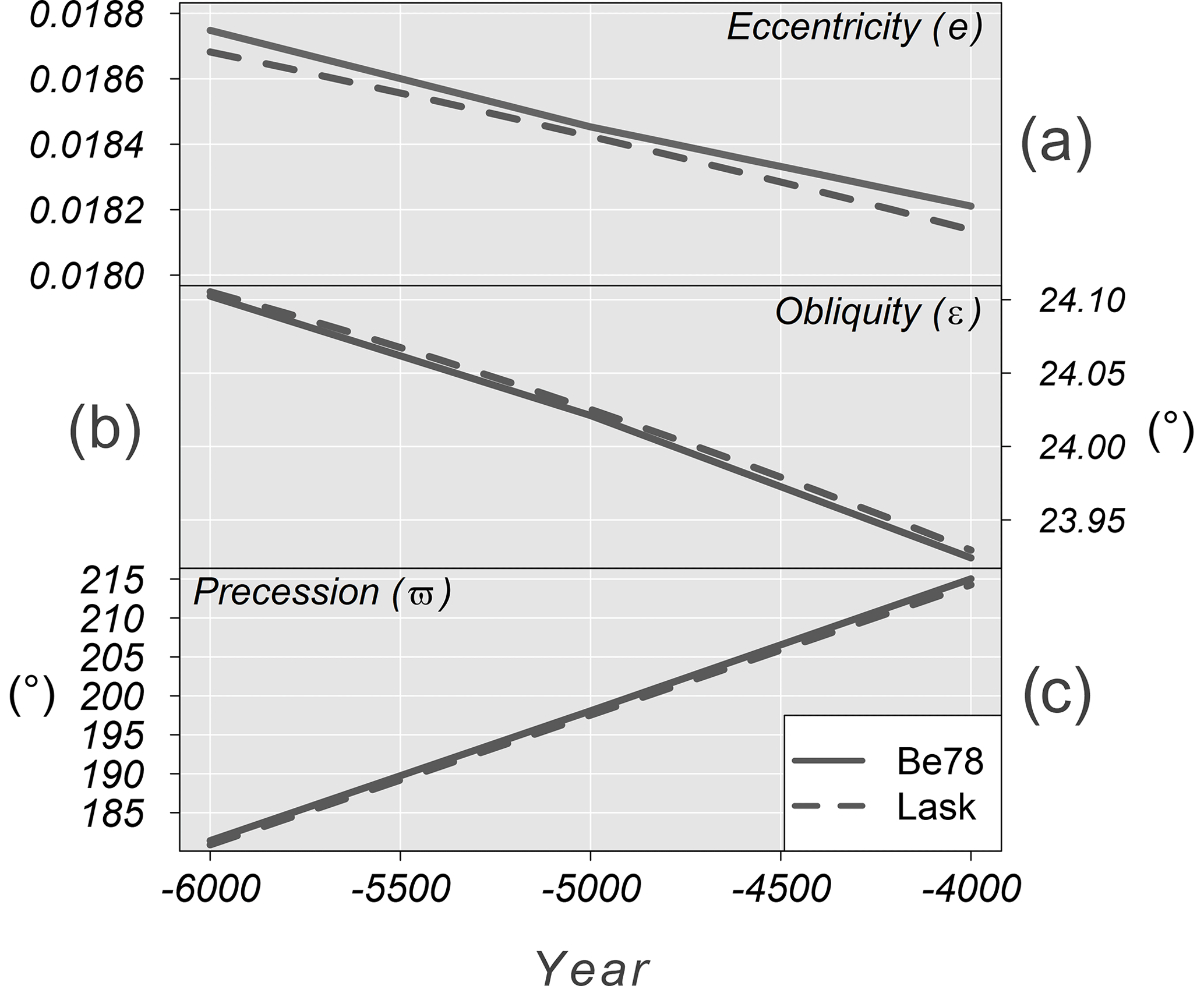
Figure 7Comparison between Be78 and Lask data with time (in years) on the horizontal axis. Additionally, graph (a) is eccentricity, (b) is obliquity (∘), and (c) is precession (∘).
Next, Eq. (30) is shown, where f(y) may assume two forms:
where b=s(ti), and the slope is given by
The annual change for each EOP is small, resulting in a small calculation error from the slope–interception equation. Additionally, comparing the Be78 and Lask data calculated from DINSOL, Fig. 7 shows that the graphs overlap; therefore, the Lask parameterization can accurately estimate the nonexistent original Laskar data. Both Laskar solutions were obtained from the web page http://vo.imcce.fr/insola/earth/online/earth/earth.html (last access: 21 January 2023), which is maintained by the Institut de Mécanique Céleste et de Calcul des Ephémérides (IMCCE).
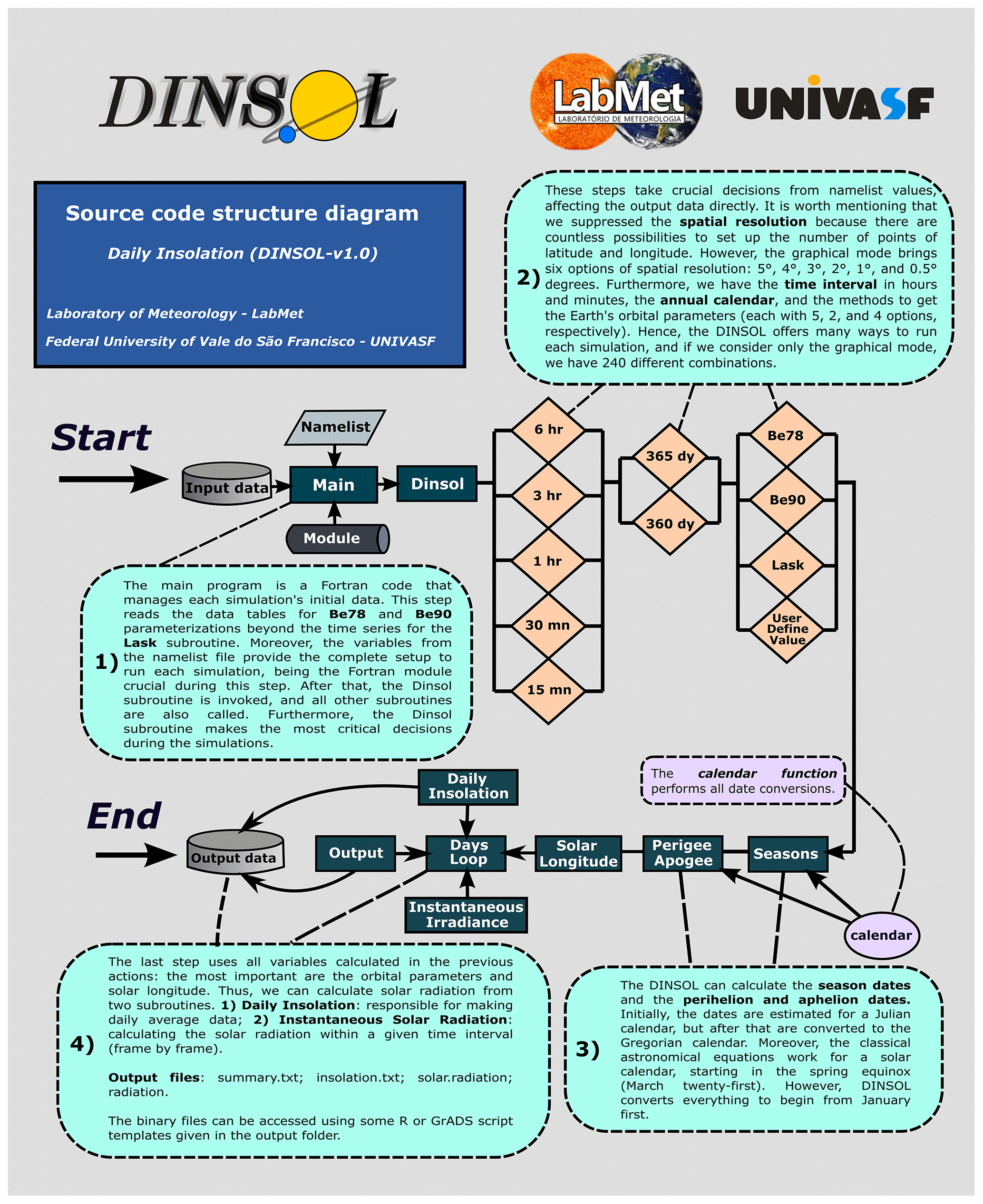
Figure 8Fortran representation of the DINSOL source code, with subroutines, modules, namelist, input and output data, and brief explanations of the simulation steps.
2.5 Model structure, set-up, and execution
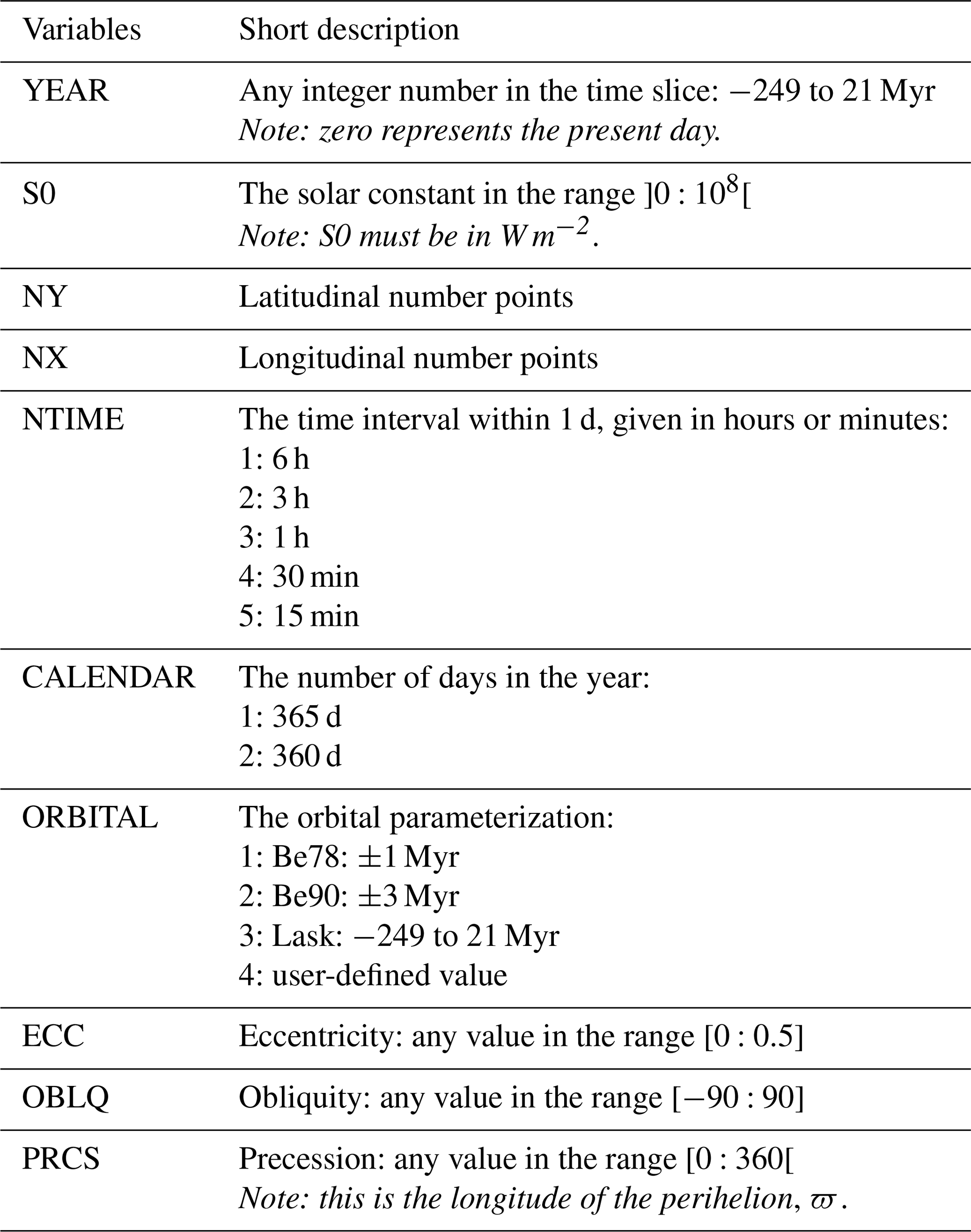
The DINSOL source code has a simple hierarchical structure written in Fortran. A flow diagram representing the DINSOL source code is available in Fig. 8, including input data, the main program, modules, functions, subroutines, and output data. The model is initiated from the main program reading the input data: tables for analytical solutions of Be78 and Be90 and combined time series of Lask. The program also reads data from the namelist file (Table 2) as well as a module containing the declared variables and simulation parameters. In the next step, the program invokes the DINSOL subroutine, which is the main function and calls all other functions for the simulations.
The next steps are a series of commands executed from the namelist set-up function, where the calendar type must be initialized. Variables like spatial resolution, time interval, and calendar variables are then declared. The next step invokes parameterization to obtain the orbital parameters, and then the subroutines (seasons, perigee, and apogee) implement a calendar function to determine the day and month occurrences of summer, autumn, winter, the perihelion, and the aphelion. The solar longitude subroutine is then called and computes the annual true solar longitude for use in the daily insolation and instantaneous irradiance subroutines. Finally, the output subroutine is responsible for storing the data simulated during the DINSOL execution.
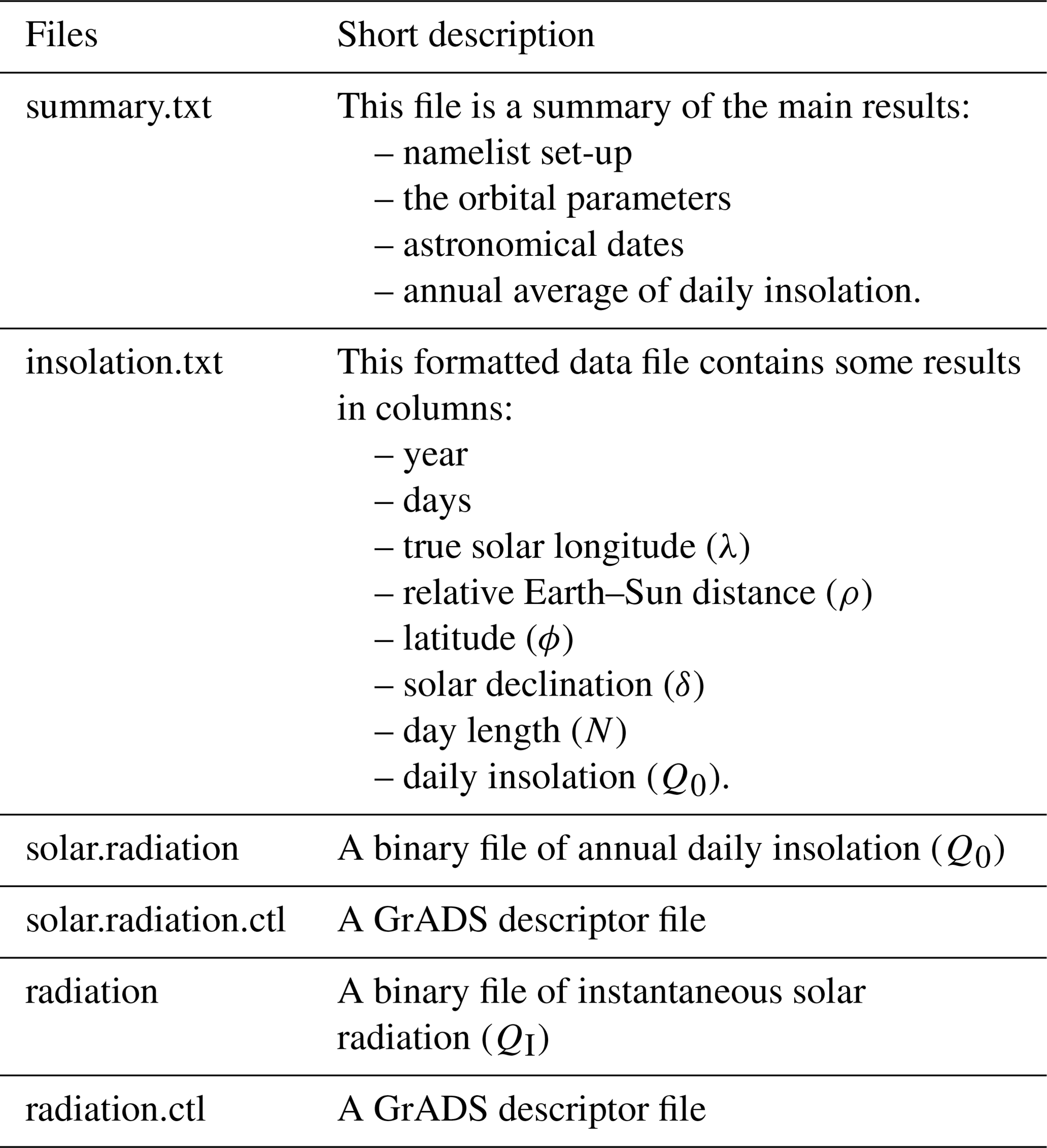
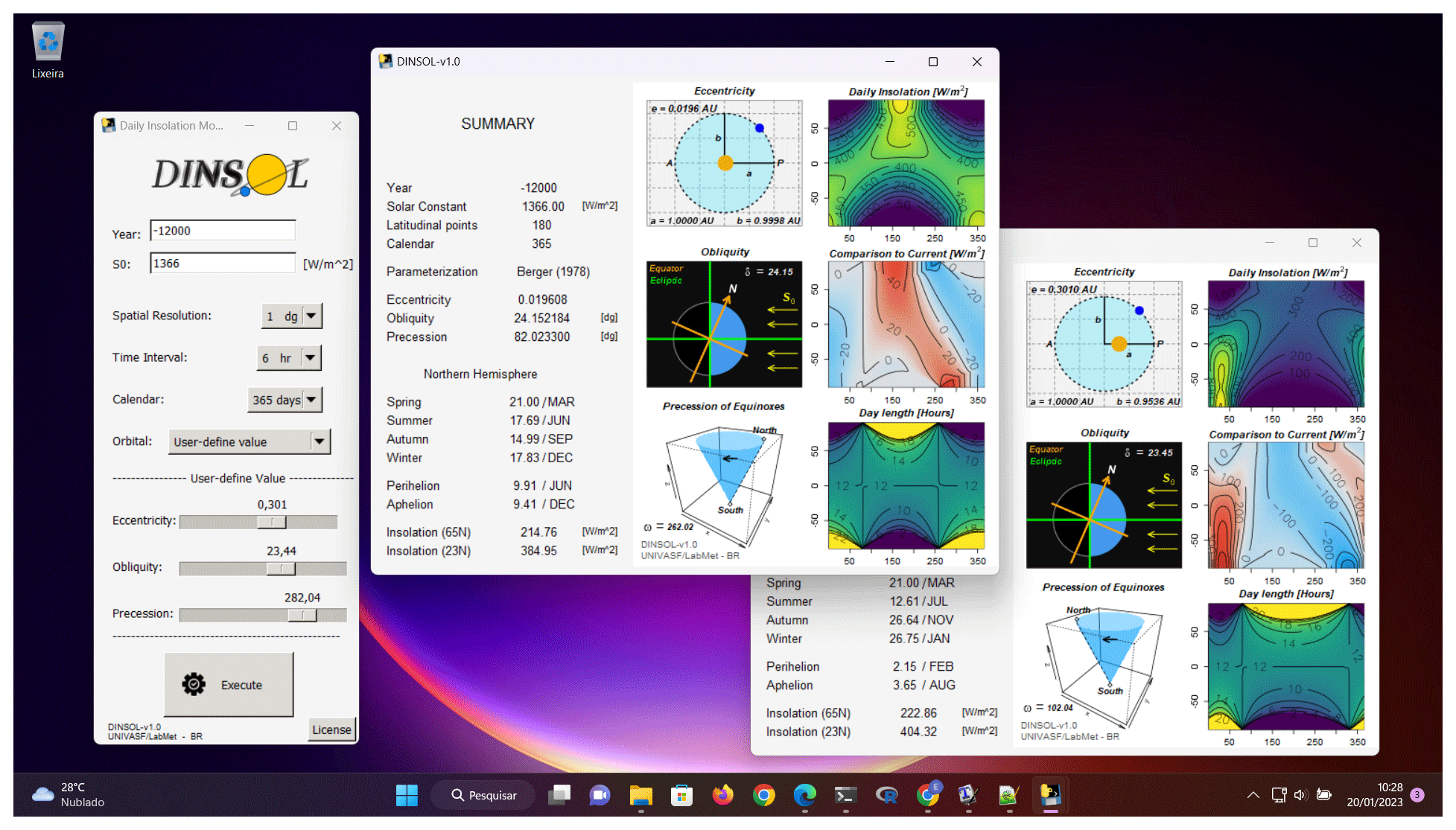
The DINSOL model also works from a GUI, where the namelist options are the same, except for the spatial resolution, where the GUI mode offers only six options: 5, 4, 3, 2, 1, and 0.5∘. All the output files generated (Table 3) are identical regardless of the execution mode, except for the plot file gui-plot.png: a panel used to display results in the GUI mode. This plot contains sketches of the orbital parameters and contour fields for a simulated year: daily insolation, the difference to present day, and the length of a day. A snapshot of the GUI interface and two graphical windows containing the results is displayed in Fig. 9.
Users have the option to customize their simulation set-up, implementing custom scenarios using a user-defined value. The orbital parameters can then be set without compliance to the Berger or Laskar parameterizations, provided that the results will not be invalidated. For instance, if the eccentricity is set to zero, the orbit of Earth would become a perfect circle, meaning the dates of the perihelion and aphelion would no longer exist. If obliquity is set to zero, the seasons would not exist, and if a negative obliquity is assumed, the solstice and equinox dates would occur on inverted dates. Even under hypothetical cases, the program still works correctly.
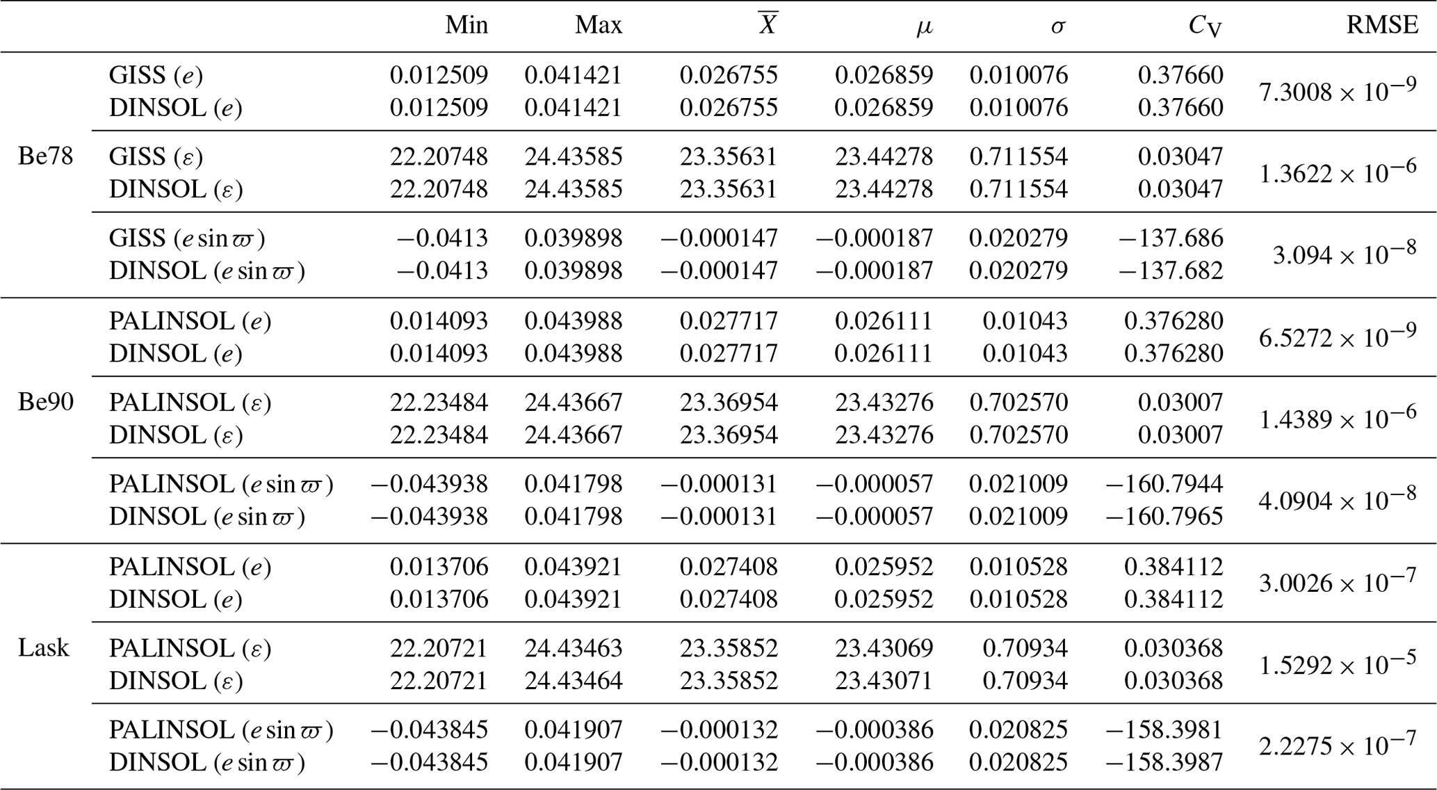
This section evaluates the DINSOL program by comparing its products against data obtained from other similar tools or available in the literature. Still, the first subsection presents the Earth's orbital parameter (EOP) evaluation, where the Be78, Be90, and Lask parameterizations (Sect. 2.4) were evaluated. For that, we compared the Be78 parameterization with the Goddard Institute for Space Studies (GISS) data computed by Bartlein and Shafer (2019a). The authors adapted a set of Fortran programs provided by the GISS that run the EOPs using the Be78 parameterization (Bartlein and Shafer, 2019b). On the other hand, the Be90 and Lask parameterizations were evaluated by adopting the PALINSOL package (Crucifix, 2016). The EOP evaluation assumes a time series' starting from −150 kyr until present day, t=0. Furthermore, we decided to use the climatic precession (esin ϖ) instead of the distance of the perihelion, ϖ.
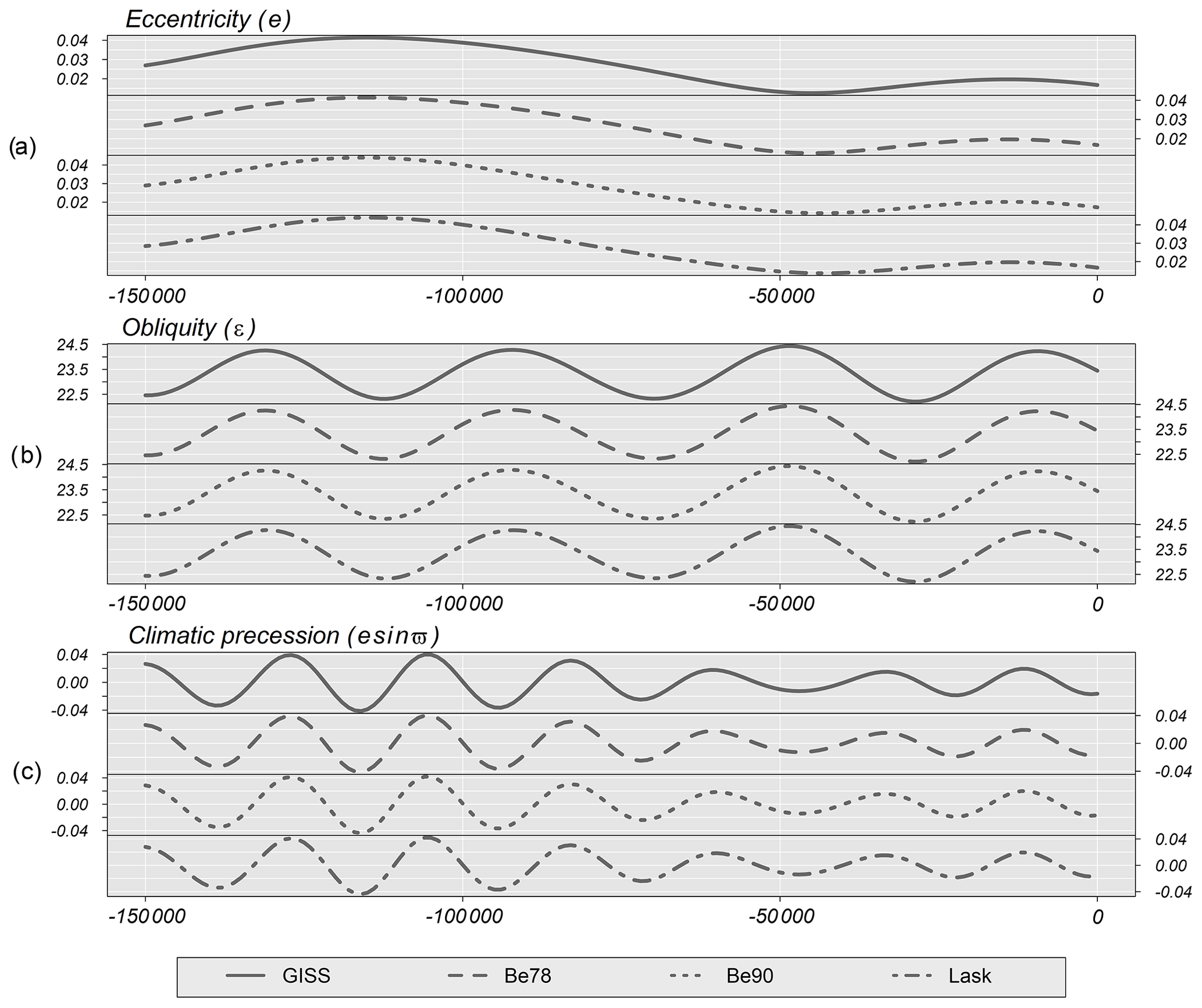
Figure 10Time series of the Earth's orbital parameters (EOPs) for the last 150 kyr. (a) Eccentricity, (b) obliquity, and (c) climatic precession. Each graph shows Goddard Institute for Space Studies (GISS) and DINSOL parameterizations: Be78, Be90, and Lask.
Table 4Evaluation of the DINSOL model adopting a statistical analysis from Earth's orbital parameters (EOPs), where the values are from the minima (Min), maxima (Max), average (), median (μ), standard deviation (σ), coefficient of variation (CV), and the root mean square error (RMSE) of each tool type. All presented data were obtained from DINSOL, GISS, and PALINSOL. The EOPs are the eccentricity (e), obliquity (ε), and climatic precession(esin ϖ).
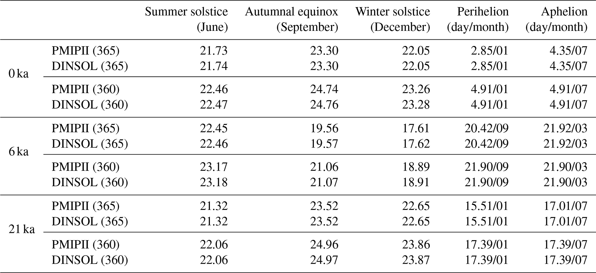
Over the following subsections, we analyse DINSOL compared to PMIPII and PALINSOL. At first, we evaluate the astronomical dates by using the PMIPII dates as a reference. Please note that the classical method of measuring the paleoclimate dates assumes the spring equinox to be a fixed date (21 March) and a constant month length regardless of the year. Still, in the final subsection, the evaluation of the monthly insolation data is conducted, where the assumption is that the solar constant is S0=1365 W m−2, and the year is equal to t=0 for present day (0 ka), during the mid-Holocene (6 ka), and in the Last Glacial Maximum (21 ka) using a 365 and 360 d calendar with the Berger (1978b) parameterizations (EOPs and daily insolation), such as the implemented PMIPII experiments.
The samples were analysed from measures of central tendency using average () and median (μ), as well as measures of dispersion using standard deviation (σ) and coefficient of variation (CV). Additionally, the root mean square error (RMSE) was implemented to evaluate the sample differences, where the RMSE was calculated by performing the sum of the differences between simulation and observational data, given by Eq. (32):
In accordance with Oliveira et al. (2019), N is the number of elements, Si represents the simulation data, and Oi is the observational data. Note that PMIPII, PALINSOL, and GISS are assumed to be observational data, a standard dataset to evaluate DINSOL.
Table 5This table contains the dates of summer, autumn, winter, the perihelion, and the aphelion during present day (0 ka), the mid-Holocene (6 ka), and the Last Glacial Maximum (21 ka) calculated by DINSOL and by PMIPII, both using the method of Be78, for 365 and 360 d calendars.
3.1 Earth's orbital parameters
In Fig. 10, there is a correlation between the GISS and DINSOL curves, indicating that DINSOL EOP subroutines (Be78, Be90, and Lask) function as expected. The error margin estimations were determined using a statistical summary shown in Table 4. Thus, measurements such as mean (), median (μ), standard deviation (σ), and coefficient of variation (CV) indicate a strong correlation between DINSOL and GISS as well as DINSOL and PALINSOL, therefore suggesting an insignificant difference to the EOP DINSOL products. The RMSE values also support the previous statistical inference from the insignificant difference between the samples.
The GISS and Be78 values are nearly identical, which validates the Be78 subroutine. The same occurs with the Be90 and Lask parameterizations, where the test parameters indicate a roundoff error between DINSOL and PALINSOL. In addition, regarding the coefficient of variation, CV, we see that it was the climatic precession (esin ϖ) that showed the more prominent differences. Moreover, we found the largest RMSE value during the Lask evaluation, specifically in the obliquity (ε) parameter. Note that for negative years (reconstructions), DINSOL adopts Laskar et al. (2011) (la10), while PALINSOL adopts Laskar et al. (2004) (la04), which justifies this slight difference.
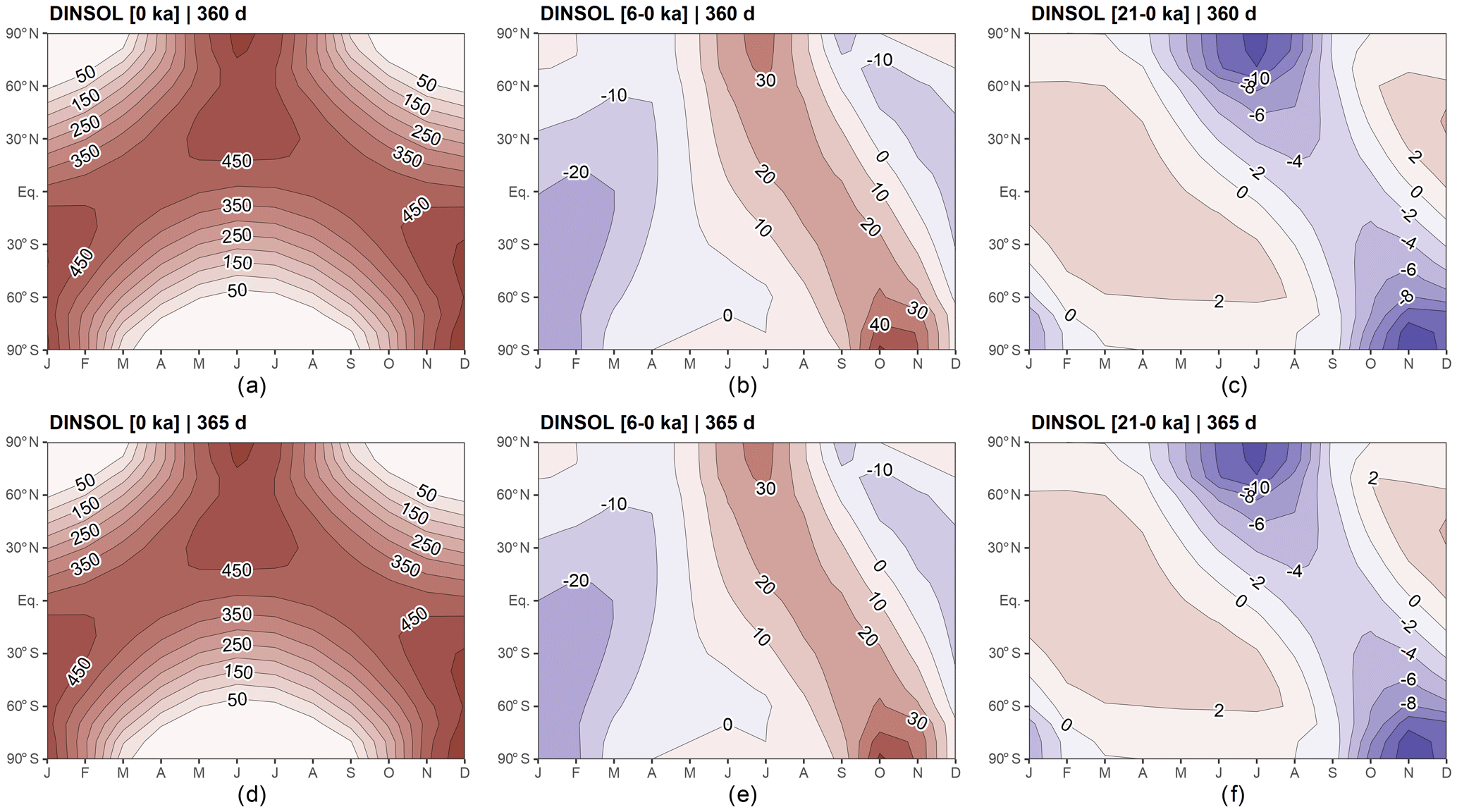
Figure 11DINSOL monthly insolation contour fields obtained from a 360 d calendar – (a) present day, (b) mid-Holocene minus present day, (c) Last Glacial Maximum minus present day – and from a 365 d calendar – (d) present day, (e) mid-Holocene minus present day, (f) Last Glacial Maximum minus present day. The horizontal axis represents the months, while the vertical axis is the latitude.
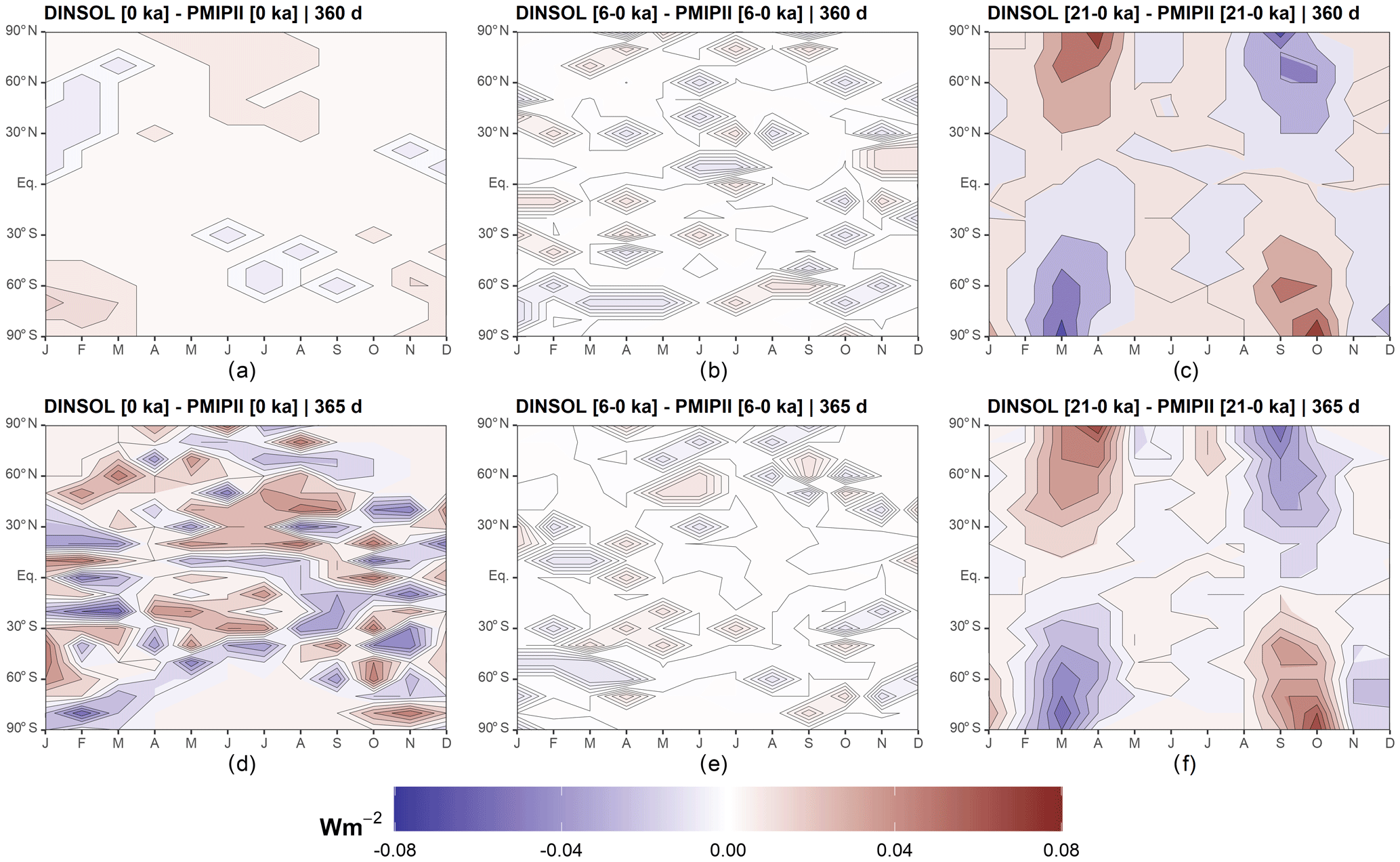
Figure 12Monthly insolation differences between DINSOL and PMIPII from a 360 d calendar – (a) present day, (b) mid-Holocene minus present day, (c) Last Glacial Maximum minus present day – and from a 365 d calendar – (d) present day, (e) mid-Holocene minus present day, (f) Last Glacial Maximum minus present day. The horizontal axis represents the months, while the vertical axis is the latitude.
Although the parameterizations Be78, Be90, and Lask provide almost the same values, the users need to pay attention to the epoch and ecliptic reference used by each parameterization, that is, the time references, which are different from one another. For instance, while Be78 assumed 1950 to be the epoch and 1850 to be its ecliptic reference, the Lask parameterization adopted J2000 as a time reference, conforming to the Julian calendar. Therefore, t=0 represents the year 1950 in Be78 and 2000 in Lask. Thus, to overlap the Be78 and Lask parameterizations, we would need to perform a calibration shift of 50 years one another. For additional information the reader is referred to the Berger and Laskar articles.
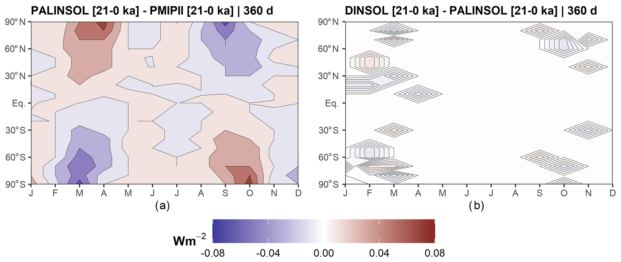
Figure 13Contour fields of monthly insolation from Last Glacial Maximum minus present day: (a) PALINSOL minus PMIPII and (b) DINSOL minus PALINSOL. Each one is for a 360 d calendar. The horizontal axis represents the months, while the vertical axis is the latitude.
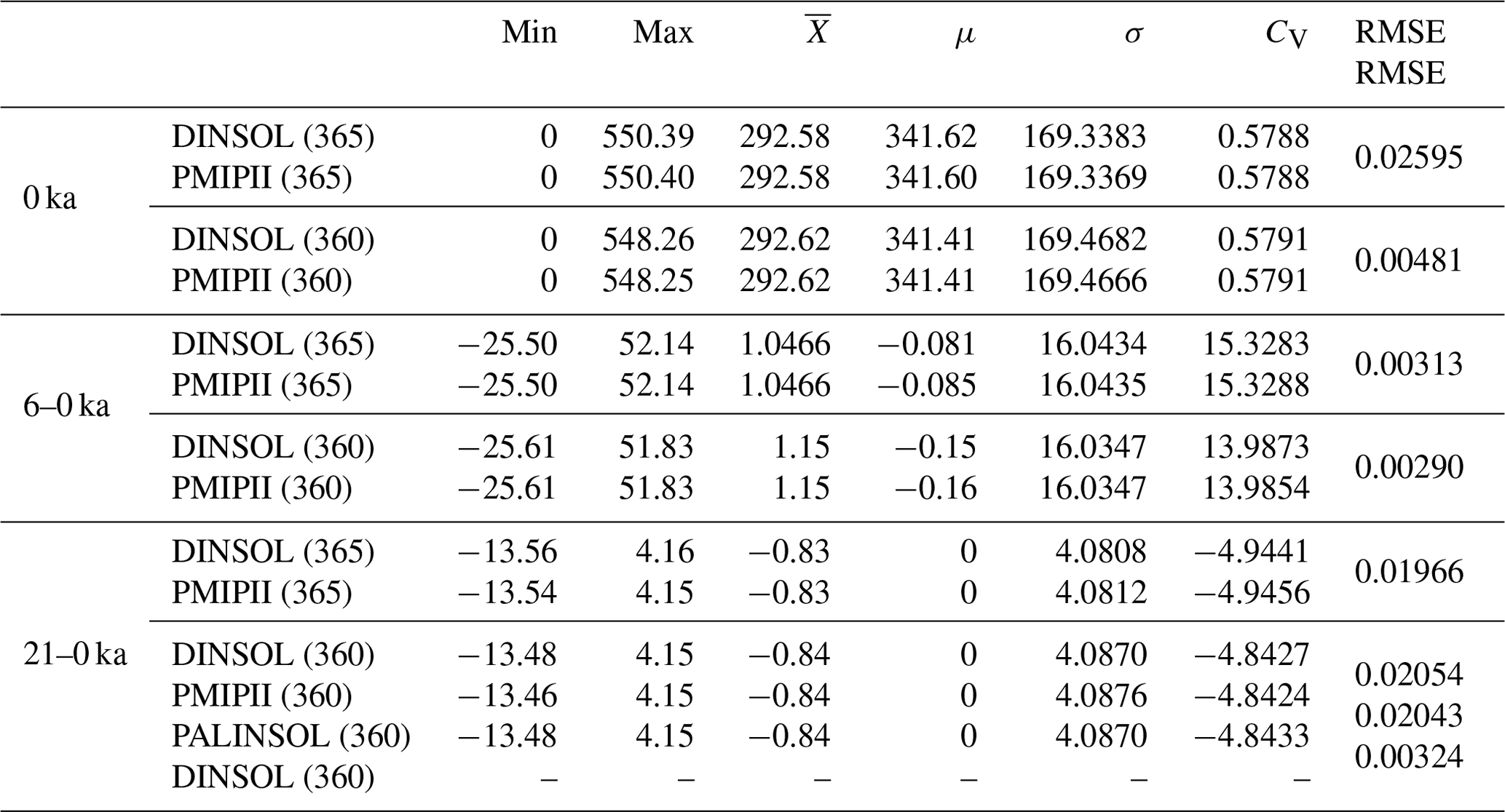
Table 6Evaluation of the DINSOL model adopting a statistical analysis from monthly insolation data samples, where the data displayed represent the minimum values (Min), maximum values (Max), average (), median (μ), standard deviation (σ), coefficient of variation (CV), and the root mean square error (RMSE). All presented data were obtained from DINSOL, PMIPII, and PALINSOL. They have two calendar options (365 and 360 d) and three different periods: present day (0 ka), the mid-Holocene (6–0 ka), and the Last Glacial Maximum (21–0 ka).
3.2 Astronomical dates
Table 5 contains the dates of summer, autumn, winter, the perihelion, and the aphelion calculated by DINSOL and PMIPII, where both use the method of Be78. These dates represent present day (0 ka), the mid-Holocene (6 ka), and the Last Glacial Maximum (21 ka). Thus, perihelion and aphelion dates calculated by DINSOL are identical to those calculated by PMIPII. These dates correlate with the expected dates because they were determined using Eqs. (4), (5), and (6). Nevertheless, the summer, autumn, and winter dates have a small error compared to those determined by PMIPII. In DINSOL, these dates were estimated from a large number of values within the annual true solar longitude vector. In Table 5, an accumulative error is observed, where the season date error increases as a function of the distance to the spring equinox. The RMSE provides values around 12, 16, and 19 min for summer, autumn, and winter, respectively. Thus, for less than 20 min, the error remains small, meaning that DINSOL provides accurate date estimates. The compliance of DINSOL and PMIPII to the classical method of measuring astronomical events must always be considered. However, for a more realistic approach to paleoclimate calendars, it is recommended to follow the methodology of Joussaume and Braconnot (1997) or Bartlein and Shafer (2019a), although many authors prefer the classical method because it is easier to compare with our current Gregorian calendar.
3.3 Monthly insolation
The DINSOL monthly insolation was analysed from a visual evaluation of the contour fields (Figs. 11, 12, 13) and some statistical parameters (Table 6). This evaluation used PMIPII insolation samples prepared from 365 and 360 d calendars for three different periods: present day (0 ka), the mid-Holocene (6–0 ka), and the Last Glacial Maximum (21–0 ka). Simulations were thus performed with DINSOL using the same PMIPII set-up. Additionally, DINSOL was compared to the monthly insolation obtained from the PALINSOL package, but, in this case, we considered only the Last Glacial Maximum (21–0 ka) period. Incidentally, the contour fields present in Fig. 11a–c were generated using a 360 d calendar, with d–f employing a 365 d calendar set-up. From Fig. 11, compared to present day, the biggest insolation differences were found during the mid-Holocene, primarily due to the perihelion date changes, around 3 January for present day and 20 September during the mid-Holocene. This analysis of the mid-Holocene agrees with the presented discussion in Brierley et al. (2020).
In order to perform the visual evaluation, we plotted the contour fields of DINSOL minus PMIPII (Fig. 12). Thus, in Fig. 12a–c, we have contour fields made from a 360 d calendar, whereas Fig. 12d–f is based on a 365 d calendar. Still, it is clear that for present day (0 ka), the mid-Holocene (6 ka), and the Last Glacial Maximum (21 ka), the differences are within the roundoff error, about ±0.08 W m−2. Figure 12a, b, and e contain plots almost uniform with values nearest to zero than the other panels. For example, Fig. 12d presents a more remarkable bias. However, it is worth noting that the values are randomly distributed in the image, which is considered normal and allows us to infer that DINSOL is working according to the expectations of present day (0 ka) and the mid-Holocene (6 ka), including both calendar options: 360 and 365 d.
On the other hand, Fig. 12c and f show a systematic bias for high latitudes, where we can observe an almost harmonic behaviour between the Northern Hemisphere and Southern Hemisphere, which happens near the equinox dates. Despite that, the differences remain small, and as a confirmation test, we additionally decided to compare PMIPII (21–0 ka) to PALINSOL. Moreover, we also performed a DINSOL and PALINSOL comparison to the Last Glacial Maximum. Thus, Fig. 13a shows the same pattern at high latitudes, whereas Fig. 13b plots an almost uniform field. Therefore, DINSOL minus PALINSOL works as expected, suggesting that PMIPII (21–0 ka) contains some systematic roundoff error in the monthly insolation files, which should be reported to the PMIP team in order to investigate it.
With regard to the statistical analyses, the parameters available in Table 6 are dependable enough to confirm or reject our previous visual analyses from Figs. 11, 12, and 13. At first, we can see that the minima and maxima are nearly identical and converge towards the same value in the mid-Holocene. Furthermore, the central tendency indicates that all samples' average values are equal, while most median values are almost identical. The dispersion values also corroborate the previous conclusions, where the standard deviation and coefficient of variation suggest no significant differences. Still, in order to estimate the error between DINSOL and PMIPII samples, we also compute the RMSE. Table 6 shows that the highest value occurred from a calendar of 365 d when assaying present day, 0.02595 W m−2. On the other hand, a lower RMSE value was found for a calendar of 360 d by considering the mid-Holocene sample.
As a final analysis, we focus on the Last Glacial Maximum, including the PALINSOL package as an alternative to the PMIPII samples. Thus, comparing PALINSOL and PMIPII, we realized that the RMSE was almost identical to the DINSOL and PMIPII values. However, evaluating DINSOL from PALINSOL, we got an RMSE of 0.00324 W m−2, which is around 84 % less than the value obtained from DINSOL and PMIPII analyses. Therefore, it is reasonable to claim that the DINSOL program can compute the daily insolation accurately compared to the literature because the field differences show us almost homogenous contour data with values near zero. Indeed, according to Table 6, all samples must be considered numerically the same because we did not find significant differences in our statistical analyses.
The Daily INSOLation (DINSOL-v1.0) program is a robust and versatile tool offering various simulation options and usability. It is ideal to compute solar radiation data for climate models, which aids in simplified climate approaches or more complex studies. Furthermore, the DINSOL model may be employed as an educational tool by adopting its user-friendly GUI. The program was developed as a novel educational tool for use in geoscience colleges worldwide, providing a quick view of daily insolation by considering the Milankovitch cycles (ideal for paleoclimatology) or adopting hypothetical orbital parameters (ideal for exoplanets). Therefore, the program can aid students, teachers, and researchers in conducting their respective studies. Still, despite the program evaluation having presented insignificant differences compared to the literature, the users are incentivized to report any issues found during the program execution. Moreover, DINSOL is an open-source program whose author encourages users to develop the source code continuously. Ultimately, DINSOL may be considered a viable tool that accurately provides various types of output data, such as the Earth's orbital parameters; astronomical dates; daily insolation; and instantaneous solar radiation, simulating the passage of day to night realistically.
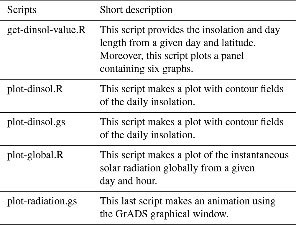
The output folder contains five scripts to aid users in analysing the simulation data. The files are listed with a brief description in Table A1.
Table A1Brief description of all scripts located in the DINSOL output folder.
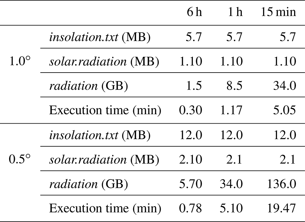
DINSOL does not adopt restrictions for latitudinal and longitudinal number points during execution by command lines, which means that the high-resolution set-ups demand users' attention. This appendix brings a table containing the output file sizes for different simulation set-ups, where the instantaneous solar radiation file (radiation) grows significantly as a function of the time interval (hours or minutes) and spatial resolution. Thus, it is necessary to ensure that the computer has sufficient storage capacity in its hard disk prior to conducting a high-resolution simulation; otherwise, the system could crash, interrupting the simulation. It is worth mentioning that most data visualization tools cannot allocate enormous files. Thus, to get around this, the user should use some tool like the Climate Data Operator (CDO) to extract a specific hour of the day and perform some plot analysis posteriorly. Another question is the execution time, which is increasing substantially and is a function of the computational power, compiler, program set-up, etc. In addition, even though the standard source code works only in serial execution, the author already adapted and tested the code to work in parallel using the OpenMP API, which improved the program performance significantly. Please note that when the radiation file is not required, the simulation parameters can be set to NX = 1 and NTIME = 1, allowing users to change the values of NY while keeping simulation times minimal. In any case, the most efficient option would be to modify the source code, deactivating the instantaneous solar radiation subroutine and not storing the radiation data.
Table B1DINSOL short performance summary by considering the spatial resolution and time interval changes, where the computation was performed in the Ubuntu operating system using the IFORT 13 compiler. Thus, we have the required machine storage for each output file as well as the execution time.
The DINSOL program is available for download in different repositories: Zenodo, GitHub, and LabMet/UNIVASF. Further, even though the program is Linux/Unix software, a custom Windows OS version is available too. Both versions (Windows and Linux) contain manuals and README files to aid users in installing the dependencies and compiling the source code. On Zenodo, the Windows version is available at https://doi.org/10.5281/zenodo.7554620 (Oliveira, 2022c), while the Linux version is available at https://doi.org/10.5281/zenodo.7551458 (Oliveira, 2022b). GitHub provides only the Linux version: https://github.com/Emerson-D-Oliveira/dinsol-v1.0-linux (last access: 20 January 2023; DOI: https://doi.org/10.5281/zenodo.7843723, Oliveira, 2023). It is important to mention that the Windows version does not require any prior programming experience from the user to install and execute DINSOL from the GUI mode. Moreover, although the program has not been tested on macOS, the Linux version should work since some adjustments have been made. Ultimately, users are encouraged to adapt and share the modified source code with the community. A supplementary file containing all datasets used to prepare this paper is available in the Zenodo repository (https://doi.org/10.5281/zenodo.7557354; Oliveira, 2022a).
The supplement related to this article is available online at: https://doi.org/10.5194/gmd-16-2371-2023-supplement.
EDO independently wrote all DINSOL source code, scripts, and manuals as well as this paper.
The author has declared that there are no competing interests.
Publisher’s note: Copernicus Publications remains neutral with regard to jurisdictional claims in published maps and institutional affiliations.
The author thanks Michel Crucifix, André Berger, and Jacques Laskar for providing the input data used in the DINSOL parameterizations. In addition, the author also thanks Patrick Bartlein for providing the time series of the Earth's orbital parameters; the Paleoclimate Modelling Intercomparison Project (PMIP) team for providing the monthly insolation data; and the PALINSOL author, whose package was crucial to perform a confirmation test. The author also thanks Kevin Schwarzwald and the referees for the valuable comments regarding the software and the article during the public discussion stage. Their suggestions and observations were fundamental to improving the article's quality. Moreover, the author is grateful to the topical editor Travis O'Brien and the whole journal editorial team. Finally, the author thanks the Federal University of Vale do São Francisco (UNIVASF) and the Laboratory of Meteorology (LabMet) for incentivizing the development of DINSOL-v1.0.
This paper was edited by Travis O'Brien and reviewed by two anonymous referees.
Bartlein, P. J. and Shafer, S. L.: Paleo calendar-effect adjustments in time-slice and transient climate-model simulations (PaleoCalAdjust v1.0): impact and strategies for data analysis, Geosci. Model Dev., 12, 3889–3913, https://doi.org/10.5194/gmd-12-3889-2019, 2019a. a, b, c
Bartlein, P. and Shafer, S.: pjbartlein/PaleoCalAdjust: PaleoCalAdjust v1.0d (v1.0d), Zenodo [data set], https://doi.org/10.5281/zenodo.3386427, 2019b. a
Berger, A.: Obliquity and general precession for the last 5 000 000 years, Astron. Astrophys., 51, 127–135, 1976. a
Berger, A.: Long-term variations of the Earth’s orbital elements, Celestial Mech., 15, 53–74, 1977. a
Berger, A.: Long-term variations of daily insolation and Quaternary, J. Atmos. Sci., 35, 2362–2367, 1978a. a
Berger, A.: Long-term variations of caloric insolation resulting from the Earth’s orbital elements, Quaternary Res., 9, 139–167, 1978b. a, b, c, d, e, f, g, h, i, j, k, l
Berger, A.: Milankovitch, the father of paleoclimate modeling, Clim. Past, 17, 1727–1733, https://doi.org/10.5194/cp-17-1727-2021, 2021. a, b
Berger, A. and Loutre, M.: Insolation values for the climate of the last 10 million years, Quaternary Sci. Rev., 10, 297–317, https://doi.org/10.1016/0277-3791(91)90033-Q, 1991. a, b, c, d
Berger, A., Loutre, M.-F., and Yin, Q.: Total irradiation during any time interval of the year using elliptic integrals, Quaternary Sci. Rev., 29, 1968–1982, https://doi.org/10.1016/j.quascirev.2010.05.007, 2010. a, b
Beutler, G.: Methods of Celestial Mechanics, 1st edn., Springer Berlin, Heidelberg, ISBN: 978-3-540-26870-3, https://doi.org/10.1007/b138225, 2005. a
Borkowski, K. M.: The Persian Calendar for 3000 Years, Earth Moon Planets, 74, 223–230, https://doi.org/10.1007/BF00055188, 1996. a
Brierley, C. M., Zhao, A., Harrison, S. P., Braconnot, P., Williams, C. J. R., Thornalley, D. J. R., Shi, X., Peterschmitt, J.-Y., Ohgaito, R., Kaufman, D. S., Kageyama, M., Hargreaves, J. C., Erb, M. P., Emile-Geay, J., D'Agostino, R., Chandan, D., Carré, M., Bartlein, P. J., Zheng, W., Zhang, Z., Zhang, Q., Yang, H., Volodin, E. M., Tomas, R. A., Routson, C., Peltier, W. R., Otto-Bliesner, B., Morozova, P. A., McKay, N. P., Lohmann, G., Legrande, A. N., Guo, C., Cao, J., Brady, E., Annan, J. D., and Abe-Ouchi, A.: Large-scale features and evaluation of the PMIP4-CMIP6 midHolocene simulations, Clim. Past, 16, 1847–1872, https://doi.org/10.5194/cp-16-1847-2020, 2020. a, b
Crucifix, M.: palinsol : a R package to compute Incoming Solar Radiation (insolation) for palaeoclimate studies, Zenodo [code], https://doi.org/10.5281/zenodo.7198545, 2016. a, b
Crucifix, M., Claussen, M., Ganssen, G., Guiot, J., Guo, Z., Kiefer, T., Loutre, M.-F., Rousseau, D.-D., and Wolff, E.: Preface “Climate change: from the geological past to the uncertain future – a symposium honouring André Berger”, Clim. Past, 5, 707–711, https://doi.org/10.5194/cp-5-707-2009, 2009. a, b
Eyring, V., Bony, S., Meehl, G. A., Senior, C. A., Stevens, B., Stouffer, R. J., and Taylor, K. E.: Overview of the Coupled Model Intercomparison Project Phase 6 (CMIP6) experimental design and organization, Geosci. Model Dev., 9, 1937–1958, https://doi.org/10.5194/gmd-9-1937-2016, 2016. a
Fischer, H., van den Broek, K. L., Ramisch, K., and Okan, Y.: When IPCC graphs can foster or bias understanding: evidence among decision-makers from governmental and non-governmental institutions, Environ. Res. Lett., 15, 114041, https://doi.org/10.1088/1748-9326/abbc3c, 2020. a
Fu, W. Q.: 4 – Radiative Transfer, in: Atmospheric Science, second edn., edited by: Wallace, J. M. and Hobbs, P. V., Academic Press, San Diego, 113–152, https://doi.org/10.1016/B978-0-12-732951-2.50009-0, 2006. a
Hamilton, D. P.: Fresh solutions to the four-body problem, Nature, 533, 187–188, https://doi.org/10.1038/nature17896, 2016. a
Hartmann, D. L.: Global Physical Climatology, second edn., Elsevier Science, ISBN 978-0-12-328531-7, https://doi.org/10.1016/C2009-0-00030-0, 2016. a, b
Joussaume, S. and Braconnot, P.: The Persian Calendar for 3000 Years, J. Geophys. Res., 102, 1943–1956, https://doi.org/10.1029/96JD01989, 1997. a, b, c
Jungclaus, J. H., Bard, E., Baroni, M., Braconnot, P., Cao, J., Chini, L. P., Egorova, T., Evans, M., González-Rouco, J. F., Goosse, H., Hurtt, G. C., Joos, F., Kaplan, J. O., Khodri, M., Klein Goldewijk, K., Krivova, N., LeGrande, A. N., Lorenz, S. J., Luterbacher, J., Man, W., Maycock, A. C., Meinshausen, M., Moberg, A., Muscheler, R., Nehrbass-Ahles, C., Otto-Bliesner, B. I., Phipps, S. J., Pongratz, J., Rozanov, E., Schmidt, G. A., Schmidt, H., Schmutz, W., Schurer, A., Shapiro, A. I., Sigl, M., Smerdon, J. E., Solanki, S. K., Timmreck, C., Toohey, M., Usoskin, I. G., Wagner, S., Wu, C.-J., Yeo, K. L., Zanchettin, D., Zhang, Q., and Zorita, E.: The PMIP4 contribution to CMIP6 – Part 3: The last millennium, scientific objective, and experimental design for the PMIP4 past1000 simulations, Geosci. Model Dev., 10, 4005–4033, https://doi.org/10.5194/gmd-10-4005-2017, 2017. a
Kageyama, M., Braconnot, P., Harrison, S. P., Haywood, A. M., Jungclaus, J. H., Otto-Bliesner, B. L., Peterschmitt, J.-Y., Abe-Ouchi, A., Albani, S., Bartlein, P. J., Brierley, C., Crucifix, M., Dolan, A., Fernandez-Donado, L., Fischer, H., Hopcroft, P. O., Ivanovic, R. F., Lambert, F., Lunt, D. J., Mahowald, N. M., Peltier, W. R., Phipps, S. J., Roche, D. M., Schmidt, G. A., Tarasov, L., Valdes, P. J., Zhang, Q., and Zhou, T.: The PMIP4 contribution to CMIP6 – Part 1: Overview and over-arching analysis plan, Geosci. Model Dev., 11, 1033–1057, https://doi.org/10.5194/gmd-11-1033-2018, 2018. a
Klippel, L., St. George, S., Büntgen, U., Krusic, P. J., and Esper, J.: Differing pre-industrial cooling trends between tree rings and lower-resolution temperature proxies, Clim. Past, 16, 729–742, https://doi.org/10.5194/cp-16-729-2020, 2020. a
Kostadinov, T. S. and Gilb, R.: Earth Orbit v2.1: a 3-D visualization and analysis model of Earth's orbit, Milankovitch cycles and insolation, Geosci. Model Dev., 7, 1051–1068, https://doi.org/10.5194/gmd-7-1051-2014, 2014. a
Laskar, J.: Secular terms of classical planetary therories using the results of general theory, Astron. Astrophys., 157, 59–70, 1986. a
Laskar, J.: Secular evolution of the solar system over 10 million years, Astron. Astrophys., 198, 341–362, 1988. a, b
Laskar, J., Joutel, F., and Boudin, F.: Orbital, precessional, and insolation quantities for the earth from −20 Myr to +10 Myr, Astron. Astrophys., 270, 522–533, 1993. a, b
Laskar, J., Robutel, P., Joutel, F., Gastineau, M., Correia, A. C. M., and Levrard, B.: A long-term numerical solution for the insolation quantities of the Earth, Astron. Astrophys., 428, 261–285, https://doi.org/10.1051/0004-6361:20041335, 2004. a, b, c, d, e, f, g
Laskar, J., Fienga, A., Gastineau, M., and Manche, H.: La2010: a new orbital solution for the long-term motion of the Earth, Astron. Astrophys., 532, A89, https://doi.org/10.1051/0004-6361/201116836, 2011. a, b, c, d, e
Lhardy, F., Bouttes, N., Roche, D. M., Abe-Ouchi, A., Chase, Z., Crichton, K. A., Ilyina, T., Ivanovic, R., Jochum, M., Kageyama, M., Kobayashi, H., Liu, B., Menviel, L., Muglia, J., Nuterman, R., Oka, A., Vettoretti, G., and Yamamoto, A.: A First Intercomparison of the Simulated LGM Carbon Results Within PMIP-Carbon: Role of the Ocean Boundary Conditions, Paleoceanography and Paleoclimatology, 36, e2021PA004302, https://doi.org/10.1029/2021PA004302, 2021. a
Liou, K. N.: An Introduction to Atmospheric Radiation, 2nd edn., International Geophysics, Volume 84, Academic Press, https://www.sciencedirect.com/bookseries/international-geophysics/vol/84/suppl/C (last access: 18 April 2023), 2002. a
Menviel, L., Capron, E., Govin, A., Dutton, A., Tarasov, L., Abe-Ouchi, A., Drysdale, R. N., Gibbard, P. L., Gregoire, L., He, F., Ivanovic, R. F., Kageyama, M., Kawamura, K., Landais, A., Otto-Bliesner, B. L., Oyabu, I., Tzedakis, P. C., Wolff, E., and Zhang, X.: The penultimate deglaciation: protocol for Paleoclimate Modelling Intercomparison Project (PMIP) phase 4 transient numerical simulations between 140 and 127 ka, version 1.0, Geosci. Model Dev., 12, 3649–3685, https://doi.org/10.5194/gmd-12-3649-2019, 2019. a, b
Musielak, Z. and Quarles, B.: Three Body Dynamics and Its Applications to Exoplanets, 1st edn., Springer Cham, ISBN 978-3-319-58226-9, https://doi.org/10.1007/978-3-319-58226-9, 2017. a
Oliveira, E. D. and Fernandez, J. H.: Global resolved energy balance with galactic cosmic rays (greb-gcr) theory: a new simplified climate model, Revista Brasileira de Geografia Física, 13, 842–854, https://doi.org/10.26848/rbgf.v13.2.p842-854, 2020. a
Oliveira, E. D., Fernandez, J. H., Mendes, D., Constantino, M. H., and Gonçalves, W. A.: Validation of a simplified climate model adapted to simulate the effects of increased CO2 concentration associated with the galactic cosmic rays theory, Revista Brasileira de Geografia Física, 12, 768–778, https://doi.org/10.26848/rbgf.v12.3.p768-778, 2019. a
Oliveira, E. D.: Supplementary files/DINSOL-v1.0 (1.1), Zenodo [data set], https://doi.org/10.5281/zenodo.7557354, 2022a. a
Oliveira, E. D.: Daily INSOLation (DINSOL-v1.0) program – Linux version (1.0), Zenodo [code], https://doi.org/10.5281/zenodo.7551458, 2022b. a
Oliveira, E. D.: Daily INSOLation (DINSOL-v1.0) program – Windows version (1.0), Zenodo [code], https://doi.org/10.5281/zenodo.7554620, 2022c. a
Oliveira, E. D.: Emerson-D-Oliveira/dinsol-v1.0-linux: dinsol-v1.0-linux (dinsol-v1.0), Zenodo [data set], https://doi.org/10.5281/zenodo.7843723, 2023. a
Otto-Bliesner, B. L., Braconnot, P., Harrison, S. P., Lunt, D. J., Abe-Ouchi, A., Albani, S., Bartlein, P. J., Capron, E., Carlson, A. E., Dutton, A., Fischer, H., Goelzer, H., Govin, A., Haywood, A., Joos, F., LeGrande, A. N., Lipscomb, W. H., Lohmann, G., Mahowald, N., Nehrbass-Ahles, C., Pausata, F. S. R., Peterschmitt, J.-Y., Phipps, S. J., Renssen, H., and Zhang, Q.: The PMIP4 contribution to CMIP6 – Part 2: Two interglacials, scientific objective and experimental design for Holocene and Last Interglacial simulations, Geosci. Model Dev., 10, 3979–4003, https://doi.org/10.5194/gmd-10-3979-2017, 2017. a
Puetz, S. J., Prokoph, A., and Borchardt, G.: Evaluating alternatives to the Milankovitch theory, J. Stat. Plan. Infer., 170, 158–165, https://doi.org/10.1016/j.jspi.2015.10.006, 2016. a
Yang, X.-S.: Chapter 28 – Mathematical Modeling, in: Engineering Mathematics with Examples and Applications, edited by: Yang, X.-S., Academic Press, 325–340, https://doi.org/10.1016/B978-0-12-809730-4.00037-9, 2017. a
- Abstract
- Introduction
- Astronomical aspects and model description
- Model evaluation: a short statistical analysis
- Conclusions
- Appendix A: Data manipulation
- Appendix B: Computing power
- Code and data availability
- Author contributions
- Competing interests
- Disclaimer
- Acknowledgements
- Review statement
- References
- Supplement