the Creative Commons Attribution 4.0 License.
the Creative Commons Attribution 4.0 License.
 | 10 Jan 2023
Operational water forecast ability of the HRRR-iSnobal combination: an evaluation to adapt into production environments
John Horel
Patrick Kormos
Andrew Hedrick
Ernesto Trujillo
S. McKenzie Skiles
Operational water-resource forecasters, such as the Colorado Basin River Forecast Center (CBRFC) in the Western United States, currently rely on historical records to calibrate the temperature-index models used for snowmelt runoff predictions. This data dependence is increasingly challenged, with global and regional climatological factors changing the seasonal snowpack dynamics in mountain watersheds. To evaluate and improve the CBRFC modeling options, this work ran the physically based snow energy balance iSnobal model, forced with outputs from the High-Resolution Rapid Refresh (HRRR) numerical weather prediction model across 4 years in a Colorado River Basin forecast region. Compared to in situ, remotely sensed, and the current operational CBRFC model data, the HRRR-iSnobal combination showed well-reconstructed snow depth patterns and magnitudes until peak accumulation. Once snowmelt set in, HRRR-iSnobal showed slower simulated snowmelt relative to observations, depleting snow on average up to 34 d later. The melting period is a critical component for water forecasting. Based on the results, there is a need for revised forcing data input preparation (shortwave radiation) required by iSnobal, which is a recommended future improvement to the model. Nevertheless, the presented performance and architecture make HRRR-iSnobal a promising combination for the CBRFC production needs, where there is a demonstrated change to the seasonal snow in the mountain ranges around the Colorado River Basin. The long-term goal is to introduce the HRRR-iSnobal combination in day-to-day CBRFC operations, and this work created the foundation to expand and evaluate larger CBRFC domains.
- Article
(6528 KB) - Full-text XML
-
Supplement
(1317 KB) - BibTeX
- EndNote


Freshwater supply, originating as melt from seasonal snowpack runoff, has experienced a shift in timing and magnitude in recent decades (Mote et al., 2018; Stewart, 2009). Higher observed temperatures during the winter (Musselman et al., 2021), for instance, lead to precipitation phase changes resulting in more precipitation as rain over snow in low-elevation areas (Feng and Hu, 2007; Knowles et al., 2006). The magnitude of the changes varies regionally (Harpold et al., 2012; Skiles and Painter, 2017), which increases the complexity of understanding and forecasting the impacts. Changing snowpack trends are expected to continue, as evidenced by simulations with predicted future climate conditions (Cho et al., 2021; Ikeda et al., 2021; Li et al., 2017; Musselman et al., 2017). This presents a challenge from a modeling perspective, especially in operational settings, where historical data are the basis for creating forecasts. Here, the increasingly annually different snow accumulation and snowmelt patterns make it harder to generate a consistent and accurate prediction of snowpack runoff for the seasonally snow-covered mountain ranges supplying freshwater to the downstream regions.
Presently, a subset of the hydrologic forecast agencies in the United States uses temperature-index models, such as SNOW-17 (Anderson, 1976), which have historically performed well in operational settings while requiring few meteorological observations (Franz et al., 2008). In principle, SNOW-17 calculates the snowmelt using the correlation between air temperature and available net solar radiation melt energy and a calibration factor, which increases as the melt period progresses (Anderson, 1976; Franz et al., 2010). The best model predictions are with domain-specific calibration parameters from historical data with the modeled year following the snow accumulation and melt conditions from the past (He et al., 2011). Once conditions depart from the historical average, such as lower snow albedo from highly variable inter-annual dust deposition events (Bryant et al., 2013), the SNOW-17 model forecast errors increase and require significant forecaster interaction to account for the variable conditions. One effort to improve the accuracy of SNOW-17 applied the Bayesian Model Averaging method across an ensemble of 12 snow models, each consisting of different components from SNOW-17 (Franz et al., 2010). Although the results improved compared to running SNOW-17 as a standalone application, the setup was only tested at the 1-D point scale and required different weights for the individual models between test locations. The increased complexity makes the method challenging to apply across larger spatial scales in daily operations.
One alternative approach to improve operational forecasting results is using physically based models that incorporate more meteorological measurements and are not calibrated on long-term historical observation data. Physically based modeling is also referred to as “energy-balance” (Griessinger et al., 2019) or “process-based” (Clark et al., 2015) in the literature, and in the context of this work, we will use “physically based”. In general, physically based models use additional weather observations outside of temperature and precipitation, such as relative humidity, wind speeds, and radiation, to resolve the mass and energy balances of the snowpack, which determines the snowmelt rate and meltwater runoff (Marks and Dozier, 1992). From the several physically based snow model options developed to date (e.g., CROCUS, Vionnet et al., 2012; Factorial Snow Model, Essery, 2015; SNOWPACK, Lehning et al., 2002; SnowModel, Liston and Elder, 2006), this work focused on iSnobal. Initially, iSnobal was implemented as a two-layer snowpack model for a single point location (Marks and Dozier, 1992; Marks et al., 1992) and evolved later to a spatially distributed version (Marks et al., 1999), maintaining the design and input data requirements of the point-level version. A recent addition to the iSnobal modeling pipeline is the Spatial Modeling for Resource Framework (SMRF, Havens et al., 2017), which assists in distributing the forcing data across the model domain. To streamline the iSnobal data preparation and execution workflow and increase reproducibility, the Automated Water Supply Model (AWSM) combined iSnobal and SMRF into a single modeling framework (Havens et al., 2020). To this date, iSnobal has been successfully deployed to simulate snowpacks in watershed sizes from less than 1 km2 to over 1000 km2 (Garen and Marks, 2005; Hedrick et al., 2018, 2020; Kormos et al., 2014).
The increased meteorological measurement requirements to calculate the mass and energy balances of physically based models cannot always be satisfied by in situ observation networks. Where instrumentation sites are present in the modeled domain, the available observations are not guaranteed to provide all required model inputs such as wind speed or radiation, can have data gaps through time, or do not satisfy the necessary data quality. An alternative to in situ stations is using outputs from numerical weather prediction (NWP) models, which are generally spatially and temporally complete and provide all the required forcing variables from a single source. The adaptation of NWP model output to provide forcing data for snow models is ongoing and has been successfully tested as a standalone source for point simulations (Bellaire et al., 2011, 2013; Iwamoto et al., 2008) or spatially in combination with data assimilation and filtering techniques (Griessinger et al., 2019; Vernay et al., 2022). Adding NWP as a possible weather measurement input source to iSnobal was first evaluated in Havens et al. (2019), where downscaled and bias-corrected observations from the Weather Research and Forecasting (WRF) Model had the best results. A follow-up effort to the WRF integration into iSnobal also added support for the High-Resolution Rapid Refresh (HRRR) model (Benjamin et al., 2016) from the National Oceanic and Atmospheric Administration (NOAA). The HRRR model has been under active development since it became the United States National Weather Service's (NWS) operational forecast model in late 2014 (Bytheway et al., 2017) and is currently in its fourth and final iteration. HRRR assimilates available real-time observations every hour and produces forecasts up to 18 h in advance. The forecast outputs are published with 3 km spatial resolution for the continental United States and the Alaska domain and are publicly available via different providers (Google Cloud Platform, Amazon Web Services, NOAA), making them readily integrable for research and operational purposes (Gowan et al., 2022).
Among the many regions impacted by the changing seasonal snow and environmental conditions around the globe (Ayers et al., 2016; Cho et al., 2021; Christensen and Lettenmaier, 2007; Dettinger et al., 2015) is the Western United States of America, where 53 % to 70 % of the annual freshwater supply originates from seasonal snowmelt (Li et al., 2017). For example, the Colorado River Basin (CRB), with its headwaters located in the Rocky Mountains, is currently trending towards a shorter duration and reduced extent of winter snow cover based on in situ measurements from 1984 to 2009 (Harpold et al., 2012) and earlier maximum snow water equivalent (SWE) dates compared to long-term historical records (Musselman et al., 2021). The CRB region also has an increase in snow darkening following the deposition of light-absorbing particles (Skiles and Painter, 2017; Skiles et al., 2012), which accelerates snowmelt timing and magnitude (Painter et al., 2018). Freshwater supply forecasting in this region is done by the Colorado Basin River Forecast Center (CBRFC), part of the NWS in the United States of America. The CBRFC uses SNOW-17 as part of its operational water availability forecasting model and faces increased challenges with the near-term observed and predicted seasonal snow changes. Using the historic model calibration records (30 to 40 years) to derive SNOW-17 parameters does not fully reflect the climate variability in the recent decade, and the long-term data will continue to be less representative in the future (Musselman et al., 2017). Incorporating the different timing and magnitudes of snowmelt requires updated methods.
In this paper, the HRRR-iSnobal combination is documented and described for the first time and assessed across 4 water years (2018 to 2021) in the East River Watershed, Colorado, USA. The model evaluation was in collaboration with the CBRFC to gauge the feasibility of supplementing SNOW-17 with a physically based model. A recent report by the United States Bureau of Reclamation evaluated iSnobal as a “flight qualified” product and supports the increased use of physically based models (Nowak et al., 2022). In contrast to the current literature evaluating iSnobal in operational settings, this work focuses on HRRR as a standalone forcing input source without bias corrections (Havens et al., 2019) or updates from spatial observations (Hedrick et al., 2018, 2020). Removing input data corrections or model updates through in situ observations increases the CBRFC's ability to adapt the workflow into their daily operations and speeds up model preparation and execution times. For the overall iSnobal model assessment, the simulated snow depth was compared against measured observations at discrete in situ snow measurement stations and spatially at discrete points in time against aerial snow depth maps. The iSnobal simulated runoff was compared to the basin hydrograph for basin-averaged assessment. Finally, HRRR-iSnobal precipitation inputs and SWE outputs were compared to SNOW-17 to assess the differences between the models. This work is an effort to support the increased inclusion of physically based models in operational water supply forecasting in snow-dominated environments. Broadly, this work also contributes to the NWS Advanced Hydrologic Prediction Service program operational goals (Council, 2006) by aiming to make hydrological forecasting more accurate and resilient in the face of change.
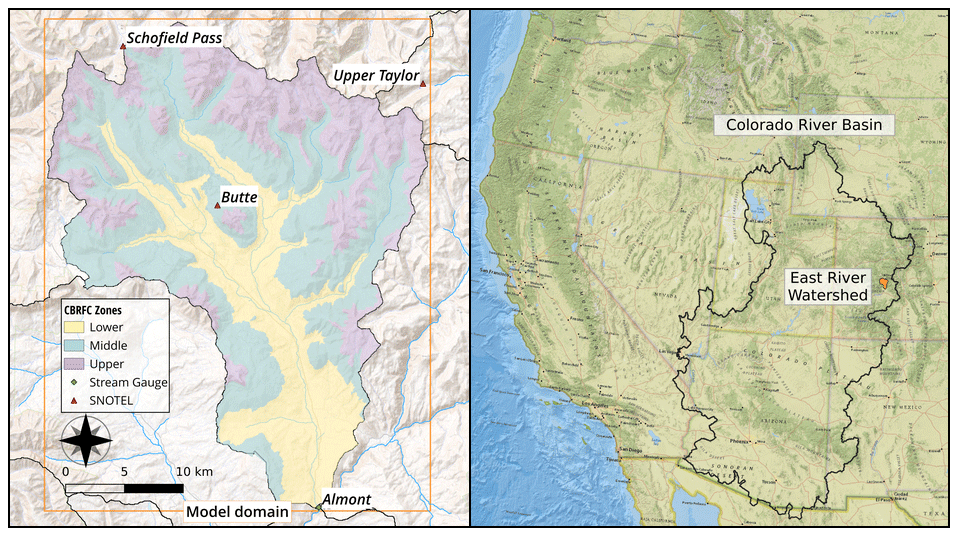
Figure 1Overviews of the East River Watershed (black boundaries) and iSnobal modal domain (orange outline) are shown on the left. There are three SNOTEL sites along with the stream gauge station. The watershed is divided into three HRUs by the CBRFC. The location of the watershed and area of the Colorado River Basin is shown on the right. Basemap (right): © ESRI.
The East River Watershed (ERW) is a high alpine watershed located in the Upper Gunnison River Basin, part of the Colorado River Basin. The East River is one of two primary tributaries of the Gunnison River, which discharges downstream into the Colorado River (Fig. 1). A stream gauge station at an elevation of 2440 m near Almont, Colorado, is operated by the United States Geological Survey (USGS) and monitors the streamflow of the East River year-round. This station is the central discharge point for seasonal snow runoff in the watershed. The ERW has representative characteristics for mountain watersheds in Colorado with an average elevation of 3266 m, a high vertical elevation relief (1420 m; Hubbard et al., 2018), and a mixture of different vegetation types (bush and grassland or mixed conifer and aspen trees).
There are three Snow Telemetry (SNOTEL) stations with available snow depth measurements that are operated by the United States Department of Agriculture National Resource Conservation Service (USDA-NRCS) in the modeled domain: Schofield Pass (elevation: 3261 m), Butte (elevation: 3097 m), and Upper Taylor (elevation: 3243 m). The Upper Taylor station does not sit within the ERW boundaries but was included in this study to expand the number of available in situ comparison sites within the model domain. The CBRFC divides the ERW into three topographical hydrologic response units (HRUs): lower, middle, and upper (Fig. 1). All HRUs are based on elevation (2896 m/9500 ft < middle < 3353 m/11 000 ft) and are modeled independently of each other (Council, 2006). The division will be used in this work to refer to the respective spatial area.
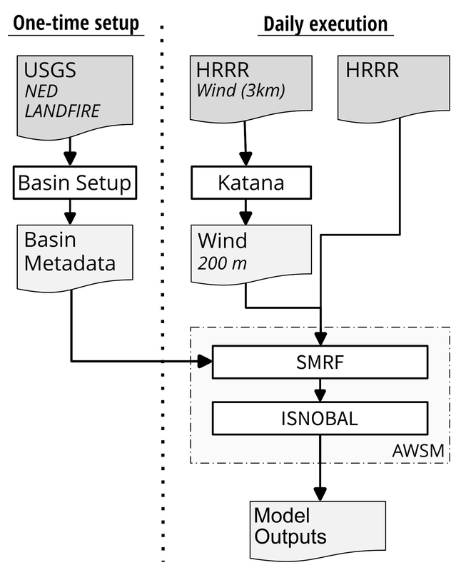
Figure 2Overview of the iSnobal model architecture showing the one-time setup process and the daily execution workflow.
3.1 Model architecture
A complete setup of the iSnobal model requires the installation of several components (Fig. 2). First, the “Basin Setup” tool (https://github.com/USDA-ARS-NWRC/basin_setup, last access: 28 February 2022) is installed, which assists in setting up the model domain boundaries, output resolution, and collecting the elevation and vegetation data. This one-time process is not repeated between simulation years and is stored in one central basin metadata file. Next, the daily execution components of the model are set up and consist of
-
Katana (https://github.com/USDA-ARS-NWRC/katana, last access: 28 February 2022),
-
SMRF (https://github.com/USDA-ARS-NWRC/smrf, last access: 28 February 2022), and
-
AWSM (https://github.com/USDA-ARS-NWRC/awsm, last access: 28 February 2022).
Katana is a pre-processing module that uses the WindNinja model (Forthofer et al., 2014) at its core to downscale the HRRR wind data to a higher resolution (e.g., from HRRR 3 km to 200 m). The SMRF module (Havens et al., 2017) develops the high-resolution hourly spatial forcing data required by iSnobal using coarser-resolution HRRR surface variables. AWSM (Havens et al., 2020) is the overarching control software that streamlines the execution for each time step and the iteration from one day to the next between SMRF and iSnobal.
All the above components were written and are maintained by the United States Department of Agriculture, Agriculture Research Service (USDA-ARS) in Boise, Idaho, USA. Each component is fully open-source software and installable from the source via GitHub (https://github.com, last access: 28 February 2022) or downloadable as a Docker container. A Docker container is a virtualized environment that combines the required operating system, libraries, and the application itself into one executable entity.
3.2 Model configuration
Each component of the model (Katana, SMRF, AWSM) is controlled by a configuration file that allows the user to customize parameters used during execution. For instance, when distributing forcing data from HRRR with SMRF, the user can change values for minimum and maximum air temperature, maximum and minimum snow grain sizes when calculating albedo decay, or the height above ground when calculating turbulent fluxes from the wind data. An overview of the possible options and default values for each component is available in the respective published documentation. For this application, no parameters were changed from the default values, and the configuration files are available on GitHub (https://github.com/UofU-Cryosphere/isnoda, last access: 28 February 2022).
3.3 East River Watershed model domain setup and execution
Elevation data at arcsec (approximately 10 m) resolution from the USGS National Elevation Dataset and 30 m vegetation data (height and type) from the USGS through the LANDFIRE spatial products were used as input for the Basin Setup tool. Both data sources are publicly available and distributed through the USGS (see the “Data availability” section). Basin Setup was further configured to prepare the ERW model domain at a 50 m spatial resolution, resulting in 837×656 grid cells and an area of 1373 km2. This spatial resolution was guided by the recommendations of Winstral et al. (2014), which found that iSnobal output resolutions of around 100 m kept the errors for SWE and surface water input (SWI) below ±5 % during the melt season compared to coarser resolutions. We further selected the 50 m resolution to keep the resampling of the vegetation data from LANDFIRE minimal and removed the need to interpolate the spatial snow depth product used in validation (Sect. 4). This resolution additionally better represents the terrain complexity, relevant for radiation calculations and interpolation of the HRRR-supplied forcing data within SMRF. Lastly, we also found that the 50 m resolution does not inhibit daily run times and scales for the operational requirements.
Snowpack mass and energy fluxes were simulated with iSnobal from 2018 through 2021 in 1 h time steps, matching the HRRR temporal resolution. The model was configured to store the end-of-day values (e.g., snow depth) or accumulated daily values (e.g., SWI), matching the temporal resolution of the available in situ comparison observations and the SNOW-17 inputs and outputs, which are further explained in the model comparison section. A single simulation year starts on 1 October and ends on 30 September. This date range is a “water year” and a standard definition for hydrologic forecasting in the United States.
3.4 Model forcing data
The meteorological inputs required to run the model were retrieved from the sixth-hour HRRR forecast product. HRRR is undergoing active development, and the water years simulated in this study used the product versions HRRRv2 (October 2017 to July 2018), HRRRv3 (July 2018 to November 2020), and HRRRv4 (December 2020 to August 2021). Using the sixth-hour HRRR forecast allows for better utilization of model physics along with the assimilated observations (Bytheway et al., 2017) and is a common practice for other NWP input products (Schirmer and Jamieson, 2015).
The required iSnobal forcing input data supplied from HRRR are air temperature, relative humidity, incoming shortwave radiation, wind speed and direction, and total precipitation. Using the wind data from HRRR (U and V component, 10 m above ground), Katana resolves the wind data to a 200 m resolution using the model domain elevation data. The 200 m resolution was a compromise between the iSnobal-simulated resolution (50 m) and the increased computational resources required by WindNinja to downscale from the 3 km HRRR grid.
3.5 iSnobal and SMRF description
Using temporally complete meteorological input data, the iSnobal model (Marks et al., 1999) simulates snowpack evolution by solving energy and mass balance fluxes. As a two-layer model, the top layer is designated for all energy and mass exchanges between the snow surface and the atmosphere. The bottom layer acts as an interface for mass and energy exchanges between the top and a single soil layer. At each simulated time step (1 h for the current application), the model calculates the snowpack net radiative, sensible, latent, conductive, and advective energy fluxes. Once the net energy fluxes of the two snow layers exceed the cold content (the energy required to raise the temperature across both layers to 0 ∘C) and the snow meltwater amount exceeds the maximum liquid water holding capacity of the snowpack, the water outflow of the snowpack is calculated and added to the SWI for that time step. At the end of a time step, the updated snowpack state variables (depth, density, temperature, and liquid water content) are stored and used as initialization values at the beginning of the next time step.
Before calculating the fluxes, the input data are spatially interpolated and distributed for the model domain in SMRF, which also prepares additional essential variables for the energy balance calculations in iSnobal. The variables include information for precipitation phase, precipitation temperature, percentage of snow in precipitation, and water vapor pressure. The required net shortwave radiation input used in iSnobal is calculated by SMRF from the topographically adjusted incoming clear-sky radiation (Dozier and Frew, 1990) and reduced with the percentage of cloud cover. The cloud cover itself is determined by the supplied incoming shortwave radiation from HRRR. An additional adjustment to the incident shortwave radiation reduces the value by vegetation type and height information from the vegetation metadata following Link and Marks (1999). The amount of reflected shortwave radiation is calculated using a simulated snow albedo derived with a time-decay function based on the time duration since the last snowfall. The difference between the cloud and vegetation-adjusted incident shortwave and the reflected shortwave results in the net shortwave radiation at the snow surface.
The net longwave radiation is calculated similarly to the net shortwave radiation in SMRF. First, the percentage of cloud cover is used to adjust the incoming longwave fluxes from a theoretical clear-sky atmosphere before the vegetation data are used to do a final correction (Link and Marks, 1999). From the downscaled wind data from the Katana module, SMRF interpolates the wind speeds to the configured output resolution. The SMRF options include the ability to account for precipitation redistribution using the speed and direction wind data according to Winstral and Marks (2002). However, this option was not used in this study and reduced potential error sources when comparing the HRRR precipitation input data to SNOW-17, which is explained in Sect. 4 below.
A detailed description of the energy balance equations and data preparation can be found in Marks et al. (1992, 1998, 1999), Link and Marks (1999), and Havens et al. (2017, 2020). All energy and mass balance calculations in iSnobal are based on a fixed spatial grid and a configurable time interval. The main driver for the chosen time interval to update the snowpack conditions is the temporal resolution of the input data, which needs to be fine enough to resolve diurnal climatic variations (e.g., temperature or shortwave radiation).
3.6 Model computing environment
The computational resources required for running the model in this work were provided by the Center for High Performance Computing at the University of Utah. All model components were installed from the source, with the exception of Katana, where the containerized option was selected due to the complexity of dependent libraries. The installation was documented and published on GitHub (https://github.com/UofU-Cryosphere/isnoda, last access: 28 February 2022) and extends the official documentation for each component with instructions for a shared compute environment and helper scripts for data download and model execution.
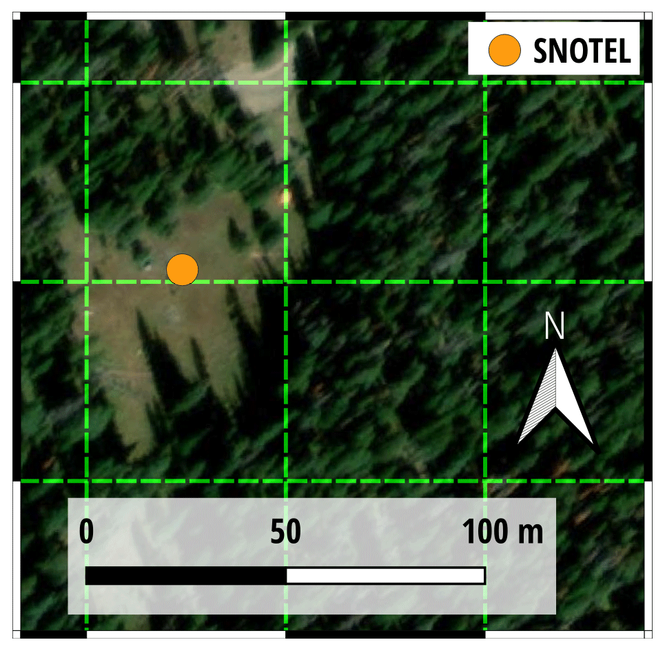
Figure 3SNOTEL Schofield Pass site location relative to the configured model output resolution of 50 m (green-dashed grid). No site was centered in one pixel, and a spatial 2×2 grid surrounding the site was used for simulated HRRR-iSnobal comparison values. Basemap: © ESRI.
Two types of measurements were used to compare selected iSnobal outputs with reference values: discrete in situ time-series measurements and spatially distributed snapshots at a single point in time. The in situ observations were the quality-controlled end-of-day values for snow depth measurements from the three SNOTEL stations. This assessment against the SNOTEL data used a spatial maximum and minimum of a 2×2 grid surrounding the point location of the sites (Fig. 3). This approach was based on visual inspections of the locations. Each site showed an offset to the center of the model output cell, and a spatial grid was deemed more appropriate to account for the physiographic variability surrounding their location. For the years with available Airborne Snow Observatory (ASO, Painter et al., 2016) aerial observations (2018 to 2020), simulated snow depths were compared to the ASO lidar-based snow depth products. The range of snow depth values on ASO flight days was also included in the in situ time-series comparison and used the same 2×2 grid surrounding the SNOTEL sites (Fig. 3).
The spatial point in time comparison used the snow depth maps from ASO, which surveyed the area twice in 2018 and 2019 and once in 2020. In 2018 and 2019, the first survey happened during the snow accumulation season, and the second survey happened after peak SWE during snowmelt progression. In 2020, the area was surveyed before peak SWE. The spatial resolution of the ASO snow depth maps matched the iSnobal model resolution of 50 m, and the spatial extent overlapped with the ERW boundaries. Across the years, the ASO snow depth maps were subtracted from the model-simulated snow depth on a pixel-by-pixel basis. Additionally, HRRR-iSnobal-simulated snow depths were compared to ASO snow depths in each HRU. The goal of this comparison was to check for any spatial biases in simulated snow depths across elevation bands or aspects and for different snow conditions (accumulating or melting) in years with two flights (2018 and 2019).
To assess how well HRRR-iSnobal compares to SNOW-17 for operational forecasting, the precipitation input and the outputs of SWE and SWI were compared. The data for SNOW-17 were supplied by the CBRFC. Mean areal SNOW-17 precipitation inputs originate from quality-controlled measurement stations in and around ERW and are combined using a weighting equation that is derived during calibration targeting PRISM (Parameter elevation Regression on Independent Slopes Model) statistical mapping grids. The comparison of precipitation and SWE used the CBRFC HRU division (Fig. 1) and summarized the iSnobal-HRRR data by the respective area. The SWI comparison also included the stream gauge discharge at the basin pour point and aggregated the model outputs within the watershed boundaries. This assessment used a 7 d moving average window to reduce daily spikes in the time series. The focus of this evaluation was on timing and magnitude; in a basin like ERW, the simulated SWI should follow the temporal pattern measured at the stream gauge, which is dominated by the snowmelt runoff (Carroll et al., 2018). Neither of the model outputs is considered the true value; rather, the intercomparison was undertaken to understand how (and why) the models may differ.
5.1 Run time
Running the model through an entire water year took around 18 h in total, with WindNinja taking one-third of the time and AWSM accounting for the remaining 12 h. The compute times are based on a machine with 24 processor cores, 24 GB of RAM, and hyper-threading enabled, which increased the number of processing threads to 48. The storage requirement for the input data was 10 GB, with the model output occupying another 100 GB of space. Iterating from one day to the next took less than 5 min, including data download, pre-processing, and running the model. This reasonably fast execution and total storage requirement showed that the model could be implemented in day-to-day operations.
5.2 Point comparison
For the two sites within the ERW boundaries (Butte and Schofield Pass), the simulated depths prior to peak snow depth had mean differences of 12 % to −16 % at Butte and 1 % to −21 % at Schofield Pass across the years. The Upper Taylor site had consistently higher than observed snow depth: 21 % to 37 %. The site-specific differences were not affected by annual differences in the snow accumulation magnitudes. Examples of an average snow depth year (2018) and an above-average year (2019) are shown in Fig. 4. Results for 2020 and 2021 are shown in Fig. S1 in the Supplement.
Table 1Overview of date differences for the last day with snow present between the HRRR-iSnobal and SNOTEL sites.

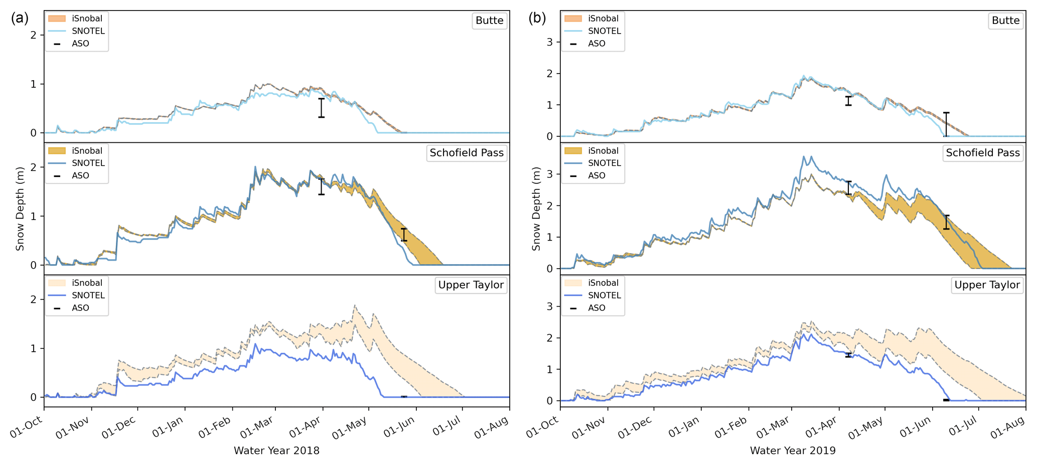
Figure 4Snow depth comparison between the HRRR-iSnobal and SNOTEL sites for the years 2018 (a) and 2019 (b). The orange-shaded areas represent the range of 2×2 grid cell values from HRRR-iSnobal surrounding the site. The ranges of the grid cell (50 m) values from ASO surveys are shown by the black bars. Note the different y scales between 2018 and 2019.
After the seasonal peak snow depth, simulated snow depths around all three SNOTEL stations deviated from observations, and the range of simulated values increased. Notably, the date for snow disappearance was simulated later with a varying difference in days relative to observations across all years. For instance, the difference between HRRR-iSnobal and all SNOTEL sites was between 11 and 59 d in 2018 and between −8 and 59 d in 2019. An overview of the differences between observations and simulation dates is shown in Table 1. Consequently, the percentage mean difference between HRRR-iSnobal and SNOTEL snow depths increased considerably, and values at the Butte site were between 27 % and −6 %. The Schofield Pass site mean differences ranged from 19 % to −46 % (−0.27 m). This disagreement in snowmelt rates and snow disappearance is further discussed in Sect. 6.4. An overview of the per-year and site differences is shown in Fig. S2, with mean differences given in Table S1. Overall, the snow depth comparison to observations over multiple years showed that the model can capture peak snow depth timing and magnitude.
A cross-comparison of snow depths on ASO flight days between the observed in situ SNOTEL sites, ASO remotely sensed values, and HRRR-iSnobal-simulated values showed a mixed result for agreement across the SNOTEL locations. At the Butte site, the early survey flights across all years had HRRR-iSnobal consistently higher than ASO. However, the measured values at this SNOTEL site agreed more with the 2×2 spatial grid snow depths of HRRR-iSnobal (difference ranging from −0.19 to +0.13 m for all years) versus ASO (−0.48 to −0.07 m). The 2018 late survey flight values agreed across all three sources for Butte, where snow was completely melted. In 2019, HRRR-iSnobal still had snow present, with ASO and SNOTEL showing complete meltout. Schofield Pass had good agreement across all snow depth values for the early 2018 flight (HRRR-iSnobal difference +/−0.04 m; ASO +0.05 m and −0.16 m), whereas the above-average 2019 season had lower values in HRRR-iSnobal with ASO capturing the SNOTEL depth value. The 2018 late survey flight had iSnobal-HRRR and ASO above the Schofield Pass value, with HRRR-iSnobal and ASO having a similar spatial range (HRRR-iSnobal: 0.34 m; ASO: 0.25 m). In 2019, the late survey flight captured the site value (1.50 m) in HRRR-iSnobal (range from 0.84 to 1.61 m) and ASO (1.25 to 1.68 m). The Upper Taylor site location was only included in the early 2019 flight and confirmed the strong overestimation by HRRR-iSnobal (1.61 to 2.06 m) as the ASO snow depth values (1.40 to 1.61 m) agreed with the SNOTEL depth (1.45 m). The agreement between ASO and SNOTEL and overestimation by HRRR-iSnobal was in both late survey flights for 2018 and 2019 at the Upper Taylor location, as the snow depths approached 0 m. An overview of snow depth values across all ASO flight years is given in Table S2. Overall, using ASO as an additional snow depth reference data set at discrete point locations in the model domain showed no consistent oversimulation or undersimulation for HRRR-iSnobal across the years.
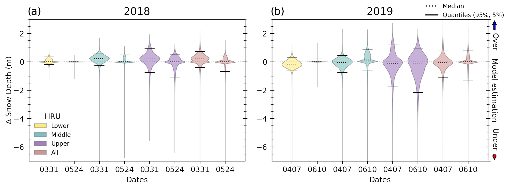
Figure 5Snow depth differences for early and late surveys for the years 2018 and 2019 between HRRR-iSnobal and ASO. Panels (a) and (b) categorize the differences by elevation HRU (low, middle, upper), with “All” showing the basin-wide difference.
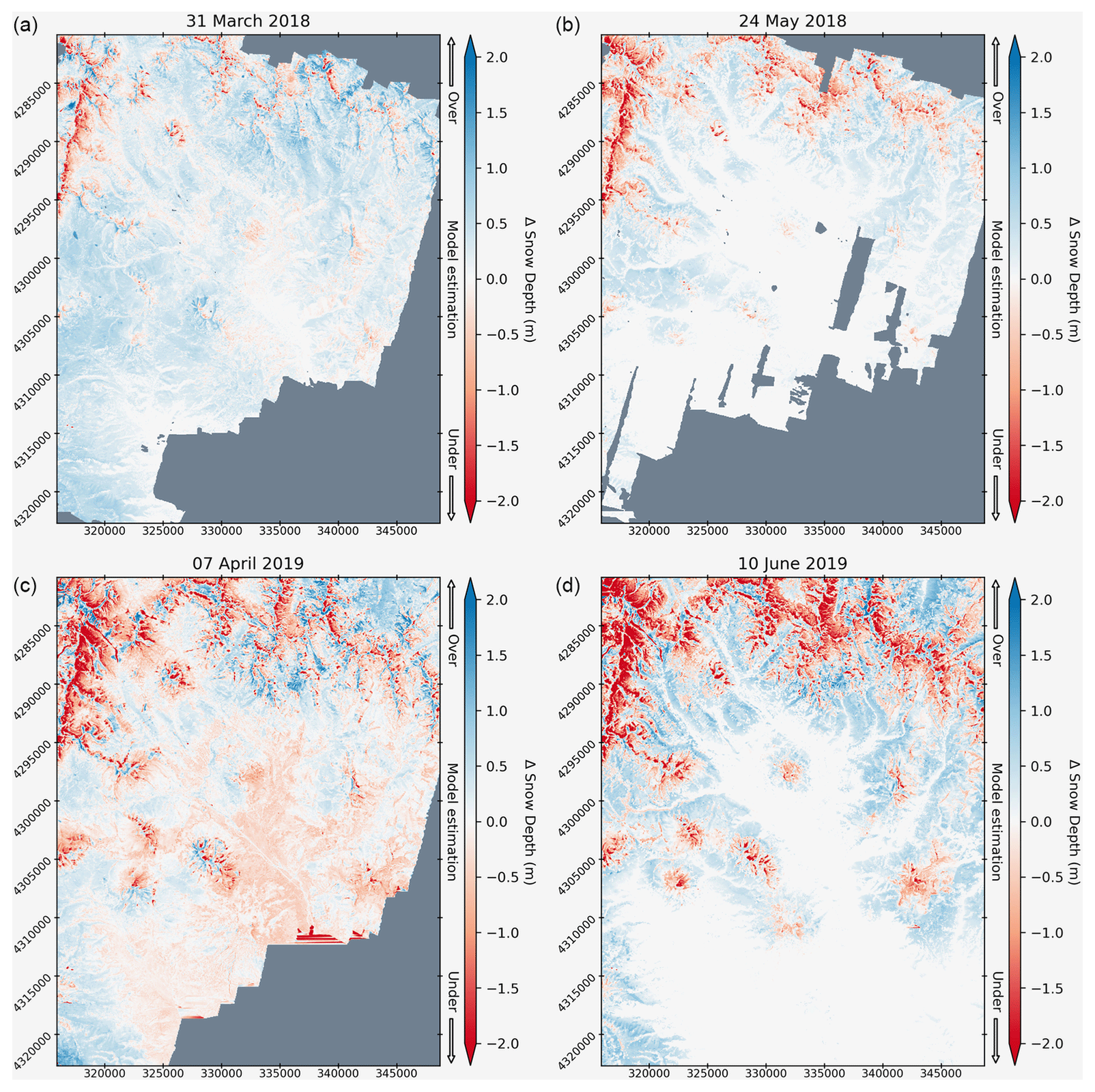
Figure 6Spatial comparison of simulated HRRR-iSnobal against observed ASO lidar-based snow depths for 2018 and 2019. Early surveys (a, c) and late surveys (b, d) subtracted ASO values per grid cell from HRRR-iSnobal (50 m resolution).
5.3 Spatial comparison
Integrated over the full basin, simulated snow depths agreed with ASO snow depths, with median differences of 0.20 m (early survey) and 0.00 m (late survey) in 2018, −0.06 m (early) and 0.00 m (late) in 2019, and 0.06 m in 2020. The distribution of the differences is shown with the “All” category in Fig. 5. Generally, between two flights in the same season, the agreement was best during late flights in the middle and lower HRU (Fig. 5a and b). An aerial overview with per-grid cell difference for the 2018 and 2019 flights is shown in Fig. 6, and 2020 can be found in Fig. S3. Within lower, middle, and upper HRU elevations, the widest range in the Δ snow depth distribution was consistently found at the upper HRU (standard deviation (SD) between 0.53 and 0.99 m across the flights), while the lower HRU (SD 0.03 to 0.55 m) and middle HRU showed similar ranges (SD 0.22 to 0.53 m). The distributions of Δ snow depth for the late survey in each year showed positive biases, indicating a general overestimation of snow depths by HRRR-iSnobal, consistent with the observed slower snow depth decrease during the snowmelt season at the SNOTEL sites (Fig. 4).
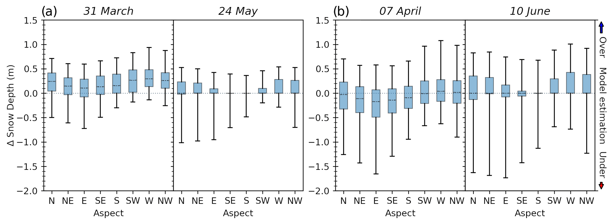
Figure 7Snow depth differences for the water years 2018 (a) and 2019 (b) between ASO and HRRR-iSnobal binned by aspect.
The snow depth differences binned by aspect for the entire watershed indicated a bias, with variation during flight dates and the two years (Fig. 7a and b). In both early flights, higher snow depth was measured on eastern aspects relative to other aspects, and the widest ranges in snow depth differences were on northern aspects in both late flights. The closest agreement between modeled and ASO snow depths was on the east- to south-facing slopes during late flights, as most snow was melted at that time of the season.
Table 2Overview of precipitation inputs and SWE outputs for HRRR-iSnobal and SNOW-17 classified by HRU.

Note: precipitation (Precip.) and SWE values are shown in millimeters.
5.4 SNOW-17 comparison
Generally, precipitation used as an input to SNOW-17 was consistently higher than the HRRR precipitation input used for iSnobal across all years. The difference ranged from HRRR being 25 % (2021) to 5 % (2018) lower, integrated across all HRUs. A summary of the comparison, per HRU and for the full watershed, is in Table 2. Using SNOW-17 as the reference, the daily total amount difference was consistent across the HRUs and years, with no high ratio differences (Fig. S4). For total amounts per HRU, the poorest agreement was in the lower HRU in 2020, with HRRR 36 % lower. The best agreement was found in the middle HRU in 2018, with a match of 99 %. The differences per HRU were not correlated with whether it was a high or low snow year, with similar agreement in 2018 (lowest snow) and 2019 (highest snow). The poorest overall agreement (2020 and 2021) had a higher precipitation amount for SNOW-17 (2020: 18 %, 2021: 25 %), which was not reflected in the SNOTEL site comparison. The snow depth across all sites in 2020 had a mean difference between −0.20 and +0.23 m and between −0.17 and +0.02 m in 2021 in the pre-melt season (Fig. S2). Both of the years had similar HRRR total precipitation amounts compared to 2018 (differences 2020: −64 mm, 2021: −66 mm), which is also supported by the similar depth at all SNOTEL sites to 2018 (Fig. S1).
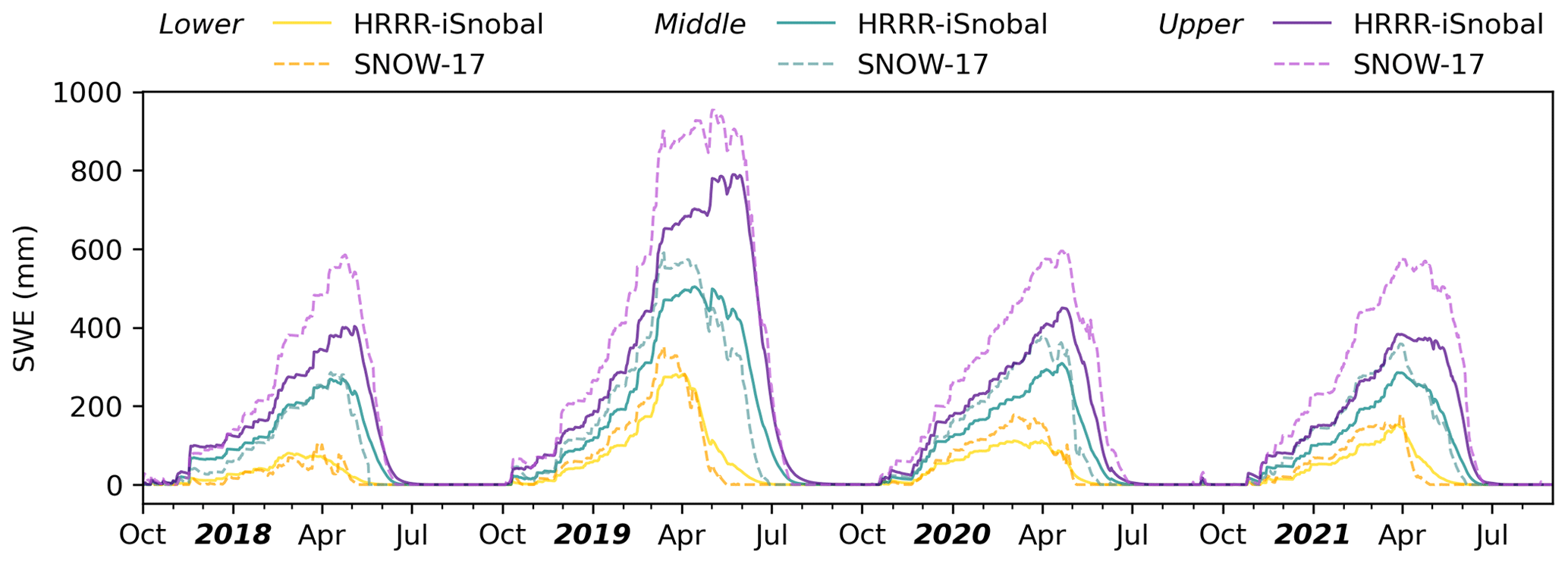
Figure 8Total SWE comparison per HRU across 4 years between SNOW-17 (dashed lines) and HRRR-iSnobal (solid lines).
Across the four years, all three HRUs showed similar temporal patterns for daily total SWE in the snowpack, although HRRR-iSnobal SWE was lower in magnitude (Fig. 8) and expected following the precipitation comparison (Table 2). Consequently, the largest difference between the two models was in the upper HRU (HRRR-iSnobal between −34 % and −20 %), with less difference in the middle (HRRR-iSnobal between +20 % and −15 %) and lower (HRRR-iSnobal between +25 % and −23 %) HRUs. As with the SNOTEL depth comparison, the basin SWE from HRRR-iSnobal showed longer persistence of snow compared to SNOW-17. This lag is most apparent in the lower and middle HRU, with the upper HRU having similar SWE depletion timing.
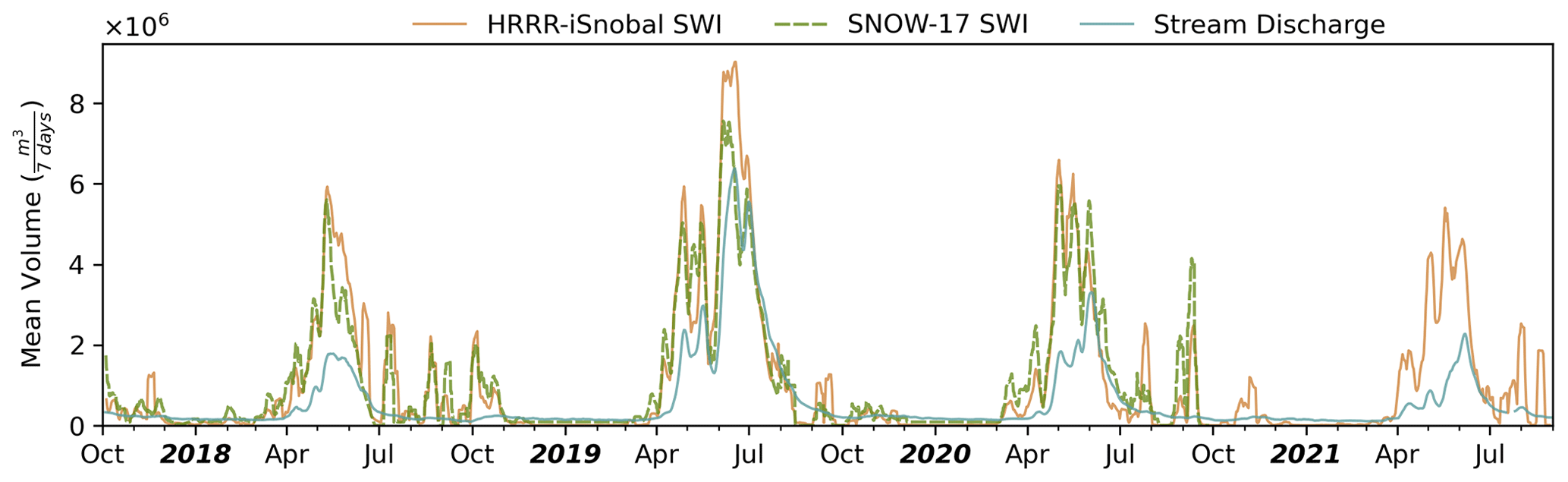
Figure 9Time series comparison of simulated HRRR-iSnobal SWI and SNOW-17 SWI against the measured USGS stream gauge discharge across the 4 water years. Note: the data for SNOW-17 SWI were not available for 2021.
The watershed 7 d moving average of simulated HRRR-iSnobal SWI compared to SNOW-17 matched the SWI timing of the first peak at the beginning of every melt season (Fig. 9). Afterwards, the SNOW-17 mean volume was lower, with HRRR-iSnobal showing more water outflow. This difference in magnitude can in part be explained by the difference in SWE, where HRRR-iSnobal SWE persisted longer into the melt season, with SNOW-17 depleting earlier (Fig. 8). Compared to the stream gauge, HRRR-iSnobal followed the hydrograph timing and magnitude pattern across the years. During the annual snowmelt pulse, HRRR-iSnobal stayed higher relative to the discharge at the gauge. This higher peak was expected, as a portion of SWI is taken up by the ground, plants, and atmosphere before reaching the gauge. In summary, the general patterns and magnitude of HRRR-iSnobal SWI showed no underforecasting at any point in the melt season when compared to simulated SNOW-17 SWI and measured stream gauge discharge.
6.1 HRRR precipitation
The results for the snow depth comparison to SNOTEL and ASO indicated that the HRRR precipitation allowed iSnobal to simulate the snow mass balance well. This is promising because HRRR data are distributed at 3 km resolution and are much coarser than the 50 m model output resolution, which is needed to resolve the different physical processes influencing the snowpack evolution in this type of terrain (Winstral et al., 2014). The difference in resolutions makes it challenging to properly adjust for the topographic precipitation differences, especially with the model domain's high vertical relief (1420 m). Kilometer-scale NWP model resolutions are known to underestimate snowfall at higher elevations, and complex terrain is particularly challenging for simulating snowpack evolution with inconsistent snowfall trends (Ikeda et al., 2010). The current solutions to “bias-correct” and improve NWP precipitation based on topography are basin- and application-specific. For example, Bellaire et al. (2011, 2013) applied a constant correction factor, and Griessinger et al. (2019) corrected and filtered with observations from a dense in situ network. These approaches require in situ observation and basin-specific knowledge that is not always available, reducing transferability to other regions. Ultimately, the fewer corrections needed for forcing inputs results in greater potential to scale and adapt model setups into forecast operations. The presented workflow here had no changes to the HRRR inputs, and precipitation was used “as is”.
Given the different methods to determine precipitation in HRRR and as inputs to SNOW-17, a match between the two was not expected. The calibration process for SNOW-17 precipitation inputs uses spatially sparse in situ point measurements and empirical data from previous water years. As an atmospheric model, HRRR is a product of assimilated observation, physically based modeling, and a fundamentally different approach. Neither set of precipitation values was considered the truth, and accurately measuring precipitation is an unsolved challenge in mountain terrain. Additional work is needed to understand the variation in HRRR values relative to the calibrated precipitation used by the CBRFC across these water years (i.e., poorer agreement in 2020 and 2021).
6.2 Comparison data sources
The snow depth comparison of this work used in situ point observations and aerial spatial measurements. Both sources had no consistent agreement, with the spatial measurements tending to be lower than the point data. This underestimation has been shown to exist when comparing point data to spatial averages of snow depth from lidar (Trujillo and Lehning, 2015). Similarly, in situ snow depth estimates from point observation stations, such as SNOTEL, are known to only represent a small surrounding footprint because of the large heterogeneity of snow depth in alpine environments (Molotch and Bales, 2005). This limitation, in part, can explain the higher spread of the iSnobal snow depths to the SNOTEL stations, as the values represent a larger area around them (Fig. 3). The strength of SNOTEL station data is as long-term historical records, from which index methods could be developed and help understand changes over long timeframes (Harpold et al., 2012; Musselman et al., 2021; Trujillo and Molotch, 2014). In the case of this work, it was the only source available to allow a model performance assessment over multiple years. The results from the SNOTEL comparison gave confidence that the HRRR forcing inputs provided a quality long-term input source, in terms of capturing peak snow depth, for a watershed with only sparse in situ meteorological observations across different snow seasons.
The addition of aerial observations, such as ASO, has improved the ability to retrieve snow depth over large areas and supplies valuable validation data used in many studies (Brandt et al., 2020; Hedrick et al., 2018; McGrath et al., 2019). In this work, the ASO maps enabled a spatial comparison that was impossible in the past. The comparison identified differences in snow depth at high elevations and across aspects that are not possible with SNOTEL stations, which are generally located at relatively flat middle and lower elevations (e.g., below 3261 m in ERW). Additionally, the snow depth disagreements between measured ASO and SNOTEL highlighted that SNOTEL observations could not represent snow conditions at 50 m model output resolutions either, and caution is urged when using SNOTEL snow depth data as “truth” for spatially distributed models. Likewise, the inconsistent comparison results to SNOTEL showed that coarser aerial product resolutions should also not be treated as truth, and snow depths can vary within short distances due to the high spatial variability of mountain terrain.
6.3 Physically based models
Accurately simulating the seasonal snow accumulation and depletion across multiple years and different topographic regions through a single model is still an unsolved challenge. However, physically based models are better suited to fulfilling this need when compared to temperature-index-based models. Existing studies using long-term records of SNOTEL measurements have identified a need for physically based modeling approaches as they can better show the impacts on water supply from current and projected climatological changes (Harpold et al., 2012; Musselman et al., 2021; Trujillo and Molotch, 2014). Physically based models are capable of accounting for scenarios such as shifting snowmelt rates (Musselman et al., 2017), changes to the length of snow accumulation and melt season (Trujillo and Molotch, 2014), accelerated melt due to darker snow (Skiles and Painter, 2019), and rain-on-snow events (Marks et al., 1998).
The HRRR-iSnobal combination in this work closely simulated the snow depth observations from one region across different seasonal characteristics (average vs. non-average year) without a priori region-specific knowledge. All required forcing data per water year only used the HRRR-forecasted observations of that year, replacing the sparse in situ measurements that are interpolated and calibrated with historical data. The interpolation and calibration procedures are essential steps in the current SNOW-17 workflow of the CBRFC and require regional forecaster experience. Voiding this need gives a major operational advantage by simplifying model application and enhancing the ability to adapt to environmental changes across different regions and water years.
In addition to the streamlined forcing data preparation, the advantages during the water year simulation include the replacement of region-specific parameters required by temperature-index models (e.g., the SNOW-17 melt factor) with the energy balance calculations from physically based models. The index model parameters depend again on forecaster experience and require forecaster changes in response to changing environmental conditions (average vs. non-average). In this work, there was no need to change the model configuration between the 2018 (average) and 2019 (above-average) years in HRRR-iSnobal. The seasonal differences were accounted for explicitly as the snow energy balance calculations include influences such as shortwave radiation (Marks and Dozier, 1992), longwave radiation (Link and Marks, 1999), and turbulent fluxes from terrain-dependent wind speeds (Winstral and Marks, 2002). Lastly, iSnobal is a spatially distributed model run with a user-defined output resolution (50 m in this study) and set up with site-specific elevation and vegetation data information from the model domain. This configuration negated the need to divide the model domain into uniform and simplified HRUs to simulate the topographic differences of the model domain accurately.
In summary, physically based models remove the dependence on long-term historical calibration data, reduce the need for user intervention due to parametrization issues, require less model domain specific user knowledge, and better represent physiographic influences. All these factors combined result in improved scalability across different seasonal and terrain-dependent snowpack dynamics. Gradually adding these models into operational settings, with architectures presented in this work, can enhance snowpack information in response to current environmental perturbations and expand the ability to adapt to current and future water supply forecast needs.
6.4 Improvements to iSnobal
The consistent longer presence of snow in HRRR-iSnobal relative to the observations across the simulated years highlighted an area for improvement. One cause of the delay is attributed to the too low amount of calculated shortwave radiation by SMRF not providing enough energy to drive snowmelt in iSnobal. An obvious option that influences the calculation is the snow albedo time-decay function, which has caused high uncertainty in many different model types and scales (Chen et al., 2014; Clark et al., 2015; Krinner et al., 2018; Qu and Hall, 2014; Ryken et al., 2020). The decay function determines the snow albedo based on the time of the last snowfall when the albedo gets reset, and the decay starts anew. A drawback of this approach is excluding other events that change the albedo, such as dust deposition. Solutions for the 1-dimensional iSnobal model improved the simulated snowmelt timing and forced the model with observed snow albedo (Miller et al., 2016; Skiles and Painter, 2019; Skiles et al., 2015, 2012). Scaling this solution and adapting it into spatially distributed models requires data sources with daily updated and spatially complete snow albedo, which are available today from remote sensing observations. For instance, the combined Moderate-Resolution Imaging Spectroradiometer (MODIS) Snow Covered Area and Grain Size (MODSCAG) and Dust Radiative Forcing (MODDRFS) in Snow (Rittger et al., 2020) provides daily observation with 500 m spatial resolution. This spatial and temporal resolution fulfills the requirements of a model data source. With the demonstrated need for improved snow disappearance dates of this work, improved results by using observations in other work, and the availability of remote sensing products, we suggest integrating remotely sensed snow albedo into iSnobal.
Though relatively sparse in time, the spatial snow depth comparison results highlighted another area to target with HRRR-iSnobal. The snow depth differences by aspect (Fig. 5c and d) indicated an iSnobal energy balance issue as there was no strong aspect bias coming from the HRRR precipitation data (Fig. S5). This difference could also be caused by the disabled feature to account for wind redistribution. However, the closer agreements on the south-facing aspect, especially in the late survey ASO surveys, suggest that improving the incoming shortwave radiation could help address this model bias. Shortwave radiation is currently a topographically adjusted calculation (Dozier and Frew, 1990) by SMRF when preparing iSnobal forcing inputs. One alternative to this approach is to use the supplied values by HRRR, reducing model complexity and computation times. The addition of remotely sensed albedo and alternative handling for incoming shortwave radiation will be the follow-up effort for iSnobal to this work.
This work presented and evaluated the spatially distributed iSnobal model forced with HRRR meteorological data to expand the model options and support operational water forecasts for the CBRFC. The model was assessed over one representative headwater basin in the CRB with an area of 1373 km2 for 4 consecutive water years (2018 to 2021) at a 50 m spatial resolution and hourly time steps. There were several key outcomes from this effort. (1) Execution times from one to the next day and total storage requirements would allow operational forecasters to run HRRR-iSnobal alongside current production environments. (2) HRRR provided meteorological input data that enabled iSnobal to simulate close to the observed snow depths up to peak accumulation. (3) iSnobal radiation calculations need revisions to improve melt timing and to address geographic aspect bias. (4) Simulated timing and magnitude of iSnobal SWI followed the observed hydrograph at the basin stream gauge.
From the model comparison, the iSnobal SWE was lower than the SNOW-17 SWE and consistent with the lower precipitation inputs from HRRR than the SNOW-17 inputs. iSnobal had lower snow depths at higher elevations relative to aerial observations and was attributed to the coarser model output resolution of HRRR relative to the topography and the simulated spatial resolution. Model runs in additional basins are ongoing and will allow further evaluation if this is consistent. Despite these differences, iSnobal simulated snow depths close to measured values across the watershed up to the melt period. Once snowmelt set in, iSnobal snow depths showed greater disagreement than the observed in situ measurement sites and simulated longer snow persistence. The discrepancy between observed and simulated snowmelt timing, and therefore magnitude, was consistent across the years, including above-average and below-average snow years. Accurately simulating snow depletion timing is important for operational adoption. Future work to address snowmelt timing aims to improve snow energy balance calculations, specifically by using remotely observed snow albedo data and updating the net shortwave radiation treatment in iSnobal. Nevertheless, as the world transitions into a future that is less similar to the past and statistical models become less reliable, this work showed that HRRR-iSnobal could be a valuable supplement to operational water supply forecasting methods in snow-dominated regions.
The software components used to run the model and analyze the results are publicly available. iSnobal model components are available via the USDA ARS NWRC GitHub page: https://github.com/USDA-ARS-NWRC (last access: 28 February 2022). For this study, GitHub forks for SMRF (https://doi.org/10.5281/zenodo.6543935; Havens et al., 2022a), AWSM (https://doi.org/10.5281/zenodo.6543919; Havens et al., 2022b), and weather forecast retrieval (https://doi.org/10.5281/zenodo.6543579; Havens et al., 2022c) were created to capture the model code at the time of completing this study as no official version was released. The forks can be found under https://github.com/UofU-Cryosphere (last access: 28 February 2022). Additions to model setup and result analysis code are stored on https://doi.org/10.5281/zenodo.7452230 (Meyer and Ragar, 2022).
The following data sets were used for the model runs and comparisons.
-
https://apps.nationalmap.gov/viewer/ (last access: 28 February 2022; The National Elevation Dataset, 2022)
-
https://landfire.gov/getdata.php (last access: 28 February 2022; LANDFIRE, 2014)
-
https://rapidrefresh.noaa.gov/hrrr/ (last access: 28 February 2022; NOAA, 2022)
-
https://www.wcc.nrcs.usda.gov/snow/SNOTEL-wedata.html (last access: 28 February 2022; NRCS National Water and Climate Center, 2022).
-
https://www.usgs.gov/programs/national-geospatial-program/national-map (last access: 28 February 2022; U.S. Geological Survey, 2022a)
-
https://waterdata.usgs.gov/nwis/dvstat/?site_no=09112500&referred_module=sw&format=sites_selection_links (last access: 28 February 2022; U.S. Geological Survey, 2022b)
-
https://doi.org/10.5067/STOT5I0U1WVI (Painter, 2018)
The supplement related to this article is available online at: https://doi.org/10.5194/gmd-16-233-2023-supplement.
JM and SMS conceptualized the overall study, with helpful contributions from all the authors. JM performed the model runs and analysis. PK provided CBRFC data and support. SMS provided financial support for the study. JM wrote the first draft of the manuscript, which was then contributed to by all the authors.
The contact author has declared that none of the authors has any competing interests.
The USDA is an equal opportunity provider and employer.
Publisher's note: Copernicus Publications remains neutral with regard to jurisdictional claims in published maps and institutional affiliations.
The authors would like to thank Fabien Maussion, Bertrand Cluzet, and one anonymous referee for their helpful feedback and suggestions. The support and resources from the Center for High Performance Computing (CHPC) at the University of Utah are gratefully acknowledged.
This research has been supported by the NASA Earth Science Division Applied Sciences – Water Resources Program (grant no. 80NSSC19K1243).
This paper was edited by Fabien Maussion and reviewed by Bertrand Cluzet and one anonymous referee.
Anderson, E. A.: A point energy and mass balance model of a snow cover, United States, National Weather Service, https://repository.library.noaa.gov/view/noaa/6392 (last access: 28 February 2022), 1976.
Ayers, J., Ficklin, D. L., Stewart, I. T., and Strunk, M.: Comparison of CMIP3 and CMIP5 projected hydrologic conditions over the Upper Colorado River Basin, Int. J. Climatol., 36, 3807–3818, https://doi.org/10.1002/joc.4594, 2016.
Bellaire, S., Jamieson, J. B., and Fierz, C.: Forcing the snow-cover model SNOWPACK with forecasted weather data, The Cryosphere, 5, 1115–1125, https://doi.org/10.5194/tc-5-1115-2011, 2011.
Bellaire, S., Jamieson, J. B., and Fierz, C.: Corrigendum to “Forcing the snow-cover model SNOWPACK with forecasted weather data” published in The Cryosphere, 5, 1115–1125, 2011, The Cryosphere, 7, 511–513, https://doi.org/10.5194/tc-7-511-2013, 2013.
Benjamin, S. G., Weygandt, S. S., Brown, J. M., Hu, M., Alexander, C. R., Smirnova, T. G., Olson, J. B., James, E. P., Dowell, D. C., Grell, G. A., Lin, H., Peckham, S. E., Smith, T. L., Moninger, W. R., Kenyon, J. S., and Manikin, G. S.: A North American Hourly Assimilation and Model Forecast Cycle: The Rapid Refresh, Mon. Weather Rev., 144, 1669–1694, https://doi.org/10.1175/MWR-D-15-0242.1, 2016.
Brandt, W. T., Bormann, K. J., Cannon, F., Deems, J. S., Painter, T. H., Steinhoff, D. F., and Dozier, J.: Quantifying the Spatial Variability of a Snowstorm Using Differential Airborne Lidar, Water Resour. Res., 56, https://doi.org/10.1029/2019WR025331, 2020.
Bryant, A. C., Painter, T. H., Deems, J. S., and Bender, S. M.: Impact of dust radiative forcing in snow on accuracy of operational runoff prediction in the Upper Colorado River Basin: DUST IN SNOW IMPACT ON STREAMFLOW, Geophys. Res. Lett., 40, 3945–3949, https://doi.org/10.1002/grl.50773, 2013.
Bytheway, J. L., Kummerow, C. D., and Alexander, C.: A Features-Based Assessment of the Evolution of Warm Season Precipitation Forecasts from the HRRR Model over Three Years of Development, Weather Forecast., 32, 1841–1856, https://doi.org/10.1175/WAF-D-17-0050.1, 2017.
Carroll, R. W. H., Bearup, L. A., Brown, W., Dong, W., Bill, M., and Willlams, K. H.: Factors controlling seasonal groundwater and solute flux from snow-dominated basins, Hydrol. Process., 32, 2187–2202, https://doi.org/10.1002/hyp.13151, 2018.
Chen, F., Barlage, M., Tewari, M., Rasmussen, R., Jin, J., Lettenmaier, D., Livneh, B., Lin, C., Miguez-Macho, G., Niu, G.-Y., Wen, L., and Yang, Z.-L.: Modeling seasonal snowpack evolution in the complex terrain and forested Colorado Headwaters region: A model intercomparison study, J. Geophys. Res.-Atmos., 119, 13795–13819, https://doi.org/10.1002/2014JD022167, 2014.
Cho, E., McCrary, R. R., and Jacobs, J. M.: Future Changes in Snowpack, Snowmelt, and Runoff Potential Extremes Over North America, Geophys. Res. Lett., 48, e2021GL094985, https://doi.org/10.1029/2021GL094985, 2021.
Christensen, N. S. and Lettenmaier, D. P.: A multimodel ensemble approach to assessment of climate change impacts on the hydrology and water resources of the Colorado River Basin, Hydrol. Earth Syst. Sci., 11, 1417–1434, https://doi.org/10.5194/hess-11-1417-2007, 2007.
Clark, M. P., Nijssen, B., Lundquist, J. D., Kavetski, D., Rupp, D. E., Woods, R. A., Freer, J. E., Gutmann, E. D., Wood, A. W., Gochis, D. J., Rasmussen, R. M., Tarboton, D. G., Mahat, V., Flerchinger, G. N., and Marks, D. G.: A unified approach for process-based hydrologic modeling: 2. Model implementation and case studies, Water Resour. Res., 51, 2515–2542, https://doi.org/10.1002/2015WR017200, 2015.
Council, N. R.: Toward a new advanced hydrologic prediction service (AHPS), The National Academies Press, Washington, D.C., 84 pp., https://doi.org/10.17226/11598, 2006.
Dettinger, M., Udall, B., and Georgakakos, A.: Western water and climate change, Ecol. Appl., 25, 2069–2093, https://doi.org/10.1890/15-0938.1, 2015.
Dozier, J. and Frew, J.: Rapid calculation of terrain parameters for radiation modeling from digital elevation data, IEEE T. Geosci. Remote, 28, 963–969, https://doi.org/10.1109/36.58986, 1990.
Essery, R.: A factorial snowpack model (FSM 1.0), Geosci. Model Dev., 8, 3867–3876, https://doi.org/10.5194/gmd-8-3867-2015, 2015.
Feng, S. and Hu, Q.: Changes in winter snowfall/precipitation ratio in the contiguous United States, J. Geophys. Res.-Atmos., 112, https://doi.org/10.1029/2007JD008397, 2007.
Forthofer, J. M., Butler, B. W., Wagenbrenner, N. S., Forthofer, J. M., Butler, B. W., and Wagenbrenner, N. S.: A comparison of three approaches for simulating fine-scale surface winds in support of wildland fire management. Part I. Model formulation and comparison against measurements, Int. J. Wildland Fire, 23, 969–981, https://doi.org/10.1071/WF12089, 2014.
Franz, K. J., Hogue, T. S., and Sorooshian, S.: Operational snow modeling: Addressing the challenges of an energy balance model for National Weather Service forecasts, J. Hydrol., 360, 48–66, https://doi.org/10.1016/j.jhydrol.2008.07.013, 2008.
Franz, K. J., Butcher, P., and Ajami, N. K.: Addressing snow model uncertainty for hydrologic prediction, Adv. Water Resour., 33, 820–832, https://doi.org/10.1016/j.advwatres.2010.05.004, 2010.
Garen, D. C. and Marks, D.: Spatially distributed energy balance snowmelt modelling in a mountainous river basin: estimation of meteorological inputs and verification of model results, J. Hydrol., 315, 126–153, https://doi.org/10.1016/j.jhydrol.2005.03.026, 2005.
Gowan, T. A., Horel, J. D., Jacques, A. A., and Kovac, A.: Using Cloud Computing to Analyze Model Output Archived in Zarr Format, J. Atmos. Ocean. Tech., 39, 449–462, https://doi.org/10.1175/JTECH-D-21-0106.1, 2022.
Griessinger, N., Schirmer, M., Helbig, N., Winstral, A., Michel, A., and Jonas, T.: Implications of observation-enhanced energy-balance snowmelt simulations for runoff modeling of Alpine catchments, Adv. Water Resour., 133, 103410, https://doi.org/10.1016/j.advwatres.2019.103410, 2019.
Harpold, A., Brooks, P., Rajagopal, S., Heidbuchel, I., Jardine, A., and Stielstra, C.: Changes in snowpack accumulation and ablation in the intermountain west, Water Resour. Res., 48, https://doi.org/10.1029/2012WR011949, 2012.
Havens, S., Marks, D., Kormos, P., and Hedrick, A.: Spatial Modeling for Resources Framework (SMRF): A modular framework for developing spatial forcing data for snow modeling in mountain basins, Comput. Geosci., 109, 295–304, https://doi.org/10.1016/j.cageo.2017.08.016, 2017.
Havens, S., Marks, D., FitzGerald, K., Masarik, M., Flores, A. N., Kormos, P., and Hedrick, A.: Approximating Input Data to a Snowmelt Model Using Weather Research and Forecasting Model Outputs in Lieu of Meteorological Measurements, J. Hydrometeorol., 20, 847–862, https://doi.org/10.1175/JHM-D-18-0146.1, 2019.
Havens, S., Marks, D., Sandusky, M., Hedrick, A., Johnson, M., Robertson, M., and Trujillo, E.: Automated Water Supply Model (AWSM): Streamlining and standardizing application of a physically based snow model for water resources and reproducible science, Comput. Geosci., 144, 104571, https://doi.org/10.1016/j.cageo.2020.104571, 2020.
Havens, S., Marks, D., Kormos, P., Hedrick, A., Trujillo, E., Johnson, M., Sandusky, M., and Robertson, M.: Spatial Modeling for Resources Framework (SMRF) (v0.9.1), Zenodo [code], https://doi.org/10.5281/zenodo.6543935, 2022a.
Havens, S., Marks, D., Sandusky, M., Johnson, M., Robertson, M., Hedrick, A., and Kormos, P.: Automated Water Supply Model (AWSM) (v0.10.0), Zenodo [code], https://doi.org/10.5281/zenodo.6543919, 2022b.
Havens, S., Meyer, J., Sandusky, M., Johnson, M., and Robertson, M.: UofU-Cryosphere/weather_forecast_retrieval: GMD submission (Version 20220512), Zenodo [code], https://doi.org/10.5281/zenodo.6543579, 2022c.
He, M., Hogue, T. S., Franz, K. J., Margulis, S. A., and Vrugt, J. A.: Characterizing parameter sensitivity and uncertainty for a snow model across hydroclimatic regimes, Adv. Water Resour., 34, 114–127, https://doi.org/10.1016/j.advwatres.2010.10.002, 2011.
Hedrick, A. R., Marks, D., Havens, S., Robertson, M., Johnson, M., Sandusky, M., Marshall, H., Kormos, P. R., Bormann, K. J., and Painter, T. H.: Direct Insertion of NASA Airborne Snow Observatory-Derived Snow Depth Time Series Into the iSnobal Energy Balance Snow Model, Water Resour. Res., 54, 8045–8063, https://doi.org/10.1029/2018WR023190, 2018.
Hedrick, A. R., Marks, D., Marshall, H., McNamara, J., Havens, S., Trujillo, E., Sandusky, M., Robertson, M., Johnson, M., Bormann, K. J., and Painter, T. H.: From Drought to Flood: A Water Balance Analysis of the Tuolumne River Basin during Extreme Conditions (2015–2017), Hydrol. Process., hyp.13749, https://doi.org/10.1002/hyp.13749, 2020.
Hubbard, S. S., Williams, K. H., Agarwal, D., Banfield, J., Beller, H., Bouskill, N., Brodie, E., Carroll, R., Dafflon, B., Dwivedi, D., Falco, N., Faybishenko, B., Maxwell, R., Nico, P., Steefel, C., Steltzer, H., Tokunaga, T., Tran, P. A., Wainwright, H., and Varadharajan, C.: The East River, Colorado, Watershed: A Mountainous Community Testbed for Improving Predictive Understanding of Multiscale Hydrological–Biogeochemical Dynamics, Vadose Zone J., 17, 0, https://doi.org/10.2136/vzj2018.03.0061, 2018.
Ikeda, K., Rasmussen, R., Liu, C., Gochis, D., Yates, D., Chen, F., Tewari, M., Barlage, M., Dudhia, J., Miller, K., Arsenault, K., Grubišić, V., Thompson, G., and Guttman, E.: Simulation of seasonal snowfall over Colorado, Atmos. Res., 97, 462–477, https://doi.org/10.1016/j.atmosres.2010.04.010, 2010.
Ikeda, K., Rasmussen, R., Liu, C., Newman, A., Chen, F., Barlage, M., Gutmann, E., Dudhia, J., Dai, A., Luce, C., and Musselman, K.: Snowfall and snowpack in the Western U.S. as captured by convection permitting climate simulations: current climate and pseudo global warming future climate, Clim. Dynam., 57, 2191–2215, https://doi.org/10.1007/s00382-021-05805-w, 2021.
Iwamoto, K., Yamaguchi, S., Nakai, S., and Sato, A.: Forecasting Experiments Using the Regional Meteorological Model and the Numerical Snow Cover Model in the Snow Disaster Forecasting System, J. Nat. Dis. Sci., 30, 35–43, https://doi.org/10.2328/jnds.30.35, 2008.
Knowles, N., Dettinger, M. D., and Cayan, D. R.: Trends in Snowfall versus Rainfall in the Western United States, J. Climate, 19, 4545–4559, https://doi.org/10.1175/JCLI3850.1, 2006.
Kormos, P. R., Marks, D., McNamara, J. P., Marshall, H. P., Winstral, A., and Flores, A. N.: Snow distribution, melt and surface water inputs to the soil in the mountain rain–snow transition zone, J. Hydrol., 519, 190–204, https://doi.org/10.1016/j.jhydrol.2014.06.051, 2014.
Krinner, G., Derksen, C., Essery, R., Flanner, M., Hagemann, S., Clark, M., Hall, A., Rott, H., Brutel-Vuilmet, C., Kim, H., Ménard, C. B., Mudryk, L., Thackeray, C., Wang, L., Arduini, G., Balsamo, G., Bartlett, P., Boike, J., Boone, A., Chéruy, F., Colin, J., Cuntz, M., Dai, Y., Decharme, B., Derry, J., Ducharne, A., Dutra, E., Fang, X., Fierz, C., Ghattas, J., Gusev, Y., Haverd, V., Kontu, A., Lafaysse, M., Law, R., Lawrence, D., Li, W., Marke, T., Marks, D., Ménégoz, M., Nasonova, O., Nitta, T., Niwano, M., Pomeroy, J., Raleigh, M. S., Schaedler, G., Semenov, V., Smirnova, T. G., Stacke, T., Strasser, U., Svenson, S., Turkov, D., Wang, T., Wever, N., Yuan, H., Zhou, W., and Zhu, D.: ESM-SnowMIP: assessing snow models and quantifying snow-related climate feedbacks, Geosci. Model Dev., 11, 5027–5049, https://doi.org/10.5194/gmd-11-5027-2018, 2018.
LANDFIRE: Existing Vegetation Type and Height Layer, LANDFIRE 1.4.0, U.S. Department of the Interior, Geological Survey, and U.S. Department of AgricultureData Product Mosaic Downloads, https://landfire.gov/getdata.php (last access: 28 February 2022), 2014.
Lehning, M., Bartelt, P., Brown, B., Fierz, C., and Satyawali, P.: A physical SNOWPACK model for the Swiss avalanche warning: Part II. Snow microstructure, Cold Reg. Sci. Technol., 35, 147–167, https://doi.org/10.1016/S0165-232X(02)00073-3, 2002.
Li, D., Wrzesien, M. L., Durand, M., Adam, J., and Lettenmaier, D. P.: How much runoff originates as snow in the western United States, and how will that change in the future?, Geophys. Res. Lett., 44, 6163–6172, https://doi.org/10.1002/2017GL073551, 2017.
Link, T. and Marks, D.: Distributed simulation of snowcover mass- and energy-balance in the boreal forest, Hydrol. Process., 13, 2439–2452, https://doi.org/10.1002/(SICI)1099-1085(199910)13:14/15<2439::AID-HYP866>3.0.CO;2-1, 1999.
Liston, G. E. and Elder, K.: A Distributed Snow-Evolution Modeling System (SnowModel), J. Hydrometeorol., 7, 1259–1276, https://doi.org/10.1175/JHM548.1, 2006.
Marks, D. and Dozier, J.: Climate and energy exchange at the snow surface in the Alpine Region of the Sierra Nevada: 2. Snow cover energy balance, Water Resour. Res., 28, 3043–3054, https://doi.org/10.1029/92WR01483, 1992.
Marks, D., Dozier, J., and Davis, R. E.: Climate and energy exchange at the snow surface in the Alpine Region of the Sierra Nevada: 1. Meteorological measurements and monitoring, Water Resour. Res., 28, 3029–3042, https://doi.org/10.1029/92WR01482, 1992.
Marks, D., Kimball, J., Tingey, D., and Link, T.: The sensitivity of snowmelt processes to climate conditions and forest cover during rain-on-snow: a case study of the 1996 Pacific Northwest flood, Hydrol. Process., 12, 1569–1587, https://doi.org/10.1002/(SICI)1099-1085(199808/09)12:10/11<1569::AID-HYP682>3.0.CO;2-L, 1998.
Marks, D., Domingo, J., Susong, D., Link, T., and Garen, D.: A spatially distributed energy balance snowmelt model for application in mountain basins, Hydrol. Process., 13, 1935–1959, https://doi.org/10.1002/(SICI)1099-1085(199909)13:12/13<1935::AID-HYP868>3.0.CO;2-C, 1999.
McGrath, D., Webb, R., Shean, D., Bonnell, R., Marshall, H.-P., Painter, T. H., Molotch, N. P., Elder, K., Hiemstra, C., and Brucker, L.: Spatially Extensive Ground-Penetrating Radar Snow Depth Observations During NASA's 2017 SnowEx Campaign: Comparison With In Situ, Airborne, and Satellite Observations, Water Resour. Res., 55, 10026–10036, https://doi.org/10.1029/2019WR024907, 2019.
Meyer, J. and Ragar, D.: UofU-Cryosphere/isnoda: GMD-final (Version 20221212), Zenodo [code], https://doi.org/10.5281/zenodo.7452230, 2022.
Miller, S. D., Wang, F., Burgess, A. B., Skiles, S. M., Rogers, M., and Painter, T. H.: Satellite-Based Estimation of Temporally Resolved Dust Radiative Forcing in Snow Cover, J. Hydrometeorol., 17, 1999–2011, https://doi.org/10.1175/JHM-D-15-0150.1, 2016.
Molotch, N. P. and Bales, R. C.: Scaling snow observations from the point to the grid element: Implications for observation network design, Water Resour. Res., 41, https://doi.org/10.1029/2005WR004229, 2005.
Mote, P. W., Li, S., Lettenmaier, D. P., Xiao, M., and Engel, R.: Dramatic declines in snowpack in the western US, npj Clim. Atmos. Sci., 1, 2, https://doi.org/10.1038/s41612-018-0012-1, 2018.
Musselman, K. N., Clark, M. P., Liu, C., Ikeda, K., and Rasmussen, R.: Slower snowmelt in a warmer world, Nat. Clim. Change, 7, 214–219, https://doi.org/10.1038/nclimate3225, 2017.
Musselman, K. N., Addor, N., Vano, J. A., and Molotch, N. P.: Winter melt trends portend widespread declines in snow water resources, Nat. Clim. Chang., 11, 418–424, https://doi.org/10.1038/s41558-021-01014-9, 2021.
NOAA: The High-Resolution Rapid Refresh (HRRR): https://rapidrefresh.noaa.gov/hrrr/, last access: 28 February 2022.
Nowak, K., Bearup, L. A., Larsen, D., Garcia, D., Moore, C., and Baker, S.: Emerging Technologies in Snow, The Bureau of Reclamation, https://www.usbr.gov/research/docs/news/EmergingTechnologiesInSnowMonitoring_Report508.pdf, last access: 28 February 2022.
NRCS National Water and Climate Center: SNOTEL | SWE Data: https://www.wcc.nrcs.usda.gov/snow/SNOTEL-wedata.html, last access: 28 February 2022.
Painter, T.: ASO L4 Lidar Snow Depth 50m UTM Grid, Version 1, Boulder, Colorado USA, NASA National Snow and Ice Data Center Distributed Active Archive Center [data set], https://doi.org/10.5067/STOT5I0U1WVI, 2018.
Painter, T. H., Berisford, D. F., Boardman, J. W., Bormann, K. J., Deems, J. S., Gehrke, F., Hedrick, A., Joyce, M., Laidlaw, R., Marks, D., Mattmann, C., McGurk, B., Ramirez, P., Richardson, M., Skiles, S. M., Seidel, F. C., and Winstral, A.: The Airborne Snow Observatory: Fusion of scanning lidar, imaging spectrometer, and physically-based modeling for mapping snow water equivalent and snow albedo, Remote Sens. Environ., 184, 139–152, https://doi.org/10.1016/j.rse.2016.06.018, 2016.
Painter, T. H., Skiles, S. M., Deems, J. S., Brandt, W. T., and Dozier, J.: Variation in Rising Limb of Colorado River Snowmelt Runoff Hydrograph Controlled by Dust Radiative Forcing in Snow, Geophys. Res. Lett., 45, 797–808, https://doi.org/10.1002/2017GL075826, 2018.
Qu, X. and Hall, A.: On the persistent spread in snow-albedo feedback, Clim. Dynam., 42, 69–81, https://doi.org/10.1007/s00382-013-1774-0, 2014.
Rittger, K., Raleigh, M. S., Dozier, J., Hill, A. F., Lutz, J. A., and Painter, T. H.: Canopy Adjustment and Improved Cloud Detection for Remotely Sensed Snow Cover Mapping, Water Resour. Res., 56, e2019WR024914, https://doi.org/10.1029/2019WR024914, 2020.
Ryken, A., Bearup, L. A., Jefferson, J. L., Constantine, P., and Maxwell, R. M.: Sensitivity and model reduction of simulated snow processes: Contrasting observational and parameter uncertainty to improve prediction, Adv. Water Resour., 135, 103473, https://doi.org/10.1016/j.advwatres.2019.103473, 2020.
Schirmer, M. and Jamieson, B.: Verification of analysed and forecasted winter precipitation in complex terrain, The Cryosphere, 9, 587–601, https://doi.org/10.5194/tc-9-587-2015, 2015.
Skiles, S. M. and Painter, T.: Daily evolution in dust and black carbon content, snow grain size, and snow albedo during snowmelt, Rocky Mountains, Colorado, J. Glaciol., 63, 118–132, https://doi.org/10.1017/jog.2016.125, 2017.
Skiles, S. M. and Painter, T. H.: Toward Understanding Direct Absorption and Grain Size Feedbacks by Dust Radiative Forcing in Snow With Coupled Snow Physical and Radiative Transfer Modeling, Water Resour. Res., 55, 7362–7378, https://doi.org/10.1029/2018WR024573, 2019.
Skiles, S. M., Painter, T. H., Deems, J. S., Bryant, A. C., and Landry, C. C.: Dust radiative forcing in snow of the Upper Colorado River Basin: 2. Interannual variability in radiative forcing and snowmelt rates, Water Resour. Res., 48, https://doi.org/10.1029/2012WR011986, 2012.
Skiles, S. M., Painter, T. H., Belnap, J., Holland, L., Reynolds, R. L., Goldstein, H. L., and Lin, J.: Regional variability in dust-on-snow processes and impacts in the Upper Colorado River Basin, Hydrol. Process., 29, 5397–5413, https://doi.org/10.1002/hyp.10569, 2015.
Stewart, I. T.: Changes in snowpack and snowmelt runoff for key mountain regions, Hydrol. Process., 23, 78–94, https://doi.org/10.1002/hyp.7128, 2009.
The National Elevation Dataset (NED), U.S. Department of the Interior, Geological Survey, https://apps.nationalmap.gov/viewer/, last access: 28 February 2022.
Trujillo, E. and Lehning, M.: Theoretical analysis of errors when estimating snow distribution through point measurements, The Cryosphere, 9, 1249–1264, https://doi.org/10.5194/tc-9-1249-2015, 2015.
Trujillo, E. and Molotch, N. P.: Snowpack regimes of the Western United States, Water Resour. Res., 50, 5611–5623, https://doi.org/10.1002/2013WR014753, 2014.
U.S. Geological Survey: The National Map https://www.usgs.gov/programs/national-geospatial-program/national-map, last access: 28 February 2022a.
U.S. Geological Survey: Surface Water data for USA: USGS Surface-Water Daily Statistics: https://waterdata.usgs.gov/nwis/dvstat/?site_no=09112500&referred_module=sw&format=sites_selection_links, last access: 28 February 2022b.
Vernay, M., Lafaysse, M., Monteiro, D., Hagenmuller, P., Nheili, R., Samacoïts, R., Verfaillie, D., and Morin, S.: The S2M meteorological and snow cover reanalysis over the French mountainous areas: description and evaluation (1958–2021), Earth Syst. Sci. Data, 14, 1707–1733, https://doi.org/10.5194/essd-14-1707-2022, 2022.
Vionnet, V., Brun, E., Morin, S., Boone, A., Faroux, S., Le Moigne, P., Martin, E., and Willemet, J.-M.: The detailed snowpack scheme Crocus and its implementation in SURFEX v7.2, Geosci. Model Dev., 5, 773–791, https://doi.org/10.5194/gmd-5-773-2012, 2012.
Winstral, A. and Marks, D.: Simulating wind fields and snow redistribution using terrain-based parameters to model snow accumulation and melt over a semi-arid mountain catchment, Hydrol. Process., 16, 3585–3603, https://doi.org/10.1002/hyp.1238, 2002.
Winstral, A., Marks, D., and Gurney, R.: Assessing the Sensitivities of a Distributed Snow Model to Forcing Data Resolution, J. Hydrometeorol., 15, 1366–1383, https://doi.org/10.1175/JHM-D-13-0169.1, 2014.