Development of an ecophysiology module in the GEOS-Chem chemical transport model version 12.2.0 to represent biosphere–atmosphere fluxes relevant for ozone air quality

Ground-level ozone (O₃) is a major air pollutant that adversely affects human health and ecosystem productivity. Removal of tropospheric O₃ by plant stomatal uptake can in turn cause damage to plant tissues with ramifications for ecosystem and crop health. In many atmospheric and land surface models, the functionality of stomata opening is represented by a bulk stomatal conductance, which is often semi-empirically parameterized and highly fitted to historical observations. A lack of mechanistic linkage to ecophysiological processes such as photosynthesis may render models inadequate to represent plant-mediated responses of atmospheric chemistry to long-term changes in CO₂, climate, and short-lived air pollutant concentrations. A new ecophysiology module was thus developed to mechanistically simulate land−atmosphere exchange of important gas species in GEOS-Chem, a chemical transport model widely used in atmospheric chemistry studies. The implementation not only allows for dry deposition to be coupled with plant ecophysiology but also enables plant and crop productivity and functions to respond dynamically to atmospheric chemical changes. We conduct simulations to evaluate the effects of the ecophysiology module on simulated dry deposition velocity and concentration of surface O₃ against an observation-derived dataset known as SynFlux. Our estimated stomatal conductance and dry deposition velocity of O₃ are close to SynFlux with root-mean-squared errors (RMSEs) below 0.3 cm s⁻¹ across different plant functional types (PFTs), despite an overall positive bias in surface O₃ concentration (by up to 16 ppbv). Representing ecophysiology was found to reduce the simulated biases in deposition fluxes from the prior model but worsen the positive biases in simulated O₃ concentrations. The increase in positive concentration biases is mostly attributable to the ecophysiology-based stomatal conductance being generally smaller (and closer to SynFlux values) than that estimated by the prior semi-empirical formulation, calling for further improvements in non-stomatal depositional and non-depositional processes relevant for O₃ simulations. The estimated global O₃ deposition flux is 864 Tg O₃ yr⁻¹ with GEOS-Chem, and the new module decreases this estimate by 92 Tg O₃ yr⁻¹. Estimated global gross primary production (GPP) without O₃ damage is 119 Pg C yr⁻¹. O₃-induced reduction in GPP is 4.2 Pg C yr⁻¹ (3.5 %). An elevated CO₂ scenario (580 ppm) yields higher global GPP (+16.8 %) and lower global O₃ depositional sink (−3.3 %). Global isoprene emission simulated with a photosynthesis-based scheme is 317.9 Tg C yr⁻¹, which is 31.2 Tg C yr⁻¹ (−8.9 %) less than that calculated using the MEGAN (Model of Emissions of Gases and Aerosols from Nature) emission algorithm. This new model development dynamically represents the two-way interactions between vegetation and air pollutants and thus provides a unique capability in evaluating vegetation-mediated processes and feedbacks that can shape atmospheric chemistry and air quality, as well as pollutant impacts on vegetation health, especially for any timescales shorter than the multidecadal timescale.

1 Introduction

Surface ozone (O₃) is a strong oxidative species and is harmful to the human respiratory system (e.g., Anenberg et al., 2010) and vegetation, with ramifications for boundary-layer meteorology (e.g. Sadiq et al., 2017), water and carbon cycles (e.g. Sitch et al. 2007; Lombardozzi et al., 2015), crop production (e.g. Avnery et al., 2011; Ainsworth et al., 2012; Mills et al., 2018), and food security (e.g. Tai et al., 2014; Tai and Val Martin, 2017). Tropospheric O₃ is not emitted directly into the atmosphere but is generated by photochemical oxidation of precursor gases including carbon monoxide (CO), methane (CH₄), and other volatile organic compounds (VOCs) under the presence of nitrogen oxides (NO_x = NO + NO₂); while many of these precursors are mostly from anthropogenic sources, biogenic VOCs (BVOCs) are globally important components of VOCs. The most abundant species of BVOCs is isoprene emitted mostly from land vegetation. Meanwhile, O₃ is mainly removed by chemical loss as well as via dry deposition, whereby vegetation also plays an important role. Therefore, surface O₃ can be significantly modulated by vegetation through isoprene emission and dry deposition. Further, strong positive correlations between surface ozone and temperature have been well documented and attributed to multiple factors including higher isoprene emission and faster decomposition of peroxyacetyl nitrate (PAN) back to NO_x at higher temperatures (e.g., Jacob and Winner, 2009). Vegetation can therefore further modulate surface O₃ by regulating surface energy balance and surface temperature via transpiration and changing the land surface albedo (e.g., Wang et al., 2020).

Isoprene emission is one of the pathways via which vegetation affects surface O₃ concentration. Isoprene comprises about half of the global BVOC emissions and is mainly produced by terrestrial vegetation. It can be photochemically oxidized under the presence of NO_x to form surface O₃. Therefore, in a VOC-limited environment, more surface O₃ is produced following an increase in isoprene emission rate. However, in a NO_x-limited environment, isoprene can reduce O₃ concentration either by directly reacting with O₃ or sequestrating NO_x as isoprene nitrate (e.g., Sanderson et al., 2003; Tai et al., 2013). An increase in isoprene emission rate could thus reduce surface O₃ concentration. Isoprene emission rate is dependent on both the vegetation type and a complex array of environmental variables, such as sunlight, temperature, soil moisture, and ambient CO₂ concentration. Many previous studies have used various models to estimate the global biogenic isoprene emission budget (e.g., Arneth et al., 2007; Pacifico et al., 2011; Guenther et al., 2012; Unger, 2013), which is about 300–500 Tg C yr⁻¹.

Dry deposition is a process of uptake at the Earth's surface by water bodies, soil, and vegetation. It is often modeled by a resistor-in-series model, analogous to the concept of an electric circuit (Wesely, 1989). Under this framework, gaseous species in the atmosphere will go through different layers of air before depositing on a surface, and the flux across each layer is controlled by a resistance. There are three major resistances in this scheme: aerodynamic resistance (r_a), quasi-laminar sublayer resistance (r_b), and surface resistance (r_c). For a vegetated surface, r_c is further divided into different components to represent the uptake via different parts of plant canopy and soil surface. The bulk canopy stomatal resistance r_s, which describes the bulk property of plant stomata, is frequently the component that contributes the most to the variability of r_c. Plants modulate their stomata to maximize CO₂ capture and minimize water loss, so stomatal behavior is tightly connected to photosynthesis and depends on environmental conditions such as photosynthetically active radiation (PAR), humidity, temperature, and soil moisture. The openness of stomata is represented by the stomatal conductance, g_s, which is the reciprocal of r_s. The bulk canopy stomatal conductance aggregates the behavior of all stomata inside a canopy. Therefore, smaller resistance or larger conductance represents more open stomata inside a canopy and allows a larger material flux, and vice versa. In many chemical transport models (CTMs), the response of r_s to environmental variables is not fully captured. For example, the parameterization of r_s in Wesely (1989) as commonly implemented in various CTMs includes the dependence on PAR and temperature only. However, atmospheric moisture content is also an essential factor contributing to the variability of r_s. Franks and Farquhar (1999) showed that a doubling of vapor pressure deficit (VPD) reduces r_s by more than 20 %. Kavassalis and Murphy (2017) showed that VPD is a strong predictor of midday O₃ in the USA, suggesting that VPD-dependent dry deposition plays an important role in producing day-to-day O₃ variability. Various mechanistic approaches that include VPD in the formulation of r_s have been suggested (e.g., Leuning, 1995; Medlyn et al., 2011; De Kauwe et al., 2015). These formulations are ultimately connected to the modeling of plant ecophysiology.

Ecophysiology refers to the study of interactions between physiological processes of plants and the environment. Photosynthesis fixes atmospheric CO₂ into terrestrial ecosystems and thereby facilitates the exchange of water, CO₂, and energy between plants and the environment. Formulations to model photosynthesis have been developed by Collatz et al. (1991) and Collatz et al. (1992) for C₃ and C₄ plants, respectively, and widely used in different numerical models (e.g. Sellers et al., 1996; Clark et al. 2011). When plant stomata open to absorb CO₂, water vapor diffuses from the leaf interior to the atmosphere in the process known as transpiration, with ramifications for canopy micrometeorology and boundary-layer meteorology. Stomatal behavior is regulated by a compromise between photosynthetic pathways and transpiration. Larger stomatal conductance results in larger photosynthetic uptake of CO₂ but also larger water loss through transpiration, and plants have evolved to strike a balance between the two. The coupling between photosynthesis and stomatal conductance also has implications for their interactions with the environment under dry conditions. For instance, during a drought event, stomatal conductance decreases as plants attempt to reduce water loss. This, in turn, amplifies the drought condition and reduces ecosystem productivity (e.g., Emberson et al., 2013). Plant stomatal behavior also affects biosphere–atmosphere exchange of other gaseous species relevant for atmospheric chemistry. Besides the exchange of water and CO₂, dry-depositing gaseous species including O₃, sulfur dioxide (SO₂), and hydrogen peroxide (H₂O₂) can be removed from the atmosphere through plant stomata. Thus, the openness of plant stomata affects the dry deposition flux of these gaseous species, altering concentrations of near-surface air pollutants. For example, O₃ dry deposition is suppressed during drought events, possibly resulting in higher surface O₃ concentrations (Emberson et al., 2013; Huang et al., 2016).

O₃–vegetation interaction is another important topic in plant ecophysiology that is also relevant for atmospheric chemistry. Vegetation not only affects O₃ but is also influenced by O₃, which can attack and damage plant tissues upon stomatal uptake. When the O₃ flux into plant stomata is small, plants naturally detoxify the oxidative stress from O₃, but a large O₃ flux overwhelms the detoxification capacity and may cause visible foliage injury. Stomata can close or in some cases become “sluggish” in responding to environmental changes (e.g., Huntingford et al., 2018) as a result of O₃ damage, with ramifications for boundary-layer meteorology, water and carbon cycles, crop production, and food security. In particular, it reduces gross primary production (GPP), which is the gross carbon uptake via photosynthesis and a measure of ecosystem productivity. O₃-induced reduction in GPP is usually less than 10 % globally under present-day O₃ concentration, but it can be more than 30 % regionally (Lombardozzi et al., 2015; Yue and Unger, 2015). Stomatal control of O₃ uptake also appears to explain the divergent trends in O₃ concentration and plant damage in the recent decade (Ronan et al., 2020). Overall, there are three major feedback pathways that couple surface O₃ to vegetation, whereby O₃ damage to vegetation ultimately affects O₃ itself (Sadiq et al., 2017; Zhou et al., 2018; Wang et al., 2020). First, long-term decline in GPP and leaf area index (LAI) due to O₃ damage can suppress BVOC emissions, thereby modulating surface O₃; in a high-NO_x environment, this may reduce O₃ levels, constituting a negative feedback. Second, O₃ damage generally reduces stomatal conductance and thus the dry-depositional flux of O₃, thereby enhancing surface O₃ concentration (i.e., positive feedback). Finally, O₃ damage can suppress transpiration and the associated evaporative cooling effect, thereby enhancing surface temperature and surface O₃ (i.e., positive feedback).

Rising CO₂ can further complicate O₃–vegetation interactions. An elevated CO₂ concentration alters plant behaviors and thus atmospheric chemistry via three main pathways. First, plants tend to close their stomata more as the CO₂ diffusive flux increases, and such stomatal responses to changing CO₂ can be described either mechanistically (e.g., Clark et al., 2011) or empirically (e.g., Franks et al., 2013). Dry deposition flux is thus reduced, and the corresponding chemical gas species remains in the atmosphere longer. For example, Sanderson et al. (2007) suggested that O₃ concentration could increase by 8 ppbv under a doubling of present-day CO₂ concentration due to reduced stomatal conductance and dry deposition. A reduction in dry deposition flux of O₃ should imply less O₃ damage to plants, but more O₃ left in the atmosphere in the longer term might offset such benefit. Second, it was shown that isoprene emission can be suppressed by elevated CO₂ (Possell and Hewitt, 2011). In high-NO_x environments, lower isoprene emission reduces O₃ production rate, but in NO_x-limited regions such as tropical forests and other remote areas O₃ concentration may increase (Tai et al., 2013). Finally, higher CO₂ enhances photosynthesis and thus LAI in the long term, and this is known as CO₂ fertilization. This can enhance both dry deposition and isoprene emission, either enhancing or offsetting the previous two effects depending on the O₃ formation regime.

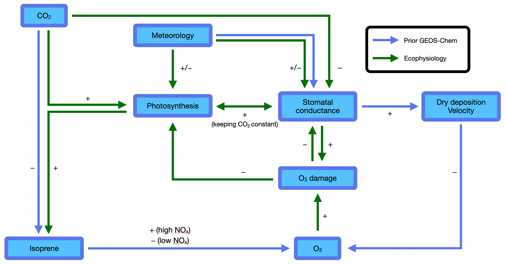
Figure 1 Atmosphere–biosphere interactions represented in the GEOS-Chem chemical transport model. Blue arrows indicate interactions included in the prior GEOS-Chem without ecophysiology. Green arrows indicate interactions added in the new ecophysiology module. The sign associated with each arrow indicates the sign of effect of one factor on another. The two arrows pointing from “Meteorology” to “Stomatal conductance” indicate that the ecophysiology module changes how meteorology affects stomatal conductance. Other species are also simulated by the GEOS-Chem and may interact with O₃ but are omitted here for simplicity.

In view of the above, a proper representation of ecophysiological processes has the potential to improve atmospheric chemistry modeling, especially in relation to biosphere–atmosphere exchange. This can be done in various ways. A CTM can be coupled with a land surface or biosphere model within an Earth system framework, whereby atmospheric processes (e.g., deposition, emissions) can be linked dynamically to biospheric processes (e.g., photosynthesis, stomatal regulation, soil biogeochemistry). For instance, Sadiq et al. (2017) and Lei et al. (2020) both examined O₃–vegetation interactions by developing a modeling framework where ozone air quality, ecophysiology, and ecosystem structure (e.g., LAI, canopy height) can co-evolve interactively. This approach is particularly useful for examining how ecosystem structure may respond to long-term atmospheric chemical changes over multidecadal timescales. However, the computation of ecosystem structure involves complex representation of plant phenology and biogeochemistry (e.g., allocation, biomass growth, senescence, mortality), which may be unnecessary for problems involving shorter timescales, e.g., seasonal responses of plant–atmosphere interactions and O₃ pollution to droughts or heat waves (e.g., Emberson et al., 2013). It also introduces extra uncertainties while not necessarily improving model performance in atmospheric chemistry. A more efficient approach is to implement process-based representation of ecophysiology into a CTM. This has been done to various extents in the past; for example, Zhang et al. (2003) implemented a semi-empirical, multiplicative scheme based on Jarvis (1976) to account for plant responses to varying radiation, temperature, VPD, and soil water stress. However, thus far the variability of r_s is still often not fully captured in CTMs. A mechanistic approach in modeling r_s should account for the ecophysiology behind, especially photosynthesis, and therefore better simulate r_s.

In this study, we developed a new ecophysiology module in the GEOS-Chem chemical transport model to dynamically simulate bulk canopy stomatal conductance g_s and plant photosynthesis A_n. Figure 1 summarizes the interactions in the prior GEOS-Chem and in the new ecophysiology module. We highlight that O₃ damage to vegetation is a key component in the model, because it allows atmospheric chemistry, in addition to meteorology, to affect plant ecophysiology and represents a more complete set of two-way interactions and feedback pathways. This development not only provides an alternative to the prior parameterization in the dry deposition module based on Wesely (1989), but also allows for biogeoscientists to study the effects of pollutant deposition on plant health, especially when simultaneously influenced by other stresses such as droughts and heat waves. By considering leaf biochemistry, boundary-layer meteorology, soil moisture stress, and O₃ deposition damage, this new module can couple physiological processes to atmospheric chemistry. We particularly aim to address the following two questions:

1. How does the ecophysiology module compare to the semi-empirical Wesely (1989) parameterization in terms of simulating concentration and dry deposition velocity of O₃, when compared to estimates based on site measurements?

2. Does the ecophysiology module simulate vegetation productivity, dry deposition, isoprene emission rate, and O₃–vegetation interactions reasonably under present-day and elevated CO₂ concentrations?

2 Model

2.1 Model description

The GEOS-Chem global chemical transport model (http://www.geos-chem.org, last access: 22 April 2023) version 12.2.0 includes detailed HO_x–NO_x–VOC–O₃–halogen–aerosol tropospheric chemistry (Bey et al., 2001). We conducted simulations at a horizontal resolution of 2^∘ latitude by 2.5^∘ longitude, driven by assimilated meteorology at an hourly time resolution from the Modern-Era Retrospective analysis for Research and Applications, Version 2 (MERRA-2) (Gelaro et al., 2017) dataset, which is an atmospheric reanalysis dataset that includes assimilation of aerosol observations. Leaf area index (LAI) values are prescribed by a gridded dataset from Yuan et al. (2011), who used gap-filling and smoothing techniques to process MODIS (Moderate Resolution Imaging Spectroradiometer) LAI. Emission data are handled by the Harmonized Emissions Component (HEMCO) v2.1 (Keller et al., 2014). HEMCO uses anthropogenic emissions of CO, NO_x, and non-methane VOCs (NMVOCs) from the Community Emissions Data System (CEDS) inventory (Hoesly et al., 2018), and the biogenic emissions of NMVOCs are computed by the Model of Emissions of Gases and Aerosols from Nature (MEGAN) version 2.1 (Guenther et al., 2012). Besides the MEGAN emission inventory, we also implemented a photosynthesis-based isoprene emission scheme following Pacifico et al. (2011) as an alternative. The scheme introduces another pathway of coupling atmospheric chemistry to ecophysiology. The detailed formulation is included in Sect. 2.1.7.

Dry deposition is modeled using the Wesely (1989) scheme but with r_s calculated from the new ecophysiology module. It is simulated for every land surface type in the Olson Land Map, which is derived from the USGS global land characteristics database (https://doi.org/10.5066/F7GB230D, Loveland et al., 2000). These land surface types are also mapped into five plant functional types (PFTs), which are used in the ecophysiology module to represent different types of vegetation. The five PFTs are broadleaf tree, needleleaf tree, C₃ grass, C₄ grass, and shrub. Each PFT has a different set of parameters, thus yielding different r_s. PFT-specific parameters (tabulated in Table S1 in the Supplement) are from Clark et al. (2011), Raoult et al. (2016), and Sitch et al. (2007). The module would skip the calculation for a PFT if it does not exist within the grid cell. The ecophysiology module also requires extra soil parameters to calculate soil moisture stress (see Sect. 2.1.5). We used gridded soil parameter data from the Hadley Centre Global Environment Model version 2 – Earth System Model (HadGEM2-ES) to calculate the soil moisture stress function (details in Sect. 2.1.5). Besides r_s, vegetation-related outputs such as gross photosynthetic uptake of carbon, canopy dark respiration, and canopy O₃ uptake are also available. The formulations in the ecophysiology module were adopted from the Joint UK Land Environmental Simulator (JULES) (Best et al., 2011; Clark et al., 2011). Important ones are included below, and others are detailed in the Supplement.

2.1.1 Leaf biochemistry

Formulations of photosynthesis rates for C₃ and C₄ plants were derived from leaf biochemistry and formulated as in Collatz et al. (1991) and Collatz et al. (1992), respectively. They are calculated from the three potentially limiting rates, each as a function of c_i and some other meteorological variables (see the Supplement).

The leaf-level net photosynthesis (A_n, $\mathrm{\mu }\mathrm{mol}{\mathrm{CO}}_{\mathrm{2}}{\mathrm{m}}^{-\mathrm{2}}{\mathrm{s}}^{-\mathrm{1}}$) is calculated as a smoothed minimum (see the Supplement) of the 3 potentially limiting rates (W_c, W_l, W_e, $\mathrm{\mu }\mathrm{mol}{\mathrm{CO}}_{\mathrm{2}}{\mathrm{m}}^{-\mathrm{2}}{\mathrm{s}}^{-\mathrm{1}}$) minus dark respiration (R_d, $\mathrm{\mu }\mathrm{mol}{\mathrm{CO}}_{\mathrm{2}}{\mathrm{m}}^{-\mathrm{2}}{\mathrm{s}}^{-\mathrm{1}}$):

$$\begin{array}{}\text{(1)}& A_{\mathrm{n}}=min(W_{\mathrm{c}},W_{\mathrm{l}},W_{\mathrm{e}})-R_{\mathrm{d}},\end{array}$$

where R_d is linearly proportional to V_cmax by the dark respiration coefficient f_dr:

$$\begin{array}{}\text{(2)}& R_{\mathrm{d}}=f_{\text{dr}}{V}_{\text{cmax}}.\end{array}$$

2.1.2 Photosynthesis as a diffusive flux

The leaf-level net photosynthesis A_n can also be represented as a diffusive flux of CO₂ modulated by the leaf-level stomatal conductance g_s0 (m s⁻¹). Therefore, we can find g_s0 using

$$\begin{array}{}\text{(3)}& g_{\text{s0}}={\displaystyle \frac{\mathrm{1.6}\times {\mathrm{10}}^{-\mathrm{6}}{A}_{\mathrm{n}}}{c_{\mathrm{c}}-c_i}}{R}_{\ast }T,\end{array}$$

where c_c is the canopy CO₂ partial pressure (Pa), the number 1.6 accounts for different diffusivities of CO₂ and H₂O through leaf stomata, R_∗ = 8.31 $\mathrm{J}{\mathrm{K}}^{-\mathrm{1}}{\mathrm{mol}}^{-\mathrm{1}}$ is the universal molar gas constant, and T is the canopy air temperature (K). We assume c_c and T to be equal to the ambient CO₂ concentration and the 2 m temperature, respectively.

2.1.3 Canopy scaling

A simple big-leaf approach is applied to scale up leaf-level variables to the canopy-level variables. It is assumed that incident light is attenuated by the canopy according to Beer's law:

$$\begin{array}{}\text{(4)}& I\left(L\right)=I_{\mathrm{0}}{e}^{-kL},\end{array}$$

where I(L) and I₀ are the irradiance at the height of the canopy with cumulative leaf area index L and at the top of the canopy, respectively, and k is the PAR extinction coefficient of the canopy. Detailed formulations can be found in the Supplement.

2.1.4 Stomatal closure parameterization

A third equation by Jacobs (1994) relating c_i and g_s via canopy humidity deficit D (${\mathrm{kg}}_{\mathrm{w}}{\mathrm{kg}}_{\mathrm{a}}^{-\mathrm{1}}$) is included to obtain a closed set of equations for A_n, g_s0, and c_i. This formulation was discussed in detail by Cox et al. (1998).

$$\begin{array}{}\text{(5)}& {\displaystyle \frac{c_i-\mathrm{\Gamma }}{c_{\mathrm{c}}-\mathrm{\Gamma }}}=f_{\mathrm{0}}\left(\mathrm{1}-{\displaystyle \frac{D}{D_{\ast }}}\right),\end{array}$$

where f₀ and D_∗ are PFT-specific parameters. D is evaluated as the difference between the saturation specific humidity (${\mathrm{kg}}_{\mathrm{w}}{\mathrm{kg}}_{\mathrm{a}}^{-\mathrm{1}}$) evaluated at leaf temperature T_l and the 2 m specific humidity. If we assume a thin leaf boundary layer, T_l would be equal to the 2 m air temperature.

Table 1 Configuration of the first set of simulations that evaluate the modeled concentration and dry deposition velocity of ozone (O₃).

2.1.5 Soil moisture stress

Under dry soil conditions, A_n, R_d, and g_s0 are reduced due to limited availability of water. An extra factor β_t, which ranges from 0 to 1, is multiplied to all three quantities. It is modeled as

$$\begin{array}{}\text{(6)}& {\mathit{\beta }}_{\mathrm{t}}=\left\{\begin{array}{ll}\mathrm{1}& \text{for }\mathit{\theta }>{\mathit{\theta }}_{\mathrm{c}},\\ \frac{\mathit{\theta }-{\mathit{\theta }}_{\mathrm{w}}}{{\mathit{\theta }}_{\mathrm{c}}-{\mathit{\theta }}_{\mathrm{w}}}& \text{for }{\mathit{\theta }}_{\mathrm{w}}<\mathit{\theta }\le {\mathit{\theta }}_{\mathrm{c}},\\ \mathrm{0}& \text{for }\mathit{\theta }\le {\mathit{\theta }}_{\mathrm{w}},\end{array}\right.\end{array}$$

where $\mathit{\theta }=S\times {\mathit{\theta }}_{\mathrm{s}}$ is the root zone soil moisture; S is the root zone soil wetness (in terms of fraction of soil pore space); and θ_s, θ_c, and θ_w are the saturation, critical, and wilting soil moisture variables, respectively. We use the soil ancillary maps that contain θ_s, θ_c, and θ_w at 0.5^∘ × 0.5^∘ resolution from HadGEM2-ES.

2.1.6 O₃ damage

The O₃ damage scheme in JULES is based on Sitch et al. (2007). When the ambient O₃ concentration is high enough, A_n, R_d, and g_s0 are further reduced due to O₃ damage to plant cells. An O₃ damage factor ${\mathit{\beta }}_{{\mathrm{O}}_{\mathrm{3}}}$, which ranges from 0 to 1, is multiplied to the three quantities. The damage factor is given by

$$\begin{array}{}\text{(7)}& {\mathit{\beta }}_{{\mathrm{O}}_{\mathrm{3}}}=\mathrm{1}-a\times max[F_{{\mathrm{O}}_{\mathrm{3}}}-F_{{\mathrm{O}}_{\mathrm{3}}\mathrm{crit}},\mathrm{0}],\end{array}$$

where $F_{{\mathrm{O}}_{\mathrm{3}}}$ is the O₃ deposition flux through stomata ($\mathrm{nmol}{\mathrm{m}}^{-\mathrm{2}}{\mathrm{s}}^{-\mathrm{1}}$), $F_{{\mathrm{O}}_{\mathrm{3}}\mathrm{crit}}$ is the threshold for stomatal O₃ uptake ($\mathrm{nmol}{\mathrm{m}}^{-\mathrm{2}}{\mathrm{s}}^{-\mathrm{1}}$), and a is the gradient of the O₃ dose response function (nmol⁻¹ m² s); a and $F_{{\mathrm{O}}_{\mathrm{3}}\mathrm{crit}}$ are PFT-specific parameters. There are two sets of values of a corresponding to “high” and “low” sensitivities. The stomatal O₃ deposition flux is modeled using a flux gradient approach:

$$\begin{array}{}\text{(8)}& F_{{\mathrm{O}}_{\mathrm{3}}}={\displaystyle \frac{\left[{\mathrm{O}}_{\mathrm{3}}\right]}{r_{\mathrm{a}}+r_{\mathrm{b}}+{\mathit{\kappa }}_{{\mathrm{O}}_{\mathrm{3}}}{r}_{\mathrm{s}}}}\end{array}$$

where [O₃] is the molar concentration of O₃ at the lowest model level, r_a is the aerodynamic resistance (s m⁻¹), r_b is the quasi-laminar sublayer resistance, r_s = $\mathrm{1}/g_{\mathrm{s}}$ is the stomatal resistance, and ${\mathit{\kappa }}_{{\mathrm{O}}_{\mathrm{3}}}$ = 1.61 accounts for the relative difference in diffusivities of O₃ and H₂O through leaf stomata. Since r_s in Eq. (8) depends on ${\mathit{\beta }}_{{\mathrm{O}}_{\mathrm{3}}}$, Eqs. (7) and (8) can be combined into a quadratic equation and solved analytically to give ${\mathit{\beta }}_{{\mathrm{O}}_{\mathrm{3}}}$.

2.1.7 Photosynthesis-dependent isoprene emission

In the default GEOS-Chem, canopy isoprene emission is computed by MEGAN v2.1, which calculates biogenic VOC emissions of various species as functions of canopy-scale PFT-specific emission factors modulated by environmental activity factors to account for changing temperature, light, leaf age, and LAI, weighted by the PFT fraction in each grid cell to give the grid-cell-level emission fluxes. The activity factors are essentially semi-empirical functions constrained by experimental data and are not explicitly linked to mechanistic ecophysiological processes. Here in the ecophysiology module, canopy isoprene emission (E_isoprene, $\mathrm{kg}\mathrm{C}{\mathrm{m}}^{-\mathrm{2}}{\mathrm{s}}^{-\mathrm{1}}$) is linked explicitly to photosynthesis, based on Pacifico et al. (2011):

$$\begin{array}{}\text{(9)}& E_{\text{isoprene}}=\mathrm{IEF}{\mathit{\rho }}_{\text{leaf}}{\displaystyle \frac{A_{\mathrm{c}}+R_{\text{dc}}}{(A_{\mathrm{n}}{)}_{\text{st}}+(R_{\mathrm{d}}{)}_{\text{st}}}}{f}_T{f}_{{\mathrm{CO}}_{\mathrm{2}}},\end{array}$$

where IEF is the PFT-specific isoprene emission factor ($\mathrm{\mu }\mathrm{g}\mathrm{C}\mathrm{g}{\mathrm{dw}}^{-\mathrm{1}}{\mathrm{h}}^{-\mathrm{1}}$, where “dw” means dry weight), i.e., base emission rate of isoprene at the leaf level under standard conditions (i.e., temperature of 30 ^∘C, photosynthetically active radiation of 1000 $\mathrm{\mu }\mathrm{mol}{\mathrm{CO}}_{\mathrm{2}}{\mathrm{m}}^{-\mathrm{2}}{\mathrm{s}}^{-\mathrm{1}}$, CO₂ concentration of 370 ppm, and without any O₃ damage or soil moisture stress), ρ_leaf is the dry leaf area density ($\mathrm{g}{\mathrm{dw}}^{-\mathrm{1}}{\mathrm{m}}^{-\mathrm{2}}$), f_T and $f_{{\mathrm{CO}}_{\mathrm{2}}}$ are temperature- and CO₂-dependent empirical factors to account for variation with changing temperature and CO₂ level (see the Supplement for detailed formulations). Variables with subscript “st” are calculated under standard conditions. We note that, as opposed to Pacifico et al. (2011), our model does not capture a reduction in c_i following soil moisture limitation, because we use prescribed 2 m specific humidity data in the meteorological input to calculate c_i. The effect of soil moisture stress on isoprene emission is only captured in the calculation of A_c and R_dc. This may lead to a lower isoprene emission rate compared to the original scheme, but direct comparison is not possible due to different input meteorology used in our study.

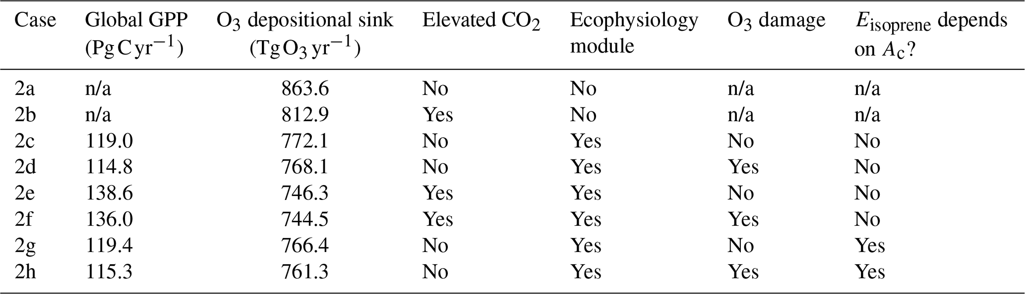
Table 2 Configuration of the second set of simulations that investigate gross primary production (GPP) and ozone (O₃) concentration under an elevated CO₂ scenario.

2.2 Experimental design

To evaluate the modeled concentration and dry deposition velocity of O₃, we conduct four 1-year simulations from 1 January 2012 to 1 January 2013 using GEOS-Chem v12.2.0 driven by offline MERRA-2 meteorology. A half-year spin-up is conducted before the simulation period. Table 1 summarizes the configurations of each simulation. A control case (case 0) uses the GEOS-Chem v12.2.0 with prior input configuration, while the other three cases (1a–c) use the modified GEOS-Chem with ecophysiology module turned on. Each of the three cases use different O₃ damage sensitivities. We then compare the modeled concentration and dry deposition velocity of O₃ against site observations. Year 2012 is chosen as the simulation year to maximize the number of observations that our results can be evaluated against.

We also conduct a second set of simulations from 1 January 2000 to 1 January 2001 to demonstrate the capability of the new module to simulate changes in plant productivity in response to changing CO₂ and subsequent changes in atmospheric chemistry. A half-year spin-up is conducted before the simulation period. The simulations are set up with only CO₂ being changed, while meteorological and other inputs remain unchanged. Table 2 summarizes the configuration of each simulation. Case 2a is the control experiment where prior configuration from the GEOS-Chem is used. Case 2b simulates the effect of elevated CO₂ on stomatal conductance by using the CO₂–g_s scaling factor described in Franks et al. (2013) (details are included in the Supplement) and setting the ambient CO₂ concentration to 580 ppm, which is approximately the projected CO₂ concentration around the 2050s in a business-as-usual scenario (e.g., Representative Concentration Pathway 8.5). This simple scaling approach has been suggested to investigate how rising CO₂ may affect ozone dry deposition in the future. This now allows us to compare between the mechanistic ecophysiology module, which simulates plant responses to rising CO₂ more mechanistically, and the semi-empirical CO₂–g_s scaling factor in the context of O₃ concentration and depositional sink. Cases 2c–f are conducted to compare the O₃ depositional sink and concentration to cases 2a–b, as well as to investigate how GPP and O₃ depositional sink change under an elevated CO₂ scenario. Cases 2g–h are duplicates of 2c–d, respectively, except that the isoprene emission rates are calculated using a photosynthesis-based scheme from Pacifico et al. (2011) instead of from the prior MEGAN emission inventory. They reveal whether the photosynthesis-based scheme yields a reasonable estimate of global isoprene emission under our model.

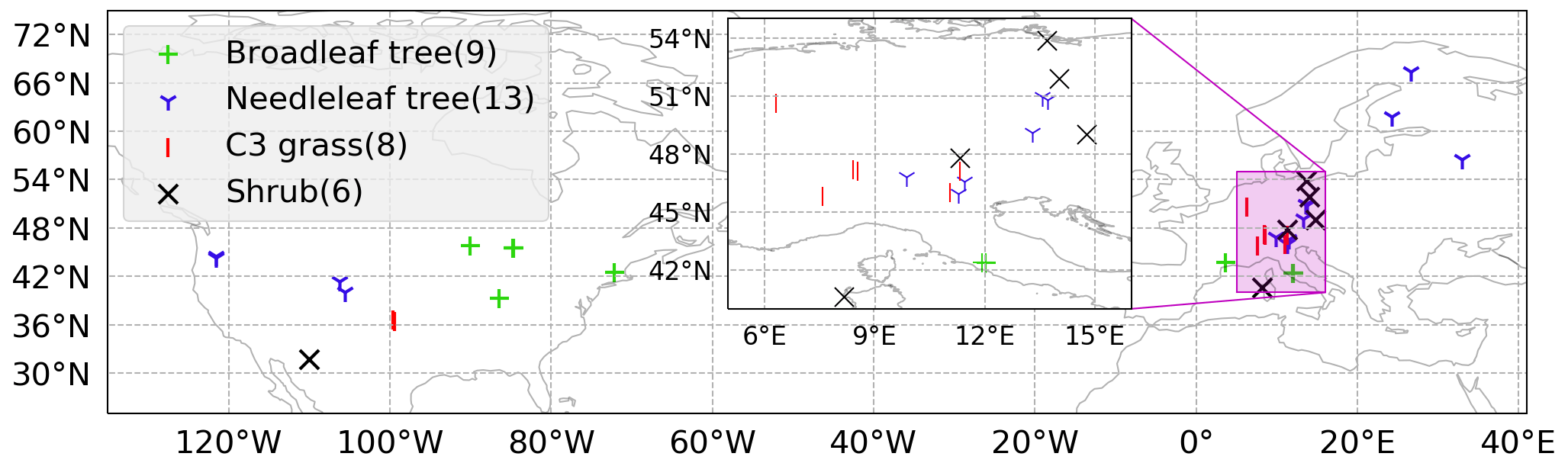
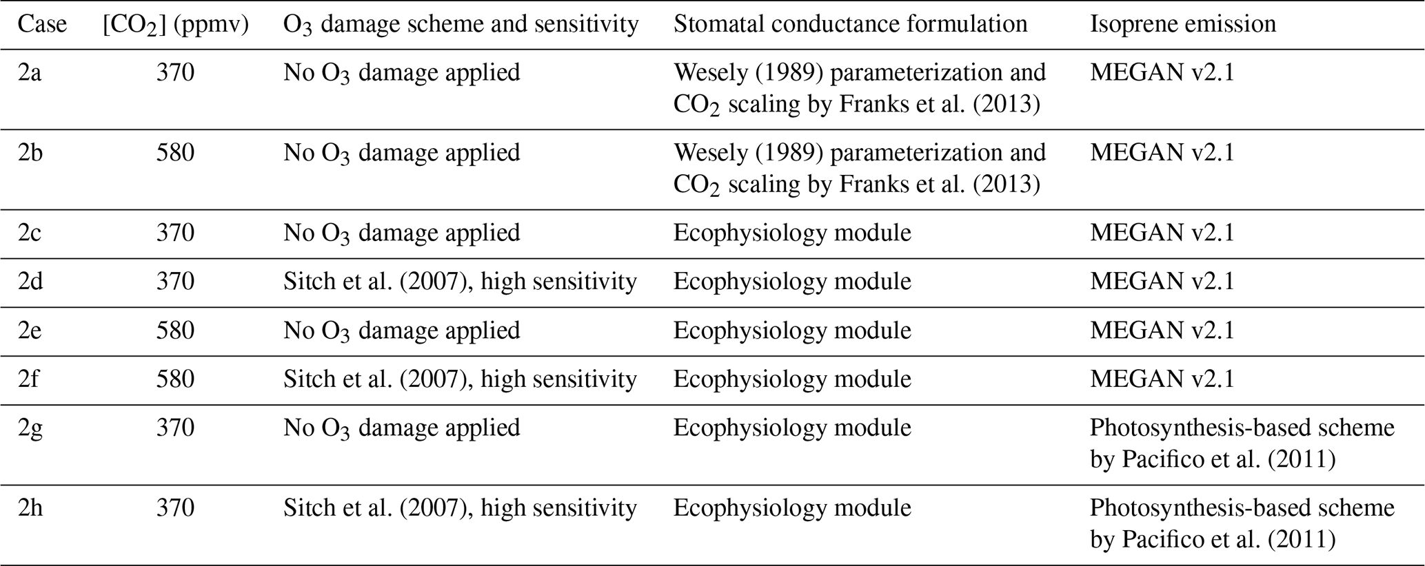
Figure 2 Locations of 36 SynFlux sites used in the evaluation of the ecophysiology module. Different symbols indicate different plant functional types (PFTs) as broadleaf tree (green “+”, includes evergreen broadleaf tree, EBF, and deciduous broadleaf tree, DBF), needleleaf tree (blue “Y”, includes evergreen needleleaf tree (ENF) only), C₃ grass (red “|”, includes grassland (GRA) only), and shrub (black “X”, includes wetland, WET, open shrubland, OSH, and closed shrubland, CSH). The number of sites for each PFT is in parentheses in the legend. Two C₄ grass (including savanna, SAV, and woody savanna, WSA) sites are ignored in our evaluation due to a lack of observational data in our simulation period. Mixed forest (MF) and cropland (CRO) sites are not classified into any of the PFTs, because they are usually composed of multiple PFTs.

2.3 Evaluation data: SynFlux

We evaluate the modeled dry deposition velocity and concentration of O₃ against an observationally derived dataset known as Synthetic O₃ Flux (SynFlux) (Ducker et al., 2018). It derives site-level v_d by combining eddy covariance measurements of micrometeorological flux from FLUXNET sites in the United States and Europe with a gridded dataset of O₃ concentration. The aerodynamic and quasi-laminar sublayer resistances r_a and r_b from each of the sites are derived from the meteorological quantities measured at the sites. The surface conductance (reciprocal of resistance) is a summation of two components: stomatal conductance g_s and non-stomatal conductance g_ns; g_s is derived from the measured water vapor flux and meteorological data, and g_ns is estimated using Zhang et al. (2003). Figure 2 shows the locations of 36 SynFlux sites used in our evaluation of the ecophysiology module. All sites with available data within the simulation interval are selected. The total number of sites for each PFT is listed in the legend of Fig. 2. There are only two sites that represent C₄ grass, and they are ignored because observational data are only available in August. The SynFlux dataset was evaluated at three sites with direct O₃ flux measurements. The synthetic stomatal O₃ flux strongly correlates with measurements (R² = 0.83–0.93), and the mean bias is modest (21 % or less). In addition, 95 % of the SynFlux values differ from measurements by less than a factor of 2. The errors in SynFlux have been shown to be modest compared with differences between observations and regional and global CTMs that are frequently a factor of 2 or more, illustrating its utility for evaluating models (Ducker et al., 2018).

3 Results

3.1 Comparison between ecophysiology module and prior Wesely (1989) parameterization

We compare the modeled PFT-specific dry deposition velocity v_d and stomatal conductance g_s of O₃ in summer (JJA) to SynFlux. The modeled v_d and g_s were obtained by averaging hourly outputs from June to August 2012. They were then paired up with the SynFlux dataset by matching the month, location, and PFT. In Figs. 3 and 4, the model results on model grid cells closest to the SynFlux sites are plotted against the corresponding observation-derived estimates from SynFlux for each PFT. C₄ grass is ignored due to a lack of observational data. The soil moisture stress factor β_t on the corresponding model grid is represented by the color of the circle.

Figure 3 Plots of modeled monthly mean dry deposition velocity of O₃ (cm s⁻¹) in northern summer (JJA) against SynFlux estimates, categorized by site PFT for each simulation case. Columns from right to left represent simulation cases 0 and 1a, respectively. Each row corresponds to a PFT. C₄ grass is ignored due to a lack of observational data. The soil moisture stress factor β_t on the corresponding model grid cell is represented by the color of the circle. Mean bias (MB) and root-mean-squared error (RMSE) are shown for each plot. Full results including cases 1b and 1c can be found in the Supplement.

Figure 4 Same as Fig. 3 but for monthly mean stomatal conductance g_s (cm s⁻¹) under the β_t≠0 condition. For results including β_t = 0 condition, please refer to Fig. S2.

Figure 3 shows that the ecophysiology module reduces the overestimation in v_d by the prior dry deposition module, especially for broadleaf trees, for which the root-mean-squared error (RMSE) decreases from 0.48 to 0.11 cm s⁻¹. C₃ grass shows a similar change where the RMSE decreases from 0.36 to 0.21 cm s⁻¹ in case 1c (see Fig. S1 in the Supplement), where high O₃ damage sensitivity is applied. C₃ grass is the most sensitive to O₃ damage among the four PFTs as the modeled v_d varies the most under different O₃ damage sensitivities. For needleleaf tree, the overestimation without the ecophysiology module becomes underestimated, regardless of the sensitivity of O₃ damage. O₃ damage barely affects v_d.

Figure 4 shows that the ecophysiology module significantly improves the simulation of g_s for broadleaf trees, needleleaf trees, and shrubs, excluding those simulated with a soil moisture stress factor of β_t = 0. This exclusion is due to the assumption that the soil moisture stress parameterization is not well calibrated in the ecophysiology module. The results without the exclusion are available in Fig. S2. The RMSEs for both broadleaf trees and needleleaf trees decrease from 0.90 and 0.75 to 0.15 and 0.21 cm s⁻¹, respectively. For shrubs, the RMSE also decreases from 0.50 to 0.03–0.04 cm s⁻¹ (depending on sensitivity of O₃ damage applied, see Fig. S2). For C₃ grass, the mechanistic formulation slightly decreases g_s, which is consistent with the results in Fig. 3. Combining the validation of v_d and g_s, we find that the lower v_d as simulated by the ecophysiology module is attributable to photosynthesis-based stomatal conductance being generally smaller than that estimated by the semiempirical formulation, which was also discussed by Wong et al. (2019).

In Figs. 3–5, the colors of circles represent the soil moisture stress factor β_t described in Sect. 2.1.5. In the semi-empirical parameterization, v_d and g_s do not depend on β_t. However, v_d and g_s simulated using the ecophysiology module are significantly affected by β_t as v_d and g_s with low β_t are almost always lower than those with high β_t, regardless of site locations. Also, for broadleaf trees and needleleaf trees, low β_t values appear to result in a nearly constant value of v_d = 0.2 cm s⁻¹, reflecting mostly non-stomatal deposition, while high β_t gives a much closer estimate of g_s and v_d to observations. Since g_s is multiplied by β_t as described in Sect. 2.1.5, low β_t values should indeed give lower g_s and thus lower v_d. At different site locations, other components of v_d can also vary, but the strong correlation between β_t and v_d remains. Whether v_d is sensitive to vapor pressure deficit (VPD) in a similar fashion arguably warrants further investigation. Overall, our results indicate that β_t is an important parameter in this formulation and strongly affects the model performance on simulating dry deposition velocity. However, there is a large inter-model variation in β_t due to variability in soil moisture, different formulations of β_t, and vertical resolution of soil levels (Trugman et al., 2018). Since GEOS-Chem does not simulate soil explicitly, we only use a simple and empirical parameterization of β_t with input of a single-layer soil moisture from the MERRA-2 dataset. Such deficiency in the representation of β_t may render the model less reliable in simulating the potential impact of drought events on atmospheric chemistry and plant productivity. Therefore, simulation of drought events, which is one of the potential uses of the ecophysiology module, should be interpreted cautiously unless parameters in the β_t function are more thoroughly calibrated on a regional or local basis. Despite the uncertainty of β_t, we emphasize that including the stomatal responses to VPD and soil moisture is valuable, because the Wesely (1989) parameterization cannot represent such stomatal responses. We also compare the model results of monthly mean O₃ concentration in summer with SynFlux estimates, derived from a gridded dataset of O₃ concentration. Figure 5 shows the comparison of monthly mean O₃ concentration on model grid cells closest to the SynFlux sites against the corresponding estimates from SynFlux categorized by site PFT. According to the rightmost column, O₃ concentration is originally overestimated by the GEOS-Chem model. The ecophysiology module increases the model bias by 4 to 5 ppbv for broadleaf trees, needleleaf trees, and C₃ grasses, and by 2 ppbv for shrubs. Activation of the O₃ damage scheme and the change of sensitivity to O₃ damage only produce modest differences (see Fig. S3) in terms of monthly mean O₃ concentration, representing relatively weak O₃–vegetation feedback effects.

Figure 5 Same as Fig. 3 but for modeled monthly mean O₃ concentration (ppbv).

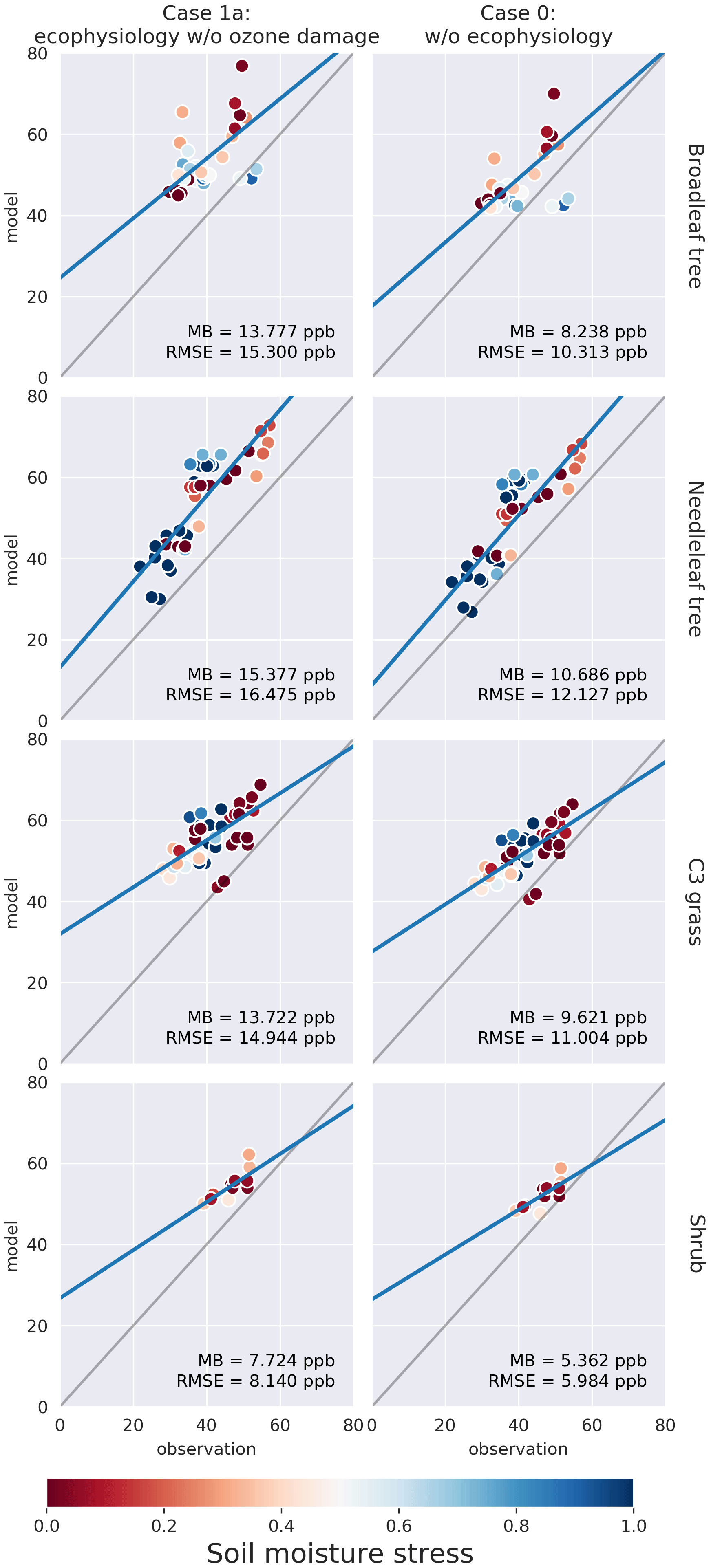
There can be multiple possible reasons leading to the biases in O₃ concentration. First, the simulated O₃ concentration on nearby model grid cells is only a bulk average over the entire area of the grid cell, while the measurement reflects the local O₃ concentration. Subgrid variability created by local meteorology or surface topography is not accounted for during the comparison. Unlike dry deposition velocity, it is not possible to separate O₃ concentration into a PFT-specific quantity for a fair comparison. Secondly, accurate simulation of O₃ relies on many non-stomatal depositional and non-depositional processes as well, e.g., chemistry, photochemistry, and emissions of precursor gases. Since we show that simulation of dry deposition velocity of O₃ is improved by the ecophysiology module, modifications in non-stomatal depositional and non-depositional processes would be required more urgently to improve the performance in O₃ simulations. The problems of general overestimation of O₃ by various models at northern midlatitudes have been discussed by Travis et al. (2016).

Table 3 Annual global GPP and total O₃ depositional sink in each simulation.

n/a: not applicable

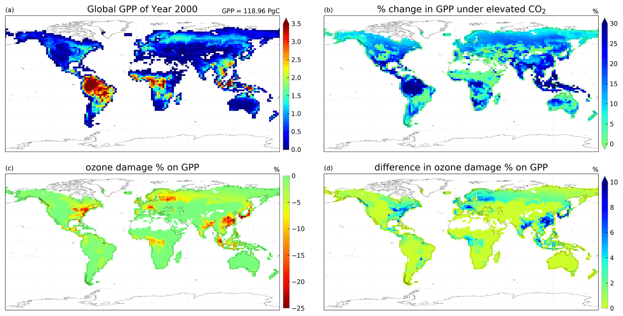
Figure 6 Maps of (a) global GPP distribution ($\mathrm{kg}\mathrm{C}{\mathrm{m}}^{-\mathrm{2}}{\mathrm{yr}}^{-\mathrm{1}}$) in case 2c, (b) percentage change in GPP driven by CO₂ concentration increase, (c) percentage change in GPP driven by high-sensitivity O₃ damage, and (d) difference in O₃-driven percentage change in GPP between experiments with year 2000 and elevated CO₂ concentrations, where the positive values indicate a reduction in ozone damage.

3.2 GPP and O₃ depositional sink simulated by the ecophysiology module under different CO₂ levels

In the second set of simulations, we demonstrate that with the new dynamic linkage to ecophysiology, the model is capable of capturing CO₂–O₃–vegetation interactions under elevated CO₂ concentration. Table 3 tabulates the global GPP and the O₃ depositional sink for each of the cases, and Fig. 6 shows their spatial distributions. Under the year 2000-level CO₂ scenario, the simulated gross primary production (GPP) is 119 Pg C yr⁻¹, and the total O₃ depositional sink is 772 Tg O₃ yr⁻¹ in the absence of O₃ damage. The global O₃ deposition flux is close to the mean value from 12 CTMs (747 Tg O₃ yr⁻¹) used in the Third Assessment Report of the Intergovernmental Panel on Climate Change (IPCC TAR) (Prather and Ehhalt, 2001), but it is generally lower than the values from later multi-model studies, e.g., 1003 ± 200 Tg O₃ yr⁻¹ from Stevenson et al. (2006) and 902 ± 255 Tg O₃ yr⁻¹ from Wild (2007). A possible reason is that most CTMs use a semi-empirical formulation of the stomatal conductance, which is generally larger than ecophysiology-based stomatal conductance (Wong et al., 2019), and thus higher dry deposition fluxes in other CTMs are expected. Globally, the O₃ damage on GPP is 4.2 Pg C yr⁻¹ (3.5 %), but the O₃ damage percentage can reach more than 20 % regionally, e.g., in China, as shown in Fig. 6c.

Figure 7 Monthly gross primary production (GPP) ($\mathrm{g}\mathrm{C}{\mathrm{m}}^{-\mathrm{2}}{\mathrm{month}}^{-\mathrm{1}}$) for simulation cases 2c–f for (a) all PFTs, (b) broadleaf trees, (c) needleleaf trees, (d) C₃ grasses, (e) C₄ grasses, and (f) shrubs. Blue and green lines denote simulation cases under year 2000 and elevated CO₂ level, respectively. Darker and brighter lines denote cases with and without O₃ damage, respectively.

Under elevated CO₂ scenario (case 2e minus 2c), GPP is projected to increase by 19.7 Pg C yr⁻¹ (16.8 %) globally and up to 30 % regionally near the tropics (Fig. 6b). We note also that such changes in GPP are entirely due to higher photosynthetic rate, since LAI is prescribed. The global O₃ depositional flux decreases by 25.8 Tg O₃ yr⁻¹ (3.3 %). This change is about half of that given by the CO₂–g_s scaling factor experiments (cases 2b minus 2a), implying that, compared to the simple CO₂–g_s scaling factor, the mechanistic ecophysiology module predicts less reduction in stomatal conductance at a higher CO₂ level. It should be noted that the semi-empirical CO₂–g_s scaling factor is an approximation based only on the RuBP-limited photosynthesis rate (Franks et al., 2013) and thus does not necessarily represent the full range of limiting or compensating conditions for photosynthesis. The magnitude of O₃ percentage damage is reduced by around 10 percentage points (i.e., the percentage damage goes from about −20 % to −10 %) in regions with originally high O₃ damage such as southern China, Europe, and the eastern USA (Fig. 6d). The monthly distribution of GPP also generally agrees with results from other models. Figure 7a shows the monthly distribution of global GPP, and Fig. 7b–f show the area-weighted average GPP for each of the PFTs. Our results demonstrate a seasonal cycle of GPP that peaks at around 130 $\mathrm{g}\mathrm{C}{\mathrm{m}}^{-\mathrm{2}}{\mathrm{month}}^{-\mathrm{1}}$ in July and falls steadily to around 60 $\mathrm{g}\mathrm{C}{\mathrm{m}}^{-\mathrm{2}}{\mathrm{month}}^{-\mathrm{1}}$ in February. This resembles observation-derived datasets like FLUXNET-MTE, as shown in Fig. 3a of Slevin et al. (2017). When the seasonal cycle of GPP for each PFT is considered separately, different trends and features are present. For broadleaf trees, the average GPP stays around 150 to 200 $\mathrm{g}\mathrm{C}{\mathrm{m}}^{-\mathrm{2}}{\mathrm{month}}^{-\mathrm{1}}$ throughout a year and is slightly higher in northern summer. C₄ grasses also have a steady average GPP of around 100 to 150 $\mathrm{g}\mathrm{C}{\mathrm{m}}^{-\mathrm{2}}{\mathrm{month}}^{-\mathrm{1}}$ but have an opposite cycle to all other PFTs. For needleleaf trees, C₃ grasses, and shrubs, GPP is very low in northern winter, but for needleleaf trees, it rises to more than 200 $\mathrm{g}\mathrm{C}{\mathrm{m}}^{-\mathrm{2}}{\mathrm{d}}^{-\mathrm{1}}$ in July, which is the highest among all PFTs. Under the elevated CO₂ scenario, GPP is projected to rise by 10 to 30 $\mathrm{g}\mathrm{C}{\mathrm{m}}^{-\mathrm{2}}{\mathrm{month}}^{-\mathrm{1}}$, being higher in northern summer, and vice versa. Most of the increase in GPP can be attributed to broadleaf trees and needleleaf trees, which have larger total leaf surface area than grasses and shrubs, thus amplifying the enhanced photosynthesis under higher ambient CO₂ concentration, as suggested by Eq. (S8) in the Supplement. On the other hand, C₄ grasses show no change in average GPP throughout a year.

O₃ concentration only changes moderately under elevated CO₂ concentration overall but with larger changes happening in some regions. Figure 8 shows the change in annual mean O₃ concentration under the increase in CO₂ concentration for cases 2b and 2e. In addition to larger increases of up to 3 ppbv found in the Amazon forest and Borneo regions, smaller increases of up to 1 ppbv are also found in central Africa, Southeast Asia, and at middle-to-high latitudes. This agrees with the simulation result using the CO₂–g_s scaling factor (case 2b). The latter shows even stronger increases in O₃ concentration over the Amazon forest, central Africa, and Southeast Asia.

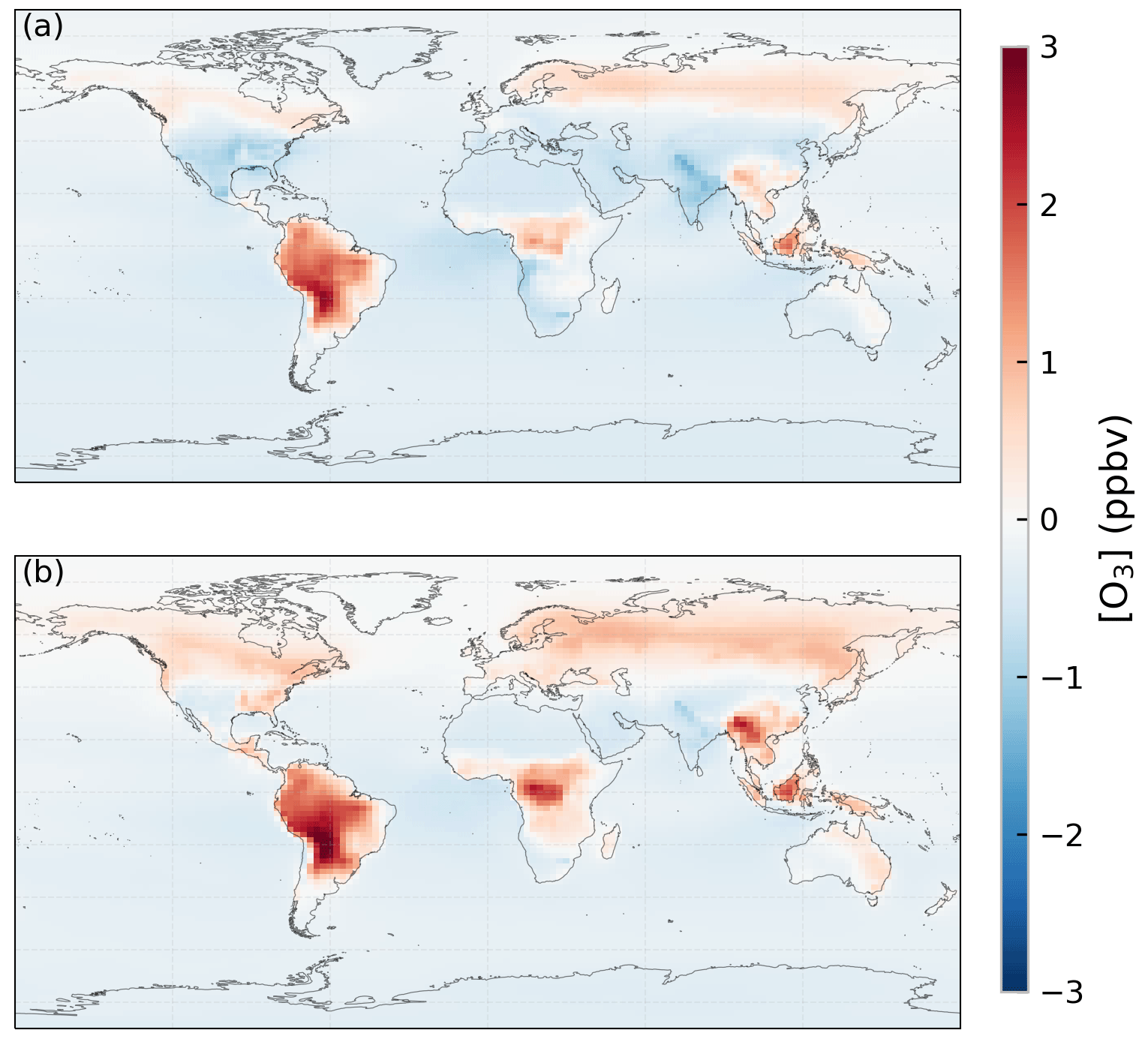
Figure 8 Changes in ozone (O₃) concentration (ppbv) due to the increase in CO₂ concentration simulated using (a) the ecophysiology module and (b) the CO₂–g_s scaling factor.

Figure 9 Annual mean isoprene emission rates ($\mathrm{g}\mathrm{C}{\mathrm{m}}^{-\mathrm{2}}{\mathrm{yr}}^{-\mathrm{1}}$) for year 2000 simulated using (a) the MEGAN emission model (case 2c) and (b) the Pacifico et al. (2011) scheme coupled with the ecophysiology module without O₃ damage (case 2g), as well as the differences in mean isoprene emission rates due to (c) switching emission schemes (case 2g minus 2c) and (d) O₃ damage on photosynthesis, which is proportional to isoprene emission rates (case 2h minus 2g). The number on the top right corner denotes the area-weighted total of emitted isoprene. White color in the figures denotes zero value.

3.3 Comparison of isoprene emission rates between photosynthesis-dependent formulation and MEGAN v2.1 emission model

Implementing a photosynthesis-dependent isoprene emission scheme into the GEOS-Chem introduces another interaction between ecophysiology and atmospheric chemistry. Here, we demonstrate that the simulated isoprene emission rates are close to what the MEGAN emission algorithm simulates. The annual isoprene emission rates in the year 2000 using the MEGAN emission inventory (case 2c) and the photosynthesis-dependent scheme from Pacifico et al. (2011) (case 2g) are shown in Fig. 9a and b, and the annual totals are 349.1 and 317.9 Tg C, respectively. The annual isoprene emission totals are at the lower end of other published estimates of 300–530 Tg C (as summarized in Table 3 in Weng et al., 2020) but are consistent with Weng et al. (2020), who estimated 330–345 Tg C yr⁻¹ using the MEGAN v2.1 at a finer spatial resolution than this study. The monthly averages of land surface temperature in the year 2000 are lower than the 2000–2009 monthly averages (see Fig. S4), which can lower the emission total. The simulated isoprene emission rate is similar to the MEGAN emission model in general, as the tropics, especially the Amazon forest, contributes the most to the annual isoprene emission total. There are, however, some modest differences in the magnitude and location of the largest emission flux in each of the continents, e.g., from −15 to +10 $\mathrm{g}\mathrm{C}{\mathrm{m}}^{-\mathrm{2}}{\mathrm{yr}}^{-\mathrm{1}}$ in different parts of South America and about −5 $\mathrm{g}\mathrm{C}{\mathrm{m}}^{-\mathrm{2}}{\mathrm{yr}}^{-\mathrm{1}}$ in the southern USA and Australia. Since the isoprene emission rate is proportional to the photosynthesis rate as in Eq. (9), these differences can be due to the simple classification of PFTs, which can constrain the maximum photosynthesis capacity and thus the photosynthesis rate. We also note that the MEGAN emission model is also subject to uncertainties in its algorithm. Besides, temperature variability in the subgrid scale is often a major source of uncertainty, since a temperature difference of +1 ^∘C is equivalent to a +10 % increase in isoprene emission rate, as inferred from Eq. (S17). Figure 9d shows that global isoprene emission decreases by 12.1 Tg C yr⁻¹ (3.8 %) (case 2h minus 2g) due to O₃ damage to vegetation. This reduction is mainly due to the 3.5 % decrease in GPP via the dry deposition pathway, as described in Sect. 3.2.

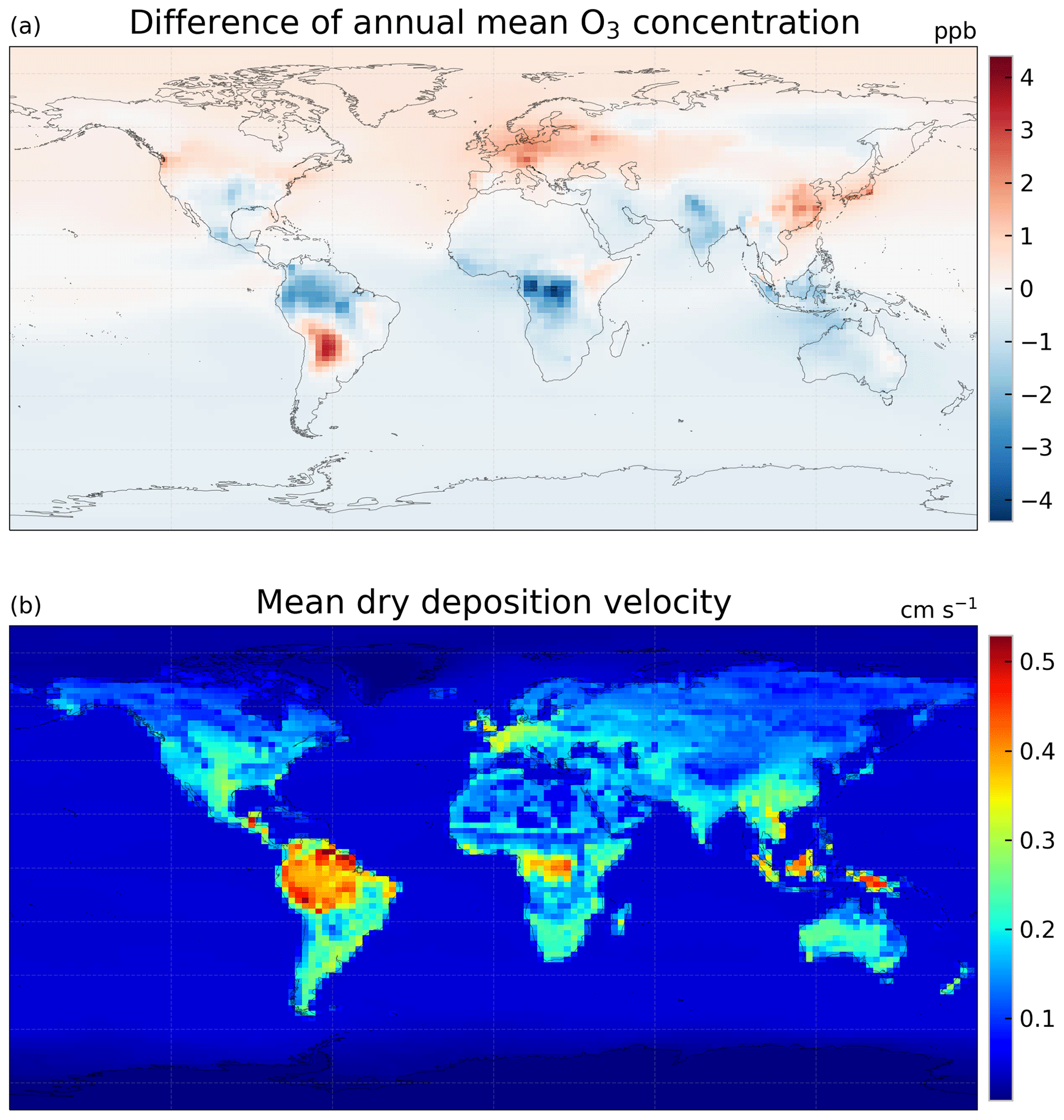
Figure 10 (a) Difference in annual mean O₃ concentration (ppbv) between using the MEGAN emission model and the Pacifico et al. (2011) photosynthesis-based isoprene emission scheme (case 2g minus 2c) and (b) annual mean dry deposition velocity of O₃ (cm s⁻¹) simulated with the ecophysiology module (case 2g, and it should be very similar to case 2c).

In terms of GPP and O₃ depositional sink, switching isoprene emission scheme from the MEGAN emission model to a photosynthesis-based scheme by Pacifico et al. (2011), i.e., comparing case 2c to case 2g, does not change the GPP when O₃ damage is absent, as shown in Table 3. This is expected because turning off the O₃ damage scheme would interrupt the feedback pathways as shown in Fig. 1, so vegetation productivity would not be affected by atmospheric chemistry. The O₃ depositional sink is, however, affected because isoprene is a precursor gas of O₃. It is lowered by 5.7 Tg O₃ yr⁻¹ (0.74 %), due to a lower mean O₃ concentration in the tropics (Fig. 10a) where the dry deposition velocity is generally higher (Fig. 10b). The reduction in GPP due to O₃ damage does not differ as the isoprene emission scheme changes, as inferred by comparing cases 2c–d to 2g–h. This is likely due to the changes in O₃ concentration being too small to cause a significant feedback effect. Additional experiments would be required to quantify the feedback effect via the isoprene emission pathway.

4 Conclusions and discussion

Ecophysiology-based approaches in modeling g_s allow models to capture changes in plant stomatal and emission behaviors, which are essential for simulating biosphere–atmosphere exchange of gaseous species and O₃–vegetation interactions. In this study, we incorporate an ecophysiology module into the GEOS-Chem CTM to couple changes in atmospheric chemistry to changes in plant ecophysiological behaviors mechanistically, enabling the model to address how vegetation responses to climatic changes may modify atmospheric chemistry and capture two specific O₃–vegetation feedback pathways as shown in Fig. 1: (1) reduced photosynthesis due to plant stomatal O₃ uptake suppresses isoprene emission, which modulates the formation of O₃, and (2) O₃ damage to plants reduces stomatal conductance and thus O₃ dry deposition, leading to higher surface O₃ concentration. We then validate the simulated dry depositional velocity, stomatal conductance, and concentration of O₃ against SynFlux, which is an observation-derived dataset that constrains O₃ deposition from measured water, heat, and momentum fluxes. Moreover, the module can also simulate canopy photosynthesis, which is also used for calculating isoprene emission and O₃–vegetation interactions and is itself an important indicator for ecosystem productivity and health. We investigate O₃ deposition flux and GPP under present-day and elevated CO₂ concentrations. This module provides a unique ability in evaluating the effects of pollutant deposition on air quality and plant health by allowing plant physiology to respond dynamically to changes in atmospheric chemistry and meteorological conditions. By using a mechanistic, photosynthesis-based representation of g_s instead of the semi-empirical parameterization of Wesely (1989), the ecophysiology module significantly reduces the overestimation of g_s by up to 0.7 cm s⁻¹ and thus reduces the overestimation in dry deposition velocity v_d of O₃ in northern summer by 0.1–0.3 cm s⁻¹ across different PFTs when compared to the SynFlux observation-based dataset. The reduction is the largest for broadleaf trees and C₃ grasses. Lei et al. (2020), who coupled an integrated biosphere model to GEOS-Chem, showed that the change in annual mean v_d of O₃ due to a coupled stomatal conductance is only up to −0.15 cm s⁻¹. However, the reduction in v_d is not uniform in all seasons but generally larger in summer, as shown in their seasonal cycle of v_d. When the comparison is restricted to the same season, our results agree with Lei et al. (2020). We further highlight that values of v_d are heavily affected by the soil moisture stress factor β_t. Representation of β_t is not very reliable in the current generation of models, and thus this is one of the limitations of our studies. A more thorough calibration of parameters related to soil water stress to more localized observations over higher spatiotemporal resolutions, as well as consideration of more soil moisture layers and distribution specific to PFTs or regions, is recommended. Here we emphasize that introducing a mechanistic representation of g_s into GEOS-Chem is valuable because the Wesely (1989) parameterization cannot represent stomatal responses to vapor pressure deficit and soil moisture, which is an essential step toward studying the influence of climatic stresses such as droughts and heat waves on the interactions between atmospheric chemistry and vegetation.

Due to a decrease in dry deposition velocity of O₃, simulated O₃ concentration increases by 2–5 ppbv, amplifying the original overestimation by GEOS-Chem. Lei et al. (2020) also showed a similar magnitude of changes (1–3 ppbv) in terms of annual surface O₃ concentration and attributed the increase in O₃ concentration mostly to changes in v_d. Given the improvements in model performance for stomatal conductance and dry deposition velocity per se, the worsened overestimation of O₃ concentration calls for improvements and modifications of non-stomatal depositional and non-depositional processes in CTMs.

We also demonstrate that the ecophysiology module is capable of simulating O₃ deposition, plant productivity, and O₃–vegetation interactions under year-2000 CO₂ (370 ppm) and elevated CO₂ (580 ppm) scenarios. Under the present-day CO₂ scenario, the global annual GPP without O₃ damage is 119 Pg C yr⁻¹. The reduction in GPP due to O₃ damage is 4.2 Pg C yr⁻¹ (3.5 %) globally, and the percentage reduction can be more than 20 % in the eastern USA and China. This percentage roughly agrees with an estimate of 2 %–5 % by Yue and Unger (2015), who applied the same O₃ damage scheme from Sitch et al. (2007) to estimate global changes in GPP. An elevated CO₂ concentration leads to higher GPP through both direct CO₂ fertilization effect (+19.7 Pg C yr⁻¹) and mitigation of O₃ damage (+1.5 Pg C yr⁻¹). The monthly GPP distribution generally agrees with other models. The global O₃ deposition flux simulated under year-2000 CO₂ concentration is 772 Tg O₃ yr⁻¹, which is low relative to some multi-CTM studies, e.g., 1003 ± 200 Tg O₃ yr⁻¹ from Stevenson et al. (2006) and 902 ± 255 Tg O₃ yr⁻¹ from Wild (2007). This is mostly attributable to the semi-empirical stomatal conductance used in other CTMs being generally larger than the ecophysiology-based stomatal conductance, resulting in a larger deposition flux. Estimates of global O₃ deposition flux can also differ due to other factors such as oceanic deposition (Pound et al., 2020). We also compare calculating g_s with the mechanistic ecophysiology formulations to using the semi-empirical CO₂–g_s scaling factor suggested by Franks et al. (2013) in terms of O₃ deposition flux. The decrease in global O₃ deposition flux due to an elevated CO₂ concentration using the ecophysiology module is almost half of that using the CO₂–g_s scaling factor based on light-limited photosynthesis rate, implying that such a simple scaling approach may substantially overestimate the effect of elevated CO₂ on stomatal conductance and thus O₃ deposition.

We also implement a photosynthesis-based isoprene emission scheme in the ecophysiology module. The simulated global isoprene emission total is 317.9 Tg C yr⁻¹, which is 31.3 Tg C yr⁻¹ (−9.0 %) less than the values calculated using the MEGAN emission model in GEOS-Chem. The commonly accepted range is around 300–500 Tg C yr⁻¹, and the simulated value is on the lower end of this range. The variability of model estimates can arise from different algorithms, vegetation presentation, and other input data sources. A recent study by Weng et al. (2020) estimated a narrower range of 330–345 Tg C yr⁻¹ particularly for MEGAN v2.1, which is included as the emission component of the GEOS-Chem model. Our simulated value for global isoprene emission total using the Pacifico et al. (2011) scheme is comparable. The reduction in isoprene emission due to the O₃ damage on GPP is 12.1 Tg C yr⁻¹ (−3.8 %), which is mainly attributable to the dry deposition pathway. All in all, the implementation of the new scheme not only serves as an alternative of the MEGAN emission model to simulate isoprene emission but also brings new research opportunities that require isoprene emission to be mechanistically linked to plant physiology.

Limitations exist within our study. Our module only simulates ecophysiological processes directly related to photosynthesis. Unlike Lei et al. (2020), who coupled a CTM to an integrated biosphere model, we do not simulate any biogeochemical processes and ecosystem structural changes such as carbon allocation, long-term growth in biomass, litter, or soil decomposition. In particular, LAI does not change dynamically with climatic conditions or O₃ damage in the current model. This, however, allows our module to be computationally more efficient and perform better with respect to the reproduction of observations, when compared to other models that simulate a larger array of processes of terrestrial ecosystems extensively. The difference in computational speed from the prior GEOS-Chem v12.2.0 is barely noticeable (< 20 % increase in dry deposition module run time, and < 0.001 % increase in total model run time for a 6 month simulation). There are also fewer relevant ecophysiological factors contributing to variabilities in atmospheric chemistry. Thus, our module should be preferred over fully coupled Earth system models or coupling a CTM with a biosphere model (e.g., Lei et al., 2020) if short-term (seasonal or interannual) atmosphere–biosphere exchange and air quality responses to intermittent meteorological events and stressors with a given ecosystem structure and distribution are concerned. We can also examine such interactions with a prescribed, hypothetical land cover according to future land use scenarios or in response to future climatic changes as simulated by any biogeochemical models. In contrast, if long-term (e.g., multi-decadal and multi-centurial) dynamic evolution of ecosystem structure and distribution, e.g., in response to higher CO₂ level, climate change, or nitrogen deposition, is an essential aspect of the study, the coupled modeling framework may be preferred.

Uncertainties in soil moisture and water stress also represent an important limitation to our model for arid and semiarid environments. The simulated g_s and v_d are heavily affected by a linearly parameterized function known as the soil moisture stress factor β_t, which is a common approach in vegetation models (Powell et al., 2013). It is worth noting that soil moisture could be a highly variable quantity in different models, because of different vertical resolutions of the soil layers and the dependence on other model-specific quantities such as porosity and hydraulic conductivity (Dirmeyer et al., 2006; Koster et al., 2009). There have been several studies (Blyth et al., 2011; Verhoef and Egea, 2014; Harper et al., 2021) on improving the representation of soil moisture stress in the Joint UK Land Environmental Simulator (JULES), from which we adopted the formulations. The development of the ecophysiology module in this study serves as a first and essential step toward representing interactions between atmospheric chemistry and plant ecophysiology in a CTM; improving the representation of soil moisture stress and calibrating it with respect to specific locations and events will be an important and promising future application of such a model.

Uncertainties in the SynFlux dataset for model evaluation should also be noted. The dataset was itself only evaluated at three sites with direct O₃ flux measurements, but Ducker et al. (2018) showed that the synthetic stomatal O₃ flux strongly correlates with measurements, and the mean bias is modest; it is assumed that the uncertainties at other sites would not differ significantly. Comparing coarse-resolution model results with point measurements as in SynFlux could also be problematic due to subgrid variability. However, they showed that 95 % of the SynFlux values differ from measurements by less than a factor of 2, whereas the differences between observations and regional and global atmospheric chemistry models are frequently more than that (Zhang et al., 2003; Hardacre et al., 2015; Clifton et al., 2017; Silva and Heald, 2018). Furthermore, most of the site measurements in SynFlux are located in the USA and Europe, mostly at midlatitudes. It is unclear how our results of dry deposition velocity and O₃ concentration would compare against observations in the tropics, which are relatively scarce compared to those in the midlatitudes.

Moreover, C₄ grass is ignored in our results because of a lack of site observations. The module also skipped the calculation for a PFT if it does not exist within the grid cell. This prohibited us from comparing model results to observations from the few C₄ grass sites. Extending the temporal length of simulations and including other sources of site observations may solve this problem. Utilizing the photosynthesis-based isoprene emission scheme to quantify feedback between atmospheric chemistry and vegetation via this specific pathway would also be a warranted follow-up of this development. Our current set of experiments only captured modest feedbacks between O₃ concentration and vegetation productivity via both the dry deposition and isoprene emission feedback pathways (e.g., isoprene emission decreases following an O₃-induced reduction in photosynthesis), but it did not consider how isoprene emission may respond immediately to acute O₃ exposure (e.g., isoprene emission increases to counteract the oxidative stress from O₃) (e.g., Loreto and Schnitzler, 2010). As newer approaches to model O₃ damage to vegetation are available (e.g., using a leaf mass-based index as suggested by Feng et al., 2018), our model can provide a flexible framework for future studies to compare between the effects of different O₃ damage schemes on O₃–vegetation interactions. Comparing between different land cover inputs and evaluating the sensitivity of stomatal conductance and GPP to meteorological inputs under the new formulations using broader sources of data (e.g., satellite-derived GPP products) also warrant further investigation.