the Creative Commons Attribution 4.0 License.
the Creative Commons Attribution 4.0 License.
 | 28 Apr 2023
Comparison of ozone formation attribution techniques in the northeastern United States
Qian Shu
Sergey L. Napelenok
William T. Hutzell
Kirk R. Baker
Barron H. Henderson
Benjamin N. Murphy
Christian Hogrefe
The Integrated Source Apportionment Method (ISAM) has been revised in the Community Multiscale Air Quality (CMAQ) model. This work updates ISAM to maximize its flexibility, particularly for ozone (O3) modeling, by providing multiple attribution options, including products inheriting attribution fully from nitrogen oxide reactants, fully from volatile organic compound (VOC) reactants, equally from all reactants, or dynamically from NOx or VOC reactants based on the indicator gross production ratio of hydrogen peroxide (H2O2) to nitric acid (HNO3). The updated ISAM has been incorporated into the most recent publicly accessible versions of CMAQ (v5.3.2 and beyond). This study's primary objective is to document these ISAM updates and demonstrate their impacts on source apportionment results for O3 and its precursors. Additionally, the ISAM results are compared with the Ozone Source Apportionment Technology (OSAT) in the Comprehensive Air-quality Model with Extensions (CAMx) and the brute-force method (BF). All comparisons are performed for a 4 km horizontal grid resolution application over the northeastern US for a selected 2 d summer case study (9 and 10 August 2018). General similarities among ISAM, OSAT, and BF results add credibility to the new ISAM algorithms. However, some discrepancies in magnitude or relative proportions among tracked sources illustrate the distinct features of each approach, while others may be related to differences in model formulation of chemical and physical processes. Despite these differences, OSAT and ISAM still provide useful apportionment data by identifying the geographical and temporal contributions of O3 and its precursors. Both OSAT and ISAM attribute the majority of O3 and NOx contributions to boundary, mobile, and biogenic sources, whereas the top three contributors to VOCs are found to be biogenic, boundary, and area sources.
- Article
(15892 KB) - Full-text XML
-
Supplement
(7687 KB) - BibTeX
- EndNote


Tropospheric O3 is a critical air pollutant that endangers human health (WHO, 2013) and sensitive vegetation (Booker et al., 2009) and contributes to climate change (Jacob and Winner, 2009). It is produced through nonlinear photochemical reactions of carbon monoxide (CO), volatile organic compounds (VOCs), and nitrogen oxides (NOx = NO + NO2) with sunlight (Atkinson, 2000). In the United States, the national average ambient O3 concentration has decreased by 22 % since 1990, owing to regulations such as the Clean Air Act (CAA) on NOx and VOC emissions (Simon et al., 2015). Long-term space observations have also confirmed the improvement in air quality (Duncan et al., 2013; Lamsal et al., 2015). However, many major metropolitan areas continue to exceed the O3 National Ambient Air Quality Standards (NAAQS) set by the U.S. Environmental Protection Agency (U.S. EPA). To continue to reduce O3 levels, it is critical to develop effective emission control strategies as has been done for other pollutants (Lefohn et al., 1998; Reitze, 2004; Cooper et al., 2015). The effectiveness of any O3 control strategy hinges on accurately quantifying the contributions of various precursor emissions to O3 formation.
Numerous techniques have been used to characterize and quantify the relationship between emission sources and O3 concentrations, including statistical methods, model sensitivity simulations, and model source apportionment approaches, each with its own set of advantages and disadvantages (Cohan and Napelenok, 2011). While some traditional receptor-based methods based on chemical mass balance (CMB, Hidy and Friedlander, 1971), such as effective variance solution (EV; Watson et al., 1984) and positive matrix factorization (PMF, Paatero and Tapper, 1994), produce insightful results when measurements are taken at a specific receptor, they are typically applied to speciated VOC and particulate matter (PM) and are also constrained by the relative sparsity of observations in space and time, rendering them unsuitable for regional and national O3 precursor emission control strategies. Alternatively, three-dimensional air quality models (AQMs) allow for the quantification of O3 source contributions at regular intervals over longer periods and wider spatial distributions. The most basic source apportionment (SA) technique in the context of an AQM is to conduct source sensitivity simulations using the brute-force (BF) method, in which several simulations are conducted, each with one source eliminated or reduced. The differences in the output fields compared to the baseline simulation are then attributed to the eliminated or reduced source (e.g., Marmur et al., 2005). BF has some limitations when used to determine total source culpability of O3 due to the pollutants' nonlinear dependence on both relative and absolute VOC and NOx concentrations. For example, removing NOx may lead to an increase in O3 concentrations in the vicinity of large NO emissions (e.g., power plants), as a result of net conversion of O3 to NO2 (Gillani and Pleim, 1996), or at nighttime when NOx titration cannot be balanced by the photolysis of NO2. In some cases, where a source contributes a substantial portion of total NOx or VOC emissions, complete source removal for the purposes of source apportionment calculation may also substantially alter the underlying chemical regime for formation of secondary pollutants such as O3. Further, to separate the contributions and interactions of “n” sources, Stein and Alpert (1993) showed that BF would require 2 to the power of the number of sources of simulations (2n). This is quickly impractical, leading to a subset of BF simulations with unknown interactions. As a result, summarizing the O3 change in response to multiple brute-force emission source simulations can make it difficult to interpret the cumulative effect of those emissions on O3 (Kwok et al., 2015).
Reactive tracer or tagged species SA methods for O3 have also been incorporated in AQMs. These tracers are usually additional species added to the AQM to track the contributions of pollutants from specific source categories. They undergo the same atmospheric processes as the bulk chemical species within the model (Kwok et al., 2015). As one example, Ozone Source Apportionment Technology (OSAT) within the Comprehensive Air-quality Model with Extensions (CAMx) quantifies the contributions of various emission sectors, source regions, and initial and lateral boundary conditions to simulated O3 concentrations (Ramboll Environ, 2015). OSAT allocates instantaneous O3 formation to either NOx or VOCs based on the ratio of hydrogen peroxide (H2O2) to nitric acid (HNO3) production (Dunker et al., 2002). O3 formation is classified as being NOx-limited or VOC-limited formation based on the gross production of H2O2 (PH2O2) and HNO3 (PHNO3). When the ratio (PH2O2/PHNO3) is above 0.35, the formation is classified as NOx-limited and VOC-limited otherwise (Sillman, 1995). If the photochemical formation of O3 (PO3) occurs in a NOx-limited regime, the NOx tracers are used to attribute PO3 proportionally to the emissions sources that contributed to the NOx concentrations. Otherwise, VOC tracers are used to attribute PO3 to the sources that contributed to the VOC concentrations (Dunker et al., 2002; Kwok et al., 2015). The OSAT formulation was recently changed (OSAT3) to track all forms of NOx to account for NOx recycling, which occurs when NOx is converted to another form of NOx (e.g., peroxyacetyl nitrate (PAN) or HNO3) and then converted back to NOx. OSAT has been used to support policy assessments (e.g., U.S. EPA, state government agencies; Ramboll Environ, 2015, 2022) and for scientific research purposes (Li et al., 2012; Zhang et al., 2017; Shu et al., 2020).
Additionally, the Integrated Source Apportionment Method (ISAM) within Community Multiscale Air Quality (CMAQ) has shown promising results for O3 tagging (Kwok et al., 2015). Recent ISAM experiments have quantified the contribution of O3 sources to air pollution in several major cities throughout the United States and Europe (Kwok et al., 2015; Valverde et al., 2016; Karamchandani et al., 2017; Butler et al., 2018; Pay et al., 2019). The attribution of O3 and precursors from specific sources estimated by ISAM implemented in version 5.0 of CMAQ compared well with source-specific aircraft transect measurements (Baker et al., 2016). The ISAM algorithms have also been updated several times following the original implementation in CMAQv5.0.2.
ISAM updates presented in this study substantially increase the flexibility to the user of the CMAQ source apportionment model. These updates were intended to provide long-term flexibility within the model to accommodate newer chemical mechanisms and changed the attribution approach as detailed in Sect. 3. These flexibilities allow for apportionment of more species and allow for more methods of apportionment. Further in the paper we apply the changes to CMAQ-ISAM for a northeastern US O3 air quality episode and compare the results to CMAQ-BF and CAMx-OSAT. The paper is organized as follows: Sect. 2 documents the ISAM updates in detail; Sect. 3 describes the methodology for this study, which includes the base modeling configurations, simulation designs for source apportionment, tracked species classes, evaluation methods, and case study development; Sect. 4 presents the findings, including model evaluation results and comparisons of source apportionment for several species; Sect. 5 documents the running speed comparisons between CMAQ-ISAM, CAMx-OSAT, and CMAQ-BF; and the findings and their implications for future research are discussed in Sect. 6.
Table 1Expanded CMAQ-ISAM options.
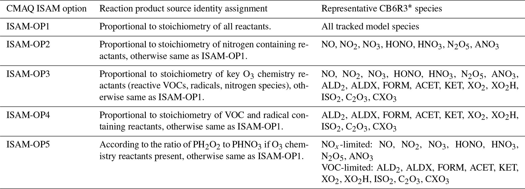
∗ Species are based on CB6R3 and may vary based on different chemical mechanisms implemented in CMAQ. Details can be found in SA_DEFN.F in the CMAQ source code.
2.1 Updates in ISAM
The ISAM implementation in the version 5.0 release of CMAQ was based on Kwok et al. (2013 and 2015). That approach was then updated starting from CMAQ version 5.3 to an attribution based on integrated reaction rates and product yields (U.S. EPA, 2019). The later versions (v5.3.2 and beyond) of CMAQ-ISAM (U.S. EPA, 2022a) employ an apportionment scheme that assigns products of each chemical reaction to sources based on reactant stoichiometry. For example, the isoprene peroxy radical (ISO2) reacts with nitric oxide (NO) to produce several different stable and radical species as represented in the CB6R3 chemical mechanism by the following Reaction (R1).
In addition to nitrogen dioxide (NO2), the products include isoprene nitrate (INTR), formaldehyde (FORM), hydroperoxy radicals (HO2), alkoxy radicals (XO2H), peroxy radicals (RO2), and other isoprene reaction products (ISPD). ISO2 is a product of the oxidation of isoprene, which originates from overwhelmingly biogenic sources. NO is typically emitted from anthropogenic combustion processes, with a much smaller natural component originating from lightning strikes and microbial soil processes on the global scale (Jacquemin and Noilhan, 1990; Yienger and Levy, 1995). Thus, the reactants are approximately half from biogenic sources and half from anthropogenic sources, so the reaction's products have the same attribution distribution. However, source attribution approaches, both receptor-based approaches (such as PMF) and source-based approaches (such as ISAM), are often used to understand how originally emitted NOx and VOC from particular sources ultimately contribute to model-predicted O3 production. The loss of source identity through processes such as the NOx cycle and the role of organic peroxy radicals from sources not controlling O3 production make it difficult to determine the culpability of emission sources. In the preceding example, the NO2 produced by Reaction (R1) is assigned a source that is approximately 50 % biogenic and 50 % anthropogenic. These source assignments propagate quickly when catalytic processes cause NO2 to cycle back to NO through photooxidation and radical oxidation. Because NOx cycling is fast in regional air pollution models, anthropogenically emitted nitrogen species can be assigned to biogenic (or other nearby) sources downwind, so the original source identity was not retained. Reaction (R1) is just one example that illustrates the complex relationship between precursors and subsequent source identities of secondary pollutants. Many such reactions exist in modern chemical mechanisms. Some source apportionment applications, such as O3 source attribution assessments, focus on how sources induce O3 production above background levels. Nitrogen molecules should then retain their original source signatures. This approach is used by other apportionment models such as OSAT, earlier ISAM implementations (Kwok et al., 2015), and other tagging methods (Butler et al., 2018; Grewe et al., 2010).
Because attribution objectives may vary based on scale (e.g., global compared to urban) or purpose (e.g., policy or tracing chemical reactions), ISAM has been enhanced to provide additional configuration options for the user to define how secondarily formed gaseous species are assigned to sources of parent reactants (Table 1) (U.S. EPA 2022b). The existing scheme based on stoichiometrically proportional product attribution introduced in CMAQ version 5.3.2 has been retained as ISAM option 1 (ISAM-OP1). Four new options have been added so the user can configure their simulation based on the application's goal. Each option allows for greater retention of source identity based on subsets of species in the chemical mechanism. ISAM-OP2 apportions products according to the source identity of reactive nitrogen species, including NO, NO2, nitrate radical (NO3), nitrous acid (HONO), HNO3, dinitrogen pentoxide (N2O5), and aerosol nitrate (ANO3). For example, CB6R3 contains the following reaction between the methyl peroxy radical (MEO2) and NO:
In the original ISAM-OP1 configuration, the products of Reaction (R2), FORM, HO2, and NO2 inherit source identities proportional to the source identities of the reactants (MEO2 and NO). However, ISAM-OP2 apportions the product to be from the source identity of NO (presumed predominantly anthropogenic) because NO is a weighted nitrogen-containing species. When a reaction's reactants do not include any of the weighted species, products are apportioned to source identities using the same methodology used in OP1.
ISAM-OP3 expands OP2's list of weighted species to include VOC species identified as important to O3 production. In CB6R3, this includes aldehydes (ALD2 and ALDX), FORM, acetone (ACET), lumped ketones (KET), peroxy operators (XO2 and XO2H), ISO2, acetyl peroxy radicals (C2O3 and CXO3). Therefore, products of reactions containing these VOCs in addition to the nitrogen species of OP2 as reactants would inherit these species' source identities. For example, ALD2 reacts with the NO3 as follows in CB6R3.
The reaction's products, C2O3 and HNO3, inherit identities equally divided between the sources of the reactants because ALD2 and NO3 are on the list of OP3 species. Reactions without any of these species in the reactants list, like OP2, have their products apportioned to source using OP1's methodology when the reactants are not among the weighted ones.
ISAM-OP4 lists only VOC species and daughter products instrumental in O3 chemistry as defined in OP3. In the R1 example, the products are apportioned to the source identity of ISO2 because the other reactant, NO, is not on the list of weighted species. Similarly, the products of Reaction (R3) are attributed to the source identity of ALD2. As in options 2 and 3, reactions (such as Reaction R2) without any listed species are attributed as in OP1's method.
Finally, ISAM-OP5 was added to account for the instantaneously calculated O3 formation regime or limiting case. The regime is determined using the ratio of . The transition point between regimes has a default value equal to 0.35 (Sillman, 1995). For the NOx-limited regime ( > 0.35), source identity is passed from the nitrogen species of OP2, while for the VOC-limited regime ( ≤ 0.35) source identity is passed from the organics of OP4. These CMAQ-ISAM options, including the regime threshold value (or transition point), are accessible at runtime through the standard model run script.
2.2 OSAT description
The source apportionment approach implemented in CAMx is briefly recapped here. Detailed updates of all OSAT versions can be found in the CAMx official user guide (https://camx.com/Files/CAMxUsersGuide_v7.10.pdf, last access: 1 February 2023). All available versions of OSAT (including OSAT3) in CAMx separately solve for production and destruction of O3 with production being attributed to either NOx or VOC emissions, depending on which is estimated to be limiting O3 production. When the ratio of exceeds 0.35, the produced O3 is attributed to NOx emissions, and VOC emissions below that threshold. The CAMx source apportionment implementation includes an option (OSAT-APCA) that allows for a redirection of attribution to anthropogenic emissions in situations where the limiting precursor is biogenic. In CAMx-OSAT, O3 attributed to NOx and VOCs is tracked as separate tracer groups. O3 tracers are first adjusted to account for O3 destruction processes and subsequently for net O3 production, which is defined as the difference between O3 production and O3 destruction based on a subset of photochemical reactions that result in O3 destruction. In situations where the net O3 production is negative (destruction reactions dominate), all the O3 tracers are proportionally decreased. When net O3 production is positive, production is assigned proportionally to the sources of those emissions (NOx and VOC precursor tracers) at the time and place where O3 was made. OSAT includes a group of tracers that track odd oxygen that is consumed when O3 reacts with NO to form NO2 that can quickly photolyze and reform O3 through a reaction with oxygen. In this situation, the O3 removed from the O3 tracers due to the NO + O3 reaction is moved to the odd-oxygen tracers (which have separate NOx and VOC tracer groups). When NO2 is photolyzed and O3 formed, a proportional amount of O3 is taken from the odd-oxygen tracers and moved to the O3 tracers.
Table 2CMAQ and CAMx model configurations
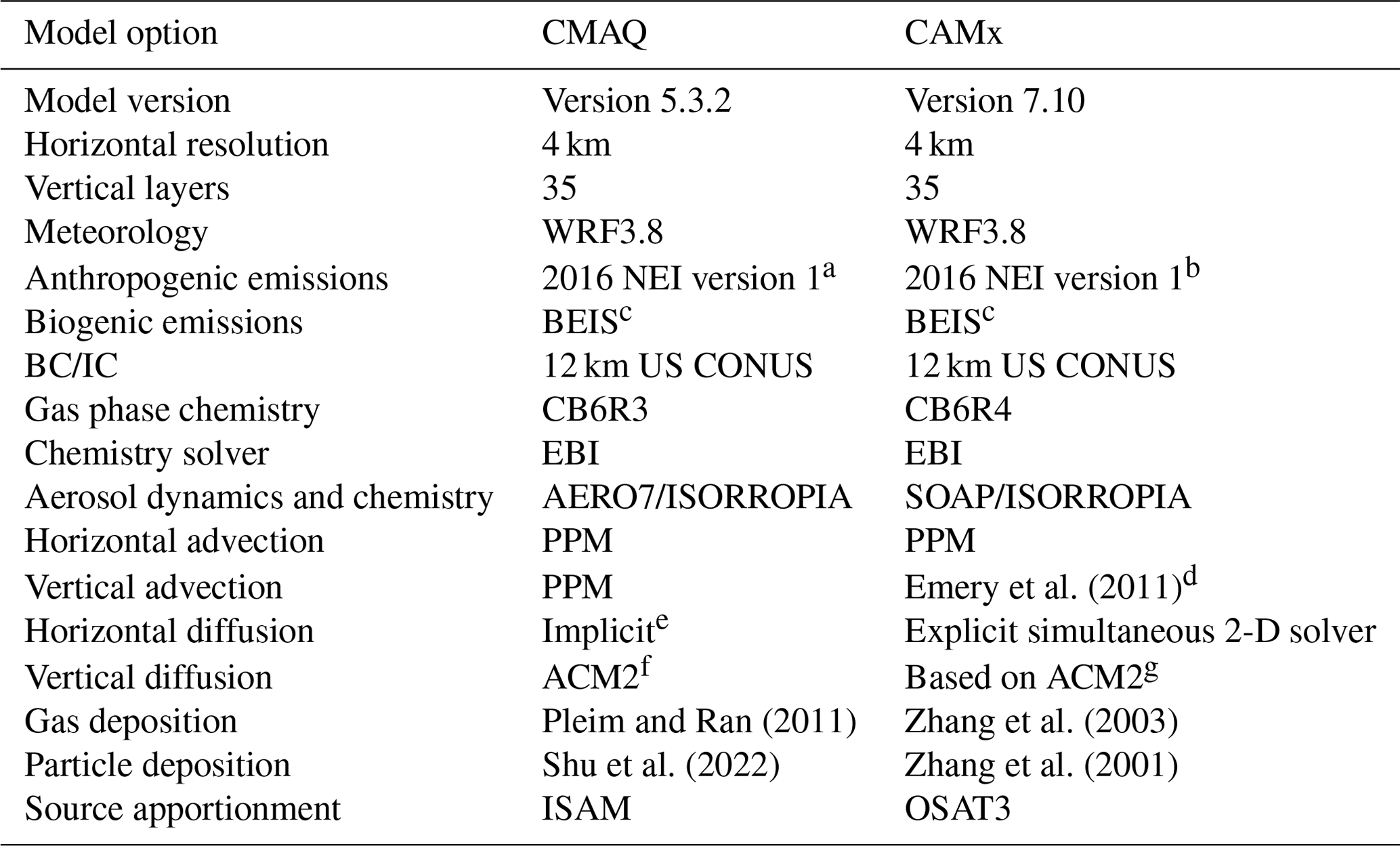
a EGUs were based on continuous emissions monitoring data from 2018 where available. On-road emissions were projected to 2018. b CAMx EGU and on road were identically processed as CMAQ. c BELD v4.1 vegetation data for biogenic emissions, and the BEIS version is 3.61. d Backward Euler (time) hybrid centered and upstream (space) solver. e Horizontal diffusion fluxes for transported pollutants were parameterized using eddy diffusion theory. The horizontal diffusivity coefficients were formulated using the approach of Smagorinsky (1963). f KZMIN was turned on in CMAQ as default. g Vertical diffusivity coefficients were calculated with Yonsei University (YSU) bulk boundary layer scheme (Hong et al., 2006) and were adjusted with the KVPATCH, which is comparable to the KZMIN approach in CMAQ.
3.1 Base model configurations
Two models, CMAQ version 5.3.2 with modified ISAM and CAMx version 7.10 with OSAT3, are used to simulate a 1-month period during the summer of 2018 (29 July to 30 August). The summary of the two model configurations is presented in Table 2. Both models are applied to the same horizontal modeling domain with 4 km × 4 km resolution encompassing the northeastern US. This domain is nested within a larger 12 km domain that encompasses the entire contiguous United States, which is used for providing simulation boundary and initial conditions (BCs and ICs) for the 4 km domain. BCs were generated for the 12 km simulations using a hemispheric application of the GEOS-Chem model (Henderson et al., 2014) that was run for 2018. Identical ICs and BCs were applied to the two models. Anthropogenic emissions were based on version 1 of the 2016 National Emission Inventory (NEI, U.S. EPA, 2021). Electrical generating unit emissions were based on continuous emissions monitoring data from 2018 where available. On-road emissions were projected to 2018 to reflect decreases in emissions due to vehicle fleet turnover and the implementation of emission control technology in 2017. The Biogenic Emission Inventory System (Bash et al., 2016) was used to generate biogenic volatile organic compound emissions, and offline meteorology was created using the Weather Research and Forecasting (WRF, Skamarock et al., 2008) model version 3.8. CMAQ was configured using Carbon Bond 6 version 3 (CB6R3, Emery et al., 2015) for chemistry. Similarly, all base meteorological and emissions inputs for CAMx were identical to those for CMAQ but were processed using CAMx-appropriate data pre-processors (https://www.camx.com, last access: 10 March 2021). The CAMx model was configured with Carbon Bond 6 version 4 (CB6R4, Emery et al., 2016a) chemical mechanism. It is noteworthy that the major updates for CB6R4 from CB6R3 are to (i) replace full marine halogen chemistry with a condensed iodine mechanism called “I-16”, which could reduce O3 depletion over marine areas, and (ii) add dimethyl sulfide (DMS) chemistry. Emery et al. (2016b) demonstrated that the difference in O3 decrements between full halogen chemistry and I-16 is small and can be neglected over land.
3.2 Source apportionment simulation designs
As discussed in Sect. 2, ISAM has been updated to include a user option with five possible configurations for source apportionment approach. Here, we conduct CMAQ source apportionment simulations for all these options: ISAM-OP1, ISAM-OP2, ISAM-OP3, ISAM-OP4, and ISAM-OP5, hereafter referred to as OP1, OP2, OP3, OP4, and OP5, respectively. The OSAT3 approach was also used in the CAMx v7.10 base model for comparison with the five ISAM simulations. Hereafter OSAT3 is referred to as OSAT. A brute-force method (zeroing out the entire emission stream for tracked sources in CMAQ, hereafter referred to as CMAQ-BF) was also used to compare with the ISAM options and OSAT. A total of 11 different emission source categories were tracked using each apportionment technique. The source categories comprise four point source categories, including electricity generating units (EGU), non-electricity generating units (NONEGU), fires (FIRE), and commercial marine vessels (CMVs), and six area-source categories, including on-road mobile (ONROAD), non-road mobile (NONROAD), biogenic (BIO), railway (RAIL), airports (AIRP), and other sources (AREA). Additionally, OILGAS was tracked as a mixed category (both point and area) of emissions from the oil and natural gas industry in the domain. Total emissions from the above sectors have been displayed in Table 3. Finally, three predefined tracers for lateral boundary conditions (BCON), initial conditions (ICON), and other sources (OTHR) were also tracked for O3 and its precursors. OTHR is used for all remaining untagged emission categories. For example, when there are a total of 10 emission streams but only 5 of them are tracked in ISAM, the remaining 5 emission streams will be defined as OTHR. In this study, all emissions sectors were tracked as previously mentioned above for OSAT and ISAM. For CMAQ-BF, a unique CMAQ simulation for each emission source category listed above was performed by fully removing the category's entire emission stream. CMAQ-BF apportionment was then calculated by subtracting the resulting pollutant fields from a base model simulation. However, for ICON and BCON, each was reduced by 50 % and the output field difference with the base model was scaled up by a factor of 2 to avoid numerical issues associated with very low model ICON and BCON values. As for OTHR, there is no suitable way to retain an appropriate chemical state of the troposphere after subtracting necessary emission categories, initial and boundary conditions from an original CMAQ simulation. Thus, OTHR is not being compared among CMAQ-BF, ISAM, and OSAT in this study.
Table 3Total emissions from each sector for the 4 km northeastern US domain (month of August 2018).
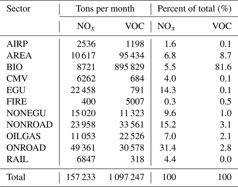
Table 4Tracked species classes between ISAM and OSAT.
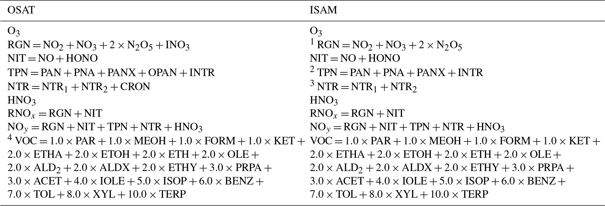
1 ISAM does not track INO3. 2 ISAM does not track OPAN. 3 ISAM does not track CRON. 4 OSAT VOC has been pre-calculated as an equation in Table 4.
3.3 Tracked species classes
O3, NOx, and VOC species were tracked by each method. As mentioned above, ISAM tracks individual oxidized nitrogen and VOC species based on selected chemical mechanisms in CMAQ, whereas OSAT tracks tracer families for each. To facilitate the comparison between the two models, the ISAM species were aggregated in the same fashion as OSAT (Table 4). However, some differences still exist since species representations between the two models are not completely the same. The nitrogen groupings NOy and RNOx (Table 4) were added to better elucidate the behavior of each model under different O3-producing chemical regimes.
3.4 Evaluation method and case study development
Although identical emissions and meteorological inputs are used for CAMx and CMAQ (Table 2), potential differences still exist in multiple scales and processes. Shu et al. (2017, 2022) have reported that deposition is one of the largest uncertainties between the two models when other processes are constrained. For inter-comparing ISAM and OSAT, it is not feasible to constrain all process uncertainties. Thus, we established criteria to choose representative days for ISAM and OSAT comparisons based on the performance of their parent models rather than comparing them throughout the entire simulation period to reduce the difference that may be brought on from their parent models. We initially set the correlation relationship (R2) criteria of maximum daily 8 h averaged (MDA8) O3 between CMAQ and CAMx to be above 0.7 to ensure that the performance of the two parent models is comparable. Next, MDA8 O3 was also used as the indicator for case study selection since ISAM and OSAT are normally used as regulatory application with this metric. We assess the mean bias (MB) of MDA8 O3 for every day to choose the days on which both models have the lowest MB for predicted MDA8 O3. Therefore, CMAQ- and CAMx-simulated ambient concentrations were paired in space and time with observed data from the Air Quality System (AQS, https://www.epa.gov/aqs, last access: 9 June 2021) monitoring network. Hourly concentrations of total O3, NO and NO2 were also compared to the AQS observations, and their bias statistical metrics were calculated as well.
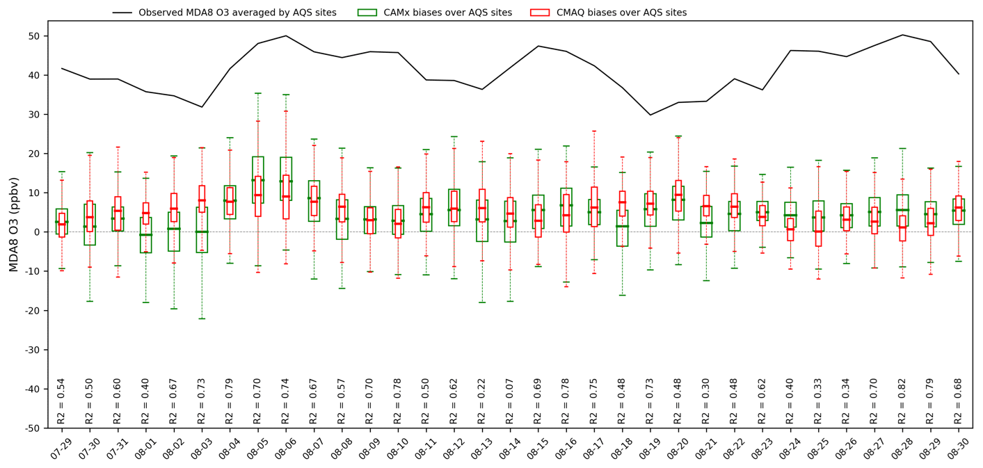
Figure 1Observed site-averaged MDA8 O3 and its corresponding biases predicted by CMAQ and CAMx over paired AQS sites for the entire episode. R2 shows the correlation relationship between CMAQ and CAMx.
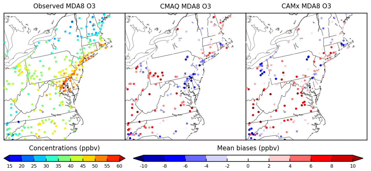
Figure 2The 2 d averaged observed MDA8 O3 over paired sites for the northeastern US domain and its corresponding mean biases predicted by CMAQ and CAMx for the selected case study.
Table 5Model performance summary at paired AQS surface monitoring sites. (monthly episode).

a Mean bias is . MB ranges from negative infinity to positive infinity with 0 indicating unbiased data, and the unit here is ppbv. b Normalized mean bias is , and this ranges from negative 1 to positive infinity with 0 indicating unbiased data. The values shown in the table were multiplied by 100. c Root-mean-square error is , and this is the standard deviation of the prediction errors. d . R2 ranges from 0 to 1, with 1 indicating perfect correlation and 0 indicating an uncorrelated relationship.
Table 6Model performance summary at paired AQS surface monitoring sites. (2 d case study episode)
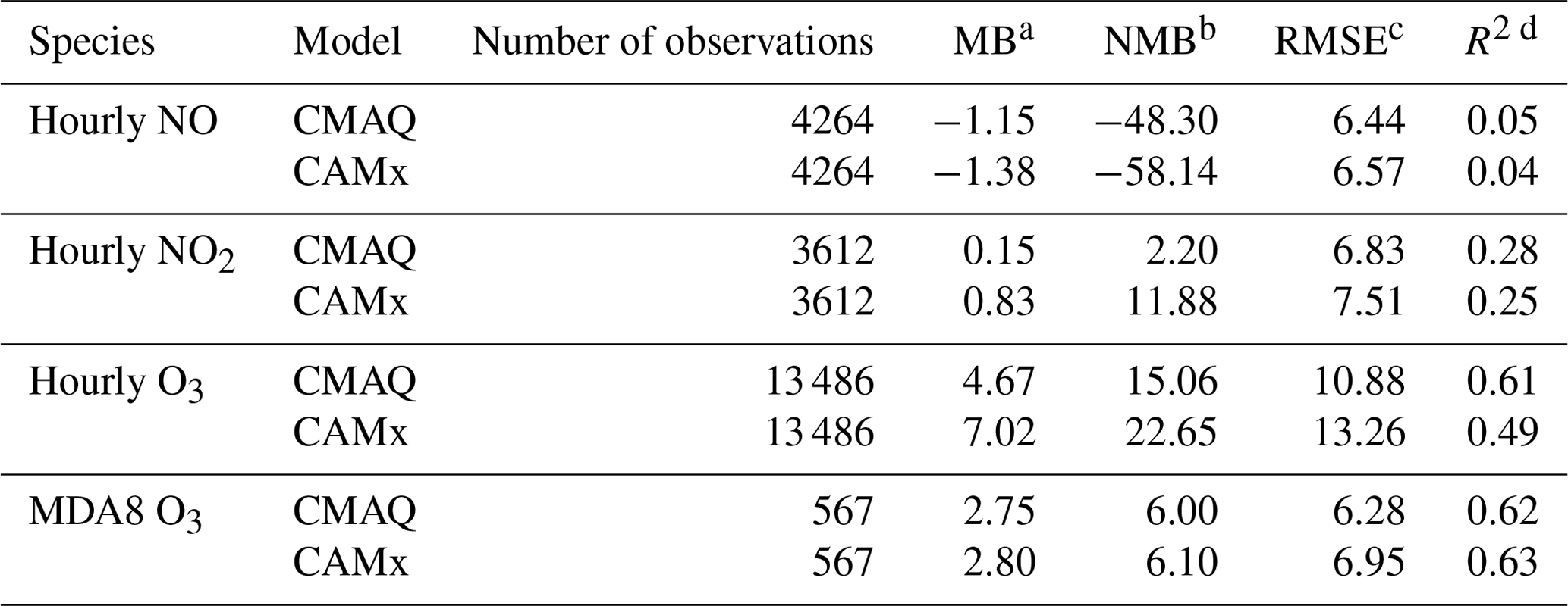
a Mean bias is . MB ranges from negative infinity to positive infinity with 0 indicating unbiased data, and the unit here is ppbv. b Normalized mean bias is , and this ranges from negative 1 to positive infinity with 0 indicating unbiased data. The values shown in the table were multiplied by 100. c Root-mean-square error is , and this is the standard deviation of the prediction errors. d . R2 ranges from 0 to 1, with 1 indicating perfect correlation and 0 indicating an uncorrelated relationship.
4.1 Model performance evaluation and case study selection
Figure 1 shows observed site averaged MDA8 O3 and its corresponding biases predicted by CMAQ and CAMx over paired AQS sites for the entire episode. Observed site averaged MDA8 O3 ranges from 30 to 50 ppbv. The performance of two models for predicting MDA8 O3 varies by paired day and monitor site with the range of biases from −23 to 35 ppbv, approximately. Table S1 in the Supplement summarizes R2 and MB of MDA8 O3 for each day for both models. Based on our criteria introduced in Sect. 3.4, there are 13 d on which the two models show very good correlation relationships. Among these days, two models both show good performance on predicting MDA8 O3 with closest MB on 9 August (CMAQ/CAMx = 3.09/2.99 ppbv) and 10 August (CMAQ/CAMx: 2.42/2.61 ppbv). For other days, either two models both have higher MB (> 10 ppbv), or their predictions do not agree well with each other, with a difference of MBs up to 8 ppbv. Therefore, 9 and 10 August were selected as a 2 d case study for source apportionment comparisons. Additional evaluations of hourly O3, NO and NO2 is available in Fig. S1 in the Supplement. From Fig. 2, MDA8 O3 is relatively higher over east coastal urban areas with generally over 50 ppbv but reduces to 35 ppbv at other rural areas of northeastern US domain. The two models predicted MDA8 O3 show very good agreement spatially, underestimating MDA8 O3 at sites where observed MDA8 O3 is high but overestimating MDA8 O3 at sites where O3 is low. Similar spatial plots of hourly paired O3, NO and NO2 can be found in the Supplement (Fig. S2). Tables 5 and 6, respectively summarize statistical metrics for MDA8 O3, hourly O3, NO and NO2 at all paired monitoring sites for the monthly O3 episode and the selected 2 d case study episode.
The metrics in Tables 5 and 6 both show consistent results with Fig. 1 as discussed above. The changes of NO and NO2 metrics are marginal from the monthly episode to the 2 d case. As in Fig. S1, NO and NO2 concentrations are less variable than O3 across days in the monthly episode, as a result, the comparison of NO and NO2 are less dependent on which day is selected. Unlike NO and NO2, CAMx and CMAQ performance is statistically better in the 2 d case study with lower MB for hourly O3 (CMAQ/CAMx = 4.67/7.02 ppbv) and MDA8 O3 (CMAQ/CAMx = 2.75/2.80) than the monthly episode (hourly O3: CMAQ/CAMx = 6.49/7.99 ppbv; MDA8 O3: CMAQ/CAMx = 5.30/4.18). The differences of MB, NMB and R2 between the two models also diminish for MDA8 O3 but increase for hourly O3 from the monthly episode to the 2 d episode. The statistical metrics of hourly O3 and MDA8 O3 demonstrate that the selected 2 d case is suitable for a source apportionment comparison in which CAMx and CMAQ not only both have the least-biased predictions compared to observations but also show a good agreement with each other.
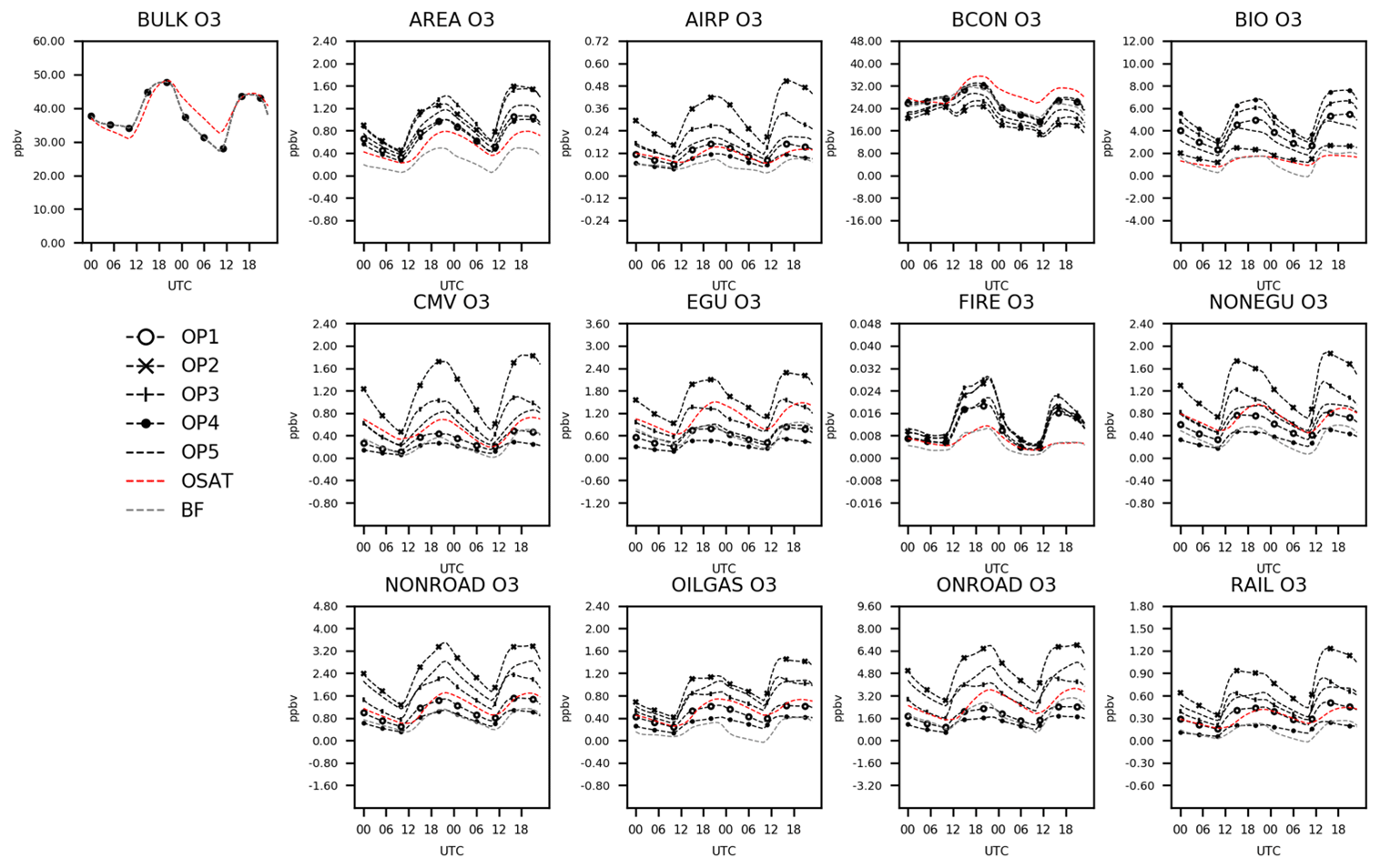
Figure 3Total and attributed O3 concentrations to various sectors as a function of hour of day and apportionment technique.
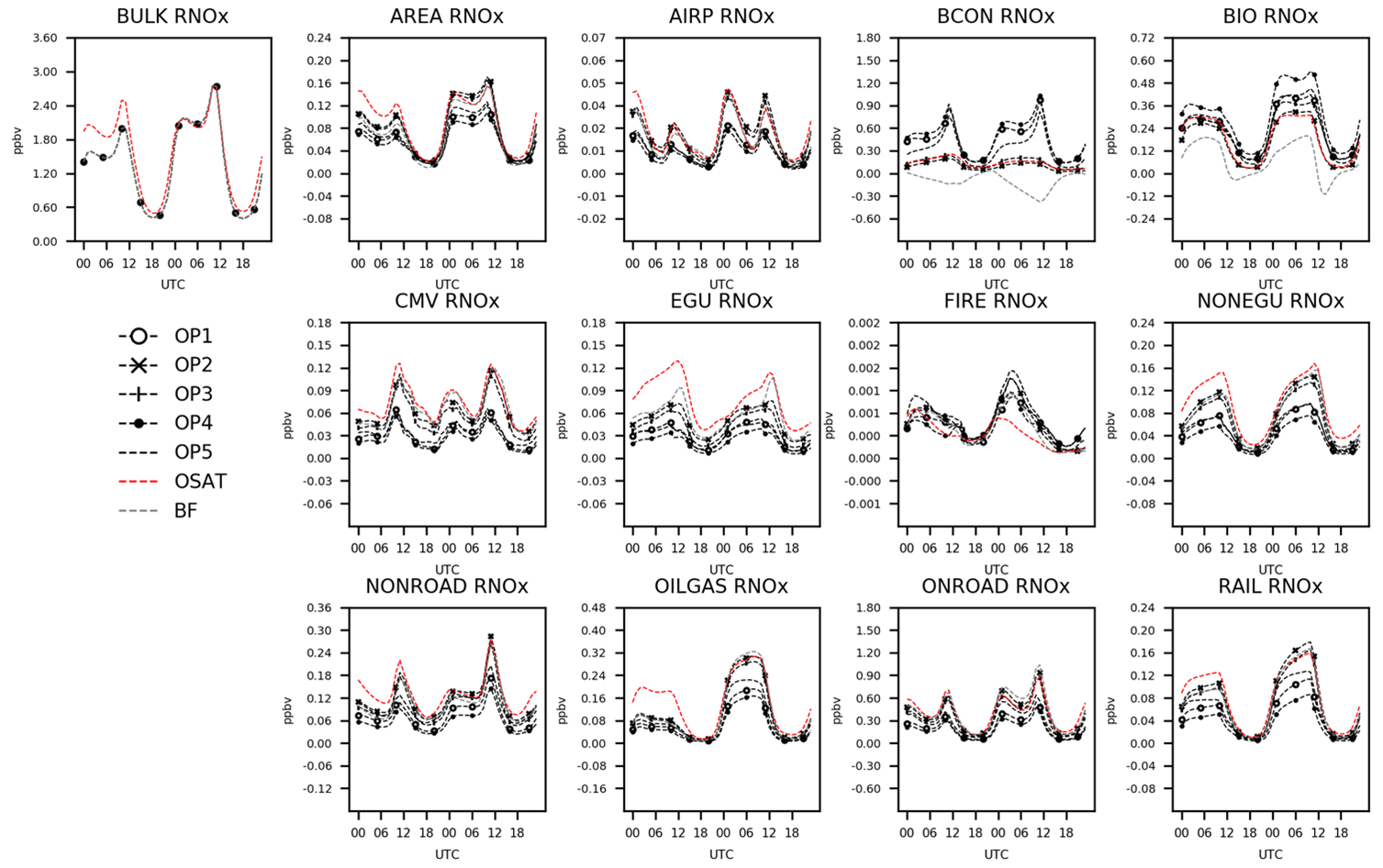
Figure 4Total and attributed RNOx concentrations to various sectors as a function of hour of day and apportionment technique.
4.2 Comparison of model source apportionment
4.2.1 Temporal variations of sector contributions
To better understand how the ISAM model apportionment approach simulated source contributions at each time step, time series comparisons for each source were examined for O3 and its precursors, RNOx, and VOC for the 2 d case study. Figure 3 shows hourly variations of domain averaged predicted total O3 (bulk) concentrations and sector contributions for seven source apportionment simulations (OSAT, BF, ISAM OP1 to OP5). In Fig. 3, CMAQ and CAMx predict similar O3 concentrations during the day, but differences appear at night, with a maximum difference of 5 ppb. This disparity was discussed in Sect. 4.1 and can be mitigated by employing the MDA8 O3 metric. The seven source apportionment simulations yield similar diurnal trends via the trajectory of the total concentrations, but they apportion concentrations to each sector somewhat differently. Comparisons of five ISAM options reveals significant variability. OP1, which apportions uniformly according to stoichiometry, shows similar trends of apportionments for each sector as OP4, an option that always allocates products to sources with reactive VOCs and their radicals. They both apportion more BCON and BIO O3 but fewer contributions from all other sectors than the other three ISAM options (OP2, OP3, and OP5). Results of OP1 and OP4 would likely overestimate sensitivity to emissions to these reactants because VOCs are often available in excess. OP2 always allocates products to sources with nitrogen reactants, which prevents the attribution of NOx to non-nitrogen reactants. Typically, these non-nitrogen reactants are common in transported (e.g., BCON) or natural sources (e.g., isoprene in BIO). As a result, OP2 decreases BCON and BIO contributions while increasing contributions from other sectors relative to OP1 and OP4.
OP5 assigns products to either reactive VOCs or NOx based on the ratio of , placing O3 contribution results for all sectors between the previous four ISAM options. OSAT, which utilizes a similar methodology to OP5, shows consistent diurnal patterns of domain averaged total O3 and sector contributions compared to the ISAM options but with varying magnitudes. OSAT has the largest BCON O3 but the lowest contributions from AREA, BIO, and FIRE. The rest of the OSAT sector contributions are between the ISAM options. Consistent with earlier findings, CMAQ-BF estimates systematically smaller O3 contributions for all sectors besides EGU and BCON (Kwok et al., 2015). While ISAM and OSAT appear to retain bulk mass as intended, CMAQ-BF shifts the chemical system into a different nonlinear O3 response to source change.
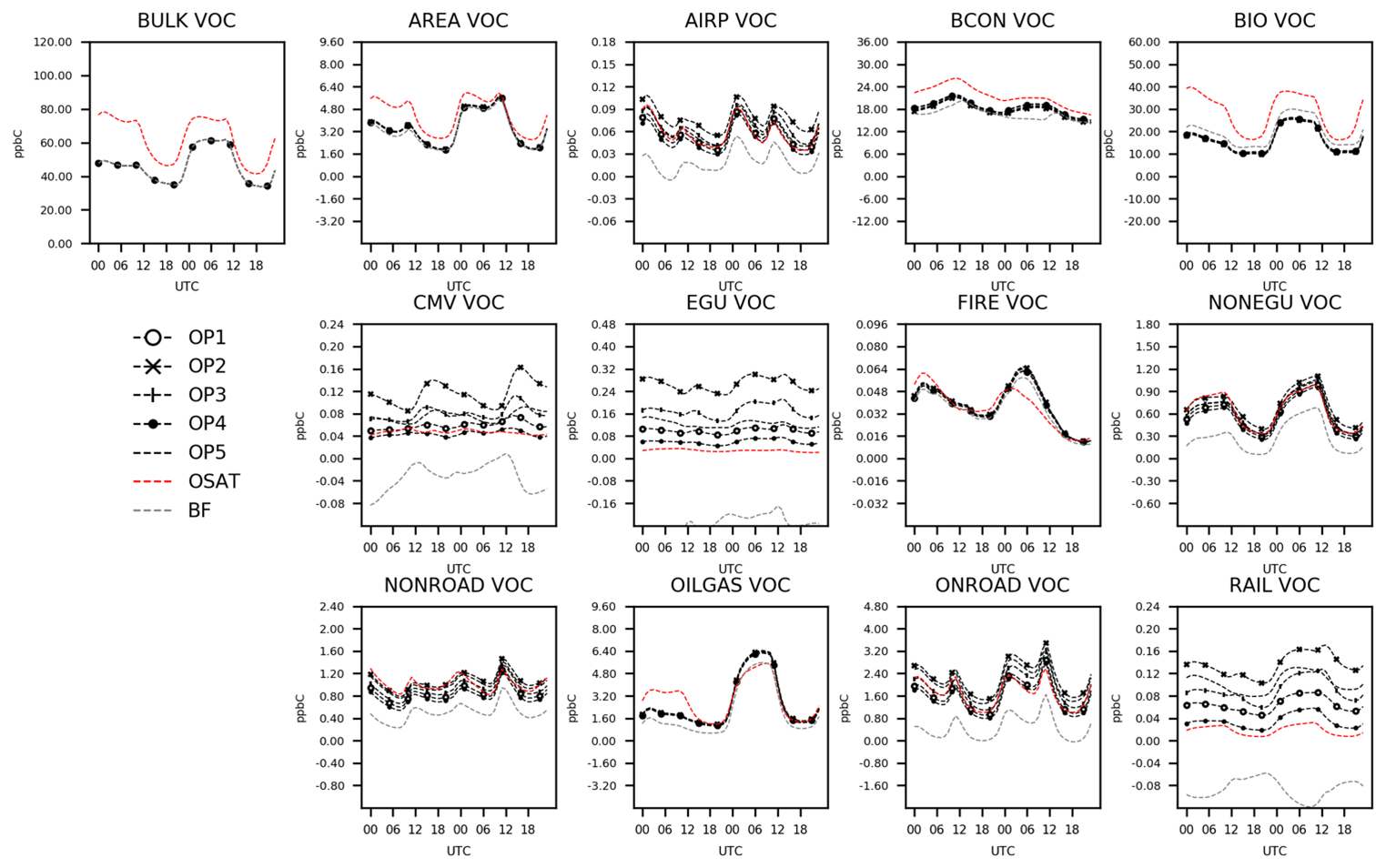
Figure 5Total and attributed VOC concentrations to various sectors as a function of hour of day and apportionment technique.
In Fig. 4, CAMx and CMAQ predict comparable total RNOx except for the first 12 h of the 2 d example, when OSAT values deviate from those of the other six simulations. As the total concentrations of the two models converge, OSAT exhibits similar patterns to OP2 and OP3. OP1, OP4, and OP5 show comparable results, with increased BCON and BIO RNOx but decreased contributions from other sectors. CMAQ-BF show comparable results with OSAT, OP2, and OP3 except for BCON and BIO, which are negative for CMAQ-BF, suggesting that removing these source sectors results in a slight rise in RNOx. In previous source sensitivity and allocation investigations, it has been shown that BF may have limits when the model response contains an indirect effect coming from the influence of substances other than the direct precursors (Kwok et al., 2015; Burr and Zhang, 2011; Koo et al., 2009; Jiménez, 2004; Zhang et al., 2009). This would be particularly true in situations where emissions are a large percentage of total NOx or VOC in a particular area. The nonlinear impacts on gas-phase chemistry realized in a source sensitivity model simulation would not be a relevant representation of culpability from that same source group.
Figure 5 illustrates the hourly variability of domain-averaged VOC concentrations and sector contributions. CAMx only gives pre-lumped VOC (Table 4) for OSAT outputs. For consistency, VOC for CMAQ ISAM and BF has also been carbon-weighted by summing all individual VOC species in CMAQ outputs using the same method as OSAT (Table 4). In Fig. 5, CAMx consistently simulates higher attribution to total VOC concentrations than CMAQ, with a maximum difference of 30 ppb. These larger CAMx VOC concentrations are also reflected in apportioned OSAT sectors, particularly those with substantial contributions, such as BCON and BIO. Given that the difference is present in the total concentration, this is unlikely caused by different source apportionment formulation between CMAQ and CAMx. As CAMx only gives pre-lumped VOC, it is challenging to compare individual VOC species between CMAQ and CAMx to explain this difference at current stage. Another possible reason for this could be that models have different internal treatments for advection and diffusion, which can impact surface-level concentrations and indirectly impact chemical reactions. The five ISAM options have comparable diurnal patterns for most sectors, with the exception of CMV, EGU, and RAIL; however, the magnitudes for these three sectors are relatively minor, which is consistent with earlier findings (Kwok et al., 2015). CMAQ-BF estimates notably lower sector contributions for VOCs, which is similar to O3 results (Fig. 4), with negative contributions for small sectors (e.g., CMV, EGU, and RAIL). Additional figures of other grouped nitrogen species tracked in Table 4 (e.g., RGN, HNO3, and NOy) can be found in the Supplement.
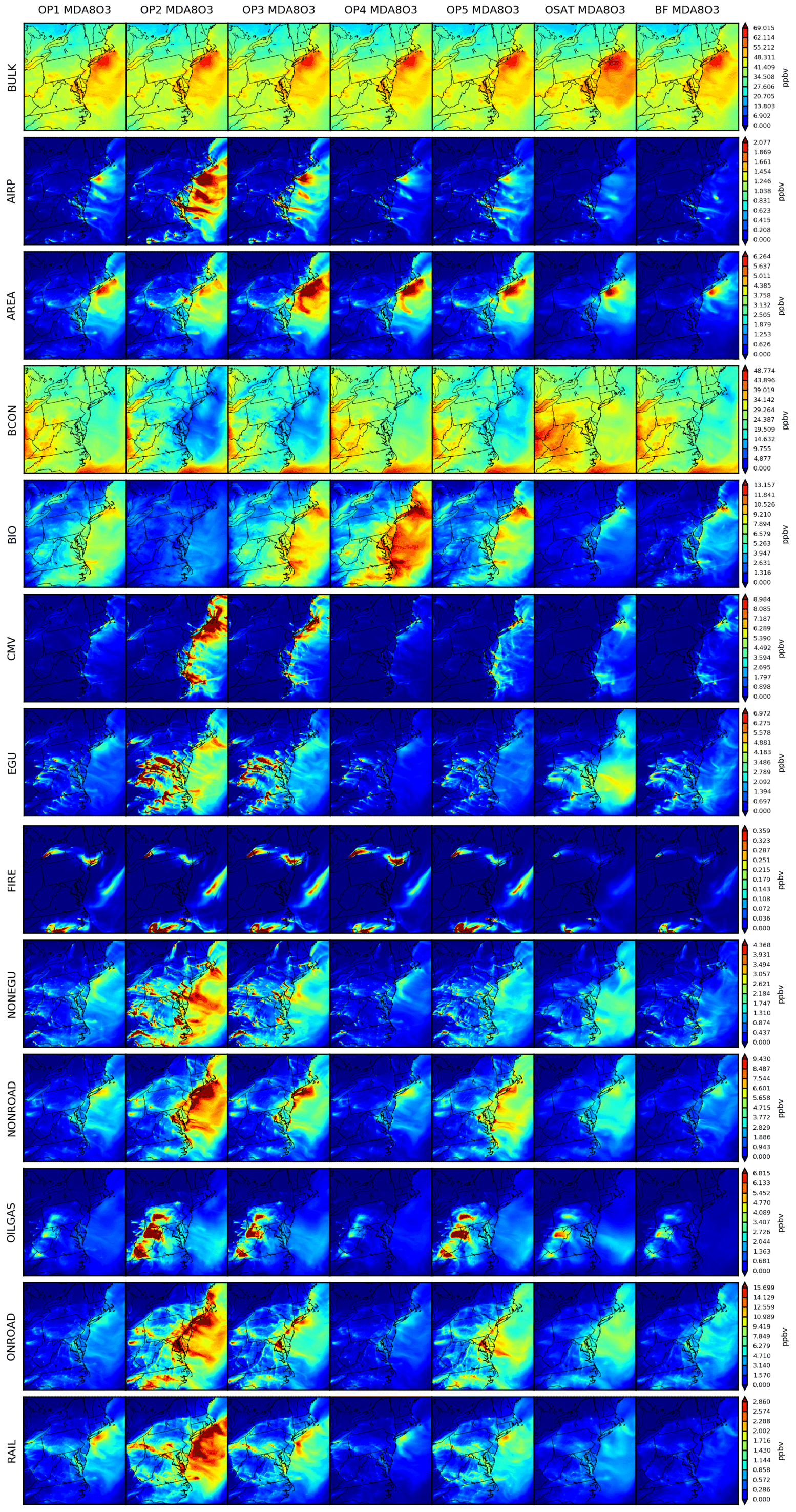
Figure 6Spatial comparisons of seven simulations for 2 d averaged O3 (9 and 10 August).
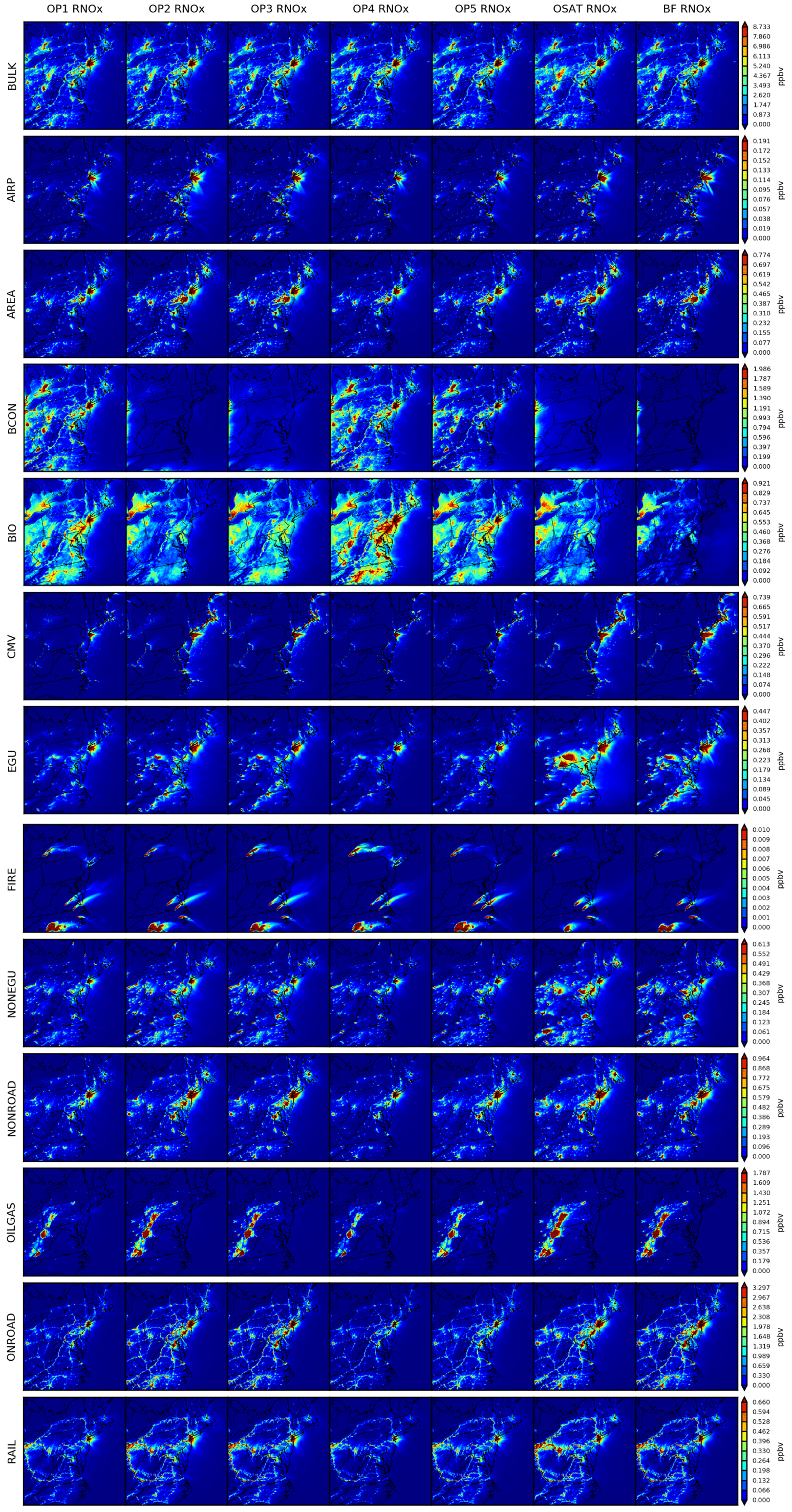
Figure 7Spatial comparisons of seven simulations for 2 d averaged RNOx (9 and 10 August).
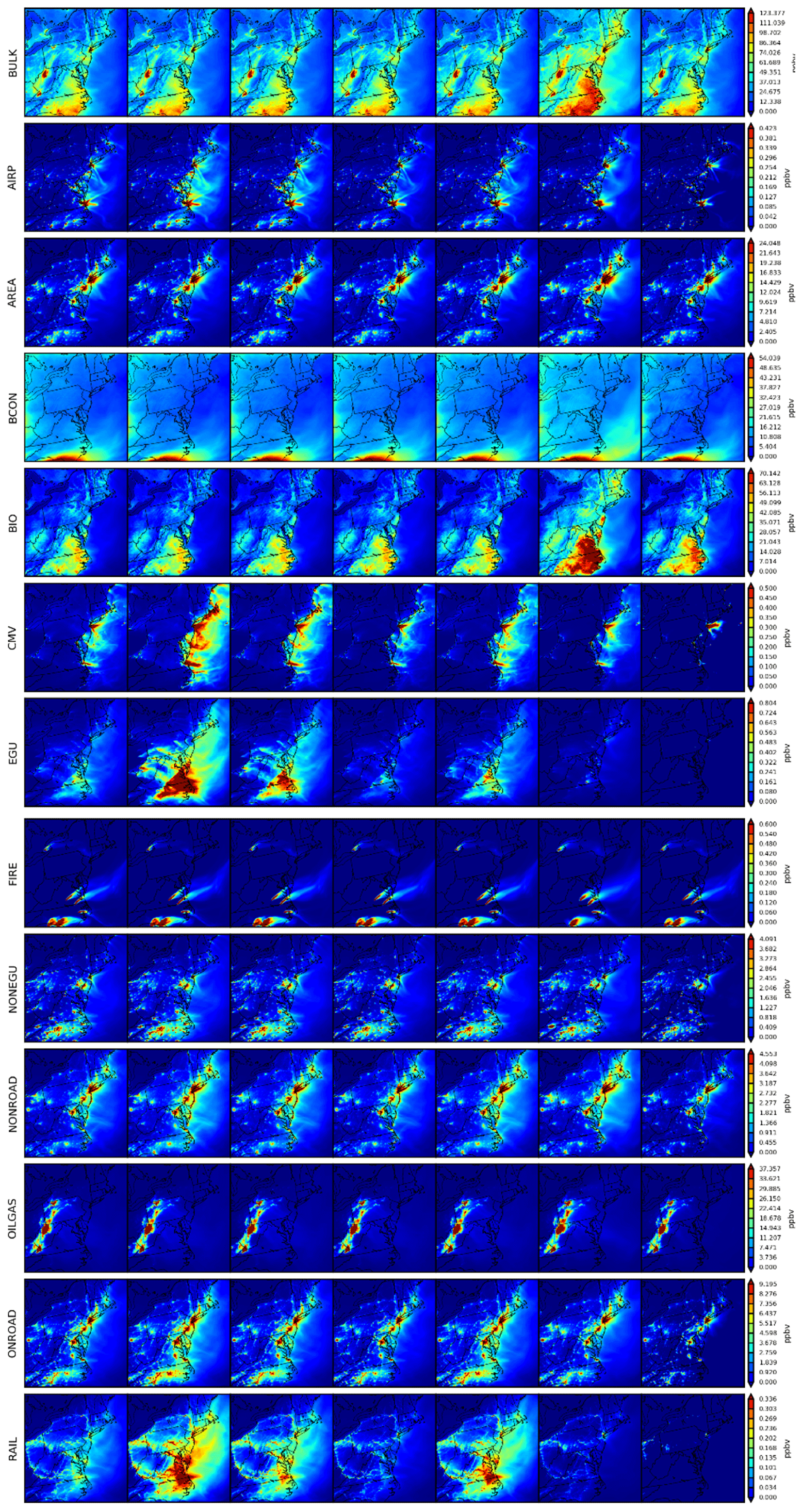
Figure 8Spatial comparisons of seven simulations for 2 d averaged VOC (9 and 10 August).
4.2.2 Spatial distribution of source apportionment simulations
Spatial patterns of total and sector contributions of MDA8 O3 (Fig. 6), RNOx (Fig. 7) and VOC (Fig. 8) have been examined for the seven simulations. In Fig. 6, OSAT exhibits the same spatial distribution of MDA8 O3 total concentrations as other CMAQ-based simulations (OP1, OP2, OP3, OP4, OP5, and CMAQ-BF), with the exception of OSAT's relatively high marine and offshore total concentrations (> 5 ppbv), which could be explained by the difference in planetary boundary layer dynamics or different marine chemistry configuration between the two parent models. CMAQ CB6R3 uses a rough parameterization for full marine halogen chemistry to destroy O3, depending only on land-use category and sunlight (Sarwar et al., 2015, 2019), whereas CAMx CB6R4 handles O3 depletion in the marine boundary more efficiently by including the 16 most important reactions of inorganic iodine (I-16b, Emery et al., 2016b). According to a sensitivity test conducted by Emery et al. (2016b), I-16b could reduce O3 depletions by 2–5 ppbv in comparison to full halogen chemistry. Regarding sector concentrations, the spatial distributions of seven simulations are comparable. They can all capture geographic contribution hot spots from each sector, although their magnitudes vary. OP2 stands out with fewer contributions from BIO than the other four ISAM options, and subsequently assigns larger concentrations to other sectors, particularly over east coastal regions, as shown in Figs. 3 and 6. Since OP2 assigns all products to sources with nitrogen reactants, the influence of reactants from biogenic sources is diminished, as intended.
Figure 7 depicts the associated outcomes of RNOx. Except for BCON, the seven simulations produce geographically and quantitatively consistent findings. From the spatial distributions, we can conclude that local sources govern RNOx more than long-transported sources compared to O3. Anthropogenic RNOx is either more concentrated in the urban areas (e.g., AREA, NONEGU, NONROAD), gasoline industry (OILGAS) and electric facilities (EGU) or along with transportation (e.g., AIRP, ONROAD, CMV and RAIL). Biogenic RNOx is more prevalent in rural locations with vegetation. It should be noted that OP1, OP4, and OP5 show more BCON RNOx across the entire domain because of the method used to assign products in nitrogen-related reactions (Sect. 2). OP1, OP4, and OP5 show local hotspots of RNOx attributed to BCON. Since there is no physical reason to suspect hotspots over urban areas, we conclude that these contributions represent RNOx attributed based on VOC or oxidants transported from the boundary. Figure 8 depicts the outcomes associated with VOC. Higher VOC concentrations from CAMx already shown in Fig. 5 are primarily from Virginia and North Carolina (OSAT bulk). As CMAQ and CAMx both use the same BEIS inventory data, the difference in total VOC concentrations may result from other differences between two models, like chemistry or deposition, accordingly leading to higher biogenic sources in CAMx (BIO). For the rest of the sectors, OSAT and ISAM options are fairly consistent except that the OP2 predicts more contributions from EGU, CMV, and RAIL. CMAQ-BF predicts consistently lower source contributions for MDA8 O3, RNOx, and VOC, as shown in Sect. 4.2.1. This yet again illustrates that brute force represents an integrated sensitivity while the OSAT and ISAM represent attribution at a point in the nonlinear chemical systems. Monthly averaged spatial maps for MDA8 O3, RNOx, and VOC are also included in Fig. S4a–c in the Supplement and show consistent results as 2 d averaged maps. This demonstrates that our case study is appropriate, efficiently selecting representative days as well as minimizing the uncertainties from parent models (CMAQ and CMAQ). Additional figures of other grouped nitrogen species tracked in Table 4 (e.g., RGN, HNO3 and NOy) can also be found in the Supplement.
The CPU time required to complete a source apportionment simulation in a 3D AQM is an important consideration for usability. For a 4 km × 4 km simulation domain encompassing the northeastern US, the model run times for OSAT and ISAM are similar. Using 128 processors, base CMAQ (without ISAM) and CMAQ-ISAM simulations (11 source categories) are tested. Base CMAQ requires around 60 min per simulation day (24 h), whereas CMAQ-ISAM requires approximately 120 min. If the number of processors is increased to 256, the simulation time for CMAQ-ISAM can be reduced by 30 min, showing good scalability. It is worth noting that our CMAQ-ISAM simulations simultaneously track all additional species classes, such as sulfate, nitrate, ammonium, elemental carbon, organic carbon, and chloride. It would shorten simulation times if related species were only tracked for O3. Base CAMx (without OSAT) and CAMx OSAT are also tested with 128 processors, taking 37 and 67 min, respectively. CAMx also provides an optional tool for particles that can be simultaneously applied similarly to ISAM (PSAT, Yarwood et al., 2007). When additional pollutants are selected for tracking (e.g., sulfate, primary PM2.5 species) total simulation time will increase for both ISAM and OSAT and/or PSAT. CMAQ-BF speed is based on CMAQ base simulation (60 min d−1 × (1 base + 11 sources + 1 boundary condition + 1 initial condition + 1 other) = 900 min d−1).
Source attribution approaches are generally intended to determine culpability of precursor emission sources to ambient pollutant concentrations. Source-based apportionment approaches such as ISAM and OSAT provide similar types of information, specifically an estimate of which sources or groups of sectors (e.g., a sector) contributed to the air quality measured or estimated at a particular location. The assumptions in each technique have implications for interpretations in the context of air quality management.
Source attribution of secondarily formed pollutants cannot be explicitly measured, which makes evaluation of source apportionment approaches challenging. Here, the ISAM approach was evaluated by (i) a comparison with a source apportionment approach implemented in a different photochemical modeling system and (ii) a comparison with a simple source sensitivity (brute-force difference) approach in the same modeling system that is most comparable to source apportionment in more linear systems and less useful when formation and transport are nonlinear. Further, this section notes qualitative consistency between the spatial nature of sector emission and the attribution of precursors and O3 as another method to generate confidence in these approaches.
In this study, multiple apportionment approach comparisons show common features but still reveal wide variations in predicted sector contribution and species dependency. The attribution to sources emitting NOx and VOC is consistent with the spatial nature of these sources, which provides confidence in the approach. However, nitrogen species (e.g., NOx), for instance, are more sensitive to the choice of ISAM options than VOC. For example, although the attribution of NOx to EGUs matches the location of these sources (e.g., New York urban area) for all ISAM options, OP1, OP4, and OP5 predict more BCON NOx. This is because the fast NOx cycling process assigns anthropogenically emitted nitrogen species to other sources, as the original emitted source identity is not retained through these complex reactions. Further, sources entirely located offshore, such as commercial marine vessels, do not have culpability assigned to distant inland regions of the model domain. Most of the time, the amount of attribution to a certain sector depends on the number of emissions from that sector, how far away those emissions are, and whether the prevailing winds carried emissions from those places to the monitor or grid cell where air quality was predicted.
The five designed ISAM options maximize its flexibility, particularly for modeling source apportionment of O3 and its precursors, but the choice of option depends on target species. Among all ISAM options, the OP5 option, after making the assignment decision based on the ratio of PH2O2 to PHNO3, is expected to predict generally similar spatial and temporal patterns for O3 to the OSAT source apportionment approach implemented in CAMx. However, it still shows disparity for some sectors (e.g., biogenic sectors for O3). This result may be because of the OSAT formulation, which differs from the ISAM options presented here. The OP5 option was also similar to brute-force sensitivity estimates predicted in CMAQ with the exception of source groups that dominate regional emissions or O3, such as biogenic VOC and O3 introduced into the model through boundary inflow. In those situations, it is not reasonable to expect a source sensitivity approach to provide a useful comparison for source attribution given the highly nonlinear change in atmospheric chemistry. After assigning products to sources emitting nitrogen reactants, the OP2 option can predict results of RNOx attributions that are more comparable to OSAT and BF. It demonstrated that the OP2 works better for RNOx because it makes it easier to find the original source and lessens the effect of other sources when these species are cycling quickly through an integrated chemical reaction system. Unlike O3 and RNOx, the VOC contribution for the majority of source categories depends very little on the ISAM option. We expect that the user will use OP5 for O3 and OP2 for RNOx, but this is not a firm suggestion. In turn, we give the user this flexibility so that ISAM can be used for a wide range of purposes.
By comparing the multiple approaches in the northeastern US, we found that both OSAT and ISAM attribute the majority of O3 and NOx contributions to boundary, mobile, and biogenic sources, whereas the top three VOC contributions are attributed to biogenic, boundary, and area sources. However, comparisons of OSAT and ISAM have some limits, especially when they are under the two different parent models, CAMx and CMAQ. Although we have put efforts into diminishing the differences between the two models by making most configuration options as similar as possible, some inevitable uncertainties cannot be eliminated at the current stage of this study (e.g., an imperfect match of chemical mechanisms or different internal treatments for advection, diffusion, and deposition processes). Further, it is also worthwhile to note that our results in this study are based on limited duration and specific regions, and they may not comprehensively reflect all situations. Given that the source attribution of secondary pollutants cannot be explicitly measured, these inter-comparisons between ISAM and OSAT are still useful for reference. We continue to need further efforts that combine field experiment studies and model evaluations for longer terms and multiple regions to better understand source attribution given the highly nonlinear change in nature of O3-NOx chemistry.
The updated ISAM code used in this study has been permanently archived at https://doi.org/10.5281/zenodo.6266674 (U.S. EPA, 2022b) and has also been implemented in the newer version of CMAQ (v5.4). The CMAQ model documentation is available at https://github.com/USEPA/CMAQ (last access: 11 November 2022). Model post-processing scripts are available upon request.
The raw observation data used are available from the sources identified in Sect. 3 (https://www.epa.gov/aqs, U.S. EPA, 2022c), while the post-processed observation data are available upon request. The CMAQ model data utilized are available upon request as well. Please contact the corresponding author to request any data related to this work.
The supplement related to this article is available online at: https://doi.org/10.5194/gmd-16-2303-2023-supplement.
QS, SLN, and KRB designed this study and experiments. QS led the development of this paper and was responsible for most of the model evaluation components in this study. SLN, WTH, and BM developed the ISAM code. KRB provided all the input data for the CMAQ simulations. QS carried out the CMAQ pre-processing, simulations, and post-processing; produced the figures; and prepared the initial paper draft. SLN contributed directly to the writing of Sect. 2 of this paper. KRB contributed directly to the writing of Sect. 6 of this paper. WTH, BM, CH, and BHH discussed all results throughout the ISAM development and contributed to the final writing of this paper.
The contact author has declared that none of the authors has any competing interests.
The views expressed in this article are those of the authors and do not necessarily represent the views or policies of the U.S. Environmental Protection Agency.
Publisher's note: Copernicus Publications remains neutral with regard to jurisdictional claims in published maps and institutional affiliations.
This project was supported in part by an appointment to the Research Participation Program at the Office of Research and Development, U.S. Environmental Protection Agency, administered by the Oak Ridge Institute for Science and Education (ORISE) through an interagency agreement between the U.S. Department of Energy (DOE) and the EPA.
This research has been supported by ORISE program, which is managed by Oak Ridge Associated Universities (ORAU) under DOE contract no. DE-SC0014664.
This paper was edited by Jason Williams and reviewed by three anonymous referees.
Atkinson, R.: Atmospheric Chemistry of VOCS and NOx, Atmos. Environ., 34, 2063–2101, https://doi.org/10.1016/s1352-2310(99)00460-4, 2000.
Baker, K. R., Woody, M. C., Tonnesen, G. S., Hutzell, W., Pye, H. O. T., Beaver, M. R., Pouliot, G., and Pierce, T.: Contribution of regional-scale fire events to ozone and PM2.5 Air Quality estimated by photochemical modeling approaches, Atmos. Environ., 140, 539–554, https://doi.org/10.1016/j.atmosenv.2016.06.032, 2016.
Bash, J. O., Baker, K. R., and Beaver, M. R.: Evaluation of improved land use and canopy representation in BEIS v3.61 with biogenic VOC measurements in California, Geosci. Model Dev., 9, 2191–2207, https://doi.org/10.5194/gmd-9-2191-2016, 2016.
Booker, F., Muntifering, R., McGrath, M., Burkey, K., Decoteau, D., Fiscus, E., Manning, W., Krupa, S., Chappelka, A., and Grantz, D.: The ozone component of Global Change: Potential Effects on agricultural and horticultural plant yield, product quality and interactions with invasive species, J. Integr. Plant Biol., 51, 337–351, https://doi.org/10.1111/j.1744-7909.2008.00805.x, 2009.
Burr, M. J. and Zhang, Y.: Source apportionment of fine particulate matter over the Eastern U. S. Part I: Source sensitivity simulations using CMAQ with the brute force method, Atmos. Pollut. Res., 2, 300–317, https://doi.org/10.5094/apr.2011.036, 2011.
Butler, T., Lupascu, A., Coates, J., and Zhu, S.: TOAST 1.0: Tropospheric Ozone Attribution of Sources with Tagging for CESM 1.2.2, Geosci. Model Dev., 11, 2825–2840, https://doi.org/10.5194/gmd-11-2825-2018, 2018.
Cohan, D. S. and Napelenok, S. L.: Air Quality Response Modeling for Decision Support, Atmosphere, 2, 407–425, https://doi.org/10.3390/atmos2030407, 2011.
Cooper, O. R., Langford, A. O., Parrish, D. D., and Fahey, D. W.: Challenges of a lowered U. S. Ozone Standard, Science, 348, 1096–1097, https://doi.org/10.1126/science.aaa5748, 2015.
Duncan, B. N., Yoshida, Y., de Foy, B., Lamsal, L. N., Streets, D. G., Lu, Z., Pickering, K. E., and Krotkov, N. A.: The observed response of Ozone Monitoring Instrument (OMI) no2 columns to nox emission controls on power plants in the United States: 2005–2011, Atmos. Environ., 81, 102–111, https://doi.org/10.1016/j.atmosenv.2013.08.068, 2013.
Dunker, A. M., Yarwood, G., Ortmann, J. P., and Wilson, G. M.: Comparison of source apportionment and source sensitivity of ozone in a three-dimensional air quality model, Environ. Sci. Technol., 36, 2953–2964, https://doi.org/10.1021/es011418f, 2002.
Emery, C., Tai, E., Yarwood, G., and Morris, R.: Investigation into approaches to reduce excessive vertical transport over complex terrain in a regional photochemical grid model, Atmos. Environ., 45, 7341–7351, https://doi.org/10.1016/j.atmosenv.2011.07.052, 2011.
Emery, C., Jung, J., Koo, B., and Yarwood, G.: Improvements to CAMx Snow Cover Treatments and Carbon Bond Chemical Mechanism for Winter Ozone, Final report for Utah Department of Environmental Quality, Division of Air Quality, Salt Lake City, UT, Ramboll US Corporation, http://www.camx.com/files/udaq_snowchem_final_6aug15.pdf (last access: 13 December 2019), 2015.
Emery, C., Koo, B., Hsieh, W. C., Wetland, A., Wilson, G., and Yarwood, G.: Technical Memorandum for Updated Carbon Bond Chemical Mechanism, EPA Contract EPD12044, https://www.camx.com/files/emaq4-07_task7_techmemo_r1_1aug16.pdf (last access: 1 February 2023), 2016a.
Emery, C., Liu, Z., Koo, B., and Yarwood, G.: Improved Halogen Chemistry for CAMx Modeling, Final report for Texas Commission on Environmental Quality, Ramboll US Corporation, https://wayback.archive-it.org/414/20210529060701/https://www.tceq.texas.gov/assets/public/implementation/air/am/contracts/reports/pm/5821661842FY1613-20160526-environ-CAMx_Halogens.pdf (last access: 13 December 2019), 2016b.
Gillani, N. V. and Pleim, J. E.: Sub-grid-scale features of anthropogenic emissions of NOx and VOC in the context of regional Eulerian models, Atmos. Environ., 30, 2043–2059, https://doi.org/10.1016/1352-2310(95)00201-4, 1996.
Grewe, V., Tsati, E., and Hoor, P.: On the attribution of contributions of atmospheric trace gases to emissions in atmospheric model applications, Geosci. Model Dev., 3, 487–499, https://doi.org/10.5194/gmd-3-487-2010, 2010.
Henderson, B. H., Akhtar, F., Pye, H. O. T., Napelenok, S. L., and Hutzell, W. T.: A database and tool for boundary conditions for regional air quality modeling: description and evaluation, Geosci. Model Dev., 7, 339–360, https://doi.org/10.5194/gmd-7-339-2014, 2014.
Hidy, G. M. and Friedlander, S. K.: The nature of the Los Angeles aerosol, Proceedings of the Second International Clean Air Congress, Washington, D.C., 6–11 December 1970, 391–404, https://doi.org/10.1016/b978-0-12-239450-8.50081-2, 1971.
Hong, S.-Y., Noh, Y., and Dudhia, J.: A new vertical diffusion package with an explicit treatment of entrainment processes, Mon. Weather Rev., 134, 2318–2341, https://doi.org/10.1175/mwr3199.1, 2006.
Jacob, D. J. and Winner, D. A.: Effect of climate change on air quality, Atmos. Environ., 43, 51–63, https://doi.org/10.1016/j.atmosenv.2008.09.051, 2009.
Jacquemin, B. and Noilhan, J.: Sensitivity study and validation of a land surface parameterization using the HAPEX-MOBILHY data set, Bound.-Lay. Meteorol., 52, 93–134, https://doi.org/10.1007/bf00123180, 1990.
Jiménez, P.: Ozone response to precursor controls in very complex terrains: Use of photochemical indicators to assess O3-nox-voc sensitivity in the northeastern Iberian Peninsula, J. Geophys. Res.-Atmos., 109, D20309, https://doi.org/10.1029/2004jd004985, 2004.
Karamchandani, P., Long, Y., Pirovano, G., Balzarini, A., and Yarwood, G.: Source-sector contributions to European ozone and fine PM in 2010 using AQMEII modeling data, Atmos. Chem. Phys., 17, 5643–5664, https://doi.org/10.5194/acp-17-5643-2017, 2017.
Koo, B., Wilson, G. M., Morris, R. E., Dunker, A. M., and Yarwood, G.: Comparison of source apportionment and sensitivity analysis in a particulate matter air quality model, Environ. Sci. Technol., 43, 6669–6675, https://doi.org/10.1021/es9008129, 2009.
Kwok, R. H. F., Napelenok, S. L., and Baker, K. R.: Implementation and evaluation of PM2.5 Source Contribution Analysis in a photochemical model, Atmos. Environ., 80, 398–407, https://doi.org/10.1016/j.atmosenv.2013.08.017, 2013.
Kwok, R. H. F., Baker, K. R., Napelenok, S. L., and Tonnesen, G. S.: Photochemical grid model implementation and application of VOC, NOx, and O3 source apportionment, Geosci. Model Dev., 8, 99–114, https://doi.org/10.5194/gmd-8-99-2015, 2015.
Lamsal, L. N., Duncan, B. N., Yoshida, Y., Krotkov, N. A., Pickering, K. E., Streets, D. G., and Lu, Z.: U.S. NO2 trends (2005–2013): EPA Air Quality System (AQS) data versus improved observations from the Ozone Monitoring Instrument (OMI), Atmos. Environ., 110, 130–143, https://doi.org/10.1016/j.atmosenv.2015.03.055, 2015.
Lefohn, A. S., Shadwick, D. S., and Ziman, S. D.: Peer reviewed: The Difficult Challenge of attaining EPA's new Ozone Standard, Environ. Sci. Technol., 32, 276A–282A, https://doi.org/10.1021/es983569x, 1998.
Li, Y., Lau, A. K.-H., Fung, J. C.-H., Zheng, J. Y., Zhong, L. J., and Louie, P. K.: Ozone Source Apportionment (osat) to differentiate local regional and super-regional source contributions in the Pearl River Delta region, China, J. Geophys. Res.-Atmos., 117, D15305, https://doi.org/10.1029/2011jd017340, 2012.
Marmur, A., Unal, A., Mulholland, J. A., and Russell, A. G.: Optimization-based source apportionment of PM2.5 incorporating gas-to-particle ratios, Environ. Sci. Technol., 39, 3245–3254, https://doi.org/10.1021/es0490121, 2005.
Paatero, P. and Tapper, U.: Positive matrix factorization: A non-negative factor model with optimal utilization of error estimates of data values, Environmetrics, 5, 111–126, https://doi.org/10.1002/env.3170050203, 1994.
Pay, M. T., Gangoiti, G., Guevara, M., Napelenok, S., Querol, X., Jorba, O., and Pérez García-Pando, C.: Ozone source apportionment during peak summer events over southwestern Europe, Atmos. Chem. Phys., 19, 5467–5494, https://doi.org/10.5194/acp-19-5467-2019, 2019.
Pleim, J. and Ran, L.: Surface flux modeling for air quality applications, Atmosphere, 2, 271–302, https://doi.org/10.3390/atmos2030271, 2011.
Ramboll Environ: Improved OSAT, APCA and PSAT Algorithms for CAMx, Final report for Texas Commission on Environmental Quality, Ramboll US Corporation, https://wayback.archive-it.org/414/20210529064528/https://www.tceq.texas.gov/assets/public/implementation/air/am/contracts/reports/pm/5825543880FY1511-20150817-improved_OSAT_APCA_PSAT_for_CAMx.pdf (last access: 18 December 2021), 2015.
Ramboll Environ: Implementation of the Piecewise Parabolic Method for Vertical Advection in Comprehensive Air Quality Model with Extensions (CAMx), Final report for Texas Commission on Environmental Quality, Ramboll US Corporation, https://www.tceq.texas.gov/downloads/air-quality/research/reports/photochemical/5822231153028-20220616-ramboll-camx_ppm_implementation.pdf (last access: 10 January 2023), 2022.
Reitze Jr., A. W.: Air Quality Protection Using State Implementation Plans-Thirty-Seven Years of Increasing Complexity, Vill. Envtl. L. J., 15, 209, https://digitalcommons.law.villanova.edu/elj/vol15/iss2/1 (last access: 10 January 2023), 2004.
Sarwar, G., Gantt, B., Schwede, D., Foley, K., Mathur, R., and Saiz-Lopez, A.: Impact of enhanced ozone deposition and halogen chemistry on tropospheric ozone over the Northern Hemisphere, Environ. Sci. Technol., 49, 9203–9211, https://doi.org/10.1021/acs.est.5b01657, 2015.
Sarwar, G., Gantt, B., Foley, K., Fahey, K., Spero, T. L., Kang, D., Mathur, R., Foroutan, H., Xing, J., Sherwen, T., and Saiz-Lopez, A.: Influence of bromine and iodine chemistry on annual, seasonal, diurnal, and background ozone: CMAQ simulations over the Northern Hemisphere, Atmos. Environ., 213, 395–404, https://doi.org/10.1016/j.atmosenv.2019.06.020, 2019.
Shu, L., Wang, T., Han, H., Xie, M., Chen, P., Li, M., and Wu, H.: Summertime ozone pollution in the Yangtze River Delta of eastern China during 2013–2017: Synoptic impacts and source apportionment, Environ. Pollut., 257, 113631, https://doi.org/10.1016/j.envpol.2019.113631, 2020.
Shu, Q., Koo, B., Yarwood, G., and Henderson, B. H.: Strong influence of deposition and vertical mixing on secondary organic aerosol concentrations in CMAQ and CAMx, Atmos. Environ., 171, 317–329, https://doi.org/10.1016/j.atmosenv.2017.10.035, 2017.
Shu, Q., Murphy, B., Schwede, D., Henderson, B. H., Pye, H. O. T., Appel, K. W., Khan, T. R., and Perlinger, J. A.: Improving the particle dry deposition scheme in the CMAQ photochemical modeling system, Atmos. Environ., 289, 119343, https://doi.org/10.1016/j.atmosenv.2022.119343, 2022.
Sillman, S.: The use of NOy, H2O2, and HNO3 as indicators for ozone-nox-hydrocarbon sensitivity in urban locations, J. Geophys. Res.-Atmos., 100, 14175, https://doi.org/10.1029/94jd02953, 1995.
Simon, H., Reff, A., Wells, B., Xing, J., and Frank, N.: Ozone trends across the United States over a period of decreasing NOx and VOC emissions, Environ. Sci. Technol., 49, 186–195, https://doi.org/10.1021/es504514z, 2014.
Skamarock, W. C., Klemp, J. B., Dudhia, J., Gill, D. O., Barker, D., Duda, M. G., and Powers, J. G.: A Description of the Advanced Research WRF Version 3 (No. NCAR/TN-475+STR), UCAR/NCAR, University Corporation for Atmospheric Research, https://doi.org/10.5065/D68S4MVH, 2008.
Smagorinsky, J.: General circulation experiments with the primitive equations, Mon. Weather Rev., 91, 99–164, https://doi.org/10.1175/1520-0493(1963)091<0099:gcewtp>2.3.co;2, 1963.
Stein, U. and Alpert, P.: Factor Separation in Numerical Simulations, J. Atmos. Sci., 50, 2107–2115, https://doi.org/10.1175/1520-0469(1993)050<2107:FSINS>2.0.CO;2, 1993.
U.S. EPA: CMAQ, Zenodo [code], https://doi.org/10.5281/zenodo.3585898, 2019.
U.S. EPA: 2016 Version 1 Technical Support Document, U.S. EPA, https://www.epa.gov/air-emissions-modeling/2016-version-1-technical-support-document (last access: 13 December 2022), 2021.
U.S. EPA: CMAQ, Zenodo [code], https://doi.org/10.5281/zenodo.7218076, 2022a.
U.S. EPA: CMAQ ISAM, Zenodo [code], https://doi.org/10.5281/zenodo.6266674, 2022b.
U.S. EPA: Air Quality System (AQS), U.S. EPA [data set], https://www.epa.gov/aqs, last access: 1 March 2022c.
Valverde, V., Pay, M. T., and Baldasano, J. M.: Ozone attributed to Madrid and Barcelona on-road transport emissions: Characterization of plume dynamics over the Iberian Peninsula, Sci. Total Environ., 543, 670–682, https://doi.org/10.1016/j.scitotenv.2015.11.070, 2016.
Watson, J. G., Cooper, J. A., and Huntzicker, J. J.: The effective variance weighting for least squares calculations applied to the mass balance receptor model, Atmos. Environ. (1967), 18, 1347–1355, https://doi.org/10.1016/0004-6981(84)90043-x, 1984.
WHO: Global tuberculosis report 2013, World Health Organization, https://apps.who.int/iris/handle/10665/91355 (last access: 7 December 2022), 2013.
Yarwood, G., Morris, R. E., and Wilson, G. M.: Particulate Matter Source Apportionment Technology (PSAT) in the CAMx Photochemical Grid Model, in: Air Pollution Modeling and Its Application XVII, edited by: Borrego, C. and Norman, A.-L., Springer, Boston, MA, 478–492, https://doi.org/10.1007/978-0-387-68854-1_52, 2007.
Yienger, J. J. and Levy, H.: Empirical model of global soil-biogenic NOx emissions J. Geophys. Res.-Atmos., 100, 11447, https://doi.org/10.1029/95jd00370, 1995.
Zhang, L.: A size-segregated particle dry deposition scheme for an atmospheric aerosol module, Atmos. Environ., 35, 549–560, https://doi.org/10.1016/s1352-2310(00)00326-5, 2001.
Zhang, L., Brook, J. R., and Vet, R.: A revised parameterization for gaseous dry deposition in air-quality models, Atmos. Chem. Phys., 3, 2067–2082, https://doi.org/10.5194/acp-3-2067-2003, 2003.
Zhang, L., Jacob, D. J., Kopacz, M., Henze, D. K., Singh, K., and Jaffe, D. A.: Intercontinental source attribution of ozone pollution at Western U. S. sites using an adjoint method, Geophys. Res. Lett., 36, https://doi.org/10.1029/2009gl037950, 2009.
Zhang, R., Cohan, A., Pour Biazar, A., and Cohan, D. S.: Source apportionment of biogenic contributions to Ozone Formation over the United States, Atmos. Environ., 164, 8–19, https://doi.org/10.1016/j.atmosenv.2017.05.044, 2017.