the Creative Commons Attribution 4.0 License.
the Creative Commons Attribution 4.0 License.
 | 24 Apr 2023
Structural k-means (S k-means) and clustering uncertainty evaluation framework (CUEF) for mining climate data
Quang-Van Doan
Toshiyuki Amagasa
Thanh-Ha Pham
Takuto Sato
Fei Chen
Hiroyuki Kusaka
Dramatic increases in climate data underlie a gradual paradigm shift in knowledge acquisition methods from physically based models to data-based mining approaches. One of the most popular data clustering/mining techniques is k-means, and it has been used to detect hidden patterns in climate systems; k-means is established based on distance metrics for pattern recognition, which is relatively ineffective when dealing with “structured” data, that is, data in time and space domains, which are dominant in climate science. Here, we propose (i) a novel structural-similarity-recognition-based k-means algorithm called structural k-means or S k-means for climate data mining and (ii) a new clustering uncertainty representation/evaluation framework based on the information entropy concept. We demonstrate that the novel S k-means could provide higher-quality clustering outcomes in terms of general silhouette analysis, although it requires higher computational resources compared with conventional algorithms. The results are consistent with different demonstration problem settings using different types of input data, including two-dimensional weather patterns, historical climate change in terms of time series, and tropical cyclone paths. Additionally, by quantifying the uncertainty underlying the clustering outcomes we, for the first time, evaluated the “meaningfulness” of applying a given clustering algorithm for a given dataset. We expect that this study will constitute a new standard of k-means clustering with “structural” input data, as well as a new framework for uncertainty representation/evaluation of clustering algorithms for (but not limited to) climate science.
- Article
(5855 KB) - Full-text XML
-
Supplement
(29619 KB) - BibTeX
- EndNote


In recent decades, the volume and complexity of climate data have increased dramatically owing to advancements in data acquisition methods (Overpeck et al., 2011). This increase underlies a gradual shift in climate-knowledge acquisition paradigm from using classical “first-principle” models (i.e., based on physical laws) to models and analyses directly based on data (i.e., data mining) (Kantardzic, 2011). Hence, numerous data mining techniques have been developed to shed light on the underlying nature and structure of data. Clustering, as one of the principal data mining methods, is a technique for organizing a set of data into clusters that maximize the homogeneity of the elements in a cluster and the heterogeneity among different clusters (Pérez-Ortega et al., 2019). Clustering algorithms are useful to handle large, multivariate, and multi-dimensional data which are difficult for human perception. Among numerous clustering algorithms, k-means is one of the most well known and widely used in most research domains (Wu et al., 2008).
The history of k-means can be traced back to the 1950s–1960s, when it was developed through independent efforts (e.g., Lloyd, 1957; Forgy, 1965; Jancey, 1966; MacQueen, 1967). The name k-means was coined in a paper by MacQueen (1967). Thanks to its ease of implementation and interpretation, k-means has been extensively used in climate science. It is used to explore unknown atmospheric mechanisms and/or improve predictions. The most common application is the use of k-means within a “detection-and-attribution” framework. In the framework, specific atmospheric conditions or events, e.g., abnormally hot weather or heavy precipitation, are detected first. Then, the causes of these atmospheric conditions are attributed to atmospheric regimes/patterns, determined by k-means (Esteban et al., 2005; Houssos et al., 2008; Spekat et al., 2010; Zeng et al., 2019; Smith et al., 2020). Another application is the use of k-means for weather or climate predictions. In such a case, rather than being used as an independent prediction method, it is used to complement existing numerical prediction systems by suggesting the occurrence probability of certain weather conditions with reference to patterns analogous to those derived by k-means from historical data (Kannan and Ghosh, 2011; Gutiérrez et al., 2013; Le Roux et al., 2018; Pomee and Hertig, 2022). Furthermore, k-means is also used for future climate prediction (also known as a statistical downscaling) or for reconstructing historical data (Camus et al., 2014) using the same analog approach.
The k-means algorithm is an interactive clustering method. To briefly describe, it involves four processing steps: (i) initiation – predefinition of k cluster centers (or centroids), (ii) classification – clustering of an object with similar objects, (iii) centroid update – recalculation of centroids based on the updated classification, (iv) convergence (equilibrium) judgment – halting of the algorithm if object migrations are not observed from one cluster to another (return to step (ii) if such migrations are observed; Pérez-Ortega et al., 2019). The dominance of k-means over most research fields is partly due to its simplicity and ease of use. Also, simplicity inherits the drawbacks of the algorithm, which have inspired researchers for decades to identify improvements. Consequently, these efforts have delivered a great number of k-means variants alongside those from the earliest time.
Improving centroid initialization represents an important issue to be resolved. The outcomes of k-means clustering are known to be sensitive to the initialization of centroids (Sydow, 1977; Katsavounidis et al., 1994; Bradley and Fayyad, 1998; Pelleg and Moore, 2000; Khan and Ahmad, 2004; Arthur and Vassilvitskii, 2007; Su and Dy, 2007; Eltibi and Ashour, 2011). Subsequent efforts have been made to improve the calculation procedure in the classification scheme primarily because it is the most computationally time-consuming. These efforts resulted in numerous k-means variants (Fahim et al., 2006; Lai and Huang, 2010; Perez et al., 2012). More recent studies have focused on the fundamental basis of the classification, that is, how to define the similarity for which an object should be classified as one cluster but not another.
The conventional k-means classification scheme is established based on the distance paradigm, in which the similarity is determined by distance metrics including the Euclidean distance; Manhattan distance; or their general form, the Minkowski distance (Cordeiro de Amorim and Mirkin, 2012). The advantage of distance metrics lies in their ease of implementation and popularity, thus making the judgment for using them less controversial. Nonetheless, recent studies have pointed out that distance metrics defend less against noisy and irrelevant features (or dimensions, in other words) of input objects (vectors) (de Amorim, 2016). Few studies have proposed the use of feature weights to overcome this weakness (Chan et al., 2004; Huang et al., 2005; Cordeiro de Amorim and Mirkin, 2012). However, such improvements do not intentionally consider the structural relationship between vector dimensions, especially when data are time series or spatially distributed.
Atmospheric data are characterized by their temporal and spatial “structuredness”. In other words, the information value of data lies in their interrelationship or trends in time and space. For example, when looking at weather maps, one might realize that locations of high or low pressures would be the first concern. Likewise, the similarity in trend or the phase correlation between two time series might be more important than the difference in their absolute values. Thus, the distance measures, which treat the features of the input objects equally, might underestimate the inherent structuredness in the objects when determining the similarity between them, consequently deteriorating the clustering outcomes. However, replacing distance metrics by something different remains highly challenging because distance metrics have deep historical roots, and they undoubtedly laid the foundation for modern data mining, including clustering algorithms. As mentioned by Wang et al., “it [the distance metric] is easy to use and not so bad” and “everyone else uses it” (Wang and Bovik, 2009).
Contemplating the nature of atmospheric data, a specific question raised here is whether another k-means approach is available that can consider the “structural” similarity in time and space between input objects. Answering this question has great practical value, particularly for the climate informatics field, owing to the unprecedented recent increase in archived data. The demand is growing for innovative and effective tools of data mining that can handle the inherent nature of climate data.
Here we propose a novel k-means algorithm based on the structural-similarity recognition, called structural k-means or S k-means. S k-means follows the same procedure as the generic k-means algorithm. It differs from the generic algorithm by incorporating a recent innovation in signal processing science, namely, the structural-similarity (S-SIM) recognition concept (Wang et al., 2004), into the classification scheme. The novel S k-means inherits the simplicity of the generic algorithm and meanwhile can handle temporally and spatially ordered data.
We evaluate the performance of S k-means clustering across three representative demonstration tests. The tests cover multiple types of input data, that is, spatial distributions (weather patterns), time series (historical change in temperature), and hybrid types (tropical cyclone tracking). Using multiple data types is a unique point of this study that can make the conclusions robust through cross comparisons. The performance of S k-means is evaluated against three other k-means algorithms using different similarity/distance metrics for the classification scheme, that is, the Pearson correlation coefficient and Euclidean and Manhattan distances, hereafter called C, E, and M k-means, respectively. We implement various k (number of centroids) configurations and multiple initializations (randomized). Eventually, 1320 model runs are conducted. Such settings ensure the robustness of the results and conclusions. The “general” silhouette analysis/score, which is a scoring method based on general similarity/distance metrics, is used to quantify the algorithm performance.
We propose a novel framework for clustering uncertainty evaluation/representation based on the information entropy concept. This framework is primarily used to quantify the variability/consensus among the clustering outcomes across the different k-means algorithms. At the core of the framework is the newly proposed concept clustering uncertainty degree, which builds on mutual-information theory. Also, relevant visualization tools including the connectivity matrix, heatmap, and chord diagram are proposed to represent the clustering uncertainty.
To the best of our knowledge, this study is the first to address the uncertainty issue in climate science. Our study is the first to propose a clustering uncertainty evaluation framework, borrowing the most recent techniques and concepts in information theory. This framework is not only used to quantify the clustering uncertainty but also to serve a more fundamental purpose, i.e., to measure the “meaningfulness” of the application of clustering for a given problem dataset. We expect that this framework together with the S k-means algorithm will establish a new standard in data mining and clustering studies, primarily for (but not limited to) climate science.
The remainder of this paper is organized as follows. Section 2 describes the S k-means algorithm. Section 3 presents the test simulation configurations. Section 4 describes the evaluation metrics and a novel framework for clustering uncertainty. Section 5 presents and discusses the results. Section 6 provides the concluding remarks.
2.1 S k-means algorithm
S k-means follows the conventional procedure of generic k-means clustering. To express this mathematically, let be a set of n objects (input vectors), where xi ∈Rd (), and d≥1 is the number of dimensions. Let with k≥2 denote the number of groups.
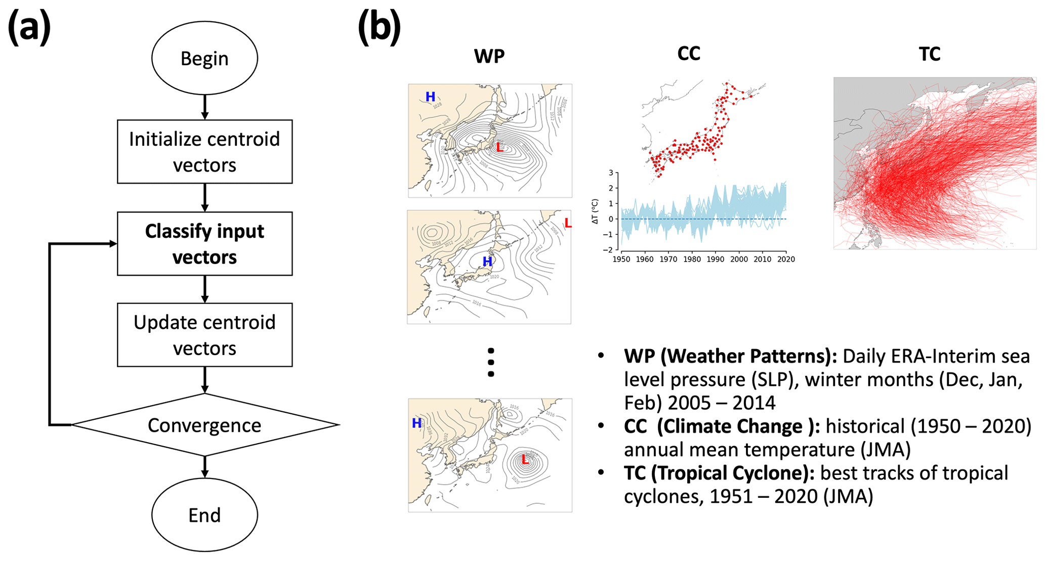
Figure 1Illustration of the k-means clustering algorithm (a) and three demonstration experiments (b). Demonstration experiments include clustering weather patterns (WPs) in terms of daily ERA-Interim sea level pressure (SLP) during winter months (December, January, and February) for 10 years (2005–2014) over the Japanese region, clustering climate change (CC) in terms of historical (1951–2020) annual-mean temperature collected from in situ weather stations in Japan, and clustering best tracks of tropical cyclones that passed the northwestern Pacific region from 1951–2020. Data were obtained from the Japan Meteorological Agency (JMA).
For a k partition, of X, and let cj denote the centroid of cluster G(j), for j ∈ K, with and a set of weight vectors . Hence, the clustering problem can be formulated as an optimization problem (Selim and Ismail, 1984), which is described by the following equation:
where wij = 1 implies that object xi belongs to cluster G(j), and d(xi, μj) denotes the distance between xi and μj for and .
The S k-means algorithm consists of four steps (Fig. 1a), which are similar to those of generic algorithms except for step (ii). The steps are described as follows.
- i.
Initialization. Initialize k centroid vectors. Although k-means has several options for initialization, we apply a randomized scheme to initialize the centroids.
- ii.
Classification. Assign an object to its most similar centroid. The S k-means algorithm uses the structural-similarity (S-SIM) (Wang et al., 2004) recognition technique to determine the most similar centroids instead of using distance measures, such as those in generic algorithms.
- iii.
Centroid calculation. Update centroid vectors by taking the mean value of the objects belonging to these clusters.
- iv.
Convergence determination. The algorithm stops when equilibrium is reached, that is, when there are no object migrations from one cluster to another. Technically, the algorithm converges if the sum of the mean square errors in centroids versus those in the previous step becomes zero in the experiments of this study. The convergence criterion is the same for all k-means variants used. A limitation of the iteration is set up to 100 to avoid the infinite loop of iterations. If equilibrium is not reached, then the process is repeated from step (ii).
S k-means is compared with E, M, and C k-means (k-means using the Euclidean distance, the Manhattan distance, and the Pearson correlation coefficient). E, M, and C k-means also follow the same procedure as indicated above except for classification scheme (ii), where the respective similarity/distance measures are used to determine the most similar centroids.
2.2 Structural similarity
The metric for the structural-similarity (S-SIM) recognition process was first introduced by Wang et al. (2004). It was developed to better predict the perceived quality of digital television and cinematic pictures. S-SIM is intended to improve the traditional peak signal-to-noise ratio or mean squared error in detecting similarities between structural signals, such as images. Intuitively, S-SIM is determined by considering the differences between two input signals (vectors x,y) across multiple aspects including “luminance”, “contrast”, and “structure”, which represent the characteristics of human visual perception. Luminance masking is a phenomenon whereby image distortions tend to be less visible in bright regions, while contrast masking is a phenomenon whereby distortions become less visible where there is significant activity or “texture” in the image. Mathematically, S-SIM is determined as follows:
where , and s(x,y) measure similarities in luminance (brightness values), contrast, and structure between sample vectors xy with weight values α, β, and γ. Let μx and μy be the mean values, σx and σy the standard deviations, and σxy the covariance of the two sample vectors x and y. Luminance, contrast, and structure similarities are then defined as , , and . Note that c1, c2 , and c3 are parameters to stabilize the division with a weak denominator. Even if , S-SIM still works quite well (Wang and Bovik, 2009); l(x,y) measures the similarity in brightness, i.e., the difference regarding mean values; c(x,y) quantifies the similarity in illumination variability, which regards standard deviations; and s(x,y) measures the correlation in spatial inter-dependencies between images and is close to the Pearson correlation coefficient. For simplification, here we set and weights and reduce the original formula to the following:
S-SIM is a symmetric index, i.e., S-SIMS-SIM(y,x). It does not satisfy the triangle inequality or non-negativity and thus is not a distance function. S-SIM ranges from −1 to 1, where −1 indicates totally dissimilar and 1 indicates totally similar. Wang and Bovik (2009) showed that S-SIM represents a powerful, easy-to-use, and easy-to-understand alternative to traditional distance metrics, such as Euclidean distance, for dealing with spatially and temporally structured data, i.e., data with strong spatial and temporal inter-dependencies. These inter-dependencies carry important information about the objects in the visual scene. S-SIM emerged as a “new-generation” similarity metric with an increasing number of applications outside the signal processing field, including hydrology and meteorology (e.g., Mo et al., 2014; Han and Szunyogh, 2018; Doan et al., 2021).
S k-means is applied to three representative clustering problems. These problems cover various types of input datasets that represent diverse issues, i.e., weather pattern (in terms of two-dimensional pressure data), historical climate change (in terms of time series), and tropical cyclone tracking data (the hybrid type of data containing both spatial and temporal information) (Fig. 1b). The details of these three tests are described below.
-
Weather pattern (WP) clustering. Group winter weather patterns in Japan. The mean sea level pressure (SLP) was obtained using ERA-Interim reanalysis data (Dee et al., 2011). The data have a horizontal resolution of 0.75∘ on a regular grid but are re-gridded to an equal-area scalable earth-type grid at a spatial resolution of 200×200 km using the nearest-neighbor interpolation method. This interpolation/regridding method is commonly applied to high-latitude domains (Gibson et al., 2017). Data collected in winter months, that is, December, January, and February (DJF), for 10 years (2005–2014) over the region from 20–50∘ N and 115–165∘ E were used. The total number of samples used is 902. Each sample has a grid size of 35 pixels ×35 pixels.
-
Climate change (CC) clustering. Group temperature-increase time series data collected over 70 years (1951–2020) from in situ weather stations run by the Japan Meteorological Agency. A simple data-quality check is implemented. Weather stations that missed (daily basis) observations for more than 10 % of the total period of interest are excluded. Therefore, 134 valid weather sites remain (see CC in Fig. 1b for the location of weather sites). The annual mean of each time series is calculated, and the climate change component is determined by subtracting the average of the first 30 years (1951–1980) from each value series.
-
Tropical cyclone (TC) tracking clustering. Group the best TC tracks from 1951 to 2020, which are retrieved from the Japan Regional Specialized Meteorological Center (RSMC) (https://www.jma.go.jp/jma/jma-eng/jma-center/rsmc-hp-pub-eg/besttrack.html, last access: 23 January 2021). Note that the RMSC provides only the best TC tracks, which have a maximum wind speed of more than 17.2 m s−1, i.e., wind force 8 on the Beaufort scale (Barua, 2019). These data contain the TC classification, maximum sustained wind speed, central pressure, and latitude and longitude of the TC centers with 6 h intervals. In this study, only TCs that passed the Japanese region, defined as the region between 25–45∘ N and 126–150∘ E, are used for the analysis. Hence, the total number of TCs feeding the k-means is 863. Because k-means clustering requires identical lengths of input vectors, the TC tracks are reconstructed so that they had an equal length of 20 segments by the method proposed by Kim et al. (2011), which has been applied in several studies (Choi et al., 2012; Kim and Seo, 2016).
As mentioned in the introduction, in addition to S k-means, the C, E, and M k-means methods that use Pearson correlation coefficients and Euclidean and Manhattan distances for the classification scheme are used for the tests. For this, we perform a total of simulations. For each simulation, 11 k settings are implemented, that is, , and for each k, 10 runs (randomized initializations) are realized. In summary, a total of runs (model realizations) are performed for the analysis.
4.1 Similarity distributions
The similarity-distribution technique developed by Doan et al. (2021) to evaluate a “global” pairwise relationship of input vectors is adopted for performance evaluation. In this study it is named the similarity distribution (S distribution, or S-D). The S distribution is a probability density function of pairwise similarities of a vector set. Let be the set of n objects; sij the pairwise similarity between two objects, which is defined as ; and F the similarity function, and . The normalized sij is defined as . By definition, sij′ ranges from 0 to 1, with the maximum value of 1 indicating perfect similarity (self-similarity) and the minimum value of 0 indicating a lack of similarity (distance to the furthest object); thus sij′ is data-dependent. As F is a symmetric function, that is, for all similarity/distance indices of interest, i.e., S-SIM, COR, ED, and MD, duplicated values are removed. Also, self-similarity values, that is, sij′ with i=j, are removed. Thus, values remained in the final set S of sij′. The S distribution, or S-D, is defined as the probability density function of the values of S. The S-Ds were then plotted together for comparison. In addition, statistical parameters, such as the mean, standard deviation, skewness, kurtosis, and Shannon entropy, were calculated to further diagnose the characteristics of the datasets of interest.
4.2 “General” silhouette analysis
As k-means clustering is an unsupervised machine learning method, it does not require “ground truth” or predefined cluster labels of an input dataset for classification. The absence of ground truth means that the algorithm can be validated only with internal validation criteria. Internal validation is to define the goodness of the clustering outcome based on the result itself to define how clustering methods optimize the homogeneity within a cluster and maximize the difference among clusters (Hassani and Seidl, 2017). There are numerous indices for clustering internal validation, though most of them are built on Cartesian geometric algebra, which is not the case with non-distance metrics like S-SIM.
Thus, this study uses the general silhouette analysis method to validate the algorithms. The general silhouette analysis is the generalized form of the silhouette analysis (Rousseeuw, 1987) that can be applicable also for non-distance metrics. This concept was first used for the evaluation of self-organizing maps by Doan et al. (2021). Silhouette analysis is a comprehensive analysis of the interpretation and validation of cluster methods. This technique offers a concise graphical representation of how well each object has been classified (Rousseeuw, 1987). The silhouette value is a measure of how coherent an object is with its cluster versus how it is separated from other clusters. Mathematically, the general silhouette coefficient (GSC) for a given object is defined as follows:
where a and b are the mean intracluster distance and mean distance to the nearest cluster, respectively. Note that the distance here is the “general” distance and not the Euclidean distance, which is originally defined in the study by Rousseeuw (1987). The general distance is the reversed normalized similarity (i.e., ) defined in Sect. 4.1, which is why here we call it the general silhouette coefficient.
The GSC values ranged from −1 to +1. A higher value indicates the goodness of the cluster assignments; that is, the object is coherent with its cluster and well separated from neighboring clusters. The clustering configuration is appropriate if most objects have high scores. In contrast, if many objects have low or negative values, then the clustering configuration performs poorly. A GSC of zero indicates that the object is on or very close to the border of two neighboring clusters, and a negative GSC indicates that the object may have been assigned the wrong cluster label.
4.3 Clustering uncertainty evaluation
Evaluating the variability or uncertainty inherent in a clustering algorithm is challenging owing to the unique nature of the clustering outcome. It is difficult to define the statistical mean, standard deviation, or range between quantiles of a given ensemble of clustering realizations.
Herein, we propose a framework for the representation/evaluation of the uncertainty in the clustering problem, which is based on a pairwise comparison of clustering realizations using a quantified index called the clustering uncertainty degree (CUD). The CUD is based on the mutual-information concept, specifically the adjusted mutual-information index. In information theory, mutual information from two random variables is used to quantify the “amount of information” obtained for one random variable by observing another random variable. The concept of mutual information is intimately linked to the entropy concept of a random variable, which is a fundamental notion in information theory that quantifies the expected “amount of information” held in this variable. In this study, mutual information is applied to evaluate the agreement between two clustering realizations (label assignments of N objects). To do so, the mathematical formula for mutual information I(UV) between two clustering realizations U and V is defined as follows:
where H(U) and H(V) are the entropies of each realization, and H(UV) is the joint entropy of the two. Entropies of clustering realizations are defined as the amount of uncertainty for partition sets of each realization.
where , and ai= |Ui| is the probability that an object pickup from U falls into class Ui at random. Similarly, for V, , where bj= |Vi| is the probability of an object from V falling into class Vj.
where is the probability that an object pickup falls into both classes Ui and Vj at random.
By definition, mutual information ranges from 0 to 1. A value of 1 indicates perfect agreement (equality) between the two clustering realizations, while values close to zero indicate that the two label assignments are largely independent. However, mutual information is weak against chance. Vinh and Epps (2009) derived the expected mutual information and proposed the concept of adjusted mutual information that can defend against chance (Vinh and Epps, 2009; Vinh et al., 2010; Romano et al., 2016). Thus, random (uniform) label assignments have an adjusted mutual-information score close to 0.0 for any number of clusters and objects (which is not the case for raw mutual information). Note that the adjusted mutual information is primarily developed to measure the “goodness” of clustering outcomes versus previously known ground truth. In this study, we diversify this primary purpose by applying the metrics to evaluate the uncertainty/consistence/convergence of clustering outcomes. Also, using the adjusted mutual information must be understood as showcased for the evaluation framework. We could also use alternative techniques, e.g., rand index, for the same purpose.
The core concept underlying the CUD, i.e., clustering uncertainty degree, is defined as follows:
By definition, CUD is a representation of pairwise dissensus of clustering realizations. The CUD ranges from 0 to 1. A value of 1 indicates the greatest dissensus or highest uncertainty between U and V, while a value of 0 indicates perfect consensus or no uncertainty. The connectivity matrix of pairwise CUDs is defined as an M × M matrix and CUD values for a pair of clustering realizations, where M is the number of clustering realizations. The connectivity matrix naturally serves as a visualization tool to assess the general uncertainty in the clustering system. Other visualization tools are also used to visualize the CUD, including a heatmap and a chord diagram (Holten, 2006). Heatmaps work like a connectivity matrix but in a more visualized form. A chord diagram is a useful graphical method for demonstrating the interrelationships between the data in a matrix. The data are plotted radially around a circle. The relationships between data points are usually drawn as arcs that connect the data.
Table 1Statistical metrics of S distributions for three demonstration input datasets, i.e., weather pattern (WP), climate change (CC), and tropical cyclone (TC). The different distance/similarity measures are structural similarity (S-SIM), the Pearson correlation coefficient (COR), Euclidean distance (ED), and Manhattan distance (MD). Statistical measures include the mean (Mean), standard deviation (SD), skewness (SKEW), kurtosis (KUR), and Shannon entropy (ENTROPY).
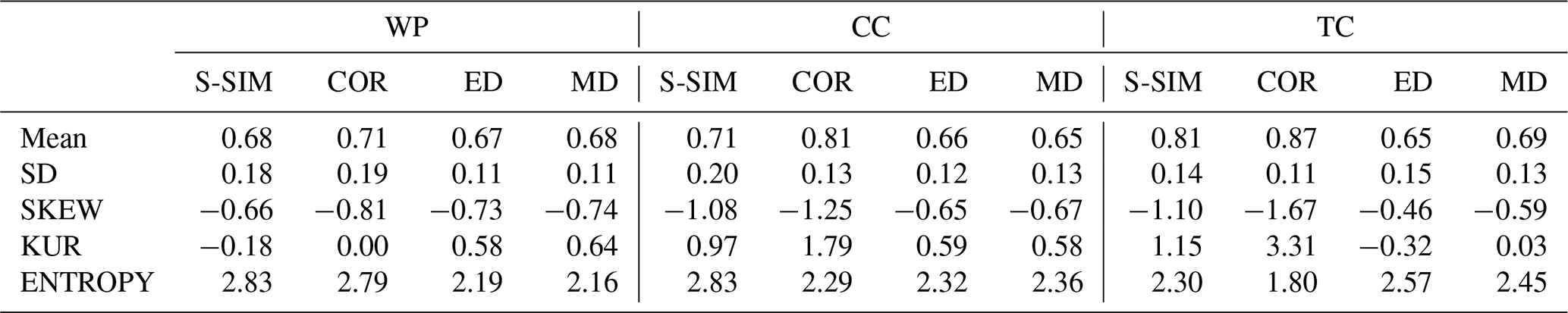
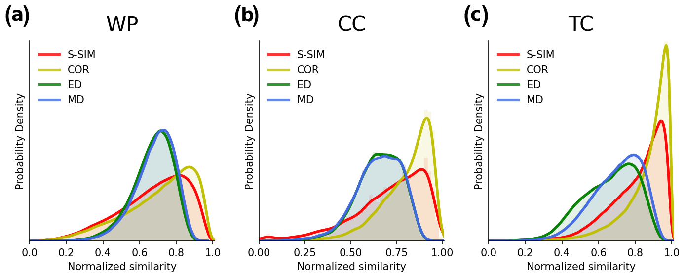
Figure 2Comparison of the S distributions of normalized pairwise similarity using the structural similarity (S-SIM), the Pearson correlation coefficient (COR), the Euclidean distance (ED), and the Manhattan distance (MD) for three demonstration experiments: WP, CC, and TC. With a population size of N, values of pairwise similarity are observed because S-SIM, COR, ED, and MD are symmetric measures, and self-similarity is excluded. Values are normalized from 0 to 1. The maximum similarity is 1, which corresponds to completely similar, and the minimum similarity is 0, which corresponds to the lowest pairwise similarity.
5.1 S distributions
Before analyzing the k-means clustering results, we diagnose the nature of the input data using S distributions (or S-Ds). S-Ds provide “global” insights into how data vectors are related to each other in four S-SIM, COR, ED, and MD topological spaces. The results, which are shown in Fig. 2, demonstrate an apparent difference in the shape of the S-Ds. Notably, the S-Ds for ED and MD appear more symmetrical than those for S-SIM and COR across the three types of input data, that is, WP, CC, and TC. For S-SIM and COR, S-Ds tend to be more tailed (both sides), with skewness over the left tail. Quantitatively, the standard deviation of S-Ds for S-SIM and COR exhibits higher values (approximately 0.13–0.20) than those for ED and MD (approximately 0.11–0.13) (Table 1), despite an exception for ED in the TC simulation. The skewness (measures the symmetry of S-Ds) exhibits negative values, meaning the distributions are left-skewed. This fact is clearly confirmed in visualized results (Fig. 2). S-SIM and COR especially exhibit higher skewness than ED and MD, particularly in the CC and TC experiments. The skew-over-left of S-SIM and COR indicates that those tend to project “hierarchical affinity” of input vectors, meaning that a given vector tends to be closer to a certain group of peers and relatively far from another group located at the opposite end of the similarity spectrum. In this sense, these results demonstrate that the discrimination ability of S-SIM and COR is higher than that of traditional distance metrics, such as ED or MD. In addition, kurtosis and Shannon entropy measure the flatness and “information value” (or “information gain” in the case of comparison) of distributions, respectively. Overall, kurtosis values are consistent with the visualized results in Fig. 2; i.e., S-Ds of S-SIM and COR tend to spread more over two tails than those of ED and MD. Entropy, on the other hand, is likely more data-dependent. It does not show obviously higher or lower trends of S-SIM and COR than those of ED and MD.
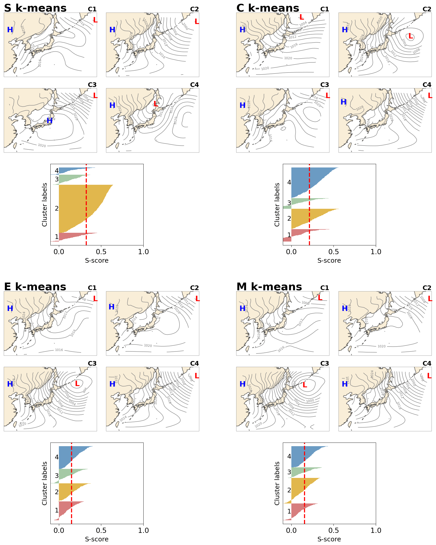
Figure 3Result for the WP experiment. The winter SLP pattern revealed by S, C, E, and M k-means with k = 4. “H” indicates the location of the high, and “L” indicates the location of the low. General silhouette analysis results are shown below the maps, where the x axis indicates the score, and the y axis presents the labels of clusters numbered 1–4. Input data are ERA-Interim SLP data, which were re-gridded to Cartesian coordinates with a resolution of 200×200 km and grid size of 35×35. Daily data for December, January, and February collected over 10 years (2005–2014) were used.
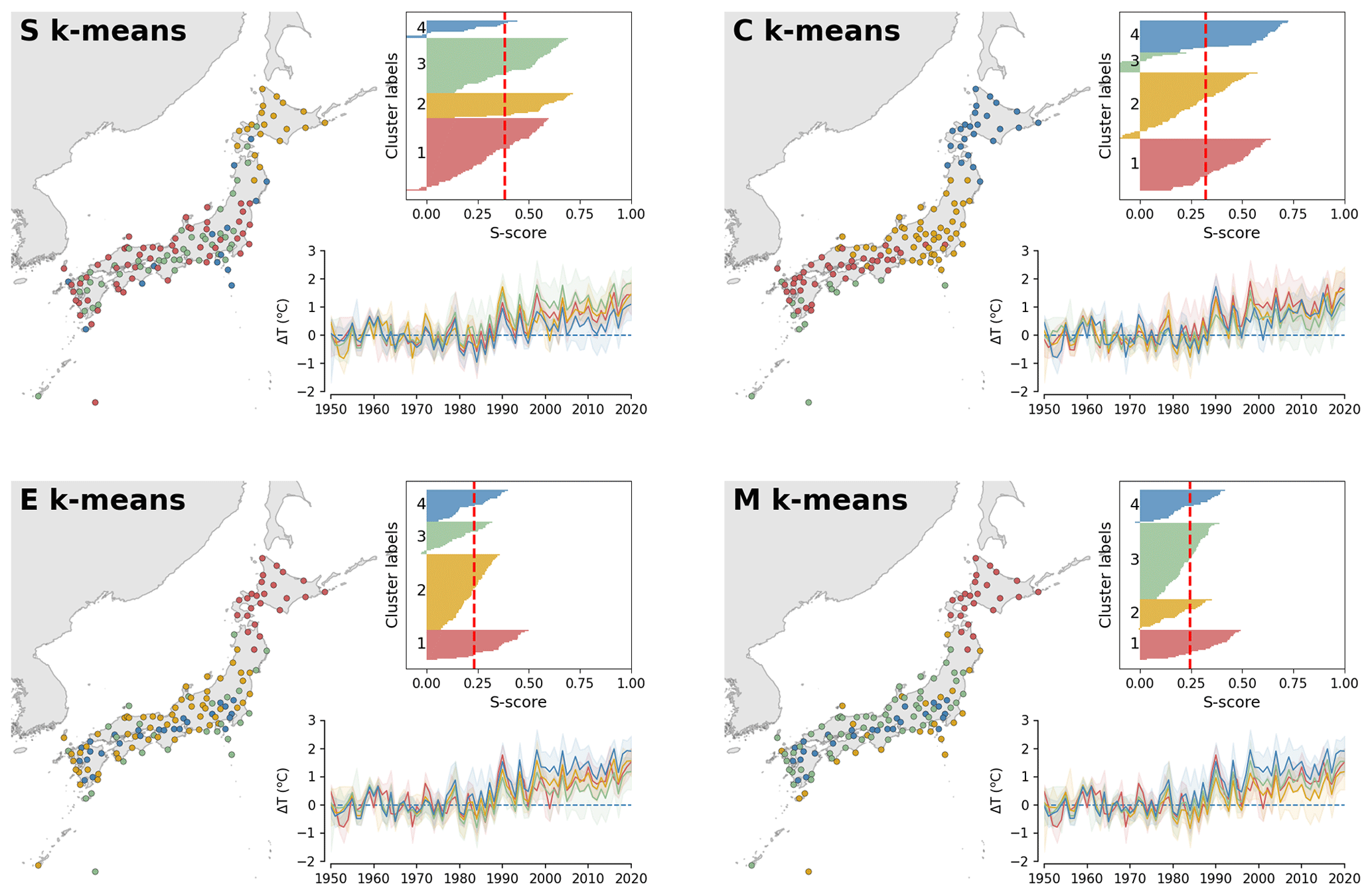
Figure 4Result for the CC experiment for clustering of climate change (temperature increase) time series over 134 weather stations over the entirety of Japan. Patterns were revealed by S, C, E, and M k-means, with k = 4. Input data correspond to annual-mean data collected over 70 years from 1951–2020 (subtracted by the mean of the first 30 years) and observed temperature achieved at in situ weather stations (dots on map) operated by the JMA. Time series of centroids and input vectors are shown in the bottom panels together with general silhouette analysis results, where the x axis indicates the score (S score), and the y axis presents the labels of clusters numbered 1–4.
5.2 Clustering results
As explained in Sect. 3, three demonstration problems, WP, CC, and TC, are conducted with different k configurations and centroid initializations, with a total of 1320 runs. Note that this study addresses the algorithm aspects (attempting to seek general insight into the system's performance regardless of problems). We do not intend to physically interpret the specific clustering outcomes, although some phenomenal explanations are provided in the article.
The clustering results are partly visualized and shown together with quantified silhouette scores in Figs. 3, 4, and 5 for WP, CC, and TC, respectively, for the configuration k = 4 and the first initialization, R0 (see the Supplement for more information). Here, we explain the k-means-detected weather patterns over the Japanese region during December, January, and February (DJF) (Fig. 3). During DJF, the weather in Japan is dominated by a winter-type pattern. The winter type is characterized by the Siberian High (develops over the Eurasian continent) and the Aleutian Low (develops over the northern North Pacific), resulting in prevailing northwesterly winds. The wind blows cold air from Siberia to Japan and causes heavy snowfall on the western coast and sunny weather on the Pacific side of the country. This winter-type pattern is clearly captured by all k-means variants, that is, C2 for S, C4 for C, C3 for E, and C4 for M k-means (Fig. 3). The silhouette analysis reveals an interesting result. S-k-means-generated cluster C2 is dominant over other clusters regarding its frequency (the thickness of each cluster label in the silhouette diagram indicates the number of members in the cluster). This result is consistent with prior knowledge of the weather patterns over the region (https://www.data.jma.go.jp/gmd/cpd/longfcst/en/tourist_japan.html, last access: 20 February 2021). Moreover, S k-means consistently shows the highest silhouette scores compared to the other algorithms for all settings (Fig. 6a), followed by C k-means. E and M k-means have lower scores than S and C k-means.
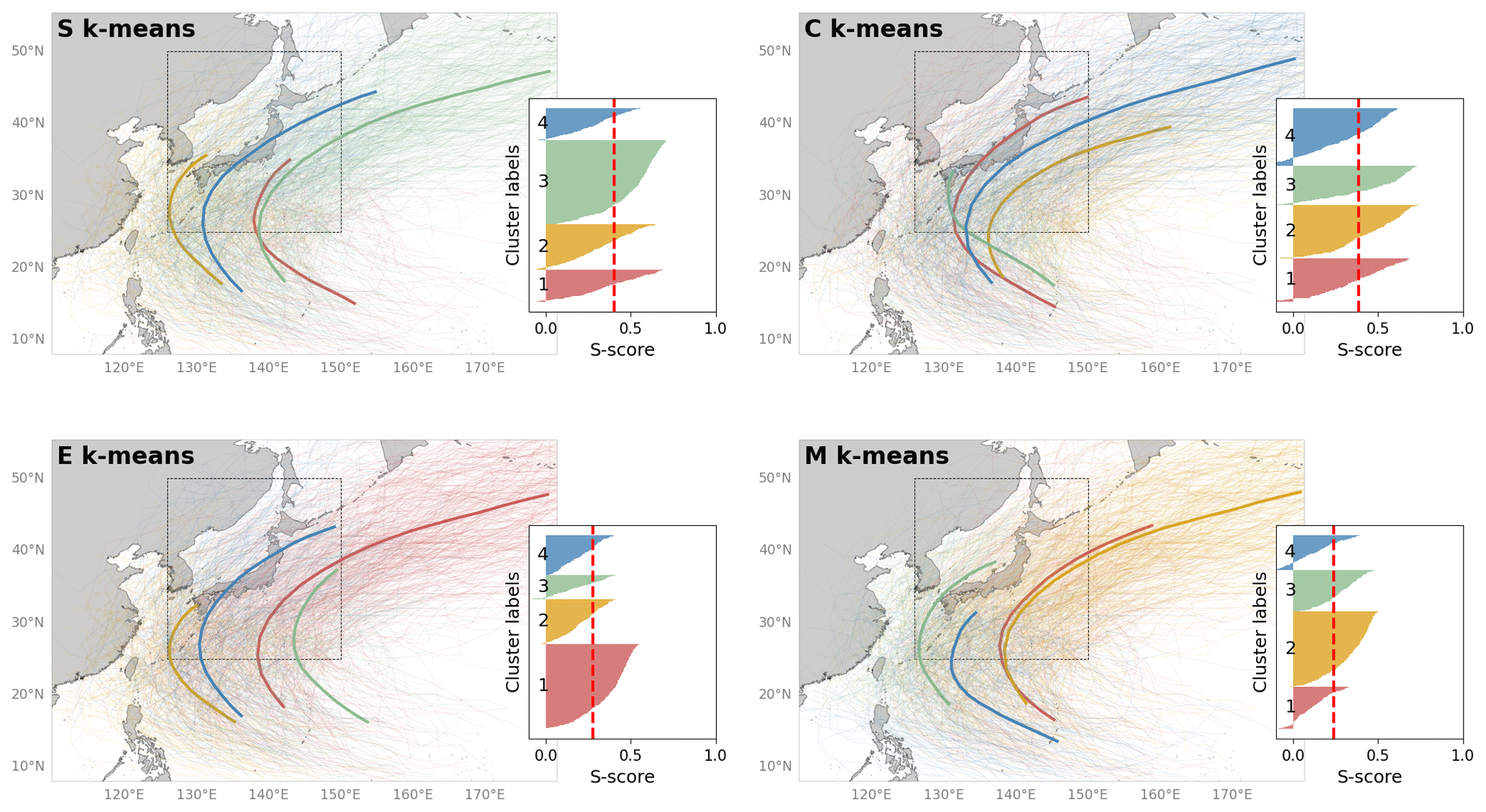
Figure 5Results of the TC experiment for clustering tropical cyclone paths. The pattern was revealed by S, C, E, and M k-means, with k = 4. Input data are the best TC tracks obtained by the JMA from 1951–2020. Only TCs that passed the dashed box in the map are used to feed the k-means. Thus, a total of 863 TC tracking data points are used. The left side of each panel shows the general silhouette analysis results, where the x axis indicates the score (S score), and the y axis presents the labels of clusters numbered 1–4. The centroid TC path is illustrated by the bold line, and the color is consistent with that in the silhouette diagram.
Regarding the CC experiment, the time series results are visualized with reference to the geographical locations of the weather stations to support interpretation (Fig. 4). Overall, the result shows that, although it is seen over all stations, the warming trend is not geographically uniform. These regional differences are well captured by the clustering. For example, the northern part (Hokkaido) is consistently separated from other regions in terms of warming rate, which is faster than the other regions. Such a result highlights the usefulness of k-means to detect regional differences, which is useful for building detailed appropriate climate change actions (though it is not the main concern of this study). Regarding clustering quality, the superiority of S and C k-means is confirmed. Like WP, S and C k-means exhibit relatively higher silhouette scores for the CC data compared with E and M k-means (Fig. 6b).
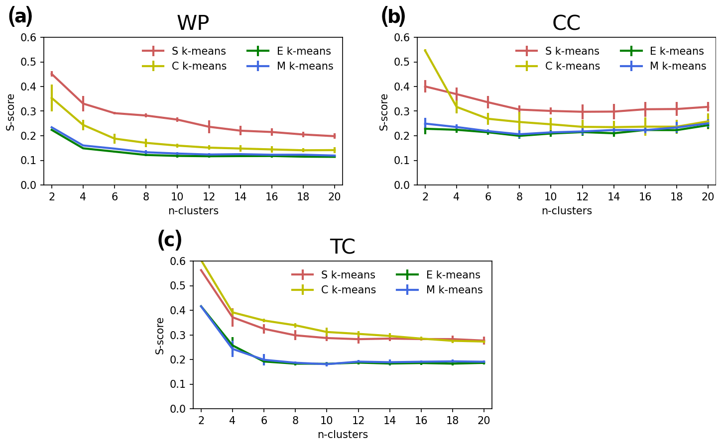
Figure 6Comparison of the average silhouette score (S score) of S, C, E, and M k-means for k=2, 4, …, 20 for three demonstration experiments: WP (a), CC (b), and TC (c). The uncertainty range in each line indicates the standard deviations of the scores among 10 runs with randomized initializations.
In addition, the TC experiment aims to determine how k-means works with hybrid spatiotemporal data. Like the above experiments, S and C k-means are likely to outperform E and M k-means, which is clearly reflected by their higher silhouette scores (Figs. 5 and 6c). Figure 5 shows the four main patterns of the TC track determined using the four clustering methods. Although there are some differences in the results among the k-means variants, such as the genesis and depression points, all determined patterns are characterized mainly by curved trajectories. These averaged patterns could be divided into two groups: (i) not crossing and (ii) crossing mainland Japan. Overall, the number of TCs in group (i) was higher than that in group (ii), with these tracks characterized by TCs containing both straight and re-curving TC trajectories forming to the east of 140∘ E (e.g., clusters 2 and 4 of S k-means in Fig. 5a). For group (ii), the averaged patterns show the TC track passing through the central area of Japan (e.g., clusters 1 and 3 of S k-means in Fig. 5a)
Consistently, the higher performance of S k-means is observed throughout the ensemble of tests, k settings, and initializations. The performance of S k-means sometimes competes with that of C k-means. The two, S and C k-means, outperform the distance-metric-based E and M k-means. It is worth noting that these results are obtained from the silhouette analysis. Additional evaluation approaches might be needed to generalize the conclusions, although this could be challenging because most objective clustering evaluations have been developed on the Cartesian geometric algebra assumption (which could work for distance metrics but might not work for non-distance measures). Therefore, it is necessary to develop new evaluation approaches beyond the distance paradigm. Another difficulty lies in the fact that, like other clustering techniques, k-means is an unsupervised machine learning technique. It works in the absence of a single ground truth to guide the classification. The absence of ground truth indicates the difficulty to define the goodness or meaningfulness of k-means clustering outcomes. Pragmatically speaking, clustering outcomes become meaningful if they are assigned a physical meaning or successfully used for practical purposes like a prediction. Doing so does not fall into the scope of this study (it is a huge work and must be addressed in an independent study); here we adopt another approach to gain insight into the behavior of the k-means variants.
By taking a careful glance at the silhouette plots shown in Fig. 3, it is possible to notice a discrepancy in S k-means compared to the rest. S k-means is likely to generate, say, “high-ordered” clustering, i.e., one dominant weather pattern (larger group size) beside several non-dominant weather patterns (smaller group size). The same trend is seen with different k settings (not shown). This agrees well with the prior knowledge recognized by the meteorological research community and local people about the winter weather patterns in Japan (explained above). This insight leads to some possible hypotheses. (i) Does S k-means perform better, i.e., closer to human perception, than other variants? (ii) Is achieving “highly ordered” clustering the intrinsic property of S k-means?
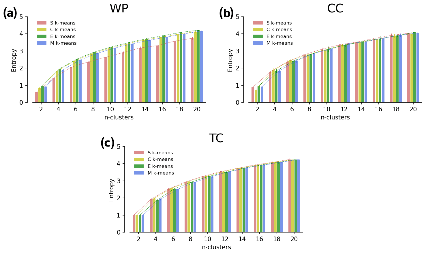
Figure 7Shannon entropy of clustering results. Comparison of the average silhouette score (S score) of S, C, E, and M k-means for k=2, 4, …, 20 for three demonstration experiments: WP (a), CC (b), and TC (c). The uncertainty range in each line indicates the standard deviations of the scores among 10 runs with randomized initializations.
To examine the hypotheses, we attempt to quantify the “orderliness” of clustering outcomes using the Shannon entropy. The results, illustrated in Fig. 7, show a good agreement between the calculated entropy values versus intuition. S k-means appears to have consistently lower entropy (highly ordered clustering) than the other algorithms for the WP experiment (Fig. 7a), but not for the CC and TC experiments (Fig. 7b, c). We can dismiss the second hypothesis (ii), which posits that achieving highly ordered clustering is an intrinsic property of S k-means because it is not universally true across all experiments. Now hypothesis (i) remains. It is possible that S k-means can achieve clustering which fits closer to human perception. However, because we do not have prior knowledge regarding the CC and TC experiments, it is too early to conclude that with complete certainty. Diversifying the clustering problems with different types of input data or for different geographical areas is necessary to obtain comprehensive insight into S k-means.
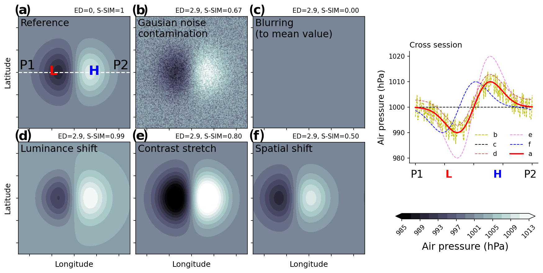
Figure 8Imagination air pressure patterns. Subpanels are the reference (a), Gaussian noise contamination (b), blurring (to mean value) (c), luminance shift (d), contrast stretch (e), and spatial shift (f). The ED (Euclidean distance) and S-SIM (structural similarity) values shown above each panel are those calculated with respect to the reference one (a). The rightmost subpanel shows the cross section (between two points P1 and P2 in a), with L and H indicating the location of imagination low and high air pressure extrema.
To further the discussion from a different aspect, we examine how the similarity between objects is recognized in k-means variants. For intuitive comprehension, we generate “imagination” weather patterns and assess the discrimination ability of similarity/distance metrics. Figure 8 illustrates the weather patterns including the reference, characterized by two extrema (low and high) symmetrically distributed over both sides (a); the Gaussian noise contamination (b); the blurring (to the mean value) (c); luminance shift (d); contrast stretch (e); and the spatial shift (f). Though the Euclidean distances from these patterns (b–e) to the reference are intentionally set to be identical (=2.9), by using S-SIM, one can rank the similarities in descending order: S-SIM(d–a) S-SIM(e–a) S-SIM(b–a) S-SIM(f–a) S-SIM(b-a) =0. This simple demonstration confirms the superiority of S-SIM in recognizing the difference between two-dimensional patterns, agreeing well with human intuition compared to ED. This implies that S-SIM could reduce the situation of random classification (i.e., an object is assigned to a centroid by chance), adding confidence to results derived from S k-means. Though this result is shown for the two-dimensional data, it is believed to be true for one-dimensional structured data like time series.
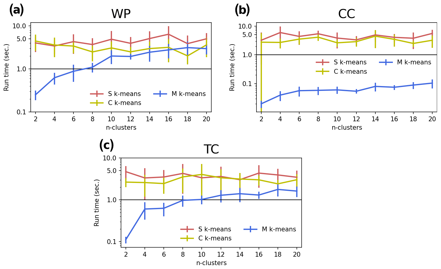
Figure 9Comparison of the run time (in seconds) of S, C, E, and M k-means for k=2, 4, … , 20 for three demonstration experiments: WP (a), CC (b), and TC (c). The uncertainty range in each line indicates the standard deviation of the scores among 10 runs with randomized initializations. Note that the y axis is logarithmically rescaled.
Computational cost is another important factor, especially in a practical sense. We measure the computational cost of each experiment and show the results in Fig. 9. Overall, S and C k-means require more time to complete the same task than E and M k-means. Roughly, S k-means required 5–6 times more computational time than E k-means. C k-means was comparable to S k-means. M k-means required less computational time than E k-means. Such a tradeoff between higher performance and computational cost should be considered when selecting an algorithm. Nevertheless, the computational cost is not a big issue, at least limited to the settings of this study; for example, the time to finish a run is less than 1 min, which is very small compared to the numerical weather prediction or climate simulation. In addition, the computational issue can be solved with the advancement of computational ability or by using a parallel computational approach.
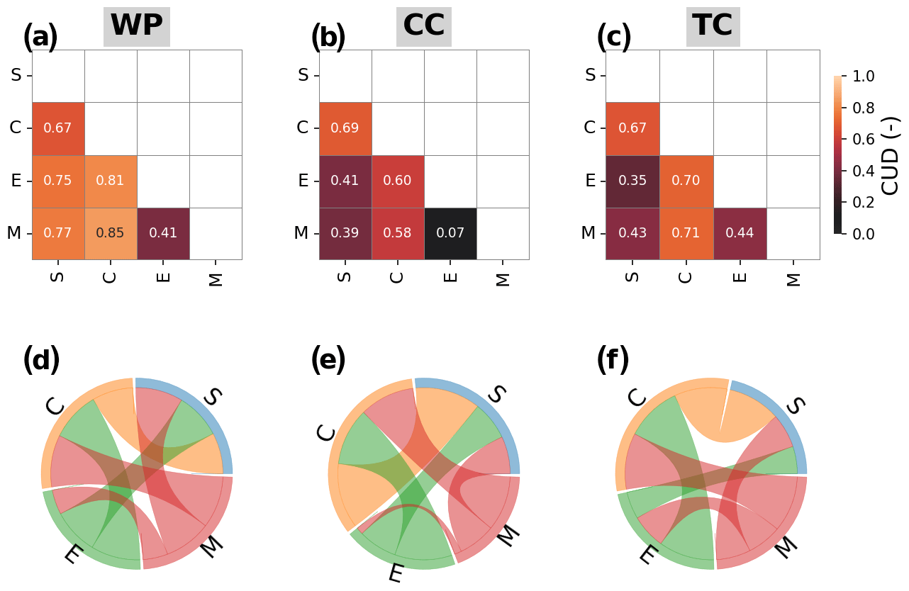
Figure 10Clustering uncertainty degree (CUD) based on adjusted mutual information (AMI) between clustering results from different k-means algorithms, i.e., S, C, E, and M k-means, for different demo experiments: WP, CC, and TC. (a, b, c) CUD in heatmaps, (d, e, f) visualization of the interconnection using the chord diagrams. Note that the results are from the configuration with k=4 and the first initialization run.
5.3 Uncertainty evaluation
The results for the clustering uncertainty evaluation framework (CUEF) are discussed here. The clustering uncertainty degree (CUD) is shown in Fig. 10 (for k=4 and run R0; the collective results are shown in Fig. 12). As explained in Sect. 4, two visualization tools, i.e., heat maps and chord diagrams, are used to visualize the clustering uncertainty. For example, Fig. 10a (WP) shows that the CUD values for S relative to C, E, and M k-means are 0.67, 0.75, and 0.77, respectively, with the heatmap. Note that the maximum CUD (=1) indicates the absolute disagreement between two clustering assignments, and the minimum CUD (=0) indicates the absolute consensus between the two. The chord diagram demonstrates the pairwise relationship in a more qualified manner. One can easily determine which algorithms (S, C, M, or E) have less consensus with another (wide arc length on the circle means less consensus), and vice versa. For example, E and M k-means show high consensus with each other. S k-means shows less uncertainty/high consensus relative to E and M compared with C k-means, particularly in the CC and TC experiments. Note that we run the four k-means variants with the randomized centroids each time. Additional runs using the same starting centroids for the four k-means variants show that the uncertainty related to the clustering algorithm selection remains regardless of whether the same or randomized staring centroids are used.
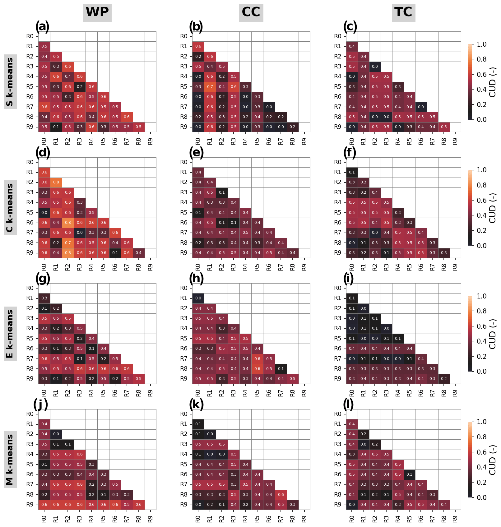
Figure 11Clustering uncertainty degree (CUD) based on adjusted mutual information (AMI) between the clustering results from different runs (10 runs indicated by R0, R1, …, R9) of different k-means algorithms, i.e., S, C, E, and M k-means (rows), for different demo experiments: WP, CC, and TC (columns). Note that the results are from the configuration with k=4 and the first initialization run.
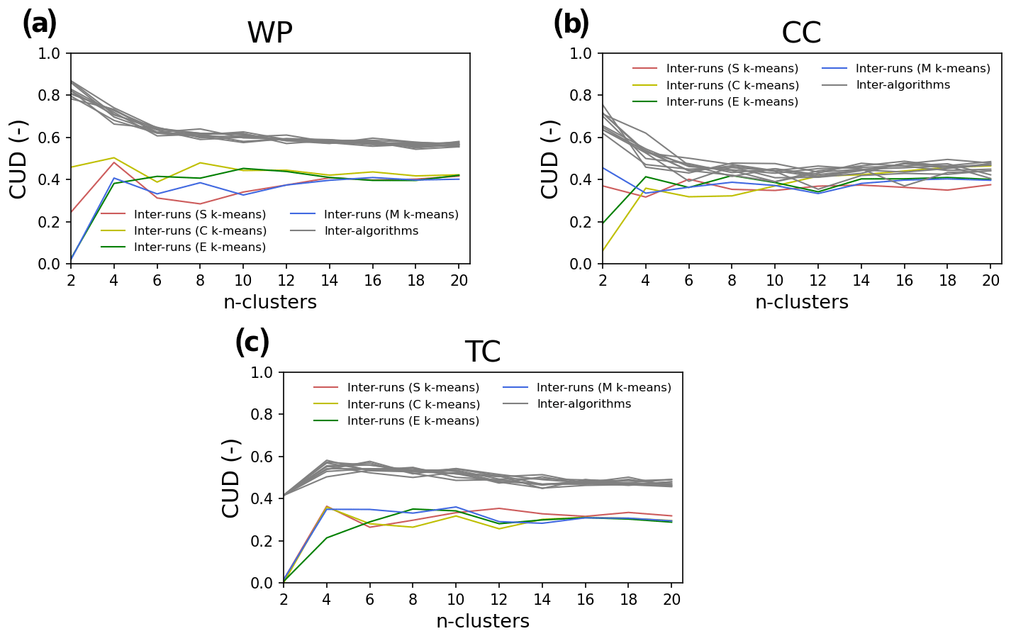
Figure 12Clustering uncertainty degree (CUD) based on adjusted mutual information (AMI) between the clustering results from different runs (10 runs indicated by R0, R1, …, R9) of different k-means algorithms, i.e., S, C, E, and M k-means (rows), for different demo experiments: WP, CC, and TC (columns). Note that the results are from the configuration .
In addition to the algorithm-wise uncertainty, we evaluate the initialization-wise uncertainty. The pairwise CUDs between runs (i.e., R0–R9 for each simulation) are shown in Fig. 11 for the WP, CC, and TC experiments with each k-means variant. The results demonstrate smaller uncertainty regarding initialization than that owing to the selection of k-means algorithms. Particularly, the initialization-wise CUDs are much lower than the algorithm-wise CUD for WP and TC. Meanwhile, in CC, the initialization-wise and algorithm-wise CUDs do not exhibit apparent differences except for k<6 (Fig. 12).
The above results demonstrate the effectiveness of CUEF (with CUD as the core concept used within the visualization framework including heatmaps or chord diagrams) in quantitatively representing/evaluating the uncertainty inherent in clustering outcomes. Heatmaps and chord diagrams are useful in offering intuitive and general comprehension of uncertainty and consensus among the outcomes. CUEF is used to evaluate algorithm-wise k-means variants in this study, but it can be used to compare clustering algorithms, e.g., affinity propagation, DBSCAN, and self-organizing maps, and initialization-wise uncertainties. Note that there are several techniques for improving the cluster initialization such as k-means (Arthur and Vassilvitskii, 2007). The result from additional simulations using k-means shows that the technique could help to reduce, though not wholly remove, the uncertainty regarding initialization.
In addition, clustering uncertainty must be understood in a broader context. It can also be induced by input data. Figures 10 and 11 show the consistently higher CUDs for WP than those for CC and TC. This means that WP yields more random clustering outcomes regardless of the algorithm used. In other words, input data themselves can possess uncertain sources for clustering. This makes sense because different data have different topologies, which can make them unsuitable or even invalid for a clustering solution. The question of whether it is valid or meaningful to apply a clustering solution to a dataset is more important than how to find the best method of clustering.
In this sense, CUEF can be used to measure the meaningfulness of clustering application to a given problem. As the big data era is coming, clustering analysis could play a vital role in discovering unseen structures of atmospheric data that are massive and inaccessible to human perception. The last decades have witnessed a wide range of clustering applications, from detecting atmospheric regimes/patterns from data (Esteban et al., 2005; Houssos et al., 2008; Spekat et al., 2010; Zeng et al., 2019; Smith et al., 2020) to using these extracted patterns for weather forecasts and climate predictions (Kannan and Ghosh, 2011; Gutiérrez et al., 2013; Le Roux et al., 2018; Pomee and Hertig, 2022) or even reconstructing historical data (Camus et al., 2014). So far, tremendous efforts have been invested in either proposing/improving clustering algorithms or inventing criteria for evaluating the goodness of the results.
A fundamental question is posed as to what the right thing to do is rather than how to do it right. In other words, it is about how to justify the choice of clustering solution rather than about looking for the way to do it right. In this sense, CUEF could help users justify the choice based directly on their data rather than rely on the experiences or literature reviews (selecting it because others are using it). This value of CUEF is significant in a time of unprecedented expansion of climate data and clustering algorithms, diversifying the needs in data mining. We recommend CUEF as a necessary procedure (or standard) for clustering techniques. Even though the final decision on whether to apply a clustering solution might depend on multiple factors, e.g., the purpose of further analysis, CUEF eventually can support the result explanation and help to make the discussion robust.
This study proposes (i) a novel k-means algorithm primarily for mining climate data and (ii) a clustering uncertainty evaluation framework. The novel k-means algorithm, called S k-means, is characterized by its ability to deal with inherent spatiotemporal structuredness in climate data. In detail, S k-means incorporates the recent innovation in signal recognition regarding structural similarity into the classification scheme, which has been primarily established based on the distance metric paradigm.
The performance of S k-means is evaluated against the other k-means variants, C, E, and M k-means, i.e., k-means using the Pearson correlation coefficient and Euclidean and Manhattan distances (C, E, and M k-means, respectively). Three demonstration tests, i.e., clustering weather patterns (spatially related data), historical climate change (time series) for long-term-recorded weather station data, and best tracks of tropical cyclones (spatiotemporal hybrid), as well as 11 k settings () for each test and for each k an ensemble of 10 randomized initializations are implemented, all resulting in a total of 1320 runs in order to obtain robust results.
The quantitative approaches, i.e., similarity distribution (S-D) and general silhouette analysis, are used to evaluate the performance of the algorithms. S-D diagrams were used to diagnose the topological relationship of input datasets in different distance/similarity spaces. The results show that structural-similarity groups are likely to have a higher ability to discriminate the data (characteristics that might be useful for clustering) than conventional distance metrics. Regarding the clustering results, the general silhouette analysis shows consistently higher scores for S and C k-means compared with E and M k-means. The superiority of S k-means clustering is followed by C k-means clustering. Both S and C k-means consistently outperform E and M k-means. The tradeoff between the clustering performance and computational resource requirement is revealed, as S k-means requires 5 to 6 times more computational time than E k-means.
S k-means could be promising as a new standard for climate data clustering/mining, which is a rising research field within the big data context. Nevertheless, certain issues must be noted when interpreting the results of this study. First, as k-means clustering is an unsupervised data mining method, it works under an assumption of no ground truth labeling information. Therefore, there is no absolute reference to define the goodness of the clustering result. In this study, the goodness of the algorithm is evaluated based on an objective calculus approach using the general silhouette analysis/score. However, this score is free from the Cartesian geometry assumption, thus allowing the algorithms to be compared with non-distance metrics; it is suggested that more evaluation and diversified clustering problems are needed to gain deeper insight into the algorithm.
Finally, another important contribution of this study is that we built a framework for clustering uncertainty evaluation for the first time, and it is primarily applicable to climate research. The evaluation framework is built on the mutual-information concept. This is the first time this concept has been adapted for clustering uncertainty evaluations in the form of the “clustering uncertainty degree” (CUD). CUD measures pairwise discrepancies among clusters, and the collective CUDs provide an overall picture of the consistency/uncertainty in the cluster algorithms. Naturally, CUD can be used to evaluate whether a given problem (input data) is preferable for clustering. In other words, if the cluster algorithm provides higher uncertainty in its outcomes, then it is not appropriate for use, and vice versa. For example, for what is shown in this study, the WP problem caused more uncertainty in clustering than the CC and TC problems. Thus, the “meaningfulness” of the clustering application for WP compared with CC and TC is questioned. We expect this clustering uncertainty evaluation framework to change the conventional agenda of data clustering by adding a procedure to evaluate its application's meaningfulness/effectiveness for given data.
The exact version of the model used to produce the results in this study and the input data and scripts used to run the model and plot all the simulations presented in this paper have been archived on GitHub (https://github.com/doan-van/S-k-means, last access: 6 July 2022) and Zenodo (https://doi.org/10.5281/zenodo.6976609; Doan, 2022).
The the input data and scripts used to run the model and plot all the simulations presented in this paper have been archived via Zenodo (https://doi.org/10.5281/zenodo.6976609; Doan, 2022).
The supplement related to this article is available online at: https://doi.org/10.5194/gmd-16-2215-2023-supplement.
QVD designed the model and developed the model code. TA, THP, TS, FC, and HK helped to design the test experiments. THP and TS helped to analyze the results. QVD prepared the manuscript with contributions from all co-authors.
The contact author has declared that none of the authors has any competing interests.
Publisher’s note: Copernicus Publications remains neutral with regard to jurisdictional claims in published maps and institutional affiliations.
This research has been partly supported by the cooperation research project between the University of Tsukuba and Nikken Sekkei Research Institute (grant no. CPI04-089).
This paper was edited by Richard Mills and reviewed by two anonymous referees.
Arthur, D. and Vassilvitskii, S.: k-means: the advantages of careful seeding, in: Proceedings of the Eighteenth Annual ACM-SIAM Symposium on Discrete Algorithms, SODA 2007, New Orleans, Louisiana, USA, 7–9 January 2007, 1027–1035, https://theory.stanford.edu/~sergei/papers/kMeansPP-soda.pdf (last access: 23 January 2023), 2007.
Barua, D. K.: Beaufort Wind Scale, in: Encyclopedia of Coastal Science, edited by: Finkl, C. W. and Makowski, C., Springer International Publishing, Cham, 315–317, https://doi.org/10.1007/978-3-319-93806-6_45, 2019.
Bradley, P. S. and Fayyad, U. M.: Refining Initial Points for K-Means Clustering, in: Proc. 15th International Conf. on Machine Learning, Morgan Kaufmann, San Francisco, CA, 91–99, 1998.
Camus, P., Menéndez, M., Méndez, F. J., Izaguirre, C., Espejo, A., Cánovas, V., Pérez, J., Rueda, A., Losada, I. J., and Medina, R.: A weather-type statistical downscaling framework for ocean wave climate, J. Geophys. Res.-Oceans, 119, 7389–7405, https://doi.org/10.1002/2014JC010141, 2014.
Chan, E. Y., Ching, W. K., Ng, M. K., and Huang, J. Z.: An optimization algorithm for clustering using weighted dissimilarity measures, Pattern Recogn., 37, 943–952, https://doi.org/10.1016/j.patcog.2003.11.003, 2004.
Choi, K.-S., Cha, Y.-M., and Kim, T.-R.: Cluster analysis of tropical cyclone tracks around Korea and its climatological properties, Nat. Hazards, 64, 1–18, https://doi.org/10.1007/s11069-012-0192-7, 2012.
Cordeiro de Amorim, R. and Mirkin, B.: Minkowski metric, feature weighting and anomalous cluster initializing in K-Means clustering, Pattern Recogn., 45, 1061–1075, https://doi.org/10.1016/j.patcog.2011.08.012, 2012.
de Amorim, R. C.: A Survey on Feature Weighting Based K-Means Algorithms, J. Classif., 33, 210–242, https://doi.org/10.1007/s00357-016-9208-4, 2016.
Dee, D. P., Uppala, S. M., Simmons, A. J., Berrisford, P., Poli, P., Kobayashi, S., Andrae, U., Balmaseda, M. A., Balsamo, G., Bauer, P., Bechtold, P., Beljaars, A. C. M., van de Berg, L., Bidlot, J., Bormann, N., Delsol, C., Dragani, R., Fuentes, M., Geer, A. J., Haimberger, L., Healy, S. B., Hersbach, H., Hólm, E. V., Isaksen, L., Kållberg, P., Köhler, M., Matricardi, M., McNally, A. P., Monge-Sanz, B. M., Morcrette, J.-J., Park, B.-K., Peubey, C., de Rosnay, P., Tavolato, C., Thépaut, J.-N., and Vitart, F.: The ERA-Interim reanalysis: configuration and performance of the data assimilation system, Q. J. Roy. Meteor. Soc., 137, 553–597, https://doi.org/10.1002/qj.828, 2011.
Doan, Q.-V.: Structural k-means algorithm (v1.0), Zenodo [code], https://doi.org/10.5281/zenodo.6976609, 2022.
Doan, Q.-V., Kusaka, H., Sato, T., and Chen, F.: S-SOM v1.0: a structural self-organizing map algorithm for weather typing, Geosci. Model Dev., 14, 2097–2111, https://doi.org/10.5194/gmd-14-2097-2021, 2021.
Eltibi, M. F. and Ashour, W. M.: Initializing k-means clustering algorithm using statistical information, Int. J. Comput. Appl., 29, 51–55, https://doi.org/10.5120/3573-4930, 2011.
Esteban, P., Jones, P. D., Martín-Vide, J., and Mases, M.: Atmospheric circulation patterns related to heavy snowfall days in Andorra, Pyrenees, Int. J. Climatol., 25, 319–329, https://doi.org/10.1002/joc.1103, 2005.
Fahim, A. M., Salem, A. M., Torkey, F. A., and Ramadan, M. A.: An efficient enhanced k-means clustering algorithm, J. Zhejiang Univ.-Sc. A, 7, 1626–1633, https://doi.org/10.1631/jzus.2006.A1626, 2006.
Forgy, E. W.: Cluster analysis of multivariate data: efficiency versus interpretability of classifications, Biometrics, 21, 768–769, 1965.
Gibson, P. B., Perkins-Kirkpatrick, S. E., Uotila, P., Pepler, A. S., and Alexander, L. V.: On the use of self-organizing maps for studying climate extremes, J. Geophys. Res.-Atmos., 122, 3891–3903, https://doi.org/10.1002/2016JD026256, 2017.
Gutiérrez, J. M., San-Martín, D., Brands, S., Manzanas, R., and Herrera, S.: Reassessing Statistical Downscaling Techniques for Their Robust Application under Climate Change Conditions, J. Climate, 26, 171–188, https://doi.org/10.1175/JCLI-D-11-00687.1, 2013.
Han, F. and Szunyogh, I.: A Technique for the Verification of Precipitation Forecasts and Its Application to a Problem of Predictability, Mon. Weather Rev., 146, 1303–1318, https://doi.org/10.1175/MWR-D-17-0040.1, 2018.
Hassani, M. and Seidl, T.: Using internal evaluation measures to validate the quality of diverse stream clustering algorithms, Vietnam J. Comput. Sci., 4, 171–183, https://doi.org/10.1007/s40595-016-0086-9, 2017.
Holten, D.: Hierarchical Edge Bundles: Visualization of Adjacency Relations in Hierarchical Data, IEEE T. Vis. Comput. Gr., 12, 741–748, https://doi.org/10.1109/TVCG.2006.147, 2006.
Houssos, E. E., Lolis, C. J., and Bartzokas, A.: Atmospheric circulation patterns associated with extreme precipitation amounts in Greece, Adv. Geosci., 17, 5–11, https://doi.org/10.5194/adgeo-17-5-2008, 2008.
Huang, J. Z., Ng, M. K., Rong, H., and Li, Z.: Automated variable weighting in k-means type clustering, IEEE T. Pattern Anal., 27, 657–668, https://doi.org/10.1109/TPAMI.2005.95, 2005.
Jancey, R. C.: Multidimensional group analysis, Aust. J. Bot., 14, 127–130, 1966.
Kannan, S. and Ghosh, S.: Prediction of daily rainfall state in a river basin using statistical downscaling from GCM output, Stoch. Env. Res. Risk A., 25, 457–474, https://doi.org/10.1007/s00477-010-0415-y, 2011.
Kantardzic, M.: Data mining: concepts, models, methods, and algorithms, John Wiley & Sons, https://www.wiley.com/ense/Data+Mining:+Concepts,+Models,+Methods,+and+Algorithms,+3rd+Edition-p-9781119516040 (last access: 20 February 2023), 2011.
Katsavounidis, I., Jay Kuo, C.-C., and Zhang, Z.: A new initialization technique for generalized Lloyd iteration, IEEE Signal Proc. Lett., 1, 144–146, https://doi.org/10.1109/97.329844, 1994.
Khan, S. S. and Ahmad, A.: Cluster center initialization algorithm for K-means clustering, Pattern Recogn. Lett., 25, 1293–1302, https://doi.org/10.1016/j.patrec.2004.04.007, 2004.
Kim, H.-K. and Seo, K.-H.: Cluster Analysis of Tropical Cyclone Tracks over the Western North Pacific Using a Self-Organizing Map, J. Climate, 29, 3731–3751, https://doi.org/10.1175/JCLI-D-15-0380.1, 2016.
Kim, H.-S., Kim, J.-H., Ho, C.-H., and Chu, P.-S.: Pattern Classification of Typhoon Tracks Using the Fuzzy c-Means Clustering Method, J. Climate, 24, 488–508, https://doi.org/10.1175/2010JCLI3751.1, 2011.
Lai, J. Z. C. and Huang, T.-J.: Fast global k-means clustering using cluster membership and inequality, Pattern Recogn., 43, 1954–1963, https://doi.org/10.1016/j.patcog.2009.11.021, 2010.
Le Roux, R., Katurji, M., Zawar-Reza, P., Quénol, H., and Sturman, A.: Comparison of statistical and dynamical downscaling results from the WRF model, Environ. Model. Softw., 100, 67–73, https://doi.org/10.1016/j.envsoft.2017.11.002, 2018.
Lloyd, S. P.: Least square quantization in PCM. Bell Telephone Laboratories Paper, Lloyd, SP: Least squares quantization in PCM, IEEE Trans Inf. Theor19571982, 18, 11, 1957.
MacQueen, J.: Some methods for classification and analysis of multivariate observations, in: Proceedings of the fifth Berkeley symposium on mathematical statistics and probability, University of California Press, 281–297, 1967.
Mo, R., Ye, C., and Whitfield, P. H.: Application potential of four nontraditional similarity metrics in hydrometeorology, J. Hydrometeorol., 15, 1862–1880, 2014.
Overpeck, J. T., Meehl, G. A., Bony, S., and Easterling, D. R.: Climate Data Challenges in the 21st Century, Science, 331, 700–702, https://doi.org/10.1126/science.1197869, 2011.
Pelleg, D. and Moore, A. W.: X-means: Extending K-means with Efficient Estimation of the Number of Clusters, in: Proceedings of the Seventeenth International Conference on Machine Learning (ICML '00), Morgan Kaufmann Publishers Inc., San Francisco, CA, USA, 727–734, https://www.cs.cmu.edu/~dpelleg/download/xmeans.pdf (last access: 6 July 2022), 2000.
Perez, J., Mexicano, A., Santaolaya, R., Hidalgo, M., Moreno, A., and Pazos, R.: Improvement to the K-Means algorithm through a heuristics based on a bee honeycomb structure, in: 2012 Fourth World Congress on Nature and Biologically Inspired Computing (NaBIC), 2012 Fourth World Congress on Nature and Biologically Inspired Computing (NaBIC), Mexico City, Mexico, 5–9 November 2012, 175–180, https://doi.org/10.1109/NaBIC.2012.6402258, 2012.
Pérez-Ortega, J., Almanza-Ortega, N. N., Vega-Villalobos, A., Pazos-Rangel, R., Zavala-Díaz, C., and Martínez-Rebollar, A.: The K-means algorithm evolution, in: Introduction to Data Science and Machine Learning, IntechOpen, https://doi.org/10.5772/intechopen.85447, 2019.
Pomee, M. S. and Hertig, E.: Precipitation projections over the Indus River Basin of Pakistan for the 21st century using a statistical downscaling framework, Int. J. Climatol., 42, 289–314, https://doi.org/10.1002/joc.7244, 2022.
Romano, S., Vinh, N. X., Bailey, J., and Verspoor, K.: Adjusting for chance clustering comparison measures, J. Mach. Learn. Res., 17, 4635–4666, 2016.
Rousseeuw, P. J.: Silhouettes: a graphical aid to the interpretation and validation of cluster analysis, J. Comput. Appl. Math., 20, 53–65, 1987.
Selim, S. Z. and Ismail, M. A.: K-Means-Type Algorithms: A Generalized Convergence Theorem and Characterization of Local Optimality, IEEE T. Pattern Anal., PAMI-6, 81–87, https://doi.org/10.1109/TPAMI.1984.4767478, 1984.
Smith, E. T., Lee, C. C., Barnes, B. B., Adams, R. E., Pirhalla, D. E., Ransibrahmanakul, V., Hu, C., and Sheridan, S. C.: A Synoptic Climatological Analysis of the Atmospheric Drivers of Water Clarity Variability in the Great Lakes, J. Appl. Meteorol. Clim., 59, 915–935, https://doi.org/10.1175/JAMC-D-19-0156.1, 2020.
Spekat, A., Kreienkamp, F., and Enke, W.: An impact-oriented classification method for atmospheric patterns, Phys. Chem. Earth, 35, 352–359, https://doi.org/10.1016/j.pce.2010.03.042, 2010.
Su, T. and Dy, J. G.: In search of deterministic methods for initializing K-means and Gaussian mixture clustering, Intell. Data Anal., 11, 319–338, https://doi.org/10.3233/IDA-2007-11402, 2007.
Sydow, A.: Tou, JT/Gonzalez, RC, Pattern Recognition Principles, London-Amsterdam-Dom Mills, Ontario-Sydney-Tokyo, Addison-Wesley Publishing Company, Z. Angew. Math. Mech., 57, 353–354, 1977.
Vinh, N. X. and Epps, J.: A novel approach for automatic number of clusters detection in microarray data based on consensus clustering, in: 2009 Ninth IEEE International Conference on Bioinformatics and BioEngineering, Taichung, Taiwan, 22–24 June 2009, 84–91, https://doi.org/10.1109/BIBE.2009.19, 2009.
Vinh, N. X., Epps, J., and Bailey, J.: Information theoretic measures for clusterings comparison: Variants, properties, normalization and correction for chance, J. Mach. Learn. Res., 11, 2837–2854, 2010.
Wang, Z. and Bovik, A. C.: Mean squared error: Love it or leave it? A new look at signal fidelity measures, IEEE Signal Proc. Mag., 26, 98–117, 2009.
Wang, Z., Bovik, A. C., Sheikh, H. R., and Simoncelli, E. P.: Image quality assessment: from error visibility to structural similarity, IEEE T. Image Process., 13, 600–612, 2004.
Wu, X., Kumar, V., Ross Quinlan, J., Ghosh, J., Yang, Q., Motoda, H., McLachlan, G. J., Ng, A., Liu, B., Yu, P. S., Zhou, Z.-H., Steinbach, M., Hand, D. J., and Steinberg, D.: Top 10 algorithms in data mining, Knowl. Inf. Syst., 14, 1–37, https://doi.org/10.1007/s10115-007-0114-2, 2008.
Zeng, S., Vaughan, M., Liu, Z., Trepte, C., Kar, J., Omar, A., Winker, D., Lucker, P., Hu, Y., Getzewich, B., and Avery, M.: Application of high-dimensional fuzzy k-means cluster analysis to CALIOP/CALIPSO version 4.1 cloud–aerosol discrimination, Atmos. Meas. Tech., 12, 2261–2285, https://doi.org/10.5194/amt-12-2261-2019, 2019.