the Creative Commons Attribution 4.0 License.
the Creative Commons Attribution 4.0 License.
 | 20 Apr 2023
Forecasting tropical cyclone tracks in the northwestern Pacific based on a deep-learning model
Liang Wang
Bingcheng Wan
Shaohui Zhou
Haofei Sun
Zhiqiu Gao
Tropical cyclones (TCs) are one of the most severe meteorological disasters, making rapid and accurate track forecasts crucial for disaster prevention and mitigation. Because TC tracks are affected by various factors (the steering flow, the thermal structure of the underlying surface, and the atmospheric circulation), their trajectories present highly complex nonlinear behavior. Deep learning has many advantages in simulating nonlinear systems. In this paper, based on deep-learning technology, we explore the movement of TCs in the northwestern Pacific from 1979 to 2021, divided into training (1979–2014), validation (2015–2018), and test sets (2019–2021), and we create 6–72 h TC track forecasts. Only historical trajectory data are used as input for evaluating the forecasts of the following three recurrent neural networks utilized: recurrent neural network (RNN), long short-term memory (LSTM), and gated recurrent unit (GRU) models. The GRU approach performed best; to further improve forecast accuracy, a model combining GRU and a convolutional neural network (CNN) called GRU_CNN is proposed to capture the characteristics that vary with time. By adding reanalysis data of the steering flow, sea surface temperatures, and geopotential height around the cyclone, we can extract sufficient information on the historical trajectory features and three-dimensional spatial features. The results show that GRU_CNN outperforms other deep-learning models without CNN layers. Furthermore, by analyzing three additional environmental factors through control experiments, it can be concluded that the historical steering flow of TCs plays a key role, especially for short-term predictions within 24 h, while sea surface temperatures and geopotential height can gradually improve the 24–72 h forecast. The average distance errors at 6 and 12 h are 17.22 and 43.90 km, respectively. Compared with the 6 and 12 h forecast results (27.57 and 59.09 km) of the Central Meteorological Observatory, the model proposed herein is suitable for short-term forecasting of TC tracks.
- Article
(2912 KB) - Full-text XML
-
Supplement
(5389 KB) - BibTeX
- EndNote


The northwestern Pacific is the most active basin for tropical cyclones (TCs) in the world, generating over one-third of the total number of TCs (Gray, 1968). China, located on the western side of the Pacific Ocean, with a coastline longer than 18 000 km, is one of the countries most severely influenced by TCs. These storm systems are accompanied by strong winds, heavy precipitation, and storm surges, resulting in severe disasters that affect human lives and economic growth (Goldenberg et al., 2001). Studies have shown that global warming will progressively intensify TCs over time (Emanuel, 2017; Schulthess et al., 2019). Since disasters caused by TCs are unavoidable and potentially destructive, accurately predicting the movement of TCs can provide sufficient preparation time for people in affected areas to implement disaster mitigation strategies.
Given the uncertainty of TC movements, the complexity and nonlinearity inherent in the atmospheric system, and the scarcity of ocean-based observational data, accurately predicting the center positions and intensities of TCs is a challenge. Currently, forecasting methods for TCs are mainly divided into two categories, with the primary method being numerical weather prediction (NWP). NWP calculates the approximate solution of partial differential equations involving atmospheric state variables when the initial conditions and boundary conditions of the atmosphere are known. In this way, some elements, such as the tracks and intensities of the TCs, can be solved iteratively; GRAPES-TYM (CMA), GFS (NCEP), and IFS (ECWMF) are the main NWP models. Although these model forecasts can provide accurate results, there are limitations in methods relying on high-performance computers and requiring precise initial conditions. At the same time, ensemble forecast methods (GRAPES-GEFS, ECMWF-EPS, NCEP-GEFS) have been used to reduce the influence of various uncertainties on the numerical prediction results (Goerss, 2000). The other forecasting method is a statistical model, which generally utilizes multiple regression. The statistical model is mainly based on the relationship between the movement of the TC and its specific historical characteristics, but it usually does not consider any physical processes. The National Hurricane Center has successively adopted statistical models such as NHC64 (taking observational data and historical 12 h movements as factors), NHC67 (increasing factors based on NHC64), CLIPER (climate persistence factors; Neumann and Hope, 1972), and NHC72 (a combination of NHC67 and CLIPER). Most traditional TC statistical models adopt a linear regression model, and it is difficult for this approach to address the nonlinear problems in TC track forecasting (Roy and Kovordányi, 2012). At the same time, manual feature selection is unable to produce accurate predictions. CLP5 had the largest mean absolute error (MAE) of all models for TCs occurring from the eastern Pacific and North Atlantic (Boussioux et al., 2022). Li-Min et al. (2009) used the back propagation (BP) neural network to predict that the average distance error of the 6 h movement track of six typhoons in 2005 improved by 36.9 km, compared with CLIPER.
Deep learning is an emerging application of supercomputing that is continuously being developed; many researchers have tried to adopt this technology to forecast weather and meteorological elements, including visibility (Ortega et al., 2022), wind speeds (Liu et al., 2018), radar echoes (Klein et al., 2015), and precipitation nowcasting (Shi et al., 2015). Deep learning is a statistical model that solves nonlinear and complex relationships from historical sample data based on neural network algorithms. The weight factor between network nodes is automatically adjusted through repeated training; thus, neural network algorithms have the advantages of strong adaptability and fault tolerance. TCs have complex dynamic mechanisms and are easily affected by many factors, including environmental steering flow, beta effects, underlying surface conditions, the asymmetric structure of the inner core, and mesoscale circulations (Chan and Kepert, 2010). Artificial neural networks (ANNs) have been applied to predict TC tracks due to their strong learning ability and advantages in simulating nonlinear systems. Until the 2010s, ANN and BP networks were the mainstream neural network methods for forecasting TC tracks (Ali et al., 2007; Li-Min et al., 2009; Wang et al., 2011). Since the mid-2010s, more new methods have been introduced into TC prediction due to the development of deep-learning technology. Recurrent neural networks (RNNs) are suitable for TC track forecasting owing to their ability to handle time series data of arbitrary lengths. Moradi Kordmahalleh et al. (2015) applied a sparse RNN to Atlantic hurricane trajectory prediction using the dynamic time-warping (DTW) method to measure the hurricane most similar to the target hurricane for training. Gao et al. (2018) used long short-term memory (LSTM) to predict typhoon tracks in the northwestern Pacific Ocean; the ratio of the cyclone training set and test set was set at 8:2, and the 24 h prediction error could reach 105 km. Alemany et al. (2018) proposed an RNN based on a grid system to predict hurricanes in the Atlantic, potentially improving the 6 h prediction accuracy with a root mean square error (RMSE) of 0.11 for the test set. Kim et al. (2018) performed a TC identification task based on ConvLSTM to train WRF-simulated data, and the results show that the average precision of the forecast was improved by 78.99 % compared to those of a convolutional neural network (CNN). These CNNs have attracted attention given their suitability for processing 2D image data; they maintain spatial correlations by implementing convolution layers and then pooling layers for feature extraction. Giffard-Roisin et al. (2020) combined historical trajectory data with wind field reanalysis data as input to a CNN and predicted Atlantic hurricane tracks since 1979, with an average error of 32.9 km for 6 h predictions.
Making full use of different types of data is essential for deep learning. TC-related data are mainly divided into the following three categories: observational trajectory data, remote sensing data, and meteorological reanalysis field data. A multi-modal approach enables more accurate predictions than an approach using a single data source does. Zhang et al. (2018) developed a matrix neural network (MNN) model that preserves the spatial information of the TC tracks, and it has demonstrated the ability to provide more accurate results compared with other models (GRU, LSTM, multi-layer perceptron, and RNN). Ruttgers et al. (2019) built generation adversarial networks (GANs), adding satellite images to predict the coordinates of the typhoon center and to generate cloud maps of future typhoons. Liu et al. (2022) proposed a new deep-learning-based model, DBFNet, to effectively fuse the inherent features of cyclones and to reanalyze 2D pressure field data. The above studies have shown that deep-learning models that incorporate multiple data types can improve the track forecast of TCs to a certain extent. Still, most of them have neglected to describe and analyze the meteorological factors that affect the movement of TCs, ignoring valuable features. The 6 h average distance error between the predicted and real location by the fusion network (wind+track) is 32.9 km, while the network prediction results without adding wind variables are 35 km (Giffard-Roisin et al., 2018), which indicates that the addition of meteorological field variables can effectively improve the prediction accuracy.
This paper attempts to propose a new method for TC track prediction based on a combination of CNN and GRU models that incorporate data regarding the trajectory, steering airflow, sea surface temperatures, and geopotential height as input features, aiming to improve the accuracy of TC track forecasts by leveraging big data. The main contents of this paper are as follows. Section 2 introduces the necessary data and data preprocessing. Section 3 describes the experimental design and the framework of the fusion model (GRU_CNN) proposed in this paper. Section 4 presents the experimental results and comparative analysis, and Sect. 5 provides a summary and discussion of shortcomings and directions for future work.
2.1 Data
The data used in this paper are trajectory data and reanalysis environmental data. The TC track data come from the International Best Track Archive for Climate Stewardship (IBTrACS), which encompasses all TCs globally. For each TC, the latitude, longitude, central pressure, maximum wind speed, direction, moving speed, and other data are recorded at 3 h intervals. The IBTrACS dataset contains data from different basins where cyclones show different characteristics; thus, this paper only selects TCs that occur in the northwestern Pacific Ocean. To better mine the hidden information, 19 movement characteristics were obtained, including the past 24 h longitude; latitude; central atmospheric pressure; maximum wind speed; meridional moving speed; zonal moving speed; moving direction and speed; the difference between those values and those at the current time; and the angle, zonal distance, and meridional distance formed between the data over the past 24 h and in the present moment. Because they are influenced by the earth's rotation, TCs will be biased to the northwest (Kitade, 1981). The Coriolis parameters corresponding to the latitude of the TCs in the past 24 h are also included.
Both observational and theoretical studies have shown that TC movement is closely related to large-scale airflow fields (Holland, 1983), and TC movement is mainly affected by the steering flow (Brand et al., 1981; Chan, 1984). Interactions among weather systems, the subtropical anticyclone, westerlies, and the Tibetan High will also affect the movement of cyclones (George and Gray, 1976; Chan et al., 1980). The geopotential heights of 300, 500, and 700 hpa are selected as the locations for the high-, middle-, and low-level circulation data, respectively. In addition, the underlying surface conditions must be considered, and, in the case of a weak guidance environment, TCs tend to move towards warmer sea surface temperatures (Sun et al., 2017; Katsube and Inatsu, 2016). Meteorological environmental data are obtained by downloading high-resolution ERA5 reanalysis data from the European Centre for Medium-Range Forecasting (ECMWF). Holland (1984) noted that the deep mean circulation from 850 to 300 hpa can better represent the direction of a TC. Therefore, the environmental data for the preceding 24 h were extracted as follows:
-
For the u and v component data of the wind field on the four isobaric surfaces (300, 500, 700, 850 hpa), we centered the TC and extended 10∘ outward in the zonal and meridional directions, respectively. Since the resolution of the selected reanalysis data is , a 21×21 grid can be formed.
-
For the sea surface temperature (SST), we once again extended 10∘ outward in the zonal and meridional directions from the TC center to form a 21×21 grid.
-
For the geopotential heights of 300, 500, and 700 hpa, we extended a grid +35∘ to the north, −10∘ to the south, −40∘ to the west, and +40∘ to the east from the center of the TC, forming a 46×81 grid.
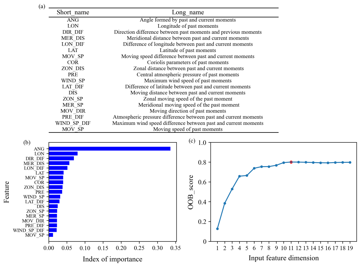
Figure 1(a) Table displaying the short and long names of features, (b) the importance index of features, and (c) the OOB_score of different feature combinations based on the random forest (red dot indicates the maximum value).
2.2 Data preprocessing
2.2.1 Devortexing
Because the actual weather circulation is very complex and includes information about the TC itself, the surrounding airflow, and the interaction between the two, it is necessary to separate the cyclone vortex from the surrounding airflow to obtain the steering flow. The most commonly used method (Lownam, 2001; Galarneau and Davis, 2013) corrects the vorticity and divergence by solving the change in the velocity stream and potential functions, respectively, and then calculates the modified velocity field. The modified flow field can be interpreted as having a non-rotating wind and a non-diverging wind. There must be potential velocity in the irrotational motion and a stream function in the non-divergent motion. The relationship between them can be expressed as follows:
where ψ is the stream function without divergence, ζ is the relative vorticity, and νΨ is the non-divergent wind (rotating wind). To define the rotating wind, the vorticity outside the vortex radius is set to zero, and ψ=0 is specified on the horizontal boundary. The iterative relaxation method is used to solve the stream function of Eq. (1) at all layers and then to calculate νΨ using Eq. (2). In the case of divergence, Eqs. (1) and (2) are replaced by the following:
where χ is the potential velocity, δ is the divergence, and νχ is the non-vorticity wind. The divergence outside the vortex radius is set to zero, and the potential function χ=0 on the boundary of the region. The velocity potential can be solved in the same manner to calculate νχ. The ambient wind field with the vortex removed can be obtained by subtracting the rotating wind and divergent wind from the original wind field, V, as follows:
2.2.2 Random forest
By sorting features based on importance, random forest selects the best feature combination and reduces the input feature dimensions that efficiently direct variables for machine learning models (Díaz-Uriarte and Alvarez De Andrés, 2006; Genuer et al., 2010). The random forest contains N decision trees, and N is generally set to 100. Since bootstrapping (random sampling with replacement) is used to generate the random decision tree, all samples are not in the generation process of a tree, and the unused samples are called out-of-bag (OOB) samples. Through OOB samples, the accuracy of this tree can be evaluated.
Before model training, it is necessary to determine whether the 19 trajectory features all have an impact on the prediction results. Figure 1a shows the long name corresponding to the short name of 19 input features, and Fig. 1b shows the 19 features' order of importance, calculated using the random forest method. For forecasting the difference in longitude and latitude within the following 72 h, characteristics like the historic longitude or the angle formed by the historical moment and the current moment are significant. The decision about whether to exclude some less-important features, however, requires further consideration. The OOB scores under different input feature dimensions are computed, with variables input in the order of importance, as shown in Fig. 1c. In the case in which the first 11 features are sorted by importance, the OOB score is the highest, and the features added later will no longer affect the result; in other words, the best combination is that of the first 11 features.
3.1 Experimental design
Our goal is to predict the TC movements for the following 6–72 h using the trajectory data and the surrounding environmental field from the previous 24 h. We explore TC movement in the northwestern Pacific from 1979 to 2021 and consider the longitudinal and latitudinal changes in the following 6–72 h as the quantitative prediction variables, with the center of the TC at the current time being the reference point. Since the maximum forecast hour is 72 and the input sequence time length is 24 h, TCs that persist for longer than 96 h are removed. All samples obtained based on the sliding window of the input–prediction sequence length are divided into the following three groups in chronological order: training set (1979–2014), validation set (2015–2018), and test set (2019–2021). There are 36 473 samples, of which 90 % are trained, and the remaining 10 % are validated; 49 TCs from 2019 to 2021 are used for testing, and the number of test samples is 2095.
3.2 Model framework
3.2.1 Recurrent neural network
RNNs can process sequences of any length using neurons with self-feedback, characterized by architectural features intentionally designed to preserve historical information, showing a remarkable ability to process sequential data (Graves et al., 2013; Bathla, 2020; Wang and Fu, 2020). However, simple RNNs have difficulty dealing with the long-term dependence of the sequence; when the sequence length exceeds a certain threshold, the information may disappear during the transmission process, resulting in large deviations in prediction accuracy. The LSTM network proposed by Hochreiter and Schmidhuber (1997) can avoid the gradient disappearance and explosion phenomena that occur in the standard RNN. While GRU (Cho et al., 2014) is an improved and optimized neural network based on LSTM, it has a faster convergence speed and maintains accuracy levels close to those of LSTM.
3.2.2 Convolutional neural network
CNNs can extract features automatically by processing the input patterns and translating the same convolution kernel from top to bottom and from left to right. The spatial relationship is fixed with the distribution of neurons, and the local connection and weight sharing of neurons reduce the training complexity by reducing the number of parameters. Lecun et al. (1998) first used CNN for handwritten-character recognition with average pooling and the tanh activation function. Krizhevsky et al. (2012) proposed the AlexNet model in the ImageNet competition, using the ReLU function instead of the traditional tanh function to introduce nonlinearity and to solve the gradient disappearance problem of the activation function when the network was relatively deep, employing maximum pooling to avoid the blurring effect of average pooling. Ioffe and Szegedy (2015) applied batch normalization to image classification models, which significantly accelerated the training of deep networks, and batch normalization helped alleviate the problem of gradients exploding or vanishing.
3.2.3 GRU_CNN
Due to differences in the data sources, a new model must be developed to integrate the four information sources into the neural network using the Keras deep-learning framework. The specific model structure is shown in Fig. 2. The 3D meteorological data are superimposed on the geopotential height (pressure level), so the input data for the CNN consist of multiple three-dimensional matrices; that is, the area of the light-gray shaded region in Fig. 2 represents 3D tensor input layers of the CNN model. The solid gray arrow represents the TimeDistributed layer that is applied to a series of tensors in the processing of the time dimension. In addition, the CNN adopts a typical architecture with alternating convolution layers (Conv layers) and maximum-pooling layers (MaxPool layers). The hollow black arrow represents the flatten layer that converts three-dimensional data into one-dimensional vectors (1D vector) at the end of the CNN network, and the arrow filled with slashes represents the fully connected layer (Dense layers) in the network framework. All hidden layers are equipped with batch normalization, and this paper employs ReLU as the activation function.
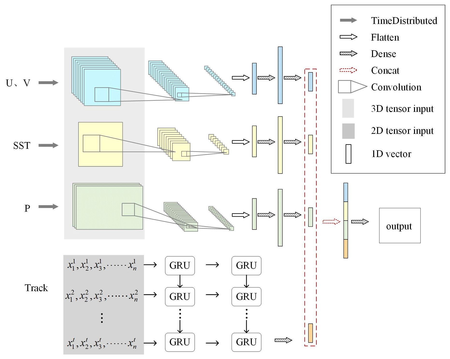
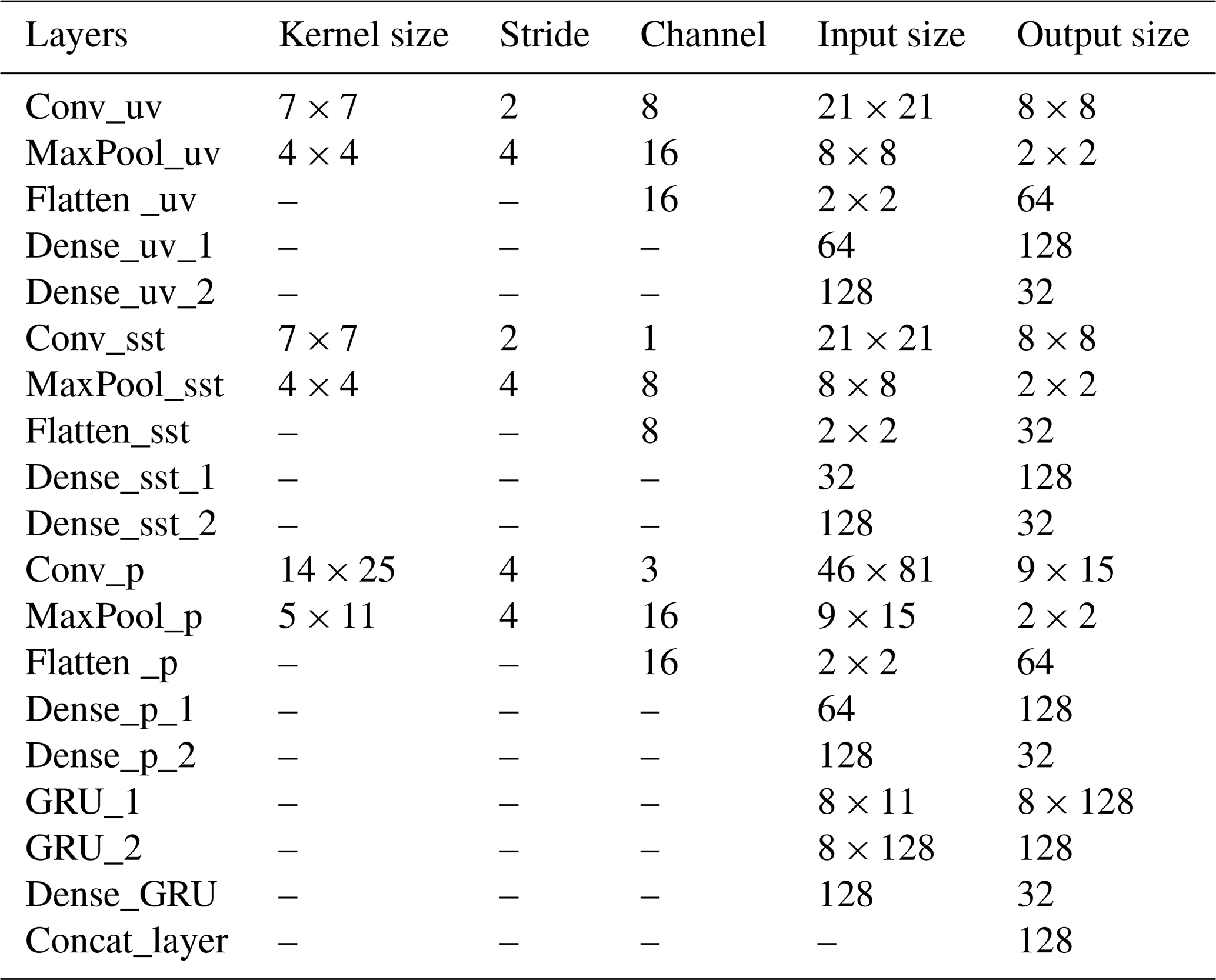
The area of the dark-gray shaded region in Fig. 2 is the two-dimensional trajectory data of the TCs (2D tensor input layer), where represents the input value of the ith feature at the jth timestamp (, ), and they are input into GRU. The model is based on the Adam optimizer and is trained with the RMSE between the forecast and the actual value as a loss function. Due to the different properties among the wind fields, pressure fields, SSTs, and past trajectory data, different learning rates are required for the neural network. Therefore, the parameters of each branch in the model can be trained with the same task, and then the branches can be fused into one network (Concat layer); that is, the dashed red arrow represents the merging of multiple vectors into one vector. It is eventually stitched with output with a fully connected layer; thereafter, the parameters can be adjusted slightly. Table 1 lists the input and output size of each layer in the network framework, including convolution kernel size, stride, and channel number.
Three types of recurrent neural networks (RNN, LSTM, GRU) are used to train samples with eight timestamps and 11 features selected by the random forest method according to their importance; the results of analyzing 49 TCs in 2019–2021 are then evaluated. We set the value of the batch size to 64 and the epoch to 100 and found that the model performed best when the number of neurons in the hidden layer is set to 128; this was determined via experiments using different numbers of neurons in the hidden layer. Early stopping is used to prevent overfitting. When the performance of the model in the validation set begins to decline, training is stopped to avoid overfitting due to continued training.
Table 2Model performance evaluation (RMSE) for RNN, LSTM, and GRU. Bold values highlight the best performance.
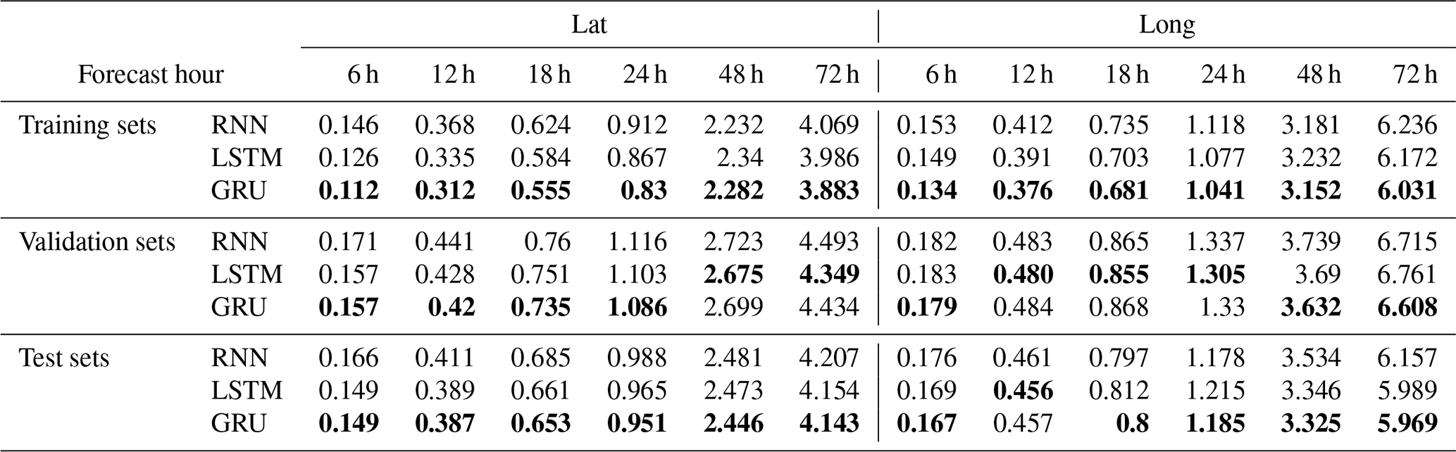
Table 3Comparison of the average absolute distance errors (km) predicted by multiple deep-learning models. Bold values highlight the best performance.
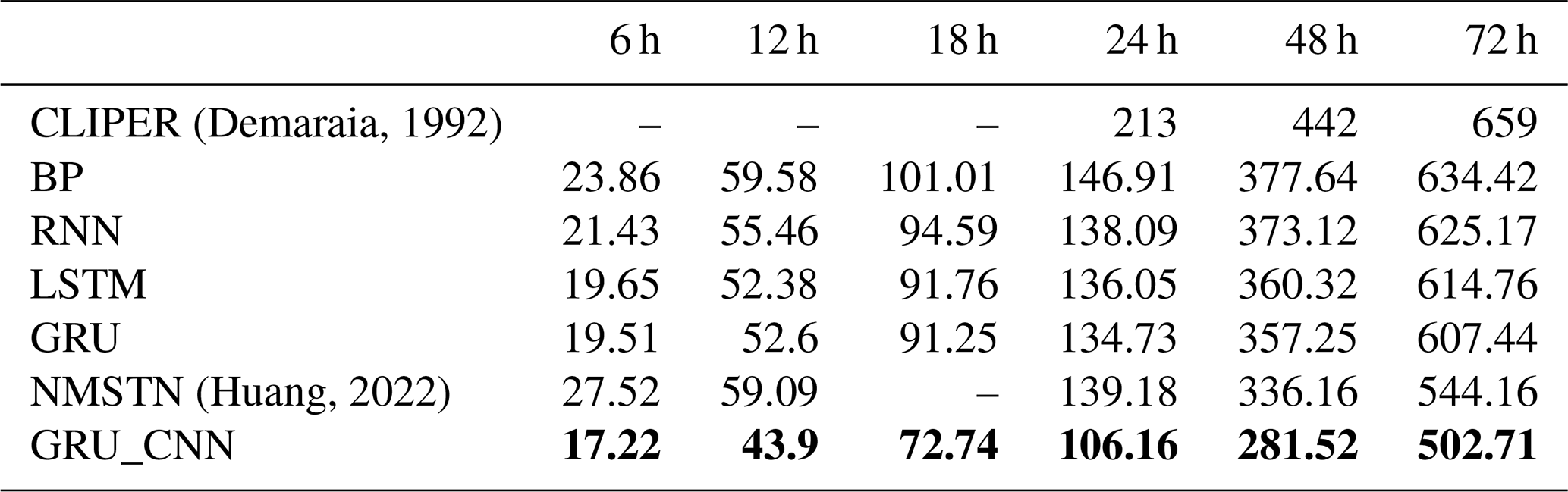
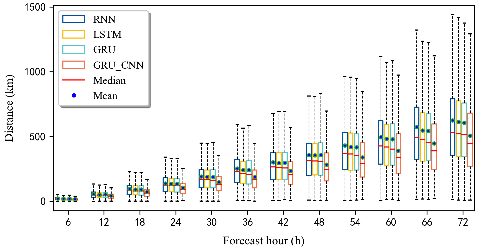
Figure 3The absolute-average-distance boxplot of the three kinds of recurrent neural networks (RNN, LSTM, GRU) and the method in this paper (GRU_CNN) that creates 6–72 h forecasts (intervals of 6 h).
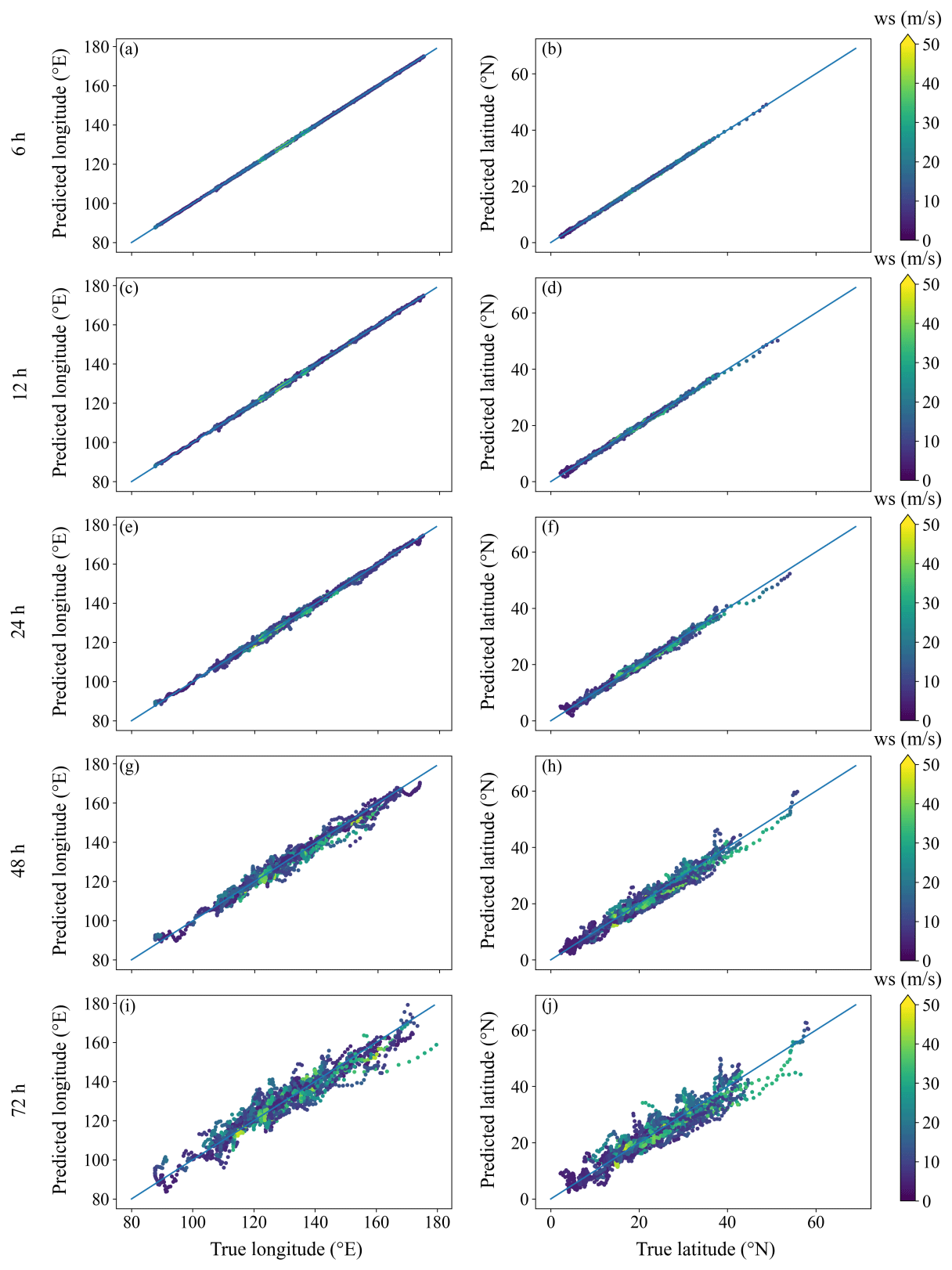
Figure 4Scatter plot distributions of latitude predictions. The color bar represents the maximum wind speed, including the longitude and latitude forecasts at (a, b) 6, (c, d) 12, (e, f) 24, (g, h) 48, and (i, j) 72 h.
The performance evaluation of the three RNN models is displayed in Table 2 by calculating the RMSE values between the predicted longitude (latitude) and the actual longitude (latitude), including the training, validation, and test sets; the best results are highlighted in bold font. It is clear that the GRU-based and LSTM-based models significantly outperformed the RNN-based model, which suggests that the RNN is inferior in handling the problem of long-term dependence. GRU is a variant of LSTM that combines the forget and input gates in LSTM into an update gate and also merges the cell and hidden states. Hence, the parameter amounts of GRU are less than those of LSTM, which results in the overall training speed of GRU being faster than that of LSTM. GRU is theoretically similar to LSTM and can achieve the same accuracy as LSTM (or even better), so the results of GRU and LSTM are close, and their RMSE values are much lower than that of RNN. GRU achieves the best performance in all forecast hours, with the smallest RMSE in the test set. Therefore, we use GRU as a part of the fusion network model called GRU_CNN, adding meteorological environment data processed with CNN.
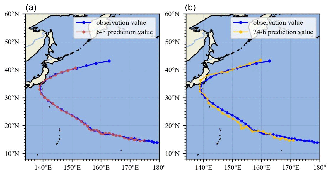
Figure 5Forecast tracks of tropical cyclone FAXAI (2019) – a: 6, b: 24 h.
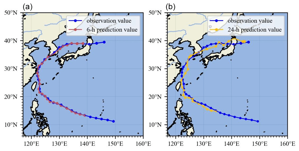
Figure 6Forecast tracks of tropical cyclone MITAG (2019) – a: 6, b: 24 h.
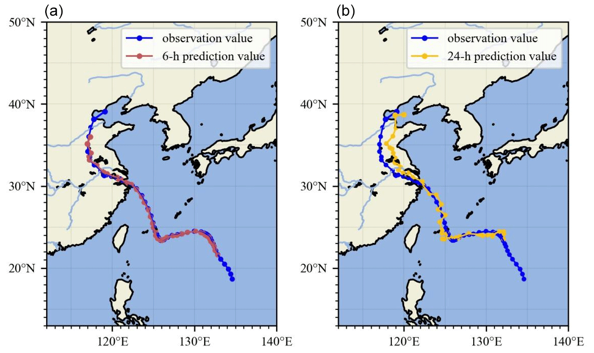
Figure 7Forecast tracks of tropical cyclone IN-FA (2021) – a: 6, b: 24 h.
Table 3 compares the results between GRU_CNN and various deep-learning models, showing the forecast results in the form of the mean absolute distance error. It is evident that GRU_CNN presents an absolute advantage in long-term forecasting. Both LSTM and GRU retain important features through various gate functions, which ensures that they will not be lost during long-term propagation. They can better predict the medium- and long-term tracks of the TCs compared with standard RNNs and two traditional methods named CLIPER and BP. The GRU_CNN is more accurate than the models without CNN. The average distance errors at 6, 24, 48, and 72 h are 17.22, 106.16, 281.52, and 502.71 km, respectively. The error is also reduced compared with the NMSTN method proposed by Huang et al. (2022). In addition, although there is a big difference between the long-term forecast and the numerical prediction results, the average distance prediction results are better than the results provided by the Central Meteorological Observatory (CMO) in the short-term forecasts, including the 6 h (27.57 km) and 12 h (59.09 km) forecasts.
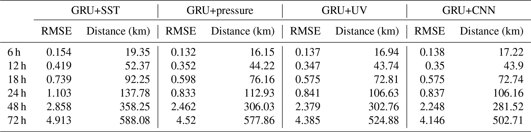
Table 4Comparison of trajectory data combining different environmental features. RMSE is the root mean square error of latitude and longitude, and the distance is the average absolute distance error (km).
As shown in Fig. 3, the maximum distance errors predicted by the three RNNs at 48 and 72 h are over 500 and 1000 km, respectively. Only considering the trajectory characteristics of the TCs in the RNN while ignoring the external atmospheric environmental characteristics will cause instability in the prediction of the TC tracks. The errors of the maximum and average values predicted by the GRU_CNN model are both significantly reduced. To illustrate GRU_CNN more comprehensively and intuitively, Fig. 4 shows a scatter plot of the predicted and actual values. The distance between the data points and the diagonal line represents the prediction error. The higher the wind speed, the stronger the intensity of the TCs, and the closer the predicted value is to the actual value. In addition, with the increase in the forecast time, in high-latitude and high-longitude forecasts when the TC is moving towards the northwest, the predicted value is often lower than the actual value.
Data from three environmental fields are used in this paper: SST, geopotential height (pressure), and wind field (u and v component) data. Different environmental input variables show different effects in the model (Table 4). GRU+SST (pressure, UV) represents only the combination of the trajectory characteristics and SST (geopotential height, wind field), while GRU+CNN is the result of the fusion of the three. The results in Table 4 indicate that GRU+UV performed best, followed by GRU+pressure and then GRU+SST, indicating that the steering flow plays a dominant role in TC forecasting, especially in the short-term <24 h forecast. The forecasting results from adding only the steering flow are close to those of GRU_CNN, while the results at 48 and 72 h illustrate that the influence of the SST and geopotential height on the long-term TC forecast track gradually increases.
To better show the model forecast of GRU_CNN, Figs. 5–7 present the observed and forecast tracks at 6 and 24 h of TCs FAXAI, MITAG, and IN-FA, respectively, and the forecast tracks of other TCs in the test set are presented in Figs. S1–S51 in the Supplement. The blue lines represent the observed tracks, while the red and yellow lines indicate the 6 and 24 h forecast tracks. In general, it is particularly hard to forecast unexpected turns in the TC track. The three TCs shown all exhibit a sudden northward or northwestern turn in the TC track. For the 6 h forecast, the predicted path is approximately consistent with the actual track, while the 24 h forecast has some deviations. The average distance predicted near the northwest turn of FAXAI is 91.35 km; the error for MITAG's first turn to the north is 127.02 km, and the error for the second turn to the northwest is 121.91 km. The two average errors in the track forecast for IN-FA are 84.27 and 82.37 km. It can be seen that there is no significant deviation in the forecast around the steering point; but, for some abnormal track changes, such as crossing back over the same location, samples with more significant errors will be generated, reducing the overall average absolute distance error.
The past 24 h TC trajectory and meteorological field data have been used to forecast TC tracks in the northwestern Pacific from hours 6–72 using deep-learning methods. First, in order to eliminate data redundancy and to reduce the complexity of the prediction model, the random forest algorithm was used for feature extraction of the two-dimensional movement data. Second, three kinds of recurrent neural networks (RNN, LSTM, GRU) were used to evaluate and compare the models based on the input of trajectory features, and it was concluded that GRU performed relatively better in predicting TC tracks. Eventually, we combined GRU with CNN by adding the pre-processed meteorological environmental data around the cyclones (removing the vortex to obtain the steering flow); the CNN models the selected meteorological variables and extracts features, while GRU processes trajectory sequences. GRU_CNN has better prediction results than traditional single deep-learning methods do.
When a new TC generates in the ocean, the GRU_CNN model can quickly provide the forecast track within seconds. Short-term predictions within 12 h of initialization can provide better results than CMO can, and the average distance errors of the forecasts at 6 and 12 h are 17.22 and 43.9 km. When the forecast goes beyond 24 h, the model's accuracy declines. The historical steering flow of cyclones has a significant effect on improving the accuracy of short-term forecasting, while, in long-term forecasting, the SST and geopotential height will have a particular impact, which is regarded as a crucial way of expanding and improving the application of deep-learning models in TC track forecasting. In addition, the model can accurately predict TCs that suddenly turn to the north or northwest, but there will be a considerable distance error for abnormal trajectories, possibly due to a lack of synoptic analysis in our study.
Cyclone prediction has been a challenge in weather forecasting for a long time. With future scientific and technological advances, it is becoming increasingly convenient to obtain meteorological data, and the database has gradually expanded. At the same time, deep-learning models are flexible and can easily be expanded upon. In the future, more data can be integrated, and more valuable features can be extracted to improve the prediction accuracy of the deep-learning model. In addition, model predictor variables will be considered in future work, the inclusion of which can enable the prediction of more useful information, such as cyclone intensity, rainfall, and wind speed.
The code and model are available as a free-access repository on Zenodo at https://doi.org/10.5281/zenodo.7454324 (Wang, 2022).
IBTrACS, which we used in this study, is publicly available. It can be downloaded at https://www.ncei.noaa.gov/data/international-best-track-archive-for-climate-stewardship-ibtracs/v04r00/access/netcdf/IBTrACS.WP.v04r00.nc (NOAA, 2009). ERA5 data can be obtained from the Copernicus Climate Data Store (https://cds.climate.copernicus.eu (Climate Data Store, 2018).
The supplement related to this article is available online at: https://doi.org/10.5194/gmd-16-2167-2023-supplement.
LW wrote the paper and conducted most of the code implementation and data analysis. BW designed the research framework. SZ provided the code and revised the paper. HS was involved in data collation, and ZG was responsible for supervision.
The contact author has declared that none of the authors has any competing interests.
Publisher's note: Copernicus Publications remains neutral with regard to jurisdictional claims in published maps and institutional affiliations.
This study was supported by the National Key Research and Development Program of the Ministry of Science and Technology of China, and by the National Natural Science Foundation of China. We are very grateful to the anonymous reviewers for their careful review and valuable comments, which led to the substantial improvement of this paper.
This research has been supported by the National Key Research and Development Program of the Ministry of Science and Technology of China (grant no. 2018YFC1506405) and by the National Natural Science Foundation of China (grant nos. 42175082 and 42222503).
This paper was edited by Chanh Kieu and reviewed by two anonymous referees.
Alemany, S., Beltran, J., Perez, A., and Ganzfried, S.: Predicting Hurricane Trajectories Using a Recurrent Neural Network, in: Proceedings of the AAAI Conference on Artificial Intelligence, 2–7 February 2018, Lousiana, USA, 33, 468–475, https://doi.org/10.1609/aaai.v33i01.3301468, 2018.
Ali, M. M., Kishtawal, C. M., and Jain, S.: Predicting cyclone tracks in the north Indian Ocean: An artificial neural network approach, Geophys. Res. Lett., 34, 545–559, https://doi.org/10.1029/2006gl028353, 2007.
Bathla, G.: Stock Price prediction using LSTM and SVR, 2020 Sixth International Conference on Parallel, Distributed and Grid Computing (PDGC), 6–8 November 2020, Himachal Pradesh, India, 211–214, https://doi.org/10.1109/PDGC50313.2020.9315800, 2020.
Boussioux, L., Zeng, C., Guenais, T., and Bertsimas, D.: Hurricane Forecasting: A Novel Multimodal Machine Learning Framework, Weather Forecast., 37, 817–831, https://doi.org/10.1175/WAF-D-21-0091.1, 2022.
Brand, S., Buenafe, C. A., and Hamilton, H. D.: Comparison of Tropical Cyclone Motion and Environmental Steering, Mon. Weather Rev., 109, 908–909, https://doi.org/10.1175/1520-0493(1981)109<0908:cotcma>2.0.co;2, 1981.
Chan, J. and Kepert, J.: Global Perspectives on Tropical Cyclones: From Science to Mitigation, in: World Scientific Series on Asia-Pacific Weather and Climate, World Scientific, 4, 448 pp., https://doi.org/10.1142/7597, 2010.
Chan, J. C.-L.: An Observational Study of the Physical Processes Responsible for Tropical Cyclone Motion, J. Atmos. Sci., 41, 1036–1048, https://doi.org/10.1175/1520-0469(1984)041<1036:aosotp>2.0.co;2, 1984.
Chan, J. C. L., Gray, W. M., and Kidder, S. Q.: Forecasting Tropical Cyclone Turning Motion from Surrounding Wind and Temperature Fields, Mon. Weather Rev., 108, 778–792, https://doi.org/10.1175/1520-0493(1980)108<0778:FTCTMF>2.0.CO;2, 1980.
Cho, K., van Merriënboer, B., Gulcehre, C., Bahdanau, D., Bougares, F., Schwenk, H., and Bengio, Y.: Learning Phrase Representations using RNN Encoder–Decoder for Statistical Machine Translation, in: Proceedings of the 2014 Conference on Empirical Methods in Natural Language Processing (EMNLP), 25–29 October 2014, Doha, Qatar, 1724–1734, https://doi.org/10.3115/v1/D14-1179, 2014.
Climate Data Store: Welcome to the Climate Data Store, https://cds.climate.copernicus.eu (last access: 20 April 2023), 2018.
Díaz-Uriarte, R. and Alvarez de Andrés, S.: Gene selection and classification of microarray data using random forest, BMC Bioinformatics, 7, 3, https://doi.org/10.1186/1471-2105-7-3, 2006.
Emanuel, K.: Will Global Warming Make Hurricane Forecasting More Difficult?, B. Am. Meteorol. Soc., 98, 495–501, https://doi.org/10.1175/bams-d-16-0134.1, 2017.
Galarneau, T. J. and Davis, C. A.: Diagnosing Forecast Errors in Tropical Cyclone Motion, Mon. Weather Rev., 141, 405–430, https://doi.org/10.1175/mwr-d-12-00071.1, 2013.
Gao, S., Zhao, P., Pan, B., Li, Y., Zhou, M., Xu, J., Zhong, S., and Shi, Z.: A nowcasting model for the prediction of typhoon tracks based on a long short term memory neural network, Acta Oceanol. Sin., 37, 8–12, https://doi.org/10.1007/s13131-018-1219-z, 2018.
Genuer, R., Poggi, J.-M., and Tuleau-Malot, C.: Variable selection using random forests, Pattern Recogn. Lett., 31, 2225–2236, https://doi.org/10.1016/j.patrec.2010.03.014, 2010.
George, J. E. and Gray, W. M.: Tropical Cyclone Motion and Surrounding Parameter Relationships, J. Appl. Meteorol. Clim., 15, 1252–1264, https://doi.org/10.1175/1520-0450(1976)015<1252:TCMASP>2.0.CO;2, 1976.
Giffard-Roisin, S., Yang, M., Charpiat, G., Kégl, B., and Monteleoni, C.: Fused Deep Learning for Hurricane Track Forecast from Reanalysis Data, Climate Informatics Workshop Proceedings 2018, Boulder, United States, 19 September 2018, https://hal.science/hal-01851001 (last access: 21 September 2018), 69–72, 2018.
Giffard-Roisin, S., Yang, M., Charpiat, G., Kumler Bonfanti, C., Kégl, B., and Monteleoni, C.: Tropical Cyclone Track Forecasting Using Fused Deep Learning From Aligned Reanalysis Data, Front. Big Data, 3, 1, https://doi.org/10.3389/fdata.2020.00001, 2020.
Goerss, J. S.: Tropical Cyclone Track Forecasts Using an Ensemble of Dynamical Models, Mon. Weather Rev., 128, 1187–1193, https://doi.org/10.1175/1520-0493(2000)128<1187:tctfua>2.0.co;2, 2000.
Goldenberg, S. B., Landsea, C. W., Mestas-Nuñez, A. M., and Gray, W. M.: The Recent Increase in Atlantic Hurricane Activity: Causes and Implications, Science, 293, 474–479, https://doi.org/10.1126/science.1060040, 2001.
Graves, A., Jaitly, N., and Mohamed, A.: Hybrid speech recognition with Deep Bidirectional LSTM, 2013 IEEE Workshop on Automatic Speech Recognition and Understanding, 8–12 December 2013, Olomouc, Czech Republic, 273–278, https://doi.org/10.1109/ASRU.2013.6707742, 2013.
Gray, W. M.: Global View of the Origin of Tropical Disturbances and Storms, Mon. Weather Rev., 96, 669–700, https://doi.org/10.1175/1520-0493(1968)096<0669:GVOTOO>2.0.CO;2, 1968.
Hochreiter, S. and Schmidhuber, J.: Long short-term memory, Neural Comput., 9, 1735–1780, https://doi.org/10.1162/neco.1997.9.8.1735, 1997.
Holland, G. J.: Tropical Cyclone Motion: Environmental Interaction Plus a Beta Effect, J. Atmos. Sci., 40, 328–342, https://doi.org/10.1175/1520-0469(1983)040<0328:tcmeip>2.0.co;2, 1983.
Holland, G. J.: Tropical Cyclone Motion. A Comparison of Theory and Observation, J. Atmos. Sci., 41, 68–75, https://doi.org/10.1175/1520-0469(1984)041<0068:tcmaco>2.0.co;2, 1984.
Huang, C., Bai, C., Chan, S., and Zhang, J.: MMSTN: A Multi-Modal Spatial-Temporal Network for Tropical Cyclone Short-Term Prediction, Geophys. Res. Lett., 49, e2021GL096898, https://doi.org/10.1029/2021gl096898, 2022.
Ioffe, S. and Szegedy, C.: Batch Normalization: Accelerating Deep Network Training by Reducing Internal Covariate Shift, in: Proceedings of the 32nd International Conference on International Conference on Machine Learning, The 32nd International Conference on Machine Learning, 6–11 July 2015, Lille, France, 37, 448–456, https://doi.org/10.48550/arXiv.1502.03167, 2015.
Katsube, K. and Inatsu, M.: Response of Tropical Cyclone Tracks to Sea Surface Temperature in the Western North Pacific, J. Climate, 29, 1955–1975, https://doi.org/10.1175/jcli-d-15-0198.1, 2016.
Kim, S., Kang, J.-S., Lee, M., and Song, S.-K.: DeepTC: ConvLSTM Network for Trajectory Prediction of Tropical Cyclone using Spatiotemporal Atmospheric Simulation Data, in: Spatiotemporal Workshop at 31st Conference on Neural Information Processing Systems, 2–8 December 2018, Montréal, Canada, https://openreview.net/pdf?id=HJlCVoPAF7 (last access: 20 April 2023), 2018.
Kitade, T.: A Numerical Study of the Vortex Motion with Barotropic Models, J. Meteorol. Soc. Jpn. Ser. II, 59, 801–807, https://doi.org/10.2151/jmsj1965.59.6_801, 1981.
Klein, B., Wolf, L., and Afek, Y.: A Dynamic Convolutional Layer for short rangeweather prediction, in: 2015 IEEE Conference on Computer Vision and Pattern Recognition (CVPR), 7–12 June 2015, Boston, US, 4840–4848, https://doi.org/10.1109/CVPR.2015.7299117, 2015.
Krizhevsky, A., Sutskever, I., and Hinton, G.: ImageNet Classification with Deep Convolutional Neural Networks, Neural Information Processing Systems, 3–6 December 2012, Nevada, USA, 25, 84–90, https://doi.org/10.1145/3065386, 2012.
Lecun, Y., Bottou, L., Bengio, Y., and Haffner, P.: Gradient-Based Learning Applied to Document Recognition, P. IEEE, 86, 2278–2324, https://doi.org/10.1109/5.726791, 1998.
Li-min, S., Gang, F. U., Xiang-chun, C., and Jian, Z.: Application of BP neural network to forecasting typhoon tracks, Journal of Natural Disasters, 18, 104–111, https://doi.org/10.3969/j.issn.1004-4574.2009.06.018, 2009.
Liu, H., Mi, X., and Li, Y.: Smart multi-step deep learning model for wind speed forecasting based on variational mode decomposition, singular spectrum analysis, LSTM network and ELM, Energ. Convers. Manage., 159, 54–64, https://doi.org/10.1016/j.enconman.2018.01.010, 2018.
Liu, Z., Hao, K., Geng, X., Zou, Z., and Shi, Z.: Dual-Branched Spatio-Temporal Fusion Network for Multihorizon Tropical Cyclone Track Forecast, IEEE J. Sel. Top. Appl., 15, 3842–3852, https://doi.org/10.1109/JSTARS.2022.3170299, 2022.
Lownam, C.: The NCAR-AFWA tropical cyclone bogussing scheme. A report prepared for the Air Force Weather Agency (AFWA), National Center for Atmospheric Research, https://citeseerx.ist.psu.edu/document?repid=rep1&type=pdf&doi=45979165eea27836ac82671f2e5dedb275eabcab (last access: 20 April 2023), 2001.
Moradi Kordmahalleh, M., Gorji Sefidmazgi, M., Homaifar, A., and Liess, S.: Hurricane Trajectory Prediction Via a Sparse Recurrent Neural Network, in: Proceedings of the 5th International Workshop on Climate Informatics, 19–21 September 2015, Boulder, USA, 2–3, https://www.researchgate.net/publication/320456406_Hurricane_Trajectory_Prediction_Via_a_Sparse_Recurrent_Neural_Network (last access: 20 April 2023), 2015.
Neumann, C. J. and Hope, J. R.: Performance Analysis of the HURRAN Tropical Cyclone Forecast System, Mon. Weather Rev., 100, 245–255, https://doi.org/10.1175/1520-0493(1972)100<0245:paotht>2.3.co;2, 1972.
NOAA: Index of /data/international-best-track-archive-for-climate-stewardship-ibtracs/v04r00, https://www.ncei.noaa.gov/data/international-best-track-archive-for-climate-stewardship-ibtracs/v04r00/access/netcdf/IBTrACS.WP.v04r00.nc (last access: 20 April 2023), 2009.
Ortega, L. C., Otero, L. D., Solomon, M., Otero, C. E., and Fabregas, A.: Deep learning models for visibility forecasting using climatological data, Int. J. Forecasting, 39, 992–1004, https://doi.org/10.1016/j.ijforecast.2022.03.009, 2022.
Roy, C. and Kovordányi, R.: Tropical cyclone track forecasting techniques – A review, Atmos. Res., 104–105, 40–69, https://doi.org/10.1016/j.atmosres.2011.09.012, 2012.
Ruttgers, M., Lee, S., Jeon, S., and You, D.: Prediction of a typhoon track using a generative adversarial network and satellite images, Sci. Rep.-UK, 9, 6057, https://doi.org/10.1038/s41598-019-42339-y, 2019.
Schulthess, T. C., Bauer, P., Wedi, N., Fuhrer, O., Hoefler, T., and Schär, C.: Reflecting on the Goal and Baseline for Exascale Computing: A Roadmap Based on Weather and Climate Simulations, Comput. Sci. Eng., 21, 30–41, https://doi.org/10.1109/MCSE.2018.2888788, 2019.
Shi, X., Chen, Z., Wang, H., Yeung, D.-Y., Wong, W. K., and Woo, W.-C.: Convolutional LSTM Network: A Machine Learning Approach for Precipitation Nowcasting, in: Proceedings of the 28th International Conference on Neural Information Processing Systems, 7–12 December 2015, Montreal, Canada, 1, 802–810, https://doi.org/10.48550/arXiv.1506.04214, 2015.
Sun, Y., Zhong, Z., Li, T., Yi, L., Camargo, S. J., Hu, Y., Liu, K., Chen, H., Liao, Q., and Shi, J.: Impact of ocean warming on tropical cyclone track over the western north pacific: A numerical investigation based on two case studies, J. Geophys. Res.-Atmos., 122, 8617–8630, https://doi.org/10.1002/2017JD026959, 2017.
Wang, C. and Fu, Y.: Ship Trajectory Prediction Based on Attention in Bidirectional Recurrent Neural Networks, in: 2020 5th International Conference on Information Science, Computer Technology and Transportation (ISCTT), 13–15 November 2020, Shenyang, China, 529–533, https://doi.org/10.1109/isctt51595.2020.00100, 2020.
Wang, L.: Hush980/TCs_DL_code: Second release of my code (v2.0.0), Zenodo [code], https://doi.org/10.5281/zenodo.7454324, 2022.
Wang, Y., Zhang, W., and Fu, W.: Back Propogation(BP)-neural network for tropical cyclone track forecast, Proceedings – 2011 19th International Conference on Geoinformatics, Geoinformatics 2011, 24–26 June 2011, Shanghai, China, 1–4, https://doi.org/10.1109/GeoInformatics.2011.5981095, 2011.
Zhang, Y., Chandra, R., and Gao, J.: Cyclone Track Prediction with Matrix Neural Networks, 2018 International Joint Conference on Neural Networks (IJCNN), 8–13 July 2018, Rio, Brazil, 1–8, https://doi.org/10.1109/IJCNN.2018.8489077, 2018.