Causal deep learning models for studying the Earth system

Earth is a complex non-linear dynamical system. Despite decades of research and considerable scientific and methodological progress, many processes and relations between Earth system variables remain poorly understood. Current approaches for studying relations in the Earth system rely either on numerical simulations or statistical approaches. However, there are several inherent limitations to existing approaches, including high computational costs, uncertainties in numerical models, strong assumptions about linearity or locality, and the fallacy of correlation and causality. Here, we propose a novel methodology combining deep learning (DL) and principles of causality research in an attempt to overcome these limitations. On the one hand, we employ the recent idea of training and analyzing DL models to gain new scientific insights into relations between input and target variables. On the other hand, we use the fact that a statistical model learns the causal effect of an input variable on a target variable if suitable additional input variables are included. As an illustrative example, we apply the methodology to study soil-moisture–precipitation coupling in ERA5 climate reanalysis data across Europe. We demonstrate that, harnessing the great power and flexibility of DL models, the proposed methodology may yield new scientific insights into complex non-linear and non-local coupling mechanisms in the Earth system.

1 Introduction

The Earth system comprises many complex processes and non-linear relations between variables that are still not fully understood. Considering, for example, soil-moisture–precipitation coupling, i.e., the question of how precipitation changes if soil moisture is changed, it is well known that soil moisture affects the temperature and humidity profile of the atmosphere and thereby influences the development and onset of precipitation (Seneviratne et al., 2010; Santanello et al., 2018). However, because there are several concurring pathways of soil-moisture–precipitation coupling, it remains an open question whether an increase in soil moisture leads to an increase or decrease in precipitation. Answering this question might lead to improved precipitation predictions with numerical models.

Approaches for studying relations in the Earth system may be broadly divided into approaches based on numerical simulations (e.g., Koster, 2004; Seneviratne et al., 2006; Hartick et al., 2021) and statistical approaches (e.g., Taylor, 2015; Guillod et al., 2015; Tuttle and Salvucci, 2016). Both classes of approaches have several inherent limitations. Approaches based on numerical simulations usually have high computational costs and, even more importantly, rely on the correct representation of the considered relations in the numerical model. For example, precipitation in numerical models lacks accuracy due to several simplified parameterizations; thus, using these models to study soil-moisture–precipitation coupling is problematic. On the other hand, statistical approaches usually have much lower computational costs and can directly be applied to observational data. However, current statistical approaches have strong limitations on their own, for example, due to assumptions on linearity or locality of considered relations and negligence of the difference between causality and correlation.

A recent statistical approach for studying relations in the Earth system is to (i) train deep learning (DL) models to predict one Earth system variable given one or several others and (ii) use methods from the realm of interpretable DL (Zhang and Zhu, 2018; Montavon et al., 2018; Gilpin et al., 2018; Molnar, 2019; Samek et al., 2021) to analyze the relations learned by the models (Roscher et al., 2020). The approach has been applied in several recent studies (Ham et al., 2019; Gagne et al., 2019; McGovern et al., 2019; Toms et al., 2020; Ebert-Uphoff and Hilburn, 2020; Padarian et al., 2020), and the use of DL models allows us to overcome common assumptions in other statistical approaches like linearity or locality. So far, however, the difference between causality and correlation has been neglected in studies using this approach. Indeed, DL models might learn various (spurious) correlations between input and target variables, while researchers striving for new scientific insights are most interested in causal relations.

Therefore, in this work, we propose extending the approach by combining it with a result from causality research stating that a statistical model may learn the causal effect of an input variable on a target variable if suitable additional input variables are included (Pearl, 2009; Shpitser et al., 2010). In the geosciences, this result has only recently received attention in the work of Massmann et al. (2021). In this work, it is combined with the methodology of training and analyzing DL models to gain new scientific insights for the first time. Note that there are several other recent studies on causal inference methods in the geosciences (e.g., Tuttle and Salvucci, 2016, 2017; Ebert-Uphoff and Deng, 2017; Green et al., 2017; Runge, 2018; Runge et al., 2019; Barnes et al., 2019; Massmann et al., 2021). However, most of them focus on discovering causal dependencies between variables, while the proposed methodology assumes prior knowledge on causal dependencies and focuses on quantifying the strength and sign of a particular causal dependency. As an illustrative example, we apply the proposed methodology to study soil-moisture–precipitation coupling in ERA5 climate reanalysis data across Europe. Other geoscientific questions that could be addressed with the proposed methodology are, for example, soil-moisture–temperature coupling (Seneviratne et al., 2006; Schwingshackl et al., 2017; Schumacher et al., 2019) and soil-moisture–atmospheric-carbon-dioxide coupling (Green et al., 2019; Humphrey et al., 2021).

This paper is structured as follows: Section 2 introduces the background on causality research and details the proposed methodology. Section 3 presents the application to soil-moisture–precipitation coupling and provides a comparison to other approaches. Finally, Sect. 4 contains several additional analyses to assess the statistical significance and correctness of results obtained with the proposed methodology.

2 Methodology

To introduce the proposed methodology, which combines deep learning with a result from causality research, we first give a basic introduction into the required concepts from causality research. Based on that, we describe how one can train a DL model that reflects causality.

2.1 Background on causality

If we could change the value of any Earth system variable, e.g., increase soil moisture in some area, this would potentially affect numerous other Earth system variables, e.g., evaporation, temperature and precipitation. The variable that was changed thus has a causal impact on the latter variables. Formally, the causal effect of some variable X∈ℝ^d on another variable Y∈ℝⁿ is the expected response of Y to changing the value of X. To determine this impact, one has to determine the expected value of Y given that one sets X to some arbitrary value x. In the framework of structural causal models (SCMs) introduced below, setting X to x is represented by a mathematical intervention operator do(X=x), and the sought value is referred to as the post-intervention expected value $\mathbb{E}\left[\mathit{Y}\right|\mathrm{do}(\mathit{X}=\mathit{x})]$.

In some cases, $\mathbb{E}\left[\mathit{Y}\right|\mathrm{do}(\mathit{X}=\mathit{x})]$ can be determined experimentally by setting X to x while monitoring Y. For example, in Earth System Modeling, one may be able to set X to x in numerical experiments. However, often it is impossible to determine $\mathbb{E}\left[\mathit{Y}\right|\mathrm{do}(\mathit{X}=\mathit{x})]$ experimentally due to computational constraints or because of the lack of appropriate numerical models. Obviously, analog experiments are even harder to perform or impossible in case of large-scale interactions in the Earth system.

The framework of SCMs (Pearl, 2009) provides a deeper understanding of the notion $\mathbb{E}\left[\mathit{Y}\right|\mathrm{do}(\mathit{X}=\mathit{x})]$ and describes how it can be determined without experimentally setting X to x. The framework is briefly introduced in the following. For a more in-depth introduction we refer to Pearl (2009). An introduction to the framework in the context of geosciences is given in Massmann et al. (2021).

2.1.1 Structural causal models

In the framework of SCMs, the considered system, e.g., the Earth system, is described by a causal graph and associated structural equations. A causal graph is a directed acyclic graph, in which nodes represent the variables of the system and edges encode the dependencies between these variables. For example, in the system described by Fig. 1a, variable Y depends on all other variables, although the lack of an edge from X to Y implies that X only affects Y indirectly via its impact on C₂. Parents of a considered variable (node) are all variables that have a direct effect on that variable, i.e., all variables with an edge pointing to that variable. In the following, the terms “node” and “variable” are used interchangeably.

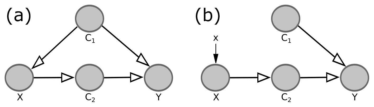
Figure 1 Example for a causal graph (a) and corresponding causal graph for setting variable X to some arbitrary value x (b). The grey circles are referred to as nodes of the graph, while the arrows are referred to as directed edges.

Formally, a variable in the causal graph is determined by a function f, whose inputs are its parents and a random variable U representing potential chaos and variables not included in the causal graph explicitly. For example, for the system in Fig. 1a, the four variables are determined by four functions $f_{C_{\mathrm{1}}},f_{C_{\mathrm{2}}},f_X,f_Y$:

$$\begin{array}{}\text{(1)}& \begin{array}{rl}{\mathit{C}}_{\mathrm{1}}& =f_{C_{\mathrm{1}}}\left({\mathit{U}}_{C_{\mathrm{1}}}\right),\mathit{X}=f_X({\mathit{C}}_{\mathrm{1}},{\mathit{U}}_X),\\ {\mathit{C}}_{\mathrm{2}}& =f_{C_{\mathrm{2}}}(\mathit{X},{\mathit{U}}_{C_{\mathrm{2}}}),\mathit{Y}=f_Y({\mathit{C}}_{\mathrm{1}},{\mathit{C}}_{\mathrm{2}},{\mathit{U}}_Y).\end{array}\end{array}$$

These equations are called structural equations. The random variables ${\mathit{U}}_{C_{\mathrm{1}}},{\mathit{U}}_{C_{\mathrm{2}}},{\mathit{U}}_X,{\mathit{U}}_Y$ are assumed to be mutually independent and give rise to a probability distribution $\mathbb{P}({\mathit{C}}_{\mathrm{1}},{\mathit{C}}_{\mathrm{2}},\mathit{X},\mathit{Y})$, which describes the probability of observing any tuple of values $({\mathit{c}}_{\mathrm{1}},{\mathit{c}}_{\mathrm{2}},\mathit{x},\mathit{y})$. Integrating the product of Y and this probability distribution over all tuples $({\mathit{c}}_{\mathrm{1}},{\mathit{c}}_{\mathrm{2}},\mathit{y})$ for some fixed value x, one obtains the expected value of Y given that one observes the value x of X, i.e.,

$$\begin{array}{}\text{(2)}& \mathbb{E}\left[\mathit{Y}\right|\mathit{X}=\mathit{x}]=\underset{{\mathit{c}}_{\mathrm{1}},{\mathit{c}}_{\mathrm{2}},\mathit{y}}{\int }\mathit{y}\cdot \mathbb{P}[{\mathit{C}}_{\mathrm{1}}={\mathit{c}}_{\mathrm{1}},{\mathit{C}}_{\mathrm{2}}={\mathit{c}}_{\mathrm{2}},\mathit{Y}=\mathit{y}|\mathit{X}=\mathit{x}].\end{array}$$

As stated above, to determine the causal effect of X on Y, one has to determine the expected value of Y given that one set X to some arbitrary value x, i.e., the post-intervention expected value $\mathbb{E}\left[\mathit{Y}\right|\mathrm{do}(\mathit{X}=\mathit{x})]$. By setting X to some arbitrary value x, all dependencies of X on other variables are eliminated. Within the framework of SCMs, this corresponds to removing all edges in the causal graph pointing to X and modifying the structural equation for X accordingly. For example, when studying the causal effect of X on Y in Fig. 1a, the modified system is described by the causal graph in Fig. 1b with the associated structural equations

$$\begin{array}{}\text{(3)}& \begin{array}{rl}{\mathit{C}}_{\mathrm{1}}& =f_{C_{\mathrm{1}}}\left({\mathit{U}}_{C_{\mathrm{1}}}\right),\mathit{X}=\mathit{x},{\mathit{C}}_{\mathrm{2}}=f_{C_{\mathrm{2}}}(\mathit{X},{\mathit{U}}_{C_{\mathrm{2}}}),\\ \mathit{Y}& =f_Y({\mathit{C}}_{\mathrm{1}},{\mathit{C}}_{\mathrm{2}},{\mathit{U}}_Y).\end{array}\end{array}$$

Again, the random variables ${\mathit{U}}_{C_{\mathrm{1}}},{\mathit{U}}_{C_{\mathrm{2}}},{\mathit{U}}_Y$ give rise to a probability distribution $\mathbb{P}({\mathit{C}}_{\mathrm{1}},{\mathit{C}}_{\mathrm{2}},\mathit{Y}|\mathrm{do}(\mathit{X}=\mathit{x}))$, referred to as the post-intervention probability distribution, and the corresponding post-intervention expected value $\mathbb{E}\left[\mathit{Y}\right|\mathrm{do}(\mathit{X}=\mathit{x})]$. This expected value is used to determine the causal effect of X on Y and differs from the expected value for the original system, $\mathbb{E}\left[\mathit{Y}\right|\mathit{X}=\mathit{x}]$. For instance, in the example from Fig. 1, knowing X allows us to draw conclusions about Y both in the original system (Fig. 1a) and in the modified system (Fig. 1b), because X has a causal effect on Y (via its impact on C₂). However, in the original system, knowing X allows us to draw additional conclusions about C₁. This is the case although the edge in the causal graph points from C₁ to X; i.e., C₁ affects X, not vice versa. For example, if X was simply the sum of C₁ and the random term U_X, a high value of X would probably imply a high value of C₁. These conclusions about C₁ cannot be drawn in the modified system, where the edge from C₁ to X is removed. The knowledge about C₁ allows us to draw further conclusions about Y because C₁ also affects Y. Summarizing, due to the confounding influence of C₁, knowing X reveals more about Y in the original system than in the modified system, which is why the original expected value $\mathbb{E}\left[\mathit{Y}\right|\mathit{X}=\mathit{x}]$ and the post-intervention expected value $\mathbb{E}\left[\mathit{Y}\right|\mathrm{do}(\mathit{X}=\mathit{x})]$ differ.

If we could observe the modified system, i.e., if we could experimentally set variable X to arbitrary values x, we could approximate the post-intervention expected value $\mathbb{E}\left[\mathit{Y}\right|\mathrm{do}(\mathit{X}=\mathit{x})]$ by training a suitable (see Sect. 2.2.1) statistical model on the observed tuples (x,y) to predict Y given X. However, in the cases considered in the proposed methodology, it is impossible or undesirable to experimentally set X to x. Thus, we can only observe the original system and approximate the original expected value $\mathbb{E}\left[\mathit{Y}\right|\mathit{X}=\mathit{x}]$ by analogously training a statistical model on observed tuples (x,y) of the original system. Consequently, we have to bridge the gap between the original expected value $\mathbb{E}\left[\mathit{Y}\right|\mathit{X}=\mathit{x}]$ and the post-intervention expected value $\mathbb{E}\left[\mathit{Y}\right|\mathrm{do}(\mathit{X}=\mathit{x})]$.

2.1.2 Adjustment criteria

To bridge the gap between the original expected value $\mathbb{E}\left[\mathit{Y}\right|\mathit{X}=\mathit{x}]$ and the post-intervention expected value $\mathbb{E}\left[\mathit{Y}\right|\mathrm{do}(\mathit{X}=\mathit{x})]$, we must take into account variables other than X and Y. Indeed, in the example from Fig. 1, we showed that original and post-intervention expected values differ because, in the original system, knowing X allows inferences about C₁ that are not possible in the modified system. However, if we actually knew C₁, this would not be the case; thus, the original expected value $\mathbb{E}\left[\mathit{Y}\right|\mathit{X}=\mathit{x},{\mathit{C}}_{\mathrm{1}}={\mathit{c}}_{\mathrm{1}}]$ and the post-intervention expected value $\mathbb{E}\left[\mathit{Y}\right|\mathrm{do}(\mathit{X}=\mathit{x}),{\mathit{C}}_{\mathrm{1}}={\mathit{c}}_{\mathrm{1}}]$ are identical. Analogously to $\mathbb{E}\left[\mathit{Y}\right|\mathit{X}=\mathit{x}]$, the expected value $\mathbb{E}\left[\mathit{Y}\right|\mathit{X}=\mathit{x},{\mathit{C}}_{\mathrm{1}}={\mathit{c}}_{\mathrm{1}}]$ can be approximated by observing the original system and training a statistical model on the observed tuples $(\mathit{x},\mathit{y},{\mathit{c}}_{\mathrm{1}})$ to predict Y given X and C₁. Therefore, this equality allows us to approximate the post-intervention expected value $\mathbb{E}\left[\mathit{Y}\right|\mathrm{do}(\mathit{X}=\mathit{x}),{\mathit{C}}_{\mathrm{1}}={\mathit{c}}_{\mathrm{1}}]$ by only observing the original system and without experimentally setting X to x.

In the proposed methodology, we exploit the fact that the equality

$$\begin{array}{}\text{(4)}& \begin{array}{rl}\mathbb{E}\left[\mathit{Y}\right|\mathit{X}& =\mathit{x},\mathit{\{}{\mathit{C}}_{\mathrm{\ell }}={\mathit{c}}_{\mathrm{\ell }}{\mathit{\}}}_{\mathrm{\ell }=\mathrm{1}}^k]\\ & =\mathbb{E}\left[\mathit{Y}\right|\mathrm{do}(\mathit{X}=\mathit{x}),\mathit{\{}{\mathit{C}}_{\mathrm{\ell }}={\mathit{c}}_{\mathrm{\ell }}{\mathit{\}}}_{\mathrm{\ell }=\mathrm{1}}^k]\end{array}\end{array}$$

holds for any causal graph, thus allowing us to determine the post-intervention expected value $\mathbb{E}\left[\mathit{Y}\right|\mathrm{do}(\mathit{X}=\mathit{x}),\mathit{\{}{\mathit{C}}_{\mathrm{\ell }}={\mathit{c}}_{\mathrm{\ell }}{\mathit{\}}}_{\mathrm{\ell }=\mathrm{1}}^k]$ from observations alone, if the additional variables ${\mathit{C}}_{\mathrm{\ell }}\in {\mathbb{R}}^{d_{\mathrm{\ell }}},\mathrm{\ell }=\mathrm{1},\mathrm{\dots },k,$ fulfill the following adjustment criteria (Shpitser et al., 2010):

1. the variables $\mathit{\{}{\mathit{C}}_{\mathrm{\ell }}{\mathit{\}}}_{\mathrm{\ell }=\mathrm{1}}^k$ block all non-causal paths from X to Y in the original causal graph;

2. no $\mathit{\{}{\mathit{C}}_{\mathrm{\ell }}{\mathit{\}}}_{\mathrm{\ell }=\mathrm{1}}^k$ lies on a causal path from X to Y.

Here, a path is any consecutive sequence of edges. A path between X and Y is causal from X to Y if all edges point towards Y, and it is non-causal otherwise. A path is blocked by a set $S=\mathit{\{}{\mathit{C}}_{\mathrm{\ell }}{\mathit{\}}}_{\mathrm{\ell }=\mathrm{1}}^k$ of nodes if either (i) the path contains at least one edge-emitting node, i.e., a node with at least one adjacent edge pointing away from the node ($\mathrm{\dots }\leftrightarrow \mathit{C}\to \mathrm{\dots }$), that is in S (e.g., the path $\mathit{X}\leftarrow {\mathit{C}}_{\mathrm{1}}\to \mathit{Y}$ in Fig. 1 is blocked by S if S contains C₁), or (ii) the path contains at least one collision node, i.e., a node with both adjacent edges pointing towards the node ($\mathrm{\dots }\to \mathit{C}\leftarrow \mathrm{\dots }$), which is outside S and has no descendants in S (e.g., the path $\mathit{X}\to \mathit{C}\leftarrow \mathit{Y}$ is blocked if S does not contain C).

The first adjustment criterion generalizes the example of C₁ in Fig. 1, where adjusting for the edge-emitting node C₁, i.e., considering $\mathbb{E}\left[\mathit{Y}\right|\mathit{X}=\mathit{x},{\mathit{C}}_{\mathrm{1}}={\mathit{c}}_{\mathrm{1}}]$ rather than $\mathbb{E}\left[\mathit{Y}\right|\mathit{X}=\mathit{x}]$, blocks the non-causal path $\mathit{X}\leftarrow {\mathit{C}}_{\mathrm{1}}\to \mathit{Y}$ such that X is only used to draw conclusions about Y via the causal path $\mathit{X}\to {\mathit{C}}_{\mathrm{2}}\to \mathit{Y}$. In general, the criterion ensures that X is only used to draw conclusions about Y via causal paths from X to Y and not via any non-causal path between X and Y.

The second adjustment criterion ensures that no causal path from X to Y is blocked, such that the post-intervention expected value $\mathbb{E}\left[\mathit{Y}\right|\mathrm{do}(\mathit{X}=\mathit{x}),\mathit{\{}{\mathit{C}}_{\mathrm{\ell }}={\mathit{c}}_{\mathrm{\ell }}{\mathit{\}}}_{\mathrm{\ell }=\mathrm{1}}^k]$ actually reflects the causal effect of X on Y. For example, considering the causal path $\mathit{X}\to {\mathit{C}}_{\mathrm{2}}\to \mathit{Y}$ in Fig. 1, C₂ blocks the only causal path between X and Y. Thus, $\mathbb{E}\left[\mathit{Y}\right|\mathrm{do}(\mathit{X}=\mathit{x}),{\mathit{C}}_{\mathrm{2}}={\mathit{c}}_{\mathrm{2}}]=\mathbb{E}[\mathit{Y}|{\mathit{C}}_{\mathrm{2}}={\mathit{c}}_{\mathrm{2}}]$ would indicate that there is no causal effect of X on Y.

Summarizing this section, we can approximate the post-intervention expected value $\mathbb{E}\left[\mathit{Y}\right|\mathrm{do}(\mathit{X}=\mathit{x}),\mathit{\{}{\mathit{C}}_{\mathrm{\ell }}={\mathit{c}}_{\mathrm{\ell }}{\mathit{\}}}_{\mathrm{\ell }=\mathrm{1}}^k]$ from observations alone, if we can describe the considered system by a causal graph and find variables ${\mathit{C}}_{\mathrm{\ell }}\in {\mathbb{R}}^{d_{\mathrm{\ell }}},\mathrm{\ell }=\mathrm{1},\mathrm{\dots },k$, that fulfill the above adjustment criteria. Describing the system by a causal graph requires knowledge on which variables are relevant to the considered relation (represented by the nodes in the graph) and on the existence of causal dependencies between these variables (represented by the edges in the graph). Nevertheless, it does not require knowledge on the sign or strength of these dependencies, i.e., on the structural equations. Note that the parents of X in the causal graph always fulfill the adjustment criteria. In the proposed methodology, we exploit the post-intervention expected value $\mathbb{E}\left[\mathit{Y}\right|\mathrm{do}(\mathit{X}=\mathit{x}),\mathit{\{}{\mathit{C}}_{\mathrm{\ell }}={\mathit{c}}_{\mathrm{\ell }}{\mathit{\}}}_{\mathrm{\ell }=\mathrm{1}}^k]$ to determine the causal effect of X on Y as detailed in Sect. 2.2.2.

2.2 Steps of the methodology

The proposed methodology is as follows: given a complex relation between two variables X∈ℝ^d and Y∈ℝⁿ, for example, soil-moisture–precipitation coupling, we train a causal deep learning (DL) model to predict Y given X and additional input variables ${\mathit{C}}_{\mathrm{\ell }}\in {\mathbb{R}}^{d_{\mathrm{\ell }}},\mathrm{\ell }=\mathrm{1},\mathrm{\dots },k$. In a second step, we perform a sensitivity analysis of the trained model to analyze how Y would change if we changed X, i.e., to determine the causal effect of X on Y.

2.2.1 Training a causal DL model

DL models (LeCun et al., 2015; Reichstein et al., 2019) learn statistical associations between their input and target variables. By training a causal DL model, we mean that we train a DL model that approximates for each input tuple $(\mathit{x},\mathit{\{}{\mathit{c}}_{\mathrm{\ell }}{\mathit{\}}}_{\mathrm{\ell }=\mathrm{1}}^k)$ the post-intervention expected value $\mathbb{E}\left[\mathit{Y}\right|\mathrm{do}(\mathit{X}=\mathit{x}),\mathit{\{}{\mathit{C}}_{\mathrm{\ell }}={\mathit{c}}_{\mathrm{\ell }}{\mathit{\}}}_{\mathrm{\ell }=\mathrm{1}}^k]$, i.e., the model approximates the map

$$\begin{array}{}\text{(5)}& (\mathit{x},\mathit{\{}{\mathit{c}}_{\mathrm{\ell }}{\mathit{\}}}_{\mathrm{\ell }=\mathrm{1}}^k)\to \mathbb{E}[\mathit{Y}\left|\mathrm{do}\right(\mathit{X}=\mathit{x}),\mathit{\{}{\mathit{C}}_{\mathrm{\ell }}={\mathit{c}}_{\mathrm{\ell }}{\mathit{\}}}_{\mathrm{\ell }=\mathrm{1}}^k].\end{array}$$

To obtain a causal DL model, the loss function, model architecture and additional input variables $\mathit{\{}{\mathit{C}}_{\mathrm{\ell }}{\mathit{\}}}_{\mathrm{\ell }=\mathrm{1}}^k$ have to be chosen carefully. In particular, we choose a loss function that is minimized by the original expected value of Y given X and the other input variables, i.e., by the map

$$\begin{array}{}\text{(6)}& (\mathit{x},\mathit{\{}{\mathit{c}}_{\mathrm{\ell }}{\mathit{\}}}_{\mathrm{\ell }=\mathrm{1}}^k)\to \mathbb{E}[\mathit{Y}|\mathit{X}=\mathit{x},\mathit{\{}{\mathit{C}}_{\mathrm{\ell }}={\mathit{c}}_{\mathrm{\ell }}{\mathit{\}}}_{\mathrm{\ell }=\mathrm{1}}^k].\end{array}$$

An example for such a loss function is the expected mean squared error,

$$\begin{array}{}\text{(7)}& (\mathit{m}:(\mathit{X},\mathit{\left\{}{\mathit{C}}_{\mathrm{\ell }}{\mathit{\}}}_{\mathrm{\ell }=\mathrm{1}}^k\right)\to {\mathbb{R}}^n)\to \mathbb{E}[(\mathit{Y}-\mathit{m}(\mathit{x},\mathit{\left\{}{\mathit{c}}_{\mathrm{\ell }}{\mathit{\}}}_{\mathrm{\ell }=\mathrm{1}}^k\right){)}^{\mathrm{2}}],\end{array}$$

which maps a function $\mathit{m}:(\mathit{X},\mathit{\{}{\mathit{C}}_{\mathrm{\ell }}{\mathit{\}}}_{\mathrm{\ell }=\mathrm{1}}^k)\to {\mathbb{R}}^n$, representing the predictions of the DL model, to its expected mean squared error (Miller et al., 1993). Furthermore, in terms of model architecture, we choose a differentiable DL model (e.g., a neural network) that can represent the potentially complicated function from Eq. (6). Finally, we choose additional input variables $\mathit{\{}{\mathit{C}}_{\mathrm{\ell }}{\mathit{\}}}_{\mathrm{\ell }=\mathrm{1}}^k$ that fulfill the adjustment criteria from Sect. 2.1.2, such that the maps from Eqs. (5) and (6) become identical. The choice of additional input variables requires prior knowledge on which variables are relevant for the considered relation and on the existence of causal dependencies between these variables. However, it does not require prior knowledge on the strength, sign, or functional form of these dependencies (see Sect. 2.1.2), which can be obtained from the proposed methodology.

2.2.2 Sensitivity analysis of the trained model

To determine the causal effect of X∈ℝ^d on Y∈ℝⁿ, we consider partial derivatives of the map from Eq. (5), i.e.,

$$\begin{array}{}\text{(8)}& s_{ij}(\mathit{x},\mathit{\{}{\mathit{c}}_{\mathrm{\ell }}{\mathit{\}}}_{\mathrm{\ell }=\mathrm{1}}^k)={\displaystyle \frac{\partial \mathbb{E}\left[{\mathit{Y}}_i\right|\mathrm{do}(\mathit{X}=\mathit{x}),\mathit{\{}{\mathit{C}}_{\mathrm{\ell }}={\mathit{c}}_{\mathrm{\ell }}{\mathit{\}}}_{\mathrm{\ell }=\mathrm{1}}^k]}{\partial {\mathit{X}}_j}},\end{array}$$

where $i\in \mathit{\{}\mathrm{1},\mathrm{\dots },n\mathit{\}}$, $j\in \mathit{\{}\mathrm{1},\mathrm{\dots },d\mathit{\}}$. These partial derivatives indicate how Y_i is expected to change if we experimentally varied the value of X_j by a small amount for given values $\mathit{X}=\mathit{x},\mathit{\{}{\mathit{C}}_{\mathrm{\ell }}={\mathit{c}}_{\mathrm{\ell }}{\mathit{\}}}_{\mathrm{\ell }=\mathrm{1}}^k$. We approximate these derivatives by the corresponding partial derivatives of the DL model, i.e., by the derivative of the predicted Y_i with respect to the input X_j, denoted $q_{ij}(\mathit{x},\mathit{\{}{\mathit{c}}_{\mathrm{\ell }}{\mathit{\}}}_{\mathrm{\ell }=\mathrm{1}}^k)$.

The target quantity in the proposed methodology is the expected value of $s_{ij}(\mathit{x},\mathit{\{}{\mathit{c}}_{\mathrm{\ell }}{\mathit{\}}}_{\mathrm{\ell }=\mathrm{1}}^k)$ with respect to the probability distribution of X and $\mathit{\{}{\mathit{C}}_{\mathrm{\ell }}={\mathit{c}}_{\mathrm{\ell }}{\mathit{\}}}_{\mathrm{\ell }=\mathrm{1}}^k$, i.e., $\stackrel{\mathrm{‾}}{s_{ij}}={\mathbb{E}}_{\mathit{x},\mathit{\{}{\mathit{c}}_{\mathrm{\ell }}{\mathit{\}}}_{\mathrm{\ell }=\mathrm{1}}^k}\left[s_{ij}\right(\mathit{x},\mathit{\left\{}{\mathit{c}}_{\mathrm{\ell }}{\mathit{\}}}_{\mathrm{\ell }=\mathrm{1}}^k\right)]$. This quantity, which we refer to as the causal effect of X on Y, indicates how Y_i is expected to change if we experimentally varied the value of X_j by a small amount. To approximate this quantity, we average the partial derivatives $q_{ij}(\mathit{x},\mathit{\{}{\mathit{c}}_{\mathrm{\ell }}{\mathit{\}}}_{\mathrm{\ell }=\mathrm{1}}^k)$ of the DL model over a large number of observed tuples $(\mathit{x},\mathit{\{}{\mathit{c}}_{\mathrm{\ell }}{\mathit{\}}}_{\mathrm{\ell }=\mathrm{1}}^k)$. For instance, when studying soil-moisture–precipitation coupling, we average $q_{ij}(\mathit{x},\mathit{\{}{\mathit{c}}_{\mathrm{\ell }}{\mathit{\}}}_{\mathrm{\ell }=\mathrm{1}}^k)$ over the T samples from the test set; i.e., we consider

$$\begin{array}{}\text{(9)}& \stackrel{\mathrm{‾}}{q_{ij}}={\displaystyle \frac{\mathrm{1}}{T}}\sum _{(\mathit{x},\mathit{\{}{\mathit{c}}_{\mathrm{\ell }}{\mathit{\}}}_{\mathrm{\ell }=\mathrm{1}}^k)\in \text{test set}}{q}_{ij}(\mathit{x},\mathit{\{}{\mathit{c}}_{\mathrm{\ell }}{\mathit{\}}}_{\mathrm{\ell }=\mathrm{1}}^k).\end{array}$$

Note that one might also combine partial derivatives for different tuples (i,j), for example, to analyze the impact of a change in X_j on the sum ${\sum }_{i=\mathrm{1}}^n{\mathit{Y}}_i$. When studying soil-moisture–precipitation coupling, we combine different partial derivatives to study the local and regional impact of soil moisture changes on precipitation (see Sect. 3.4).

In theory, the proposed methodology identifies the causal effect of X on Y exactly. In practice, however, we make two important approximations. First, due to the complexity of the Earth system, the additional input variables $\mathit{\{}{\mathit{C}}_{\mathrm{\ell }}{\mathit{\}}}_{\mathrm{\ell }=\mathrm{1}}^k$ may not strictly fulfill the adjustment criteria from Sect. 2.1.2, such that the map from Eq. (6) is only approximately identical to the map from Eq. (5). Second, the DL model only approximates the map from Eq. (6). Thus, the partial derivatives $q_{ij}(\mathit{x},\mathit{\{}{\mathit{c}}_{\mathrm{\ell }}{\mathit{\}}}_{\mathrm{\ell }=\mathrm{1}}^k)$ of the DL model only approximate the partial derivatives $s_{ij}(\mathit{x},\mathit{\{}{\mathit{c}}_{\mathrm{\ell }}{\mathit{\}}}_{\mathrm{\ell }=\mathrm{1}}^k)$ that we are interested in. We will come back to this in Sects. 3.3 and 4.

3 Application to soil-moisture–precipitation coupling

As an illustrative example, we apply the proposed methodology to study soil-moisture–precipitation coupling, i.e., the question how precipitation changes if soil moisture is changed. Although it is well known that soil moisture affects precipitation (Seneviratne et al., 2010; Santanello et al., 2018), it remains unclear whether an increase in soil moisture results in an increase or decrease in precipitation. This is due to several concurring pathways of soil-moisture–precipitation coupling (see Fig. 2). Improving our understanding of soil-moisture–precipitation coupling is important to improve precipitation predictions with numerical models.

We apply the proposed methodology to study soil-moisture–precipitation coupling across Europe at a short timescale of 3 to 4 h. Namely, we train a causal DL model to predict precipitation $\mathit{P}[t+\mathrm{4}\mathrm{h}]\in {\mathbb{R}}^{\mathrm{80}\times \mathrm{140}}$ at 80×140 target pixels across Europe, given soil moisture $\mathit{S}\mathit{M}\left[t\right]\in {\mathbb{R}}^{\mathrm{120}\times \mathrm{180}}$ and further input variables ${\mathit{C}}_{\mathrm{\ell }}\left[t\right]\in {\mathbb{R}}^{\mathrm{120}\times \mathrm{180}}$, e.g., antecedent precipitation, that approximately fulfill the adjustment criteria from Sect. 2.1.2, at 120×180 input pixels (see Fig. 3). In a second step, we perform a sensitivity analysis of the trained model to analyze how the precipitation predictions change if the soil moisture input variable is changed. Note that the input region is larger than the target region because P[t+4 h] depends on input variables in a surrounding region.

Figure 2 Concurring pathways of soil-moisture–precipitation coupling. An increase in soil moisture can increase latent heat flux and decrease sensible heat flux at the land surface (Seneviratne et al., 2010). This can increase precipitation via an increase in atmospheric water content (a; Eltahir, 1998). At the same time, it can increase or decrease precipitation via boundary layer dynamics (b; Findell and Eltahir, 2003a, b; Gentine et al., 2013) or via effects of spatial heterogeneity in latent and sensible heat fluxes on mesoscale circulations (c; Eltahir, 1998; Adler et al., 2011; Taylor et al., 2011; Taylor, 2015).

Figure 3 Input and target regions in the example of soil-moisture–precipitation coupling. The colored region represents the 120×180 pixel input region and the red box the 80×140 pixel target region. Note that the offset between input and target region is 20 pixels on each side and distorted by the projection.

3.1 Data

The data underlying our example are ERA5 hourly data (Hersbach et al., 2023) constituting an atmospheric reanalysis of the past decades (1950 to today) provided by the European Centre for Medium-Range Weather Forecasts (ECMWF). Reanalysis means simulation data and observations have been merged into a single description of the global climate and weather using data assimilation technologies. ERA5 data contain hourly estimates for a large number of atmospheric, ocean-wave and land-surface quantities on a regular latitude–longitude grid of 0.25^∘ (≈30 km). In this study, soil moisture refers to the ERA5 variable “volumetric soil water in the upper soil layer (0–7 cm)”. The target variable, precipitation P[t+4 h], represents an accumulation of precipitation over the time interval $[t+\mathrm{3}\mathrm{h},t+\mathrm{4}\mathrm{h}]$. In our analyses, we consider ERA5 data from 1979 to 2019 across Europe. Because soil-moisture–precipitation coupling in Europe is strongest during the summer months, we only consider the months June, July and August. Further, we restrict our analyses to daytime processes considering precipitation predictions, P[t+4 h], for times t+4 h between noon and 23:00 UTC.

3.2 Loss function, model architecture and training

As described in Sect. 2.2.1, the loss function should be minimized by the expected value of precipitation P[t+4 h], given soil moisture SM[t] and the other input variables C_ℓ[t], i.e., by the function (see Eq. 6)

$$\begin{array}{}\text{(10)}& \left(\mathit{S}\mathit{M}\right[t],\mathit{\{}{\mathit{C}}_{\mathrm{\ell }}\left[t\right]{\mathit{\}}}_{\mathrm{\ell }=\mathrm{1}}^k)\to \mathbb{E}[\mathit{P}[t+\mathrm{4}\mathrm{h}]\left|\mathit{S}\mathit{M}\right[t],\mathit{\{}{\mathit{C}}_{\mathrm{\ell }}\left[t\right]{\mathit{\}}}_{\mathrm{\ell }=\mathrm{1}}^k].\end{array}$$

This holds true for the expected mean squared error from Eq. (7). Given N training time steps t_i, associated values $\left(\mathit{S}\mathit{M}\right[t_i],\mathit{\{}{\mathit{C}}_{\mathrm{\ell }}\left[t_i\right]{\mathit{\}}}_{\mathrm{\ell }=\mathrm{1}}^k,\mathit{P}[t_i+\mathrm{4}\mathrm{h}]{)}_{i=\mathrm{1}}^N$ and model predictions $\mathit{m}\left(\mathit{S}\mathit{M}\right[t_i],\mathit{\{}{\mathit{C}}_{\mathrm{\ell }}\left[t_i\right]{\mathit{\}}}_{\mathrm{\ell }=\mathrm{1}}^k{)}_{i=\mathrm{1}}^N$, the expected mean squared error is approximated by the sum

$$\begin{array}{}\text{(11)}& {\displaystyle \frac{\mathrm{1}}{N}}\sum _{i=\mathrm{1}}^N\text{mean}\left(\right(\mathit{P}[t_i+\mathrm{4}\mathrm{h}]-\mathit{m}\left(\mathit{S}\mathit{M}\right[t_i],\mathit{\{}{\mathit{C}}_{\mathrm{\ell }}\left[t_i\right]{\mathit{\}}}_{\mathrm{\ell }=\mathrm{1}}^k\left){)}^{\mathrm{2}}\right).\end{array}$$

Here, the mean operator denotes the mean over the 80×140 target pixels across Europe.

The employed DL model should be able to represent the presumably highly non-linear function from Eq. (10). We choose a convolutional neural network (CNN; LeCun et al., 2015) whose architecture is inspired by the U-Net architecture (see Fig. 4; Ronneberger et al., 2015). Two concepts are important in applying CNNs in representing the function from Eq. (10). The first is the concept of receptive fields. Namely, the prediction of the model at some target location is fully determined by the input variables in a surrounding region, the so-called receptive field. In our case, the size of the receptive field is $\le \mathrm{52}\times \mathrm{52}$ pixels; i.e., the precipitation prediction at a target location is fully determined by the input variables in a $\le \mathrm{52}\times \mathrm{52}$ pixel surrounding region.

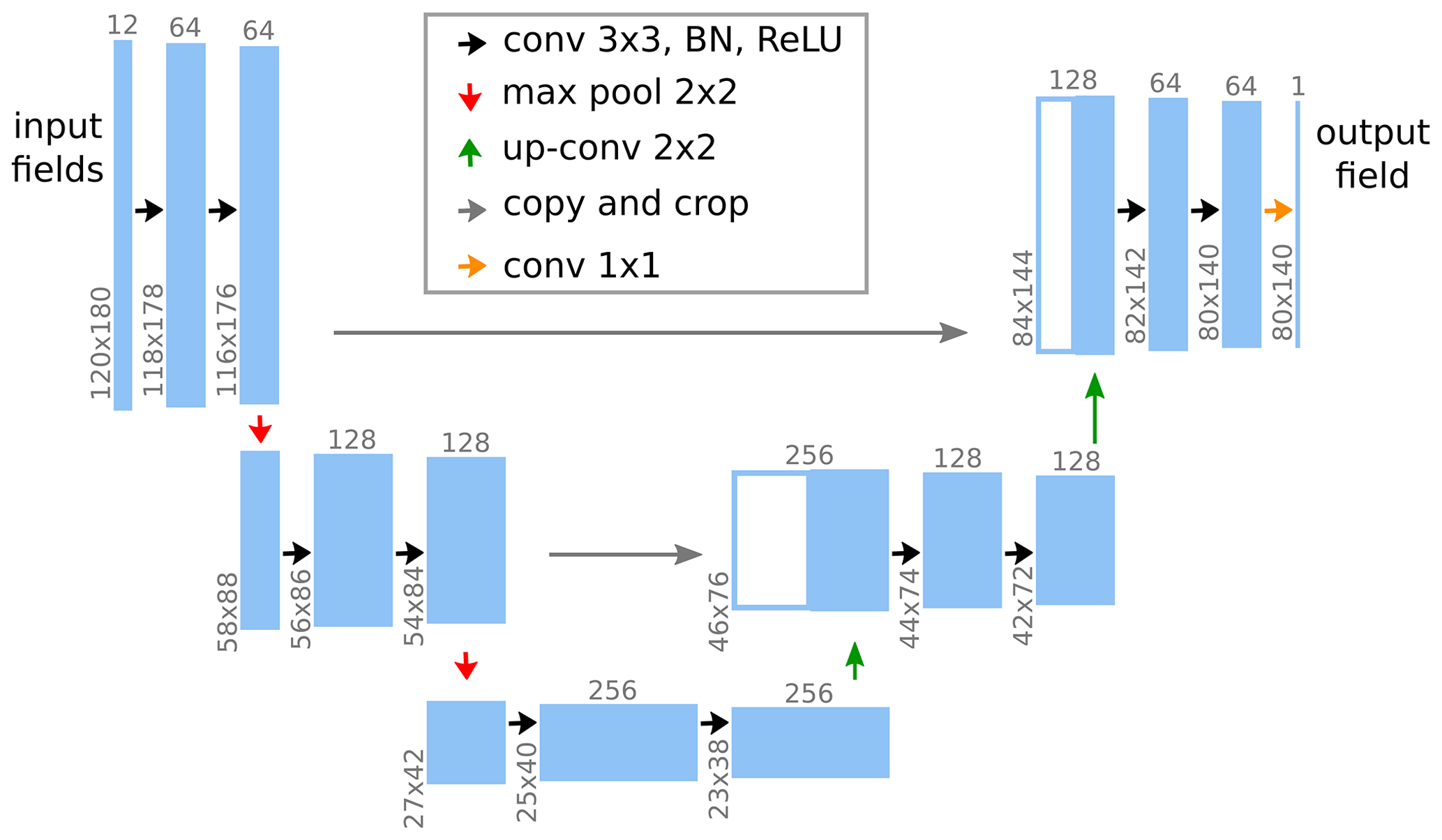
Figure 4 Model architecture in the example of soil-moisture–precipitation coupling. The leftmost blue box represents the input to the model, which consists of 12 variables (including soil moisture) at the 120×180 input pixels (see Fig. 3). This input is passed through multiple sequential modules represented by the arrows. Each module performs simple mathematical operations on its respective inputs and produces an output that is fed to the next module. This output is represented by the next blue box and, in general, differs in shape from the input, as indicated by the grey upright and rotated numbers. For details on the mathematical operations we refer to Ronneberger et al. (2015). The rightmost blue box represents the output of the model, which consists of the precipitation prediction at the 80×140 target pixels. The combination of multiple simple modules allows the model to represent complex functions.

The second concept is that of translation invariance. Translation invariance means that the function $\widehat{f}$, which maps the input variables in the receptive field to a prediction, is identical for all target locations. In our case, due to the arithmetic details of the considered model architecture (Dumoulin and Visin, 2016), the DL model is block translation invariant; i.e., the prediction at a target location (i,j) is not determined by a single function $\widehat{f}$ for all target locations but by one of 4×4 fixed functions ${\widehat{f}}_{nk},n,k=\mathrm{1},\mathrm{\dots },\mathrm{4}$, depending on the values imod4 and jmod4.

Both concepts, receptive field and translation invariance, are important features of CNNs, because they counteract overfitting, i.e., making (nearly) perfect predictions on the training data but not generalizing to unseen data. However, both concepts constitute constraints that may prevent CNNs from representing the function from Eq. (10). Indeed, the translation invariance requires including additional input variables $\mathit{\{}{C}_{\mathrm{\ell }}{\mathit{\}}}_{\mathrm{\ell }=\mathrm{1}}^k$ that lead to spatial variability in soil-moisture–precipitation coupling. We will discuss this in Sect. 3.3. Note that we can mostly ignore the general constraint of receptive fields, because the lead time of the predictions is only 4 h and the receptive field is large enough to take into account all relations between soil moisture and precipitation at that timescale.

Before training the model, we split our data into training, validation and test sets. Due to potential correlations between subsequent time steps, an entirely random split would lead to high correlations between samples in training, validation and test sets. To achieve independence between samples belonging to different sets, we randomly choose all samples from the years 2010 and 2016 for validation, all samples from the years 2012 and 2018 for testing, and all samples from the remaining 37 years for training. The test set is not used during the entire training and tuning process of the model.

During training, the Adam optimizer (Kingma and Ba, 2017) is used to adapt the approximately 2.3 million, randomly initialized weights of the model to minimize the mean squared error on the training set. In terms of implementation, we use the PyTorch (Paszke et al., 2019) wrapper skorch (Tietz et al., 2017) with default parameters for training the model: set the maximum number of epochs to 200, the learning rate in the Adam optimizer to $\mathrm{1}\times {\mathrm{10}}^{-\mathrm{3}}$, the batch size to 64, and patience for early stopping (i.e., the number of epochs after which training stops if the loss function evaluated on the validation set does not improve by some threshold) to 30 epochs. During training, we further use data augmentation. Namely, we randomly rotate by 180^∘ (or not) and subsequently horizontally flip (or not) the considered region for each training sample and each training epoch independently. Similar to the translation invariance of the model, this requires including input variables which lead to spatial variability in soil-moisture–precipitation coupling as discussed in the next section.

3.3 Choice of input variables

The choice of additional input variables $\mathit{\{}{\mathit{C}}_{\mathrm{\ell }}{\mathit{\}}}_{\mathrm{\ell }=\mathrm{1}}^k$ represents a crucial aspect of the proposed methodology for two reasons (see Sect. 2.2.2). First, we need the additional input variables to (approximately) fulfill the adjustment criteria from Sect. 2.1.2, such that the mapping of input variables $\left(\mathit{S}\mathit{M}\right[t],\mathit{\{}{\mathit{C}}_{\mathrm{\ell }}\left[t\right]{\mathit{\}}}_{\mathrm{\ell }=\mathrm{1}}^k)$ to $\mathbb{E}\left[\mathit{P}\right[t+\mathrm{4}\mathrm{h}\left]\right|\mathit{S}\mathit{M}\left[t\right],\mathit{\left\{}{\mathit{C}}_{\mathrm{\ell }}\right[t\left]{\mathit{\}}}_{\mathrm{\ell }=\mathrm{1}}^k\right]$ (see Eq. 10) is a good approximation of the map

$$\begin{array}{}\text{(12)}& \left(\mathit{S}\mathit{M}\right[t],\mathit{\{}{\mathit{C}}_{\mathrm{\ell }}\left[t\right]{\mathit{\}}}_{\mathrm{\ell }=\mathrm{1}}^k)\to \mathbb{E}[\mathit{P}[t+\mathrm{4}\mathrm{h}]\left|\mathrm{do}\right(\mathit{S}\mathit{M}\left[t\right]),\mathit{\{}{\mathit{C}}_{\mathrm{\ell }}\left[t\right]{\mathit{\}}}_{\mathrm{\ell }=\mathrm{1}}^k].\end{array}$$

Second, the choice of additional input variables affects how accurately the CNN approximates the map from Eq. (10) and finally the partial derivatives of this map with respect to SM[t] values that are computed in the sensitivity analysis (see Sect. 3.4).

Choosing additional input variables that fulfill the adjustment criteria is usually based on a causal graph of the considered system. However, a generally applicable causal graph of the Earth system does not exist. Thus, we make use of the fact that causal parents of SM[t] always fulfill the adjustment criteria; i.e., we look for a set of Earth system variables that is sufficient to determine SM[t] while not being affected by SM[t]. Given the temporal resolution of the ERA5 data and the timescale of our analysis, a reasonable example is the set of variables in the second column in Fig. 5.

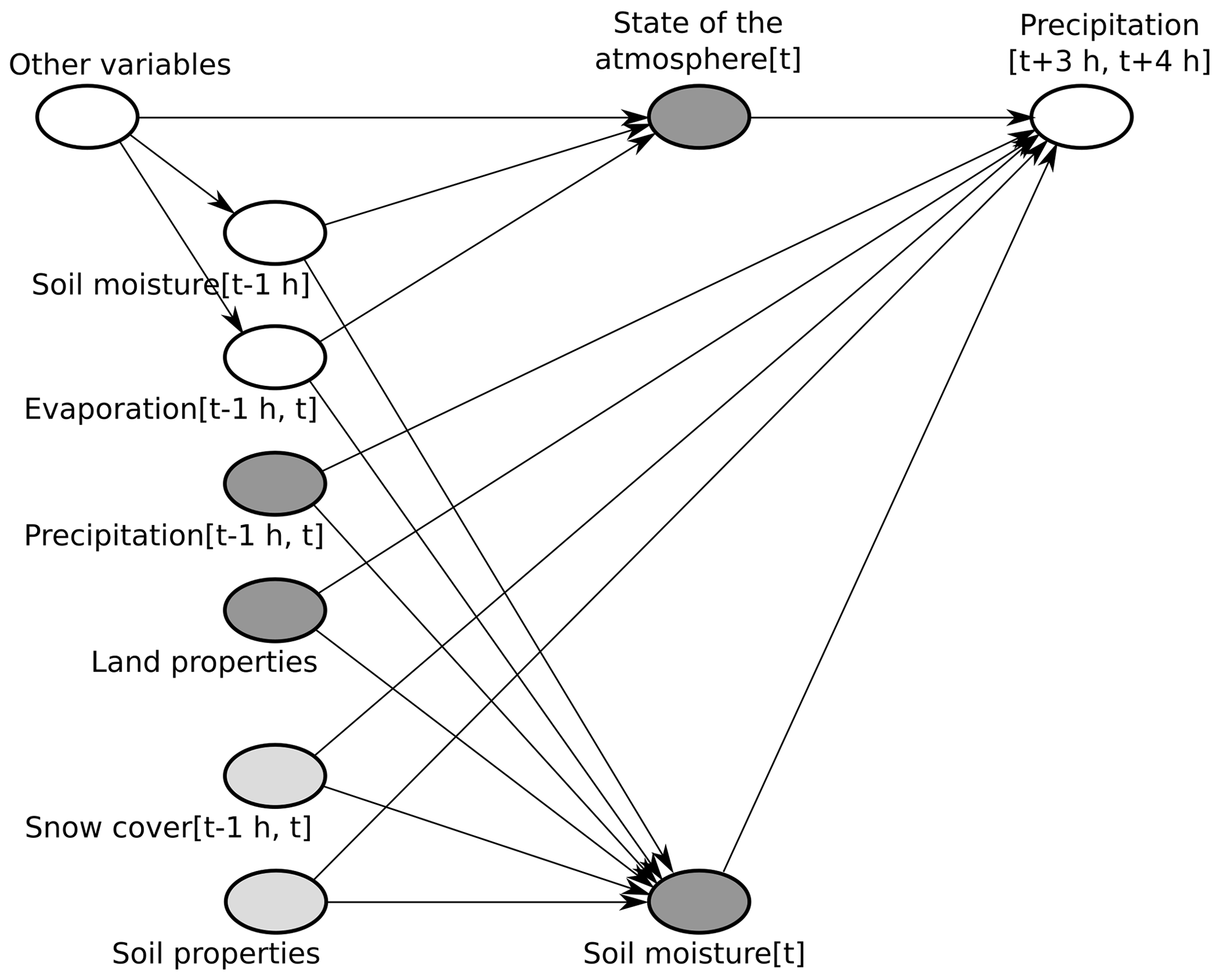
Figure 5 Causal graph in the example of soil-moisture–precipitation coupling. The dark grey nodes represent the chosen input variables, while light grey nodes represent variables that are ignored in our analysis (see text). Land properties comprise the time-independent variables topography, land–sea mask, and fractions of high and low vegetation cover. The state of the atmosphere at time t is represented by temperature and dew point temperature at 2 m height at time t, as well as wind at 100 m height at time t. In addition to these variables, we included short- and long-wave radiation at the land surface at time t. Note that the depicted causal graph only includes nodes and edges that are relevant for the adjustment criteria from Sect. 2.1.2 (e.g., no edge from “other variables” to $\mathit{P}[t-\mathrm{1}\mathrm{h},t]$, and no nodes on the causal path from SM[t] to $\mathit{P}[t+\mathrm{3}\mathrm{h},t+\mathrm{4}\mathrm{h}]$, such as evaporation $[t,t+\mathrm{3}\mathrm{h}]$).

If we included all of these variables, the adjustment criteria would be met and the map from Eq. (10) would be identical to that from Eq. (12). Nevertheless, obtaining a good approximation of the map from Eq. (10) with our DL model would be difficult due to the strong correlation between SM[t−1 h] and SM[t]. Furthermore, the strong correlation between evaporation $[t-\mathrm{1}\mathrm{h},t]$ and evaporation $[t,t+\mathrm{3}\mathrm{h}]$ may prevent us from identifying any causal effect of SM[t] on P[t+4 h], because evaporation $[t,t+\mathrm{3}\mathrm{h}]$ is a direct descendant of SM[t] on every causal path from SM[t] to P[t+4 h] (see motivation of the second adjustment criterion in Sect. 2.1.2). Therefore, we decided to exclude SM[t−1 h] and evaporation $[t-\mathrm{1}\mathrm{h},t]$. Nevertheless, this leads to unblocked non-causal paths between SM[t] and P[t+4 h] via these variables (e.g., $\mathit{S}\mathit{M}\left[t\right]\leftarrow \mathit{S}\mathit{M}[t-\mathrm{1}\mathrm{h}]\to \text{state of the atmosphere}\left[t\right]\to \mathit{P}[t+\mathrm{4}\mathrm{h}]$). To block these paths, we include additional input variables that represent the state of the atmosphere at time t.

Approximating the map from Eq. (10) and its partial derivatives with respect to SM[t] gets more difficult with increasing number of input variables. This is because additional input variables increase the complexity of this map and the general risk of overfitting. Therefore, and because SM[t−1 h] and evaporation $[t,t-\mathrm{1}\mathrm{h}]$ presumably affect the lower atmosphere more strongly than the higher atmosphere, we focus on variables representing the state of the lower atmosphere in this example.

The above considerations are valid for any model architecture and training procedure. In our example, we further must take into account the translation invariance of the considered DL model and the rotation and flipping of the region used for data augmentation during the training procedure. A seemingly valid option is to include latitude–longitude information as additional input variables. However, if we did so, the DL model would have to learn a different mapping for each location (i,j), and data augmentation in the form of flipping and rotation of the region would not be useful. Instead, we include short- and long-wave radiation at the land surface [t]. Thus, the above requirement is approximately fulfilled, and the model does not have to learn a different mapping for each location, which presumably leads to it learning a better approximation of the map from Eq. (10).

The choice of input variables is where we insert prior knowledge in the proposed methodology (see Sect. 2.2.1). There is no unique choice of input variables, but several subjective decisions that have to be made. For example, above we could have started from a different set of causal parents, e.g., going not one but several hours into the past from time t, but at least theoretically that makes no difference (see Sect. 4). Starting from a set of causal parents and replacing variables strongly correlated with X, as described above, seems to be a valid strategy for the choice of input variables, which is applicable to many relations in the Earth system besides soil-moisture–precipitation coupling. It is in line with the fact that causal parents always fulfill the adjustment criteria and with the general finding from causality research that input variables strongly correlated with X reduce the efficiency of statistical estimators of causal effects (Witte et al., 2020). The causal graph clearly conveys to other scientists the assumptions underlying a specific application of the proposed methodology.

3.4 Sensitivity analysis

Given our trained DL model, we consider different combinations of partial derivatives of the model to study the local and regional effects of soil moisture changes on precipitation (see Sect. 2.2.2). We define the causal effect of a soil moisture change at a pixel (i,j) on precipitation at the very same pixel as the local effect or local soil-moisture–precipitation coupling. Accordingly, we consider for each pixel (i,j) in the target region the partial derivative

$$\begin{array}{}\text{(13)}& q_{ij}^{\mathrm{loc}}={\displaystyle \frac{\partial {\mathit{p}}_{ij}(\mathit{S}\mathit{M},\mathit{\{}{\mathit{C}}_{\mathrm{\ell }}{\mathit{\}}}_{\mathrm{\ell }=\mathrm{1}}^k)}{\partial \mathit{S}{\mathit{M}}_{ij}}},\end{array}$$

where p_ij denotes the precipitation prediction of the DL model for pixel (i,j), and SM and $\mathit{\{}{\mathit{C}}_{\mathrm{\ell }}{\mathit{\}}}_{\mathrm{\ell }=\mathrm{1}}^k$ are the input variables to the model. We average these derivatives over all input samples $(\mathit{S}\mathit{M},\mathit{\{}{\mathit{C}}_{\mathrm{\ell }}{\mathit{\}}}_{\mathrm{\ell }=\mathrm{1}}^k)$ from the test set denoted by ${\stackrel{\mathrm{‾}}{q^{\mathrm{loc}}}}_{ij}$.

Next to the local soil-moisture–precipitation coupling, we define the regional effect or regional soil-moisture–precipitation coupling as the causal effect of a soil moisture change at a pixel (i,j) on precipitation in the entire target region. Accordingly, we consider for each pixel (i,j) in the target region the sum of partial derivatives

$$\begin{array}{}\text{(14)}& q_{ij}^{\mathrm{reg}}=\sum _{\widehat{i}=\mathrm{1}}^{\mathrm{80}}\sum _{\widehat{j}=\mathrm{1}}^{\mathrm{140}}{\displaystyle \frac{\partial {\mathit{p}}_{\widehat{i}\widehat{j}}(\mathit{S}\mathit{M},\mathit{\{}{\mathit{C}}_{\mathrm{\ell }}{\mathit{\}}}_{\mathrm{\ell }=\mathrm{1}}^k)}{\partial \mathit{S}{\mathit{M}}_{ij}}}.\end{array}$$

Note that most of the derivatives in the sum are zero, because, e.g., a change in soil moisture in Great Britain at time t does not affect precipitation in Italy 4 h later. Outside of a 52×52 pixel surrounding region, this is enforced by the architecture of the DL model (see Sect. 3.2), and inside of this region, it is learned during training of the model. As for local soil-moisture–precipitation coupling, ${\stackrel{\mathrm{‾}}{q^{\mathrm{reg}}}}_{ij}$ denotes the average of $q_{ij}^{\mathrm{reg}}$ over all input samples from the test set.

To obtain robust results, we computed local and regional couplings for 10 instances of the DL model that were trained from different random weight initializations. Next, we averaged the obtained couplings (${\stackrel{\mathrm{‾}}{q^{\mathrm{loc}}}}_{ij}$ and ${\stackrel{\mathrm{‾}}{q^{\mathrm{reg}}}}_{ij}$) over the 10 instances. The results are shown in Fig. 6. Notably, the difference in sign between positive local and negative regional impact demonstrates the importance of taking into account non-local effects of soil-moisture–precipitation coupling, which are neglected by many other approaches. Moreover, Fig. 6 indicates particularly strong local and regional couplings in mountainous regions and ridges. We will further discuss the correctness of these results in Sect. 4.

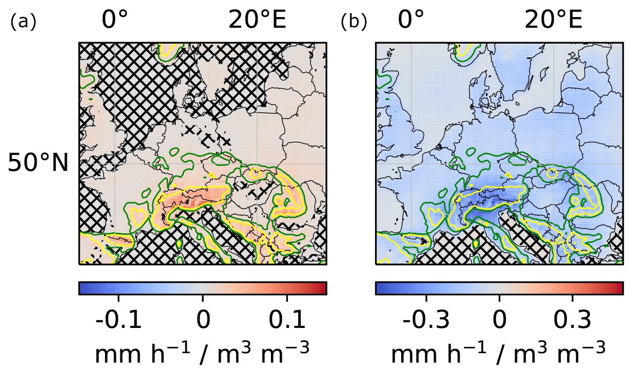
Figure 6 Local and regional soil-moisture–precipitation couplings. (a) Impact of local soil moisture changes (m³ water m⁻³ soil) on local precipitation (mm h⁻¹) for each pixel in the target region (in the text denoted by ${\stackrel{\mathrm{‾}}{q^{\mathrm{loc}}}}_{ij}$). (b) Impact of local soil moisture changes on regional precipitation for each pixel in the target region (in the text denoted by ${\stackrel{\mathrm{‾}}{q^{\mathrm{reg}}}}_{ij}$). For better comparability of local and regional values, the unit mm h⁻¹ for precipitation refers to a single pixel in both panels. Missing hatching indicates that the coupling reflects more than random correlations between soil moisture and precipitation in the training data, artifacts of the DL training procedure, seasonality, and the correlation between soil moisture and topography (see Sect. 4.2). The green and yellow elevation contour lines indicate 370 and 750 m, respectively.

3.5 Comparison to other approaches

A common approach for studying relations in the Earth system is to consider the linear correlation between variables (Froidevaux et al., 2014; Welty and Zeng, 2018; Holgate et al., 2019). Here, we compare our results on regional soil-moisture–precipitation coupling to results obtained from a linear correlation analysis. For each location in the considered target region, Fig. 7 shows the linear correlation coefficient of soil moisture SM[t] at that location and subsequent precipitation P[t+4 h] summed over the 15×15 pixel surrounding region. In contrast to our analysis of regional soil-moisture–precipitation coupling, the linear correlation analysis assumes linearity of relations between local soil moisture and regional precipitation and neglects the difference between causality and correlation. The obtained regional soil-moisture–precipitation coupling in Fig. 7 then also differs in sign and spatial pattern from the coupling in the right panel of Fig. 6, stressing the importance of accounting for non-linear effects and for the difference between causality and correlation in the proposed methodology.

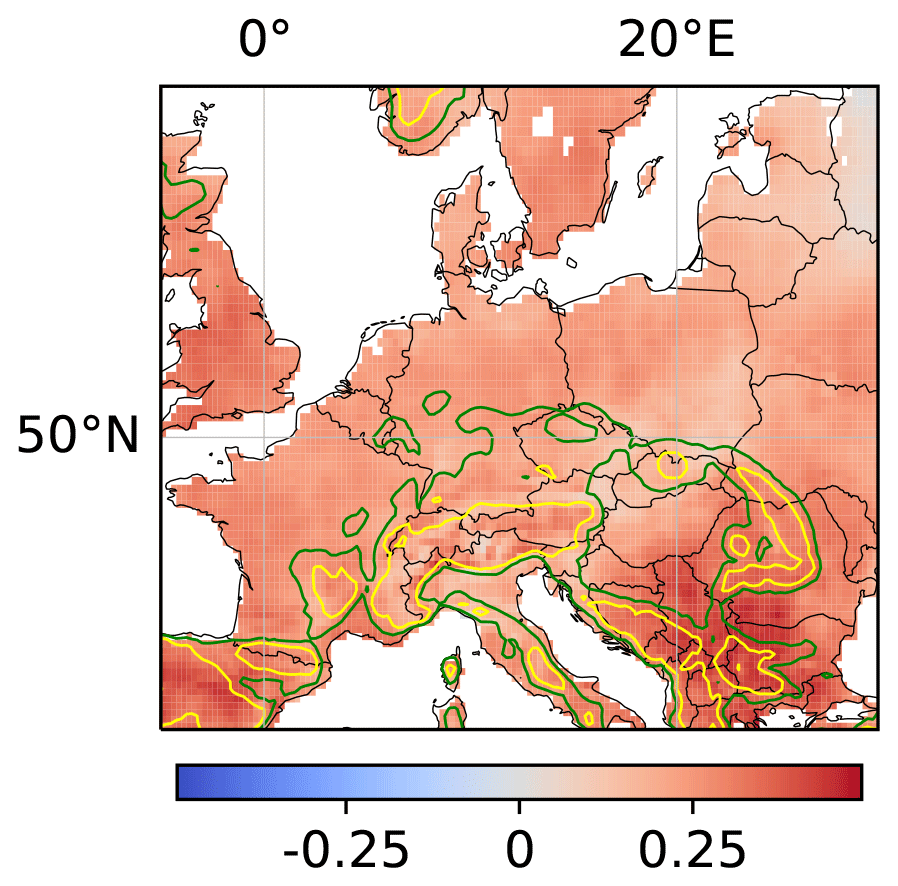
Figure 7 Linear correlation coefficient of local soil moisture and regional precipitation. For each location, the linear correlation coefficient of soil moisture SM[t] at the location and subsequent precipitation P[t+4 h] summed over the 15×15 pixel surrounding region of the location is shown.

Another approach for studying soil-moisture–precipitation coupling is to perform multiple numerical simulations that differ only in initial soil moisture and to analyze the differences in precipitation between these simulations (Imamovic et al., 2017; Baur et al., 2018; Leutwyler et al., 2021). This approach allows us to evaluate the effects of soil moisture changes on precipitation within the employed numerical model precisely. However, for some questions, it is computationally infeasible. For instance, in this work, we used ERA5 data to analyze the effects of soil moisture changes at each of 80×140 target pixels on subsequent precipitation in the target region. We averaged these effects over all time steps in 2 test years, constituting 2208 time steps. Performing an analogous study based on numerical simulations would require at least $\mathrm{80}\times \mathrm{140}\times \mathrm{2208}=\mathrm{24}\mathrm{729}\mathrm{600}$ 4-hourly simulations with the ECMWF Earth system model used to produce the considered ERA5 data. Each simulation would be initialized with the state of the reference simulation at one of the 2208 considered time steps, with the only difference being that soil moisture would be slightly increased or decreased at one of the 80×140 target pixels. This corresponds to simulating more than 10 000 years with the ECMWF Earth system model and is computationally infeasible. Furthermore, an advantage of the proposed methodology over approaches based on numerical simulations is that it can directly be applied to observational data, if suitable observational data are available. In this case, the proposed methodology does not rely on any assumptions incorporated into numerical models.

4 Additional analyses to verify the results

To ensure that the proposed methodology provides reliable results, this section presents some additional analyses. Theoretically, the proposed methodology determines the causal effect of X on Y exactly. However, in practice, we make two important approximations (see Sect. 2.2.2). First, the additional input variables $\mathit{\{}{\mathit{C}}_{\mathrm{\ell }}{\mathit{\}}}_{\mathrm{\ell }=\mathrm{1}}^k$ may not strictly fulfill the adjustment criteria from Sect. 2.1.2, such that the mapping of input variables to the original expected value $\mathbb{E}\left[\mathit{Y}\right|\mathit{X}=\mathit{x},\mathit{\{}{\mathit{C}}_{\mathrm{\ell }}={\mathit{c}}_{\mathrm{\ell }}{\mathit{\}}}_{\mathrm{\ell }=\mathrm{1}}^k]$ in Eq. (6) is only approximately identical to the mapping to the post-intervention expected value $\mathbb{E}\left[\mathit{Y}\right|\mathrm{do}(\mathit{X}=\mathit{x}),\mathit{\{}{\mathit{C}}_{\mathrm{\ell }}={\mathit{c}}_{\mathrm{\ell }}{\mathit{\}}}_{\mathrm{\ell }=\mathrm{1}}^k]$ in Eq. (5). Second, the DL model represents only an approximation of the map from Eq. (6). Both errors are difficult to quantify, because both maps are unknown.

For example, the performance of the DL model on the test set cannot indicate how well the DL model approximates the map from Eq. (6), because the loss value for this map is not known. For instance, for a system described by the causal graph $\mathit{X}\to \mathit{Y}\leftarrow \mathit{C}$ and the structural equation $\mathit{Y}=\mathit{X}+\mathrm{1000}\cdot \mathit{C}$ (where X and C vary in similar ranges), the adjustment criteria from Sect. 2.1.2 imply that it suffices to consider X as the only input variable in the proposed methodology. Nevertheless, even if the trained DL model perfectly represented the map $\mathit{x}\to \mathbb{E}\left[\mathit{Y}\right|\mathit{X}=\mathit{x}]$, the associated loss value would be high as knowing X does not reveal much about Y, which is mainly determined by C.

The results of the proposed methodology are the partial derivatives $\stackrel{\mathrm{‾}}{q_{ij}}$ of the DL model computed in the sensitivity analysis. Due to the above approximations, these derivatives are only approximations of the partial derivatives $\stackrel{\mathrm{‾}}{s_{ij}}$ of the map from Eq. (5), which represent the causal effect of X on Y (see Sect. 2.2.2). However, even quantifying the two approximation errors mentioned above would not give us a good estimate of the errors in these results. In this section, we propose several additional analyses to build confidence in results obtained with the proposed methodology. Particularly, the proposed analyses show if results are statistically significant, i.e., reflect more than random correlations or artifacts of the DL training procedure (Sect. 4.1), and if they reflect more than specific (known) correlations (Sect. 4.2). Moreover, the analyses proposed in Sect. 4.3 allow us to identify (potentially unknown) spurious correlations in the results. Finally, we propose some further sanity checks in Sect. 4.4. We illustrate the analyses with our results on soil-moisture–precipitation coupling from Sect. 3.

For reference only, we provide here the normalized mean squared error on the test set (target variable normalized to a mean of 0 and standard deviation of 1 on the training set) for our application to soil-moisture–precipitation coupling: it is 0.60 for the DL model. For a persistence prediction, i.e., when predicting the input P[t] as target P[t+4 h], which is a simple baseline prediction, it is 1.54.

4.1 Statistical significance

To test whether results obtained with the proposed methodology are statistically significant, i.e., represent more than random correlations between X and Y in the training data and random artifacts of the procedure for training the DL model, we propose the following procedure. First, randomly permute X in the training data, thereby breaking all non-random correlations between X and Y. For example, in the application to soil-moisture–precipitation coupling, permute soil moisture temporally and spatially. Next, train a separate instance of the original DL model with a random initialization of model weights on the modified training data. Repeat this procedure several times. If the original results deviate significantly from the results obtained from this procedure, they are statistically significant.

Formally, we propose to interpret a result r∈ℝ of the proposed methodology, e.g., local or regional soil-moisture–precipitation coupling at some pixel (i,j) (see Sect. 3.4), as a sample of a random variable $\widehat{r}:\mathrm{\Omega }\to \mathbb{R}$, where Ω is the probability space

$$\begin{array}{}\text{(15)}& \mathrm{\Omega }=\mathit{\left\{}\text{Training data}\mathit{\right\}}\times \mathit{\left\{}\text{Weight initialization of the DL model}\mathit{\right\}}.\end{array}$$

Thus, $\widehat{r}$ computes the considered result, e.g., local or regional soil-moisture–precipitation coupling at pixel (i,j) according to the proposed methodology, for any given sample ω∈Ω. We define the null hypothesis that r represents random correlations between X and Y in the training data or random artifacts of the procedure for training the DL model. To test this hypothesis, we create m samples ${\mathit{\omega }}_{\mathrm{0}}^{\mathrm{1}},\mathrm{\dots },{\mathit{\omega }}_{\mathrm{0}}^m$ of Ω by the above-described procedure of permuting X and randomly initializing the weights of separate instances of the considered DL model. Moreover, we compute the associated values $r_{\mathrm{0}}^i=\widehat{r}\left({\mathit{\omega }}_{\mathrm{0}}^i\right),i=\mathrm{1},\mathrm{\dots },m$, representing samples of $\widehat{r}$ under the null hypothesis.

If the original value r differs from these samples, we can reject the null hypothesis and conclude that r is statistically significant. In particular, if m is large enough, we can reject the null hypothesis at some significance level α (e.g., α=5 %), if the original value r lies outside the middle 100 %−α of the values $r_{\mathrm{0}}^{\mathrm{1}},\mathrm{\dots },r_{\mathrm{0}}^m$, i.e., if

$$\begin{array}{}\text{(16)}& \begin{array}{rl}& r\notin \left[\text{percentile}\right(\mathit{\{}{r}_{\mathrm{0}}^{\mathrm{1}},\mathrm{\dots },r_{\mathrm{0}}^m\mathit{\}},\mathit{\alpha }/\mathrm{2}),\\ & \text{percentile}\left(\mathit{\right\{}{r}_{\mathrm{0}}^{\mathrm{1}},\mathrm{\dots },r_{\mathrm{0}}^m\mathit{\}},\mathrm{100}\mathit{\%}-\mathit{\alpha }/\mathrm{2})].\end{array}\end{array}$$

However, because we have to train m DL models for this analysis, it may not be feasible to choose m large enough to get reasonable approximations of these percentiles. In this case, we propose computing the mean μ and standard deviation σ of the values $r_{\mathrm{0}}^{\mathrm{1}},\mathrm{\dots },r_{\mathrm{0}}^m$, assuming a normal distribution of $\widehat{r}$ under the null hypothesis, and rejecting the null hypothesis at significance level α if r is not in the middle 100 %−α of the distribution N(μ,σ), i.e., if

$$\begin{array}{}\text{(17)}& \begin{array}{rl}& r\notin \left[\text{percentile}\right(N(\mathit{\mu },\mathit{\sigma }),\mathit{\alpha }/\mathrm{2}),\text{percentile}(N(\mathit{\mu },\mathit{\sigma }),\\ & \mathrm{100}\mathit{\%}-\mathit{\alpha }/\mathrm{2}\left)\right].\end{array}\end{array}$$

4.2 Known spurious correlations

As mentioned above, the proposed methodology identifies the exact causal effect of X on Y in theory, but not necessarily in practice, where results might reflect spurious correlations. In this section, we propose two analyses to test whether results obtained with the proposed methodology represent more than spurious correlations. The analyses apply whenever the spurious correlations are known, and X can be permuted such that the considered correlations are preserved while other correlations between X and Y break. For example, there exists a spurious correlation between SM[t] and P[t+4 h] via topography, because topography affects both SM[t] and P[t+4 h] ($\mathit{S}\mathit{M}\left[t\right]\leftarrow \text{topography}\to \mathit{P}[t+\mathrm{4}\mathrm{h}]$; see Sect. 2.1.1). Further, there might exist a spurious correlation between SM[t] and P[t+4 h] via seasonality, e.g., if both soil moisture and precipitation were generally lower in August than in June. Both correlations are preserved if we permute soil moisture year-wise as illustrated in Fig. 8. All other cases of spurious correlations are discussed in the next section, in particular unknown spurious correlations.

Figure 8 Modification of the training data for the year-wise permutation of SM[t]. The modification of the test data works analogously.

The first proposed analysis is identical to the analysis described in Sect. 4.1 except that X in the training data is not permuted randomly but in such a way that the considered spurious correlations are preserved. If the original results deviate significantly from the results obtained in this analysis, they are statistically significant and do not only represent the considered spurious correlations. In our example of soil-moisture–precipitation coupling, we permuted SM[t] year-wise as illustrated in Fig. 8 and trained m=10 separate instances of the DL model. The analysis indicates that our results on soil-moisture–precipitation coupling are statistically significant and represent more than correlations between soil moisture and topography or seasonality (missing hatching in Fig. 6). Intriguingly, the regional coupling is statistically significant (albeit weak) at most ocean locations, although one would not expect the DL model to learn a systematic effect of soil moisture variations on precipitation at these locations, since soil moisture does not vary at these locations. Indeed, we set soil moisture to 1 m³ water per cubic meter at all ocean locations for all time steps, while it is smaller than 0.75 at all non-ocean locations. We assume that the statistical significance of the regional coupling at ocean locations is an artifact of the DL model architecture, which favors generalization between locations, ocean and non-ocean.

The second proposed analysis evaluates whether the original DL model learned useful information in terms of predictive performance on the relation between X and Y, apart from the considered spurious correlations. In the analysis, we train m separate instances of the original DL model on the original training data. The m instances differ in the random initialization of model weights (see Sect. 3.4). For each model instance, we compute the value of the loss function on the test set, obtaining m values $l_{\mathrm{1}},\mathrm{\dots },l_m\in \mathbb{R}$. Next, for each model instance separately, we randomly permute X in the test data such that the considered spurious correlations are preserved, and we compute the value of the loss function on the modified test set, obtaining m values $l_{\mathrm{1}}^{\text{perm}},\mathrm{\dots },l_m^{\text{perm}}\in \mathbb{R}$. Finally, we use a permutation test (Hesterberg, 2014) to test if the expected value of the loss function is smaller on the original test set than on the modified test set. If this is the case, the DL models learned something useful in terms of predictive performance on the relation between X and Y, apart from the considered spurious correlations. In our example of soil-moisture–precipitation coupling, we trained m=10 separate instances of the DL model. We considered the year-wise permutation of soil moisture in the test data as described above. In this case, the analysis indicates at a confidence level of 99 % that the model learned useful information in terms of predictive performance on soil-moisture–precipitation coupling, apart from the correlations between soil moisture and topography or seasonality. However, for the validity of this analysis, it may be limiting that there are only two test years in this example and thus only one possible permutation of years apart from the original one. Therefore, we repeated the analysis and permuted soil moisture in the test data completely randomly in time. While this does not preserve correlations between soil moisture and seasonality, it still preserves the correlation between soil moisture and topography. Furthermore, it ensures the validity of the analysis as there are a lot of possible permutations. In this case, the analysis indicates at a confidence level of 99 % that the model learned useful information in terms of predictive performance on soil-moisture–precipitation coupling, apart from the correlation between soil moisture and topography. Note that even if the first analysis indicates that some result reflects more than the considered correlations, it cannot exclude that the results are partly affected by the considered spurious correlations. Analogously, if the second analysis indicates that the DL model learned useful information in terms of predictive performance on the relation between X and Y, apart from the considered spurious correlations, it cannot exclude that the predictions are partly affected by the considered spurious correlations.

4.3 Further spurious correlations

In the previous section, we analyzed specific spurious correlations, i.e., spurious correlations that were known, and for that X could be permuted such that the spurious correlations are preserved, while other correlations between X and Y break. As an additional analysis to identify any spurious correlations reflected in obtained results, we propose a variant approach. The concept of the approach is related to the ideas in Tesch et al. (2021) and Peters et al. (2016). It consists of training separate instances of the original DL model (referred to as variant models) on modified prediction tasks (referred to as variant tasks) for which it is assumed that causal relations between input and target variables either remain stable or vary in specific ways. Subsequently, the results obtained from original and variant models are compared, and it is evaluated whether they reflect the assumed stability or specific variations, respectively, of causal relations. If not, the original model or one of the variant models (or all models) learned spurious correlations.

For example, we may assume that the general (causal) mechanisms of soil-moisture–precipitation coupling do not vary in time or space. Then, if the couplings in Fig. 6 reflect the causal effect of soil moisture on precipitation, we should obtain the same couplings from separate instances of the DL model that are trained only on

• data from the first or second half of the training years;

• data from June, July or August; or

• the left or right half of the considered region.

On the other hand, if Fig. 6 reflected spurious correlations and these spurious correlations differed for the different subsets of training data listed above, we should obtain different couplings from the different model instances.

Appendix Figs. A1 to A3 show the local and regional couplings obtained from the different model instances trained on the listed training subsets. As expected for the case in which all instances learned the causal effect of soil moisture on precipitation, all couplings are very similar to the ones shown in Fig. 6. Note, however, that this does not guarantee that they show causal relations.

4.4 Task-specific sanity checks

To further assess the correctness and increase trust in results obtained from the proposed methodology, we propose to perform further, task-specific sanity checks. For instance, in our example of soil-moisture–precipitation coupling, precipitation P can be partitioned into convective precipitation P_con (occurring at spatial scales smaller than the spatial resolution of the numerical model) and large-scale precipitation P_ls (occurring at larger spatial scales), such that $\mathit{P}={\mathit{P}}_{\mathrm{con}}+{\mathit{P}}_{\mathrm{ls}}$. Accordingly, soil-moisture–precipitation coupling, SM–P coupling, can be decomposed into the sum of SM–P_con coupling and SM–P_ls coupling. As a sanity check for the results in Fig. 6, we applied the proposed methodology to obtain SM–P_con coupling and SM–P_ls coupling by replacing P by P_con and P_ls, respectively, and compared the sum of the obtained couplings with Fig. 6. Appendix Fig. A5 shows the sum of local and regional SM–P_con and SM–P_ls couplings, which are indeed very similar to the couplings shown in Fig. 6.

Further, SM–P coupling can approximately be factorized into instantaneous (local) soil-moisture–evaporation (SM–E) coupling times evaporation–precipitation (E–P) coupling. As another sanity check for the results in Fig. 6, we applied the proposed methodology to obtain SM–E coupling and E–P coupling by once replacing the target variable P by E and the other time replacing the input variable SM by E. Appendix Fig. A7 shows the product of local SM–E and local and regional E–P couplings. The obtained couplings are very similar to the couplings shown in Fig. 6, despite being slightly weaker in general and far weaker in the high Alps.

4.5 Control experiment

As a simple control experiment for the proposed methodology and analyses, we replaced the target variable P[t+4 h] by random noise. As expected from the missing correlations between SM[t] and random noise, the methodology identified no statistically significant (see Sect. 4.1) causal effect of soil moisture on the target variable in this case.

Defining a more complex control experiment confirming the results obtained in the application to soil-moisture–precipitation coupling is not possible. This is because the maps in Eqs. (6) and (5), and thus the errors in their approximations, would differ if, for example, we replaced SM[t] by a variable X that is highly correlated with P[t+4 h] but does not causally affect P[t+4 h]. However, we believe that the analyses proposed in this section build high confidence in the methodology and the results.

5 Conclusions

In this study, we proposed a novel methodology for studying complex, e.g., non-linear and non-local, relations in the Earth system. The methodology is based on the recent idea of training and analyzing a DL model to gain new scientific insights into the relations between input and target variables. It extends this idea by combining it with concepts from causality research. A crucial aspect in the proposed methodology is the choice of additional input variables for the DL model. This choice requires prior knowledge on which variables are relevant to the considered relation and on the existence of dependencies between these variables. However, it does not require prior knowledge on the strength or sign of these dependencies, which can be obtained from the proposed methodology. When the required prior knowledge does not exist, methods from causal discovery (Guo et al., 2021) might be used to identify a causal graph anyway, such that the proposed methodology might still be applicable.

In addition to the methodology, we presented analyses to assess whether results obtained with the proposed methodology are statistically significant, i.e., reflect more than random correlations or artifacts of the DL training procedure; whether they reflect more than specific (known) correlations; and whether they actually reflect causal rather than (potentially unknown) spurious correlations. Finally, we proposed sanity checks for the obtained results. While the analyses cannot guarantee the correctness of obtained results, we believe that the proposed analyses provide a solid indication of the correctness of obtained results. Taking into account the difference between causality and correlation, and overcoming common assumptions on linearity and locality in statistical approaches, as well as high computational costs and assumptions of numerical approaches, we believe that the proposed methodology may yield new scientific insights into various complex mechanisms in the Earth system.

As an illustrating example, we applied the methodology and the proposed analyses to study soil-moisture–precipitation coupling in ERA5 climate reanalysis data across Europe. Our main findings are the difference in sign between positive local and negative regional impact and particularly strong local and regional couplings in mountainous regions and ridges. While we believe that these findings may contribute to a better understanding of soil-moisture–precipitation coupling, in this article, we focused on demonstrating the methodology. An extension and discussion of our results on soil-moisture–precipitation coupling in terms of physical processes are the subject of a future study.

Appendix A

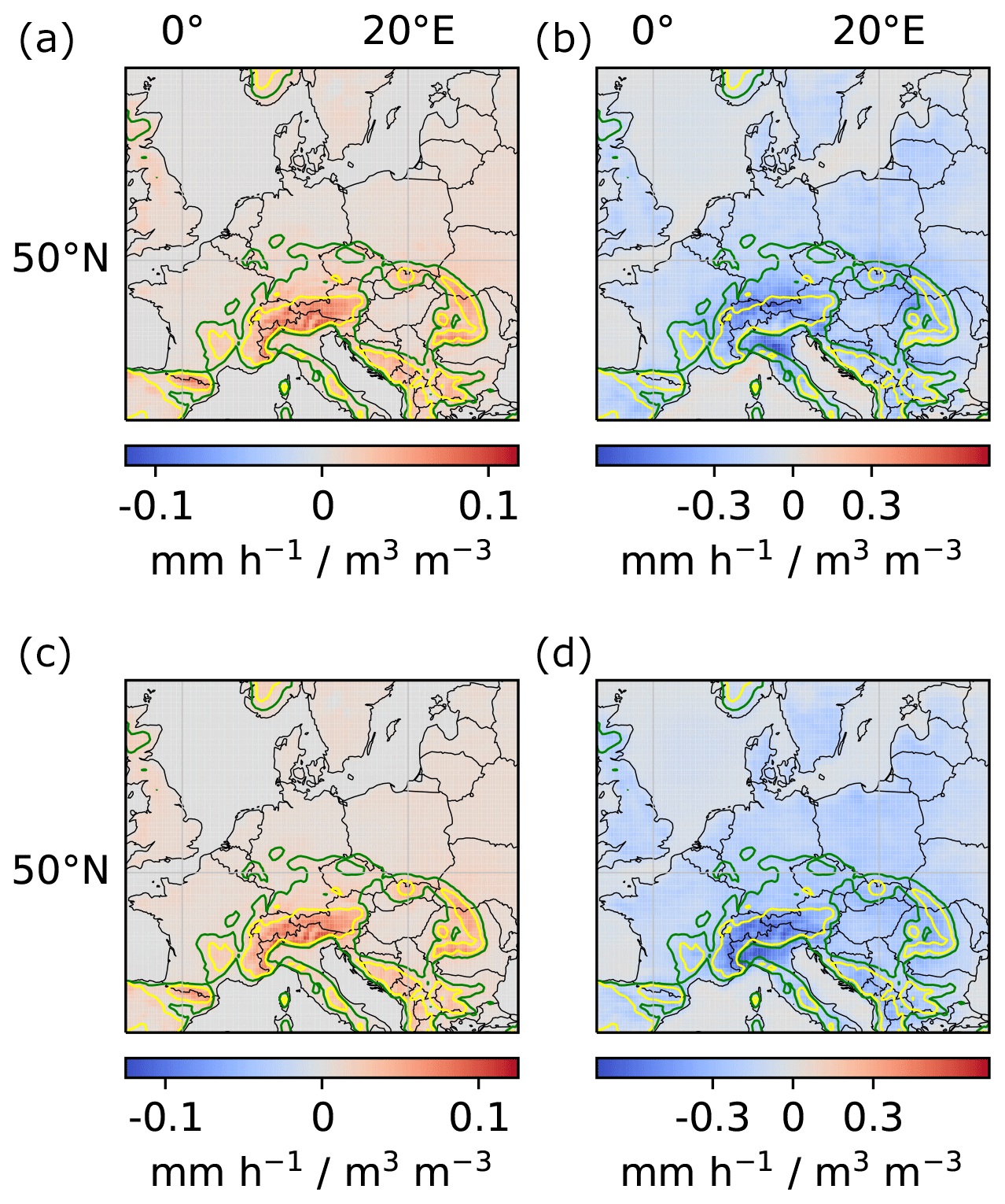
Figure A1 Local and regional soil-moisture–precipitation couplings for models trained on the first and second half of the training years, respectively. (a, c) Local couplings. (b, d) Regional couplings. (a, b) Model trained on the first half of all training years (1979–1997). (c, d) Model trained on the second half of all training years (1998–2019).

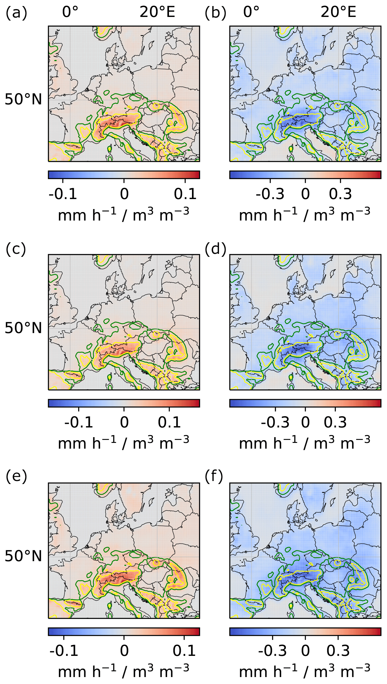
Figure A2 Local and regional soil-moisture–precipitation couplings for models trained only on data from June, July and August, respectively. (a, c, e) Local couplings. (b, d, f) Regional couplings. (a, b) Model trained on data from June. (c, d) Model trained on data from July. (e, f) Model trained on data from August.

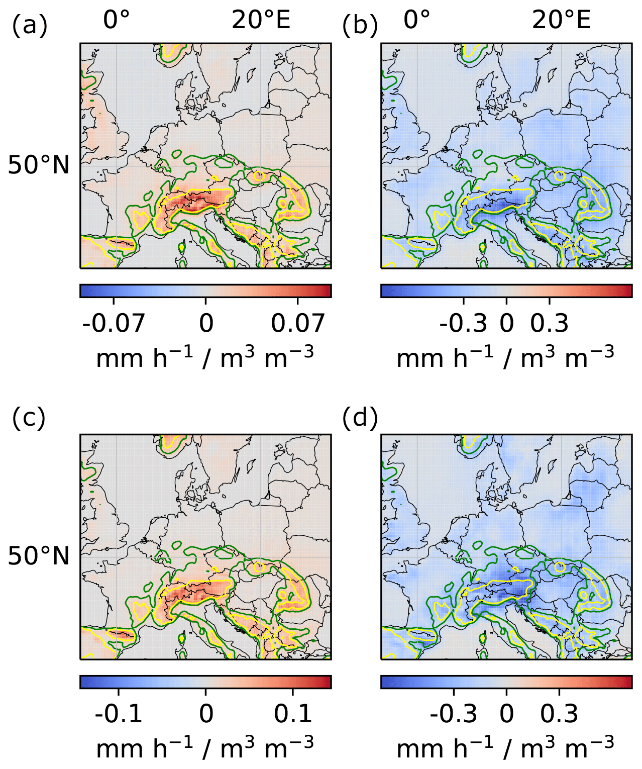
Figure A3 Local and regional soil-moisture–precipitation couplings for models trained on the left and right half of the considered region, respectively. (a, c) Local couplings. (b, d) Regional couplings. (a, b) Model trained on the left half of the considered region. (c, d) Model trained on the right half of the considered region (see Appendix Fig. A4). Note that the models were trained only on the left and right half, respectively, but the model architecture allows us to compute local and regional couplings for the entire region.

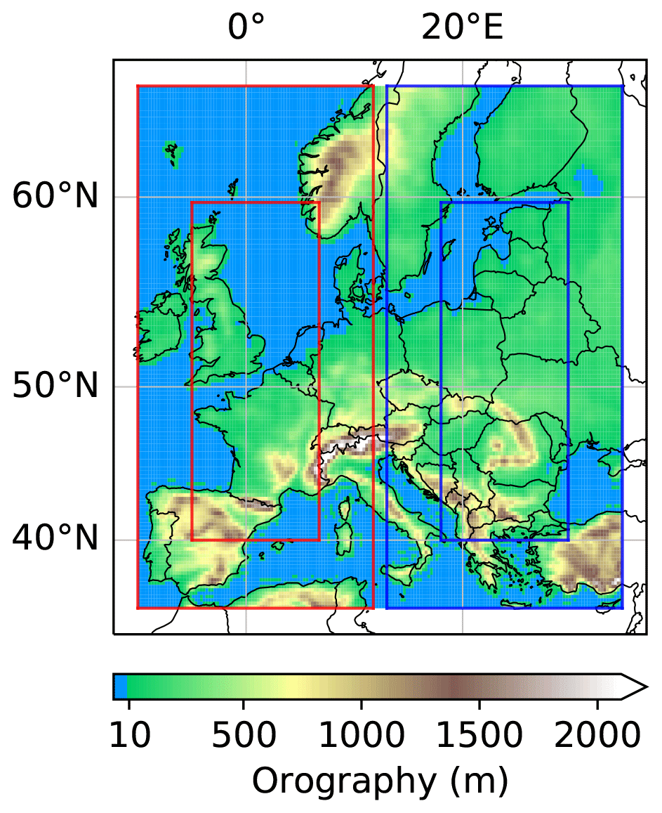
Figure A4 Location variant tasks. The input region was divided into a left and a right input region with corresponding target regions (indicated by the red and blue boxes).

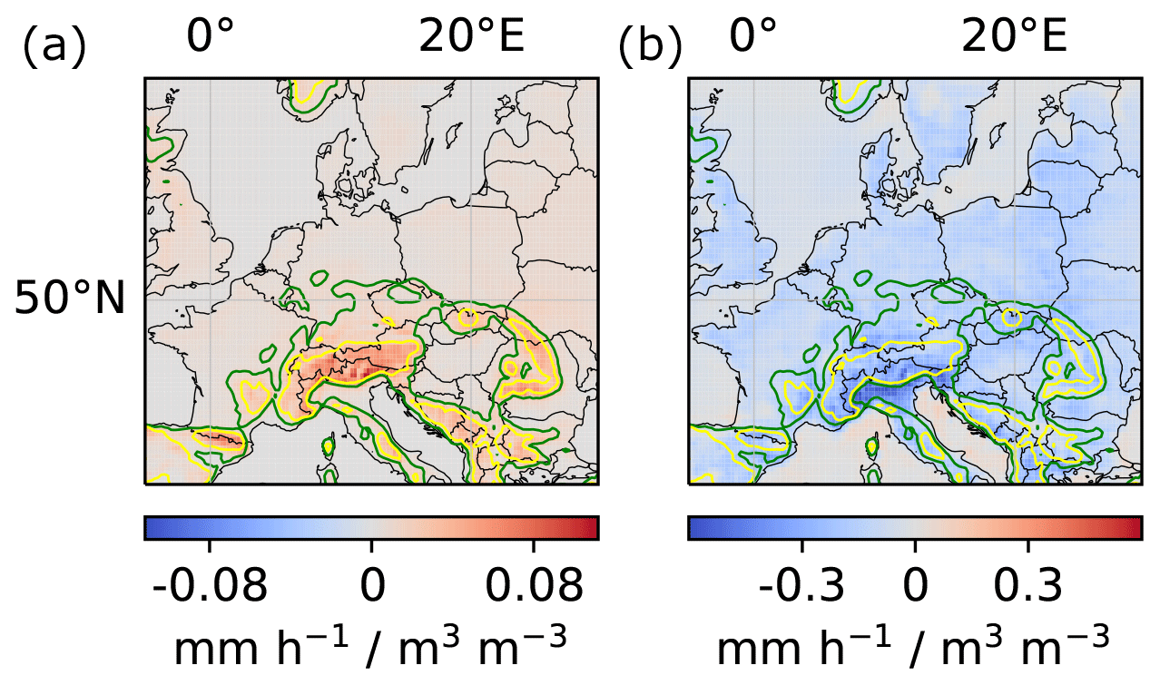
Figure A5 Sum of local and regional soil-moisture–convective-precipitation and soil-moisture–large-scale-precipitation couplings. (a) Sum of local couplings. (b) Sum of regional couplings. See Appendix Fig. A6 for soil-moisture–convective-precipitation and soil-moisture–large-scale-precipitation couplings.

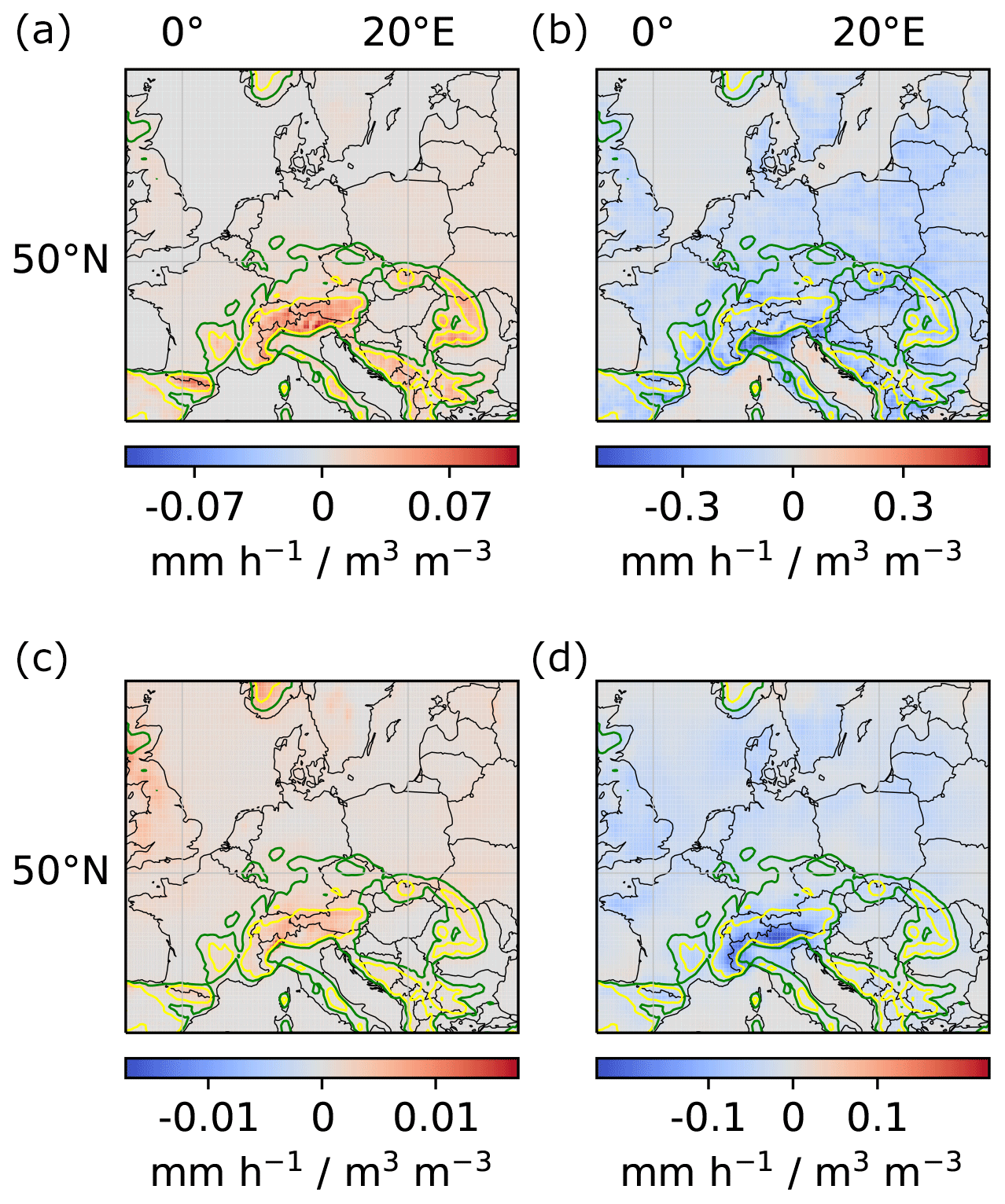
Figure A6 Local and regional soil-moisture–convective-precipitation and soil-moisture–large-scale-precipitation couplings. (a, c) Local couplings. (b, d) Regional couplings. (a, b) Soil-moisture–convective-precipitation coupling. (c, d) Soil-moisture–large-scale-precipitation coupling.

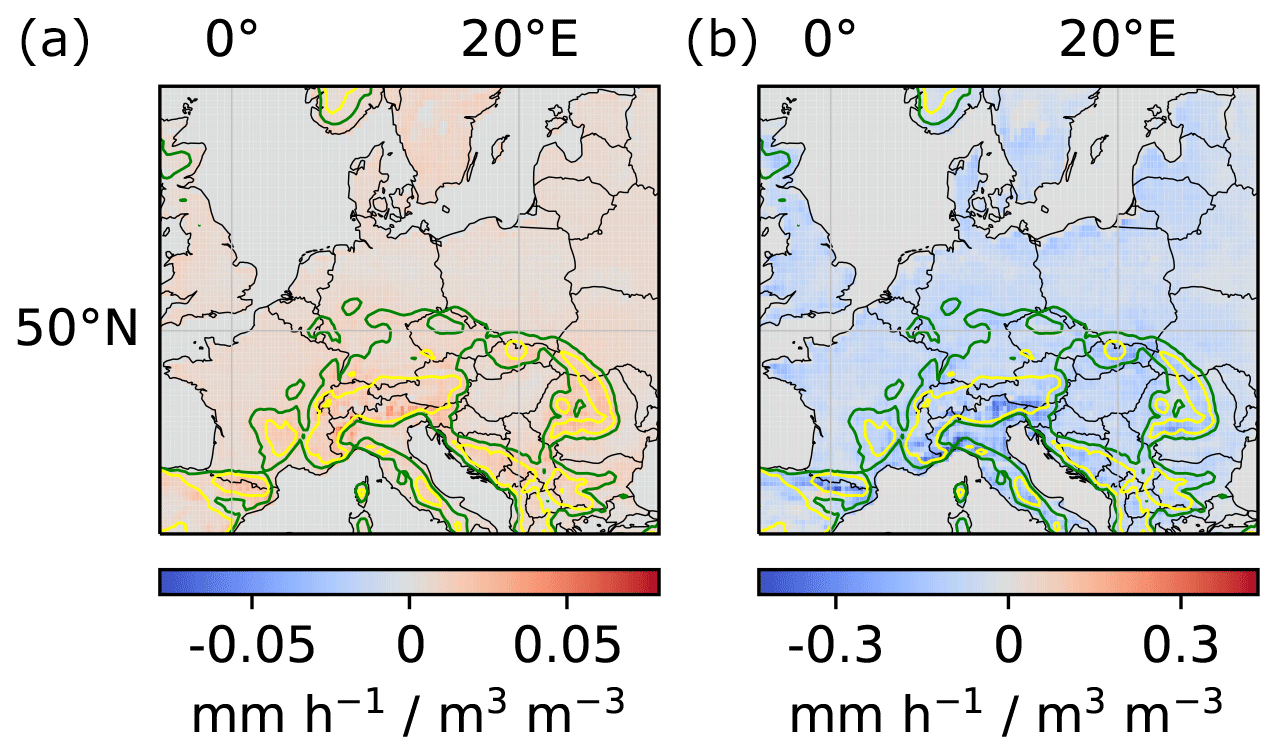
Figure A7 Product of local soil-moisture–evaporation and local and regional evaporation–precipitation couplings. (a) Product of local soil-moisture–evaporation and local evaporation–precipitation couplings. (b) Product of local soil-moisture–evaporation and regional evaporation–precipitation couplings. See Appendix Fig. A8 for local soil-moisture–evaporation and local and regional evaporation–precipitation couplings.

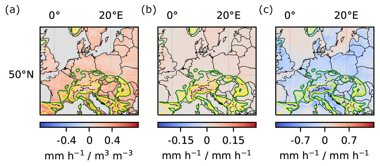
Figure A8 Local soil-moisture–evaporation and local and regional evaporation–precipitation couplings. (a) Local soil-moisture–evaporation coupling. (b) Local evaporation–precipitation coupling. (c) Regional evaporation–precipitation coupling.