Estimation of CH₄ emission based on an advanced 4D-LETKF assimilation system

Methane (CH₄) is the second major greenhouse gas after carbon dioxide (CO₂) which has substantially increased during recent decades in the atmosphere, raising serious sustainability and climate change issues. Here, we develop a data assimilation system for in situ and column-averaged concentrations using a local ensemble transform Kalman filter (LETKF) to estimate surface emissions of CH₄. The data assimilation performance is tested and optimized based on idealized settings using observation system simulation experiments (OSSEs), where a known surface emission distribution (the truth) is retrieved from synthetic observations. We tested three covariance inflation methods to avoid covariance underestimation in the emission estimates, namely fixed multiplicative (FM), relaxation-to-prior spread (RTPS), and adaptive multiplicative. First, we assimilate the synthetic observations at every grid point at the surface level. In such a case of dense observational data, the normalized root mean square error (RMSE) in the analyses over global land regions is smaller by 10 %–15 % in the case of RTPS covariance inflation method compared to FM. We have shown that integrated estimated flux seasonal cycles over 15 regions using RTPS inflation are in reasonable agreement between true and estimated flux, with 0.04 global normalized annual mean bias. We then assimilated the column-averaged CH₄ concentration by sampling the model simulations at Greenhouse Gases Observing Satellite (GOSAT) observation locations and time for another OSSE. Similar to the case of dense observational data, the RTPS covariance inflation method performs better than FM for GOSAT synthetic observation in terms of normalized RMSE (2 %–3 %) and integrated flux estimation comparison with the true flux. The annual mean averaged normalized RMSE (normalized mean bias) in LETKF CH₄ flux estimation in the case of RTPS and FM covariance inflation is found to be 0.59 (0.18) and 0.61 (0.23), respectively. The χ² test performed for GOSAT synthetic observations assimilation suggests high underestimation of background error covariance in both RTPS and FM covariance inflation methods; however, the underestimation is much higher (>100 % always) for FM compared to RTPS covariance inflation method.

1 Introduction

Methane (CH₄) is the second major greenhouse gas, after carbon dioxide (CO₂), that has anthropogenic sources. According to the contemporary record of the global CH₄ budget, the total of all CH₄ sources ranged 538–593 Tg yr⁻¹ during 2008–2017 (Saunois et al., 2020). The primary natural sources are from wetlands (∼ 40 %). The main anthropogenic CH₄ emissions are from microbial emissions associated with ruminants (livestock and waste), rice cultivation, fugitive emissions (oil and gas production and use), and incomplete combustion of biofuels and fossil fuels. The major fraction of atmospheric CH₄ sinks (range: 474–532 Tg yr⁻¹) occurs in the troposphere by oxidation via reaction with hydroxyl (OH) radicals (Patra, et al., 2011; Saunois et al., 2020); other loss processes include oxidation by soil and reactions with O¹D and Cl. The lifetime of CH₄ in the atmosphere is estimated to be 9.1 ± 0.9 years (Szopa et al., 2021).

Regional CH₄ emissions can be estimated from CH₄ concentration fields and chemistry transport models using Bayesian synthesis approaches based on inverse modeling techniques (e.g., Enting, 2002). In such approaches, emissions are optimized on a coarse resolution (e.g., for a limited number of predefined regions) mostly using surface-based observations. CH₄ concentrations are provided by the NOAA cooperative air sampling network sites (Lan et al., 2022) and other networks by the World Data Centre for Greenhouse Gases (WDCGG) website, hosted by the Japan Meteorological Agency. In recent years, satellite measurements have been made by the Greenhouse Gases Observing Satellite (GOSAT) or the TROPOspheric Monitoring Instrument (TROPOMI) (Lorente et al., 2021), covering the globe with fine spatiotemporal scales. GOSAT has provided an extensive global observations of column CH₄ concentrations since 2009 (Yoshida et al., 2013). Some of the inverse modeling studies utilize the satellite observations for CH₄ flux estimation (Zhang et al., 2021; Maasakkers et al., 2016), but this requires enormous computational resources as a result of dealing with more flux regions and more observations.

Grid-based CH₄ flux optimization is also performed using adjoint technique (4-D Var data assimilation) and an ensemble Kalman filter (EnKF) but was limited to small sets of observations (Houweling et al., 1999; Meirink et al., 2008; Bruhwiler et al., 2014). Bruhwiler et al. (2014) followed the EnKF method of Peters et al. (2005) to estimate the CH₄ surface fluxes that utilizes an offline atmospheric chemistry tracer model (ACTM) framework. Techniques such as 4-D Var and EnKF are important to estimate CH₄ fluxes since they can assimilate a large number of observations and manage high-resolution fluxes. In the EnKF system, a flow-dependent forecast error covariance structure is provided by ensemble model forecasts, while it does not need an adjoint model, which makes it a simple but powerful tool for flux estimation. One of the limitations of the EnKF method is the dependence of the resolution of state vector on ensemble size, which can give spurious results if the number of ensemble members is much smaller than the rank of the error covariance matrix (Houtekamer and Zhang, 2016).

A local ensemble transform Kalman filter (LETKF) is a type of square-root EnKF that performs analysis locally in space without perturbing the observations (Ott et al., 2002, 2004; Hunt et al., 2007). LETKFs are computationally efficient since the observations are assimilated simultaneously and not serially; it is simple to account for observation error correlation. Miyazaki et al. (2011) and Kang et al. (2012) demonstrated the implementation of LETKF data assimilation system by coupling an ACTM for carbon-cycle research using atmospheric CO₂ observations. It is also extensively applied for the emission estimation of short-lived species using satellite data (Skachko et al., 2016; Miyazaki et al., 2019; Sekiya et al., 2021). In this work, we will estimate the CH₄ fluxes using a LETKF data assimilation system. Assimilation windows ranging from 6 h (Kang et al., 2012) to several months (Bruhwiler et al., 2014) have been used, depending on the desired time resolution of the estimated emissions, which is often limited by the observational data density. The time frame over which the system behaves linearly and in what time frame the observations respond to the control variables, such as atmospheric transport, as well as observation abundance, must also be taken into consideration. Within an assimilation window, where and when the fluxes would be constrained by specific observations is to be ascertained by the correlation between ensemble prior fluxes and the ensemble CH₄ concentration simulation from a forward model (Liu et al., 2016).

The main objective of this work is to develop an advanced 4-D data assimilation system based on a LETKF that simultaneously estimates atmospheric distributions and surface fluxes of CH₄. Observation system simulation experiments (OSSEs) are conducted to assess the performance of the LETKF since it is important to test the system against the known emissions or the truth. The OSSE LETKF setup of top-down CH₄ flux estimation using an online ACTM is an essential step before implementation in real in situ and satellite observation.

2 Formulation of the LETKF system

We briefly describe the LETKF in the application of CH₄ flux estimation, while detailed derivation of equations and code implementation are given elsewhere (Hunt et al., 2007; Miyazaki et al., 2011; Miyoshi et al., 2010). The notation used here for LETKF formulation is adopted from Kotsuki et al. (2017). In the LETKF, the background ensemble (columns of matrix x^b) in a local region evolved from a set of perturbed initial conditions. The background ensemble mean, ${\stackrel{\mathrm{‾}}{x}}^{\mathrm{b}}$, and its perturbation, X^b, are estimated from the ensemble forecast as

$$\begin{array}{}\text{(1)}& {\stackrel{\mathrm{‾}}{x}}^{\mathrm{b}}={\displaystyle \frac{\mathrm{1}}{m}}\sum _{i=\mathrm{1}}^m{\mathbf{x}}_i^{\mathrm{b}};{\mathbf{X}}_i^{\mathrm{b}}={\mathbf{x}}_i^{\mathrm{b}}-{\stackrel{\mathrm{‾}}{x}}^{\mathrm{b}},\end{array}$$

where m indicates the ensemble size. The background error covariance matrix P^b in the m-dimensional ensemble is defined as

$$\begin{array}{}\text{(2)}& {\mathbf{P}}^{\mathrm{b}}={\displaystyle \frac{\mathrm{1}}{m-\mathrm{1}}}{\mathbf{X}}^{\mathrm{b}}{\left[{\mathbf{X}}^{\mathrm{b}}\right]}^{\mathrm{T}}.\end{array}$$

The analysis ensemble mean ${\stackrel{\mathrm{‾}}{x}}^{\mathrm{a}}$ is derived using background ensemble mean ${\stackrel{\mathrm{‾}}{x}}^{\mathrm{b}}$ and ensemble perturbations X^b as

$$\begin{array}{}\text{(3)}& {\stackrel{\mathrm{‾}}{x}}^{\mathrm{a}}={\stackrel{\mathrm{‾}}{x}}^{\mathrm{b}}+{\mathbf{X}}^{\mathrm{b}}{\stackrel{\mathrm{̃}}{P}}^{\mathrm{a}}{\left(Y^{\mathrm{b}}\right)}^{\mathrm{T}}{R}^{-\mathrm{1}}\left(y^{\mathrm{o}}-H{\stackrel{\mathrm{‾}}{x}}^{\mathrm{b}}\right)={\stackrel{\mathrm{‾}}{x}}^{\mathrm{b}}+{\mathbf{X}}^{\mathrm{b}}{w}^{\mathrm{a}},\end{array}$$

where H, Y, R, and ${\stackrel{\mathrm{̃}}{P}}^{\mathrm{a}}$ denote the linear observation operator, ensemble perturbation matrix in the observation space (Y≡Hx), observation error covariance matrix, and analysis error covariance matrix in the ensemble space, respectively. The superscripts “o”, “b”, and “a” denote the observations, background (prior), and analysis (posterior), respectively. w^a defines the analysis increment (or analysis weight) in observation space and is derived using the information about observational increment $y^{\mathrm{o}}-H{\stackrel{\mathrm{‾}}{x}}^{\mathrm{b}}$. The analysis error covariance matrix (${\stackrel{\mathrm{̃}}{P}}^{\mathrm{a}}$) in the m-dimensional ensemble space is spanned by ensemble perturbation (Hunt et al., 2007) and defined as

$$\begin{array}{}\text{(4)}& {\stackrel{\mathrm{̃}}{P}}^{\mathrm{a}}=\mathit{\{}\left(m-\mathrm{1}\right)I+{\left(H{X}^{\mathrm{b}}\right)}^{\mathrm{T}}{R}^{-\mathrm{1}}H{X}^{\mathrm{b}}{\mathit{\}}}^{-\mathrm{1}}.\end{array}$$

Finally, the analysis ensemble perturbations X^a at the central grid point are derived such as

$$\begin{array}{}\text{(5)}& {\mathbf{X}}^{\mathrm{a}}={\mathbf{X}}^{\mathrm{b}}\mathit{\left\{}\right(m-\mathrm{1}){\stackrel{\mathrm{̃}}{P}}^{\mathrm{a}}{\mathit{\}}}^{\mathrm{1}/\mathrm{2}},\end{array}$$

where $\mathit{\left\{}\right(m-\mathrm{1}){\stackrel{\mathrm{̃}}{P}}^{\mathrm{a}}{\mathit{\}}}^{\mathrm{1}/\mathrm{2}}$ is a multiple of the symmetric square root of the local analysis error covariance matrix in ensemble space and could be computed by a singular vector decomposition method. The LETKF solves the analysis update (Eqs. 3 and 5) at every model grid point independently by assimilating local observations within the localization cutoff radius.

We have applied a gross error check as a quality control to exclude observations that are far from the first guess; the appropriate degrees of the gross error check are also examined. Figure 1 shows the schematic diagram of our LETKF setup with two ensemble members for three consecutive assimilation cycles with an 8 d assimilation window. The analysis is obtained at the midpoint time of the assimilation window (Fig. 1). The analyzed (updated) surface flux is used for the next data assimilation cycle starting from the midpoint time of the previous data assimilation window. The state vector augmentation approach is used to estimate the atmospheric CH₄ surface flux (Kang et al., 2012; Miyazaki et al., 2011).

Assimilation window size and ensemble members are chosen based on computational efficiency and estimation accuracy. A larger assimilation window means fluxes are constrained by more observations; however, it requires handling of large matrix optimization which is difficult in cases of dense observation and introduces sampling errors related to transport errors. In this study, a few sensitivity experiments were performed to demonstrate the choice of assimilation window length and ensemble size when GOSAT synthetic observations are assimilated in Sect. 4.2.

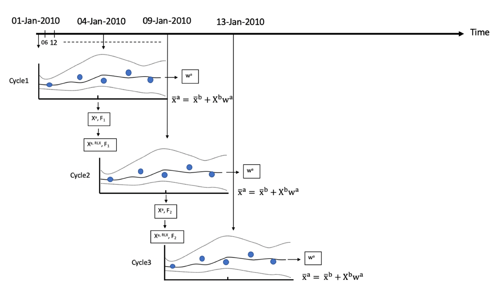
Figure 1 Schematic represents the temporal evolution of the LETKF cycle. In the first assimilation window (Cycle 1), the dotted lines show the ensemble forecast of CH₄ concentrations (with two ensemble members), the solid line shows the linear combination of the forecasts, and the filled circles show the observations of CH₄ concentration. The data assimilation finds the linear combination of the ensemble forecast by estimating the weight (w^a) that best fits the observations throughout the assimilation window. The analysis weight is applied to obtain optimal surface fluxes (F) and the concentration of CH₄ at the intermediate time of the data assimilation window. The updated analyzed concentration ensembles are used as initial conditions after relaxation (X^a, RLX) (Eq. 8) for the next ensemble forecast. The spread of the ensemble members represents the forecast error. The schematic is adapted from Kalnay and Yang (2010) and Miyazaki et al. (2011).

2.1 Covariance inflation

The LETKF data assimilation needs variance inflation to mitigate the underdispersed ensemble. We tested three methods: fixed multiplicative (FM), relaxation-to-prior spread (RTPS), and adaptive multiplicative covariance inflation.

The fixed multiplicative (FM) inflation method (Anderson and Anderson, 1999) inflates the prior ensemble by inflating the background error covariance matrix P^b defined in Eq. (2) as

$$\begin{array}{}\text{(6)}& {\mathbf{P}}_{\inf }^{\mathrm{b}}=\mathit{\gamma }{\mathbf{P}}_{\mathrm{tmp}}^{\mathrm{b}},\end{array}$$

where ${\mathbf{P}}_{\mathrm{tmp}}^{\mathrm{b}}$ represents the temporary background error covariance matrix, which is inflated by a factor γ.

The other inflation methods used to prevent the reduction of ensemble spread are relaxation-to-prior perturbation (RTPP) (Zhang et al., 2004) and relaxation-to-prior spread (RTPS) (Whitaker and Hamill, 2012). The RTPP method relaxes the reduction of the ensemble spread after updating the ensemble perturbations, which blends the background and analysis ensemble perturbations as

$$\begin{array}{}\text{(7)}& {\mathbf{X}}_{\inf }^{\mathrm{a}}={\mathit{\alpha }}_{\mathrm{RTPP}}{\mathbf{X}}^{\mathrm{b}}+(\mathrm{1}-{\mathit{\alpha }}_{\mathrm{RTPP}}){\mathbf{X}}_{\mathrm{tmp}}^{\mathrm{a}},\end{array}$$

where α_RTPP denotes the relaxation parameter of the RTPP.

The RTPS inflation method relaxes the reduction of the ensemble spread by relaxing the analysis spread to prior spread as

$$\begin{array}{}\text{(8)}& {\mathbf{X}}_{\mathrm{RLX}}^{\mathrm{a}}=\left({\displaystyle \frac{{\mathit{\alpha }}_{\mathrm{RTPS}}{\mathit{\sigma }}^{\mathrm{b}}+\left(\mathrm{1}-{\mathit{\alpha }}_{\mathrm{RTPS}}\right){\mathit{\sigma }}^{\mathrm{a}}}{{\mathit{\sigma }}^{\mathrm{a}}}}\right){\mathbf{X}}_{\mathrm{tmp}}^{\mathrm{a}},\end{array}$$

where σ and α_RTPS denote the ensemble spread and relaxation parameter of the RTPS, respectively. The range of the α_RTPS parameter is bounded by [0, 1]. This study focuses mainly on the FM and RTPS covariance inflation methods.

In addition, Miyoshi (2011) applied adaptive inflation by determining the multiplicative inflation factors at every grid point at every analysis step using the observation-space statistics derived by Daley (1992) and Desroziers et al. (2005).

$$\begin{array}{}\text{(9)}& <d{d}^{\mathrm{T}}>=H{\mathbf{P}}_{\inf }^{\mathrm{b}}{H}^{\mathrm{T}}+\mathbf{R},\end{array}$$

where the operator “<⋅>” denotes the statistical expectation and $d=y^{\mathrm{o}}-H{\stackrel{\mathrm{‾}}{x}}^{\mathrm{b}}$ (observation minus first guess), and R is the error observation covariance matrix.

The impact of using the adaptive multiplication inflation method is discussed in the GOSAT synthetic observation assimilation experiments in Sect. 4.2.

2.2 MIROC4-ACTM

Model for Interdisciplinary Research on Climate, version 4.0 (MIROC4)-based ACTM (hereafter referred to as MIROC4-ACTM) (Patra et al., 2018; Bisht et al., 2021) is used here for CH₄ concentration simulations. The model simulations have been performed at a horizontal grid resolution of approximately 2.8 × 2.8^∘ latitude–longitude (T42 spectral truncations) and at hybrid vertical coordinates of 67 levels (Earth's surface to 0.0128 hPa; Watanabe et al., 2008). Bisht et al. (2021) performed multi-tracer analysis and demonstrated the importance of very well resolved stratosphere in the MIROC4-ACTM that illustrates better extratropical stratospheric variabilities and simulated tropospheric dynamical fields. The meteorological fields in MIROC4-ACTM are nudged to the JMA reanalysis (JRA-55) data (Kobayashi et al., 2015).

3 Experimental setup

3.1 Construction of known surface emissions (truth)

Present OSSEs intend to develop basic tuning strategies before the actual data to be assimilated, which is useful to accelerate the operational use of real observations. The OSSE has been discussed here by exploiting the known “truth”. The synthetic observations to be assimilated in the OSSE are generated from nature runs which use bottom-up surface emission (true) data to simulate global 3-D CH₄ concentrations. The true surface CH₄ emissions are prepared on the monthly scale using anthropogenic and natural sectors, minus the surface sinks due to bacterial consumption in the soil (Chandra et al., 2021). The anthropogenic emissions were obtained from the Emission Database for Global Atmospheric Research, version 4.3.2 inventory (EDGARv4.3.2) (Janssens-Maenhout et al., 2019), which includes the emissions from the major sectors, such as fugitive sources, enteric fermentation and manure management, and solid waste and wastewater handling. The biomass burning emissions are taken from the Global Fire Database (GFEDv4s) (van der Werf et al., 2017) and Goddard Institute for Space Studies emissions (Fung et al., 1991). The wetland and rice emissions are taken from the process-based model of the terrestrial biogeochemical cycle, Vegetation Integrated Simulator of Trace gases (VISIT) (Ito, 2019), which is based on Cao et al. (1996). Other natural emissions, such as those from the ocean, termites, and mud volcanoes are taken from the TransCom-CH₄ inter-comparison experiment (Patra et al., 2011). The total emissions are taken as the truth for the OSSEs, and the concentration simulated by MIROC4-ACTM will be referred to as synthetic observations.

3.2 Prior flux preparation and LETKF setting

Based on our understanding of CH₄ inverse modeling, the uncertainty in regional flux estimation is found to be 30 % or lower (Chandra et al., 2021). Therefore, we attempted to reproduce the true flux by starting with a prior flux that is lower than the true flux by 30 % (prior flux has the same seasonal cycles as true flux). The MIROC4-ACTM is initialized with a spin-up of 3 years (2007–2009) with prior flux distribution. The initial CH₄ distribution on 1 January 2007 was taken from an earlier simulation of 27 years. An initial perturbation with standard deviation of approximately 6 %–8 % spread is applied to the a priori flux as the initial ensemble spread, whereas no ensemble perturbation was applied to the initial CH₄ concentration. The sensitivity of the initial ensemble spread to CH₄ flux estimation is discussed in Sect. 4.2. The uncertainty to perturb prior fluxes is generated based on random positive values with normal distribution. The monthly scale prior emission is linearly interpolated at 6-hourly intervals to be used in the MIROC4-ACTM simulation for data assimilation. This study performs two LETKF data assimilation experiments. In these experiments, we provided initial perturbation on a regional basis over land (53 different land regions; Chandra et al., 2021), and at every grid over ocean, no spatial error correlation between grid points is considered among ensemble members. However, in Sect. 4.2.5, we also discussed the sensitivity of CH₄ data assimilation by providing the initial ensemble spread at every grid by considering the horizontal spatial error correlation between grid points among ensemble members, with a global mean correlation of 20 %.

3.3 Experiment 1: synthetic dense observation formulation

The OSSE setting with very accurate and dense observation surface data is an attempt to demonstrate that the data assimilation system works reasonably in the estimation of the true surface flux. Errors in the estimated flux could arise due to the insufficient ensemble size and also the implemented inflation methods to overcome the undersampling, along with a simplified forecast process of the emissions. In real data assimilation, there are additional sources of potential errors, such as atmospheric transport and inappropriate prior or observation uncertainties. In our OSSEs, CH₄ fluxes as mentioned in Sect. 3.2 are used as “true” fluxes in generating synthetic observations (CH₄ concentrations). In Experiment 1, the simulated surface layer CH₄ concentrations at each grid for the entire globe were used as synthetic observations. We added a constant measurement uncertainty of 5 ppb, which is typically achieved by the present-day measurement systems (e.g., Lan et al., 2022).

In this study, the CH₄ observations are assimilated by applying the observation error covariance localization (Kotsuki et al., 2020) to reduce the spurious spatial correlation due to a smaller ensemble size than the degrees of freedom of the system ($\mathbf{R}\leftarrow \mathbf{R}\times \exp (-\frac{\mathrm{1}}{\mathrm{2}}\mathit{\{}{\left(d_{\mathrm{h}}/{\mathit{\sigma }}_{\mathrm{h}}\right)}^{\mathrm{2}}+{\left(d_{\mathrm{v}}/{\mathit{\sigma }}_{\mathrm{v}}\right)}^{\mathrm{2}}\mathit{\left\}}\right)$), where d_h and d_v denote the horizontal distance (km) and vertical difference (log[Pa]) between the analysis model grid point and observation location. The tunable parameters σ_h and σ_v are the horizontal localization scale (km) and vertical localization scale (log[Pa]), respectively. Using the spatial localization technique, we have estimated the CH₄ flux for each grid by choosing the CH₄ observations that influence the grid point using an optimal cutoff radius ($\simeq \mathrm{3.65}{\mathit{\sigma }}_{\mathrm{h},\mathrm{v}}$; Miyoshi et al., 2007) with a horizontal covariance localization (σ_h) of 2200 km and a vertical covariance localization (σ_v) of 0.3 in the natural logarithmic pressure (log[Pa]) coordinate. The localization is performed to improve the signal-to-noise ratio of ensemble-based covariance. Numerous sensitivity experiments have been performed by varying the horizontal and vertical localization length in order to obtain the optimized CH₄ flux that best compares with the truth. The LETKF assimilates the observations within the specified radius to solve the analysis state at each grid point independently (Liu et al., 2016; Kotsuki et al., 2020). The state vector of the analysis includes the atmospheric CH₄ concentration, which is the prognostic variable of forecast model, and the state vector is further augmented by the surface CH₄ flux, which is not a model prognostic variable. This augmentation enables the LETKF to directly estimate the parameter through the background error covariance with observed variables (Baek et al., 2006). The state vector augmentation is implemented similar to that used by Miyazaki et al. (2011). This approach analyzes CH₄ flux during the analysis step. The purpose of the simultaneous CH₄ emission and concentration optimization is to reduce the uncertainty of the initial CH₄ concentrations on the CH₄ evolution during the assimilation window and to maximize the observations potential (Tian et al., 2014).

The atmospheric CH₄ concentration is changed during both the analysis and forecast steps. A challenge of this scheme is that the analysis increment is added to the model state at each analysis step, without considering the global total CH₄ mass conservation in the model but consistent with the observed local CH₄ abundance.

In this case, the surface flux at every model grid point is analyzed with an 8 d assimilation window during the year 2010 with 100 ensemble members. The ensemble size and assimilation window are chosen based on the CH₄ flux estimation accuracy calculated by performing a sensitivity experiment for the ensemble size (60, 80, and 100) and assimilation window (3 and 8 d), respectively (not shown).

3.4 Experiment 2: synthetic satellite observation formulation

One way to address the real-world CH₄ flux estimation problem is to first make the OSSE dataset like real observations. In this OSSE, we have assimilated synthetic column-averaged CH₄ concentrations with a coverage mimicking GOSAT satellite observations. We prepared a model-simulated column-averaged CH₄ concentration (XCH₄) dataset that is spatiotemporally sampled with GOSAT observations as follows:

$$\begin{array}{}\text{(10)}& {\mathrm{XCH}}_{\mathrm{4}}={\mathrm{XCH}}_{\mathrm{4}\left(\text{a priori}\right)}+\sum _j{h}_j{a}_j({\mathrm{CH}}_{\mathrm{4}\left(\mathrm{ACTM}\right)}-{\mathrm{CH}}_{\mathrm{4}\left(\text{a priori}\right)}{)}_j,\end{array}$$

where XCH₄ is the column-averaged model-simulated CH₄ concentration. XCH_{4(a priori)} is a priori column-averaged concentration. CH_4(ACTM) and CH_{4(a priori)} are the CH₄ profile from ACTM and a priori, respectively. h_j is the pressure weighting function (j is the vertical layer index), and a_j represents the averaging kernel matrix for the column retrieval, which is the sensitivity of the retrieved total column at the various (“j”) atmospheric levels. In the next step, we added the same retrieval (XCH₄) error as GOSAT to the XCH₄ (ACTM-simulated) to make the OSSE more realistic and then attempt to estimate the true fluxes.

In this case, the CH₄ flux has been estimated for each grid by choosing the CH₄ observation with a cutoff radius ($\simeq \mathrm{3.65}{\mathit{\sigma }}_{\mathrm{h},\mathrm{v}}$), with a horizontal covariance localization (σ_h) of 5000 km and a vertical covariance localization (σ_v) of 0.35 in the natural logarithmic pressure (log[Pa]) coordinate. The optimal horizontal and vertical covariance localization values are chosen based on a trial-and-error method (those with the best fits to estimate the CH₄ flux when compared with truth). A long cutoff radius has been chosen due to sparse observational coverage of GOSAT. Covariance localization is necessary to remove long-range erroneous correlations and for mitigating sampling errors in the ensemble-based error covariance with a limited ensemble size (Miyoshi et al., 2007; Greybush et al., 2011; Kotsuki et al., 2020). The surface flux is analyzed at every model grid point with an 8 d assimilation window and 100 ensemble members; they are chosen based on the sensitivity experiments discussed in Sect. 4.2.

4 Results and discussion

4.1 Experiment with dense OSSEs

The time series of normalized root mean square error (RMSE; $\sqrt{{\sum }_{i=\mathrm{1}}^n(x_i^{\mathrm{a}}-x_i^{\mathrm{t}}{)}^{\mathrm{2}}/n}/{\stackrel{\mathrm{̃}}{x}}^{\mathrm{t}}$, where $x_i^{\mathrm{a}}$ and $x_i^{\mathrm{t}}$ are the analysis and true state at ith model grid point, n is the total number of grid points, and ${\stackrel{\mathrm{̃}}{x}}^{\mathrm{t}}$ represents the mean of true flux) in the analyses over the global landmass region is shown in Fig. 2. The normalized global RMSE is calculated using FM and RTPS inflation methods (Fig. 2) after assimilating synthetic observation at every grid (Sect. 3.4). Noteworthy is that the experiment with the FM inflation method shows 10 %–15 % larger error in estimating the atmospheric surface CH₄ flux compared to the RTPS inflation method. One of the reasons of the better RMSE using the RTPS inflation method is the higher number of degrees of freedom provided by relaxation (α_RTPS) in the ensemble spread (Eq. 8) that could nudge the ensemble of CH₄ concentrations towards observations. The initial flux analysis spread using RTPS and FM is shown in the Supplement (Fig. S1) and shows larger initial analysis flux spread over Brazil, tropical America, and Asia in RTPS inflation compared to the FM inflation method. We performed numerous sensitivity tests with the RTPS inflation method and found that uniform relaxation is not substantial for some of the regions. Figure 2 shows the RMSE for FM, fixed RTPS (α_RTPS=0.4; applied globally, the optimized value is obtained by manual fine-tuning), and conditional RTPS (α_RTPS=0.3–0.7 applied different α_RTPS values regionally by manual fine-tuning). In the case of conditional RTPS, the optimal values of α_RTPS, i.e., 0.6, 0.3, and 0.7 for the regions south of 20^∘ S, 20^∘ S–20^∘ N, and north of 20^∘ N, respectively, were obtained from data assimilation sensitivity calculations with varying α_RTPS values for the three regions separately to best match the true states. We find that the conditional RTPS method improves the accuracy by ∼ 5 % compared to fixed RTPS and 10 %–15 % compared to FM. In the following, we discuss the results obtained using the conditional RTPS and FM inflation methods.

We have also shown the RMSE (not normalized) of the surface flux in the Supplement (Fig. S2). The flux RMSE has been estimated globally for both the inflation methods and also for the region south of 20^∘ N (by considering only those land grids which fall in the region south of 20^∘ N; Fig. S2) for comparative purposes. It was noticed that (Fig. S2 in the Supplement), above north of 20^∘ N, the flux estimation error is higher, specifically during spring–summer when CH₄ emissions peak over most of the northern hemispheric regions (Fig. 3). The high uncertainty during spring–summer (Fig. S2) in the flux estimation over these regions could appear due to the attenuation of surface observations as a result of active vertical mixing. The RMSE during autumn (Fig. S2) is comparable in the case of the global region and the region south of 20^∘ N, which indicates that the RMSE is arising from southern hemispheric regions, likely over Brazil, as it peaks during autumn (Fig. 3).

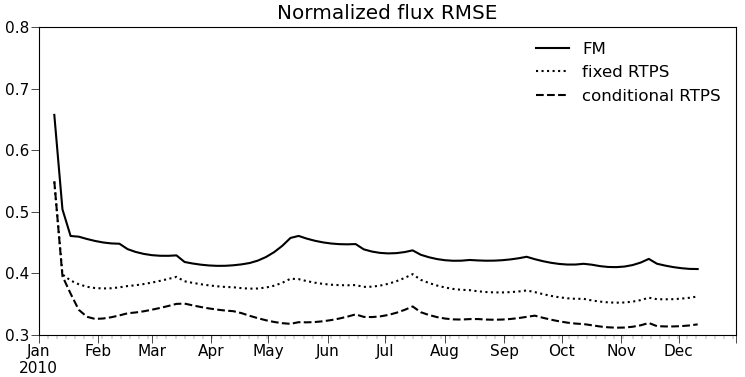
Figure 2 Time series of normalized RMSE of surface CH₄ flux analysis, for 1 year of data assimilation using FM, fixed RTPS, and conditional RTPS inflation methods over the global landmass region.

Figure 3 shows a regional total flux seasonal cycle comparison of the estimated fluxes for 15 terrestrial regions with the cycles of the prior and true fluxes. The estimated flux retrieved using RTPS inflation method over different regions agrees well with that of the true flux. We intend to show the capability of LETKF-estimated fluxes over these regions using surface observations to mimic the true fluxes in our understanding of the terrestrial biosphere CH₄ cycle. These results are consistent with Fig. 2, with an annual global normalized mean bias (${\sum }_{i=\mathrm{1}}^n(x_i^{\mathrm{a}}-x_i^{\mathrm{t}})/{\sum }_{i=\mathrm{1}}^n\left(x_i^{\mathrm{t}}\right)$) of −0.04. It can also be noticed from Fig. 3 that estimated fluxes converge to true fluxes over most of the regions after about 2–3 months.

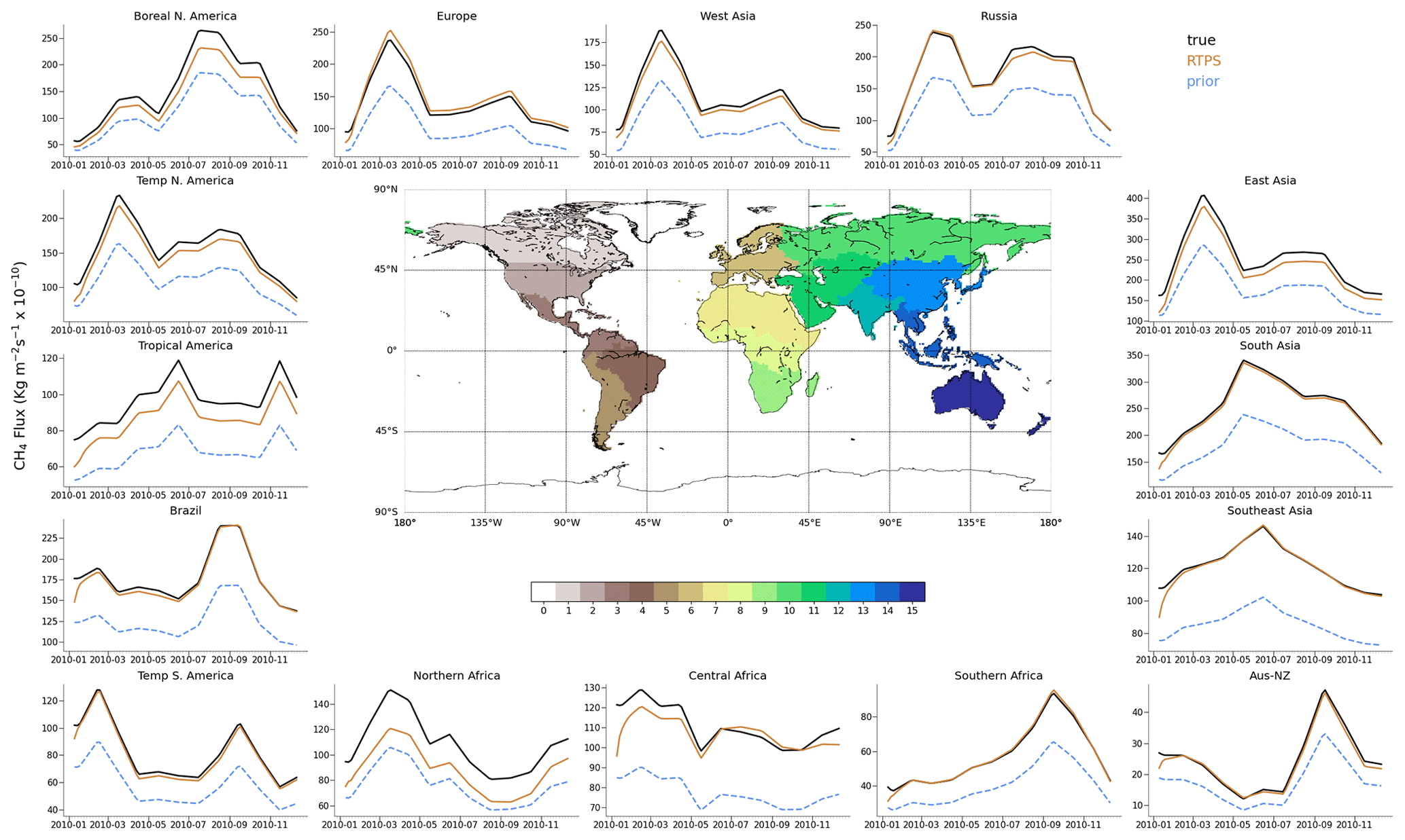
Figure 3 The 1-year CH₄ total flux seasonal cycles of the true flux (black), prior flux (blue), and flux estimated from the LETKF (orange) conditional RTPS inflation method in 15 regions after assimilating dense synthetic surface CH₄ observations.

To see the degree of similarity in the flux distribution between the estimated and true fluxes, we show monthly mean spatial flux distribution for June and November in Figs. 4 and 5, respectively, along with the bias in the prior and estimated flux. As shown in Figs. 4 and 5, the general spatial patterns of the true flux are estimated well. These results suggest that our LETKF system is capable of reproducing continental spatial flux patterns by using such idealized dense surface observational data. However, some clear differences in flux estimation could be noticed from the FM and RTPS inflation method (Figs. 4 and 5); e.g., over the Eurasian and American continent, analysis with RTPS shows clear improvement compared to the FM covariance inflation method. We calculated the global mean normalized bias with the RTPS and FM covariance inflation method, which is found to be −0.04 and −0.11, respectively, over land regions, and this showed that RTPS significantly improved the flux estimation compared to the FM covariance inflation method.

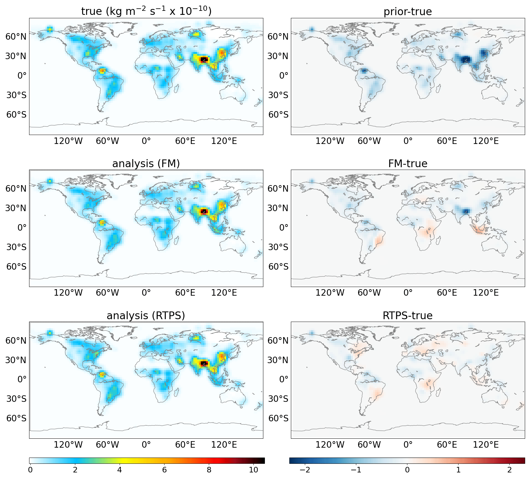
Figure 4 Spatial distribution of surface CH₄ fluxes (true; top left panel, FM analysis; middle left panel, RTPS analysis; bottom left panel) and the associated bias in prior (prior-true; top right panel) and estimated (FM-true; middle right panel, RTPS-true; bottom right panel) fluxes during June 2010.

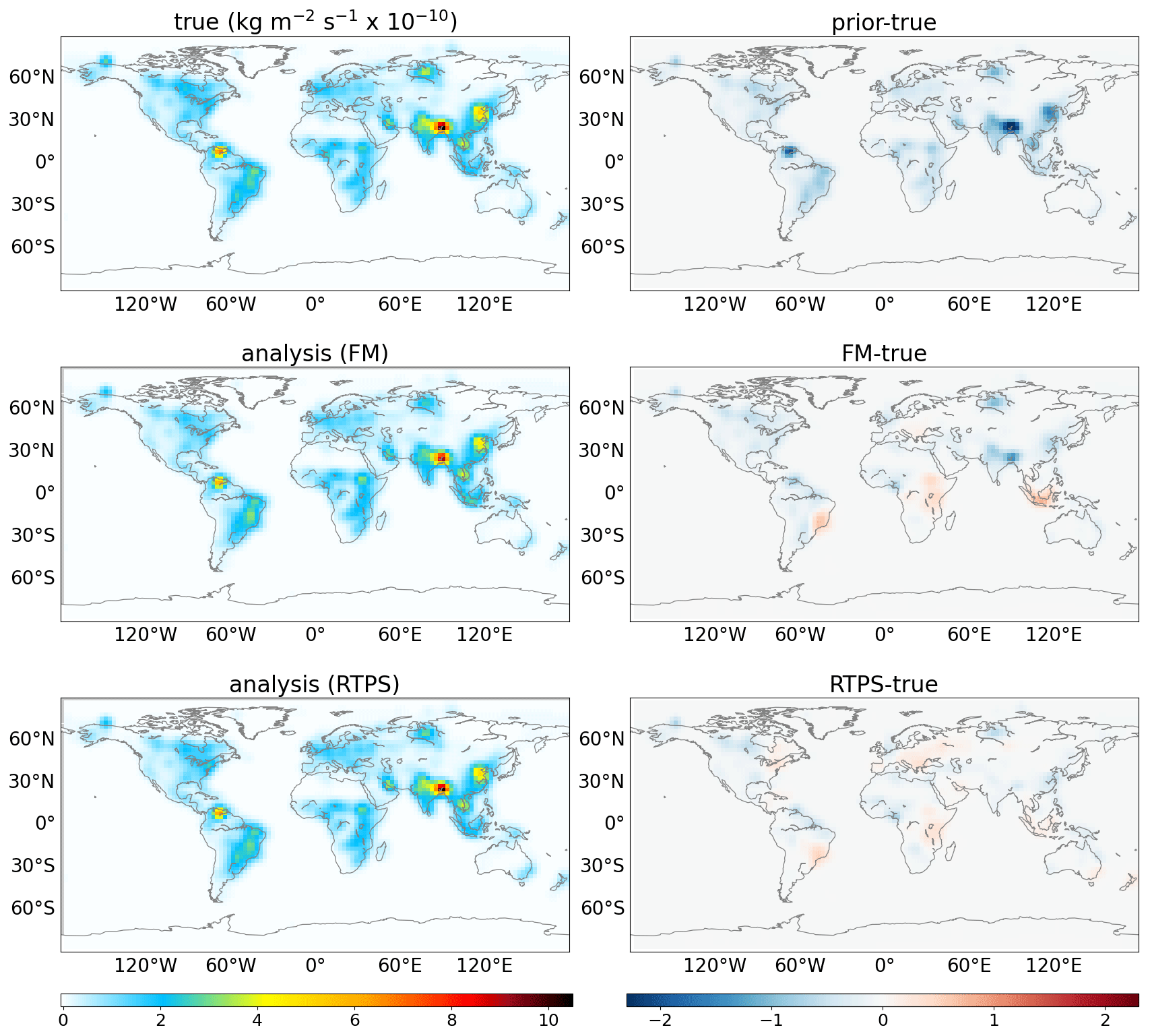
Figure 5 Same as Fig. 4 but for November 2010.

4.2 Experiment by mimicking the real satellite observational dataset

In this section we discuss the LETKF flux estimation by assimilation of GOSAT synthetic CH₄ concentration observations. Figure 6 shows the model-simulated mean XCH₄ concentration sampled spatiotemporally with GOSAT observations during January and July for the year 2010 (sampling method discussed in Sect. 3.4). In this case we have shown different LETKF sensitivity experiments, such as LETKF sensitivity to (1) FM, RTPS, and adaptive multiplicative inflation; (2) the assimilation window; (3) the ensemble size; (4) the χ² test; and (5) the prior ensemble spread. In the LETKF sensitivity experiments from 1–4, the initial ensemble spread employed a similar method to Experiment 1, and conditional RTPS inflation method is used. A conditional RTPS method is also used in Sect. 4.2.6 for CH₄ flux estimation.

4.2.1 LETKF sensitivity to FM, RTPS, and adaptive multiplicative inflation

This study mainly emphasizes FM and RTPS inflation methods used in CH₄ LETKF data assimilation. The annual average normalized RMSE (absolute bias) with RTPS and FM covariance inflation is found to be 0.59 (0.18) and 0.64 (0.22), respectively. The RTPS inflation method performs better than the FM inflation method overall. In addition to RTPS inflation, a sensitivity test is also performed using an adaptive multiplicative inflation method.

In the adaptive inflation, we need to provide an initial multiplicative inflation factor at the beginning of data assimilation cycle (Cycle 1 in Fig. 1). Following the method of Miyoshi (2011), the multiplication inflation factor information calculated in the previous cycle (i.e., Cycle 1 in Fig. 1) is used for the next data assimilation cycle at every grid point (Cycle 2 in Fig. 1). We perform two sensitivity experiments. In the first (second) case, we provided 50 % (40 %) initial inflation in the beginning of Cycle 1 (Fig. 1). The normalized RMSE in the both the adaptive inflation sensitivity experiments is comparable (0.65, Supplement Fig. S3a) till July, but from the beginning of August, the RMSE increases exponentially in the first experiment. However, in terms of the χ² distribution, CH₄ flux estimation with the first sensitivity adaptive multiplicative inflation experiment (50 % initial inflation case) is better than with the second sensitivity experiment (Supplement Fig. S3b; χ² test described in Sect. 4.2.4). To identify the regions of high estimated CH₄ flux error, we have shown the background error spread in CH₄ flux estimation over 15 regions (Supplement Fig. S3c) and found that the spread over west and southeast Asia rises exponentially post-July, which indicates the rise of estimated CH₄ flux error over these regions in the first sensitivity adaptive multiplicative inflation experiment. Our analysis suggests that CH₄ flux estimation depends on the initial inflation factor provided in the beginning of the data assimilation cycle (Cycle 1, Fig. 1) in the adaptive multiplication method. Also, we need to be very careful to monitor the background error spread evolution with time to estimate the CH₄ flux with adaptive inflation; the χ² distribution analysis is not sufficient.

In the case of RTPP inflation, we found the parameter α_RTPP is very difficult to fine-tune due to its very high sensitivity to estimating the CH₄ flux. We fail to obtain an optimized α_RTPP value to estimate the CH₄ flux. Whitaker and Hamill (2012) also demonstrated the better accuracy of the LETKF meteorological data assimilation with RTPS compared to the RTPP covariance inflation method. They found the RTPP method produces very large errors if the inflation parameter exceeds the optimal value.

4.2.2 Assimilation window

The LETKF data assimilation window length determines the time span of the observations assimilated in each assimilation cycle. We have shown the sensitivity of two assimilation window size configurations, 3 and 8 d, in the Supplement Fig. S4. Our sensitivity experiments with window size configurations show that the 8 d long assimilation window estimates the CH₄ flux with better accuracy (∼ 10 %) compared to the 3 d assimilation window because more observational information is incorporated into the system with the 8 d long assimilation window. This study uses an 8 d assimilation window for CH₄ LETKF data assimilation.

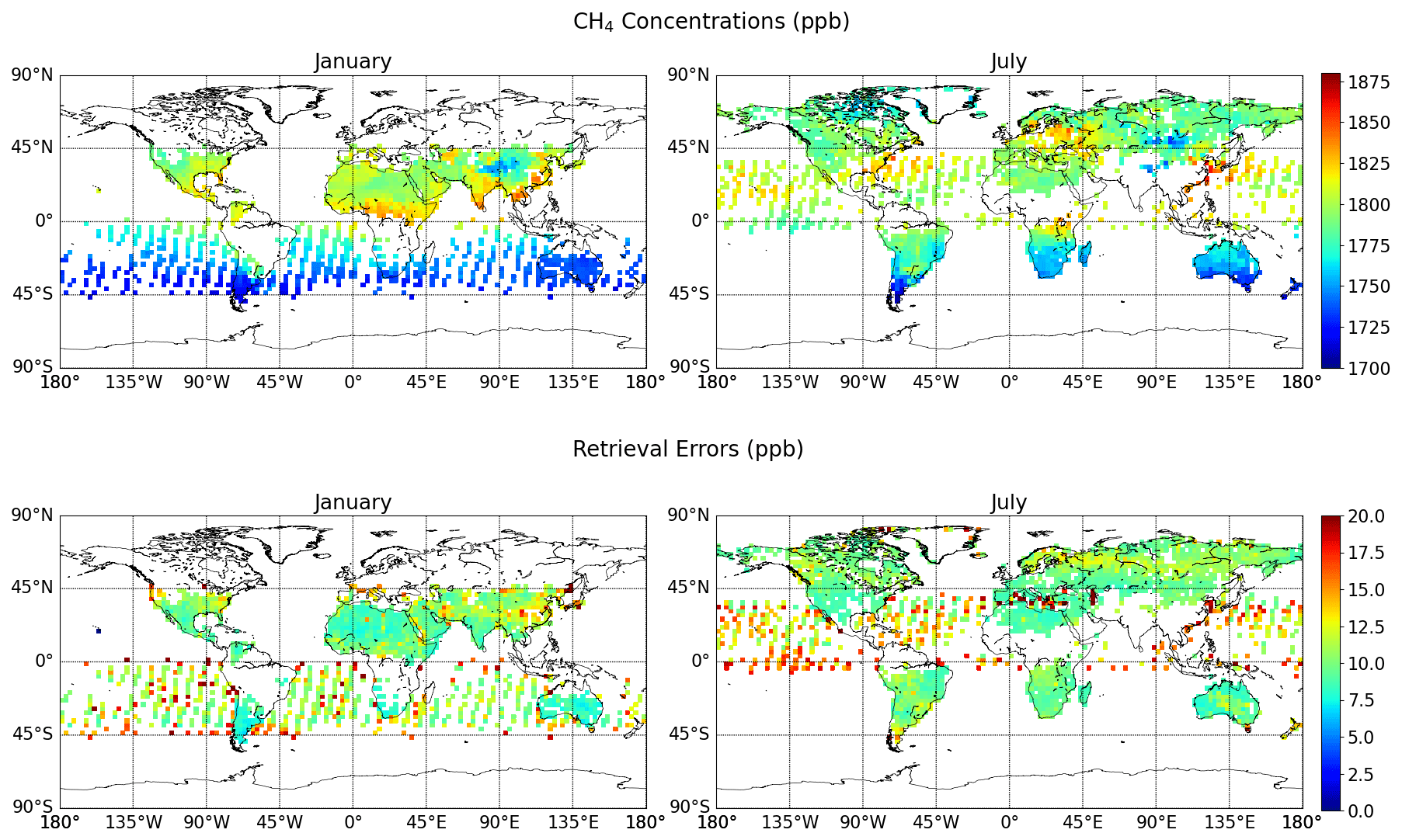
Figure 6 Monthly mean ACTM-simulated XCH₄ (ppb) sampled with GOSAT observations to be assimilated (valid during the year 2010). The actual retrieval errors are added in the synthetic GOSAT observations. Data are shown for 2 representative months, depicting the Southern and Northern Hemisphere differences in data coverage.

4.2.3 Ensemble size

Figure 7a shows the RMSE using different ensemble members. The RMSE stabilizes gradually as the ensemble size increases from 60 to 80 to 100 ensemble members. The ensemble size dependency of flux estimation suggests the further scope of the improvement in flux estimation by increasing the ensemble members. In this study we stick to 100 ensemble members due to high computational cost while solving large covariance matrices. The larger error in flux estimation in the case of column-averaged synthetic GOSAT CH₄ observations assimilation compared to dense observations (Fig. 2) is likely due to the weaker constraint on surface fluxes provided by satellite observations and sparse observations.

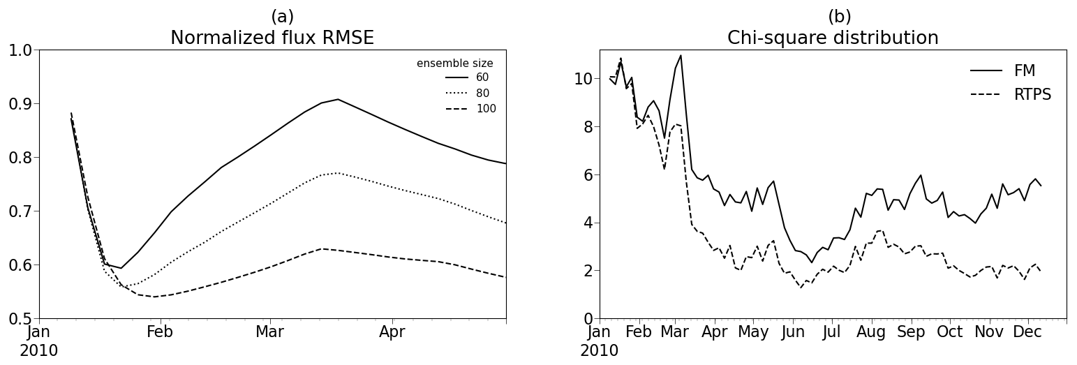
Figure 7 (a) Flux estimation RMSE using different ensemble sizes with RTPS covariance inflation. (b) χ² distribution using FM and RTPS covariance inflation methods, with an ensemble size of 100.

4.2.4 χ² test

We have carried out a χ² test for the evaluation of background error covariance matrix (Miyazaki et al., 2012). For the χ² test, the innovation statistics are diagnosed from the observation minus forecast (y^o−Hx^b), the estimated error covariance in the observation space (HP^bH^T+R), and the number of observations k as

$$\begin{array}{}\text{(11)}& Y={\displaystyle \frac{\mathrm{1}}{\sqrt{k}}}{\left(H{\mathbf{P}}^{\mathrm{b}}{H}^{\mathrm{T}}+\mathbf{R}\right)}^{-\mathrm{1}/\mathrm{2}}\left(y^{\mathrm{o}}-H{\mathbf{x}}^{\mathrm{b}}\right).\end{array}$$

Using this statistic, the χ² is defined as follows:

$$\begin{array}{}\text{(12)}& {\mathit{\chi }}^{\mathrm{2}}={\mathrm{traceYY}}^{\mathrm{T}}.\end{array}$$

The performance of the background error covariance matrix is determined based on the high and lower value of χ². The χ² value should converge to 1; a value higher (lower) than 1 indicates underestimation (overestimation) of the background error covariance matrices. Our results suggest that the background error covariance matrix is highly underestimated in both RTPS and FM covariance inflation methods (Fig. 7b). However, the χ² values' convergence towards 1 is better in the case of RTPS compared to the FM covariance inflation method, which indicates the improved representation of background errors and then more appropriate data assimilation corrections in the case of the RTPS inflation method. The χ² distribution starts saturating after the month of March. Post-March analysis shows the background error covariance matrix underestimation is much higher (>100 %) in the case of FM compared to the RTPS covariance inflation method.

4.2.5 CH₄ LETKF sensitivity to the initial ensemble spread

A test case for CH₄ LETKF data assimilation has been performed, where the initial spread is provided by considering the initial perturbation on each model grid with spatial error correlation between grid points among ensemble members, with a global mean correlation of 20 %. In this case, we found that the analysis fluxes are extremely sensitive to the initial ensemble spread if prior fluxes are perturbed with more than 5 % prior uncertainty. Therefore, we used initial ensemble perturbation with only 2 % prior uncertainty. Reducing the initial ensemble spread reduces the CH₄ flux estimation sensitivity (>60 %). However, it also poses a challenge to mitigate the underdispersed background error covariance matrix. We performed LETKF data assimilations in this case with the RTPS covariance inflation method (α_RTPS=0.9 optimized value is used here uniformly) with an 8 d long assimilation window and 100 ensemble members and calculated the normalized RMSE between the analysis and true fluxes (Supplement Fig. S5). It is noteworthy that the estimated error between the analysis and true fluxes (Fig. S5) with this setting (grid-wise initial ensemble spread) is still larger (25 %) than the case when the region-wise initial ensemble spread is used (Fig. 7a; 100 ensemble size). It suggests that initial ensemble spreads among ensemble members need to be meticulously chosen so that they best represent CH₄ variability among ensembles to estimate the CH₄ flux.

Note that the OSSEs used in this study did not consider the effects of model errors other than CH₄ fluxes, such as model transport errors. In real situations, model errors can have a substantial impact on flux estimates (Locatelli et al., 2013), which needs to be taken into account in background covariances. Therefore, the optimal data assimilation setting can differ between the OSSEs presented in this study and real observation cases. Further efforts, e.g., by conducting a more comprehensive OSSE that accounts for various model errors and by performing various sensitivity calculations in real cases, would provide an improved understanding of the optimal inflation settings to improve CH₄ flux estimates in following study.

4.2.6 Estimated CH₄ flux analysis

Figure 8 shows the regional flux seasonal cycle comparison for the estimated fluxes over 15 terrestrial regions with the cycles of the prior and true fluxes. We have also shown assimilation results in the case of the FM inflation method in the Supplement (Fig. S6), which shows the flux estimation disagreement over more regions compared to the RTPS inflation method, e.g., for tropical and North America, the whole African continent, and Australia–New Zealand.

Figure 8 Same as Fig. 3 but after assimilating synthetic GOSAT observations.

We have shown the GOSAT observations in Figs. 6 and S7. We found very marginal flux estimation improvement over Central Africa after May (Fig. 8), which could be associated with the lower GOSAT coverage over this region (Fig. 6). On the other hand, over northern Africa, no improvement in flux estimation is found. In the case of dense OSSEs too (Fig. 3), we did not find satisfactory flux estimation over northern Africa, which is most probably related to the insufficient initial spread among ensemble members over this region (we used the same initial ensemble spread in both OSSE cases). Over Europe, GOSAT observations are remarkably fewer, specifically for the first few months (January–April; Supplement Fig. S7). Therefore, the flux update over Europe would be influenced by the observations from neighboring regions falling under the chosen cutoff radius that are mainly in northern Africa, where the flux estimation itself not satisfactory. It could also be noticed that the retrieval error added in this OSSE case is high over Europe (September–October; Supplement Fig. S7) and its adjacent sea (Mediterranean Sea; June–August), which could also affect the surface CH₄ flux estimation.

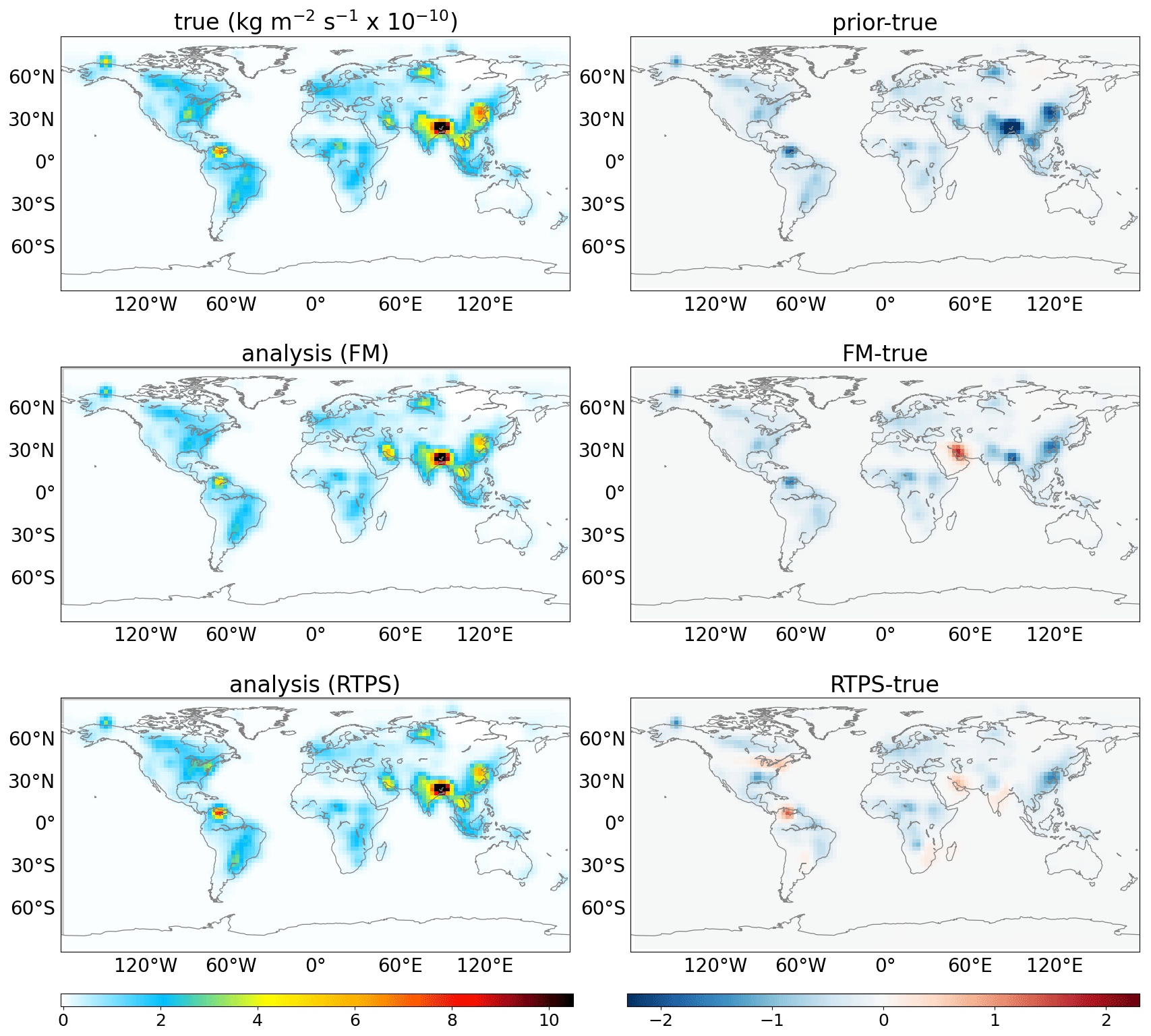
Figure 9 Monthly mean true (true; top left panel) and estimated (FM analysis; middle left panel, RTPS analysis; bottom left panel) CH₄ flux after assimilating column-averaged synthetic CH₄ concentrations (Fig. 6) during June using FM and RTPS inflation methods. The associated bias with prior and estimated fluxes is also shown (prior-true; top right panel; FM-true; middle right panel, RTPS-true; bottom right panel).

Figure 10 Same as Fig. 9 but for November.

Figures 9 and 10 show spatial patterns of the true and estimated fluxes by assimilating the column-averaged CH₄ concentrations during June and November (Fig. 6). It may be noticed that the RTPS covariance inflation method is more able to estimate the true flux pattern compared to the FM covariance inflation method. The spatial pattern shown using the RTPS inflation method emphasizes the positive and negative bias in the estimated flux (Figs. 9 and 10) but generally agrees with the flux seasonal cycle plots shown in Fig. 8.

Our LETKF CH₄ data assimilation experiment by assimilating GOSAT synthetic observation with the implementation of the advanced RTPS covariance inflation method better estimates the time-evolving surface CH₄ fluxes compared to the FM covariance inflation method. The difficulty to estimate the surface CH₄ flux over a few regions may be overcome by applying additional methodologies, such as the assimilation of surface observations simultaneously and the use of information about the CH₄ flux climatology. A correction factor derived based on empirical formulation that could use CH₄ flux climatology information is needed to apply to maintain the CH₄ mass conservation. This could be implemented by checking the simulated CH₄ burden gain between years in comparison with the observed CH₄ growth rates.

5 Summary

In this study, we have introduced a 4D-LETKF data assimilation system that utilizes MIROC4-ACTM as a forward model for CH₄ flux estimation. This study has extensively tested both FM and RTPS inflation methods for the LETKF CH₄ flux estimation. We have conducted two experiments to demonstrate the ability of LETKF system to estimate the CH₄ surface flux globally. In Experiment 1, we have assimilated the synthetic dense surface CH₄ observations, while in Experiment 2, synthetic GOSAT CH₄ observations are assimilated. Based on the results of the sensitivity tests using FM and RTPS inflation methods in Experiment 1, we have found that RTPS inflation produces significantly less normalized RMSE (10 %–15 %) compared to the FM inflation method. In Experiment 2, we discussed LETKF parameters, such as different inflation techniques, ensemble size, assimilation window, initial ensemble spread sensitivity, and χ² test. The ensemble size (this study uses maximum 100 ensemble members) sensitivity test suggests that more ensemble members could help to accurately represent the covariance matrix with a higher number of degrees of freedom. The assimilation window sensitivity test shows that an 8 d assimilation window reduces the normalized flux RMSE by about 10 % compared to a 3 d assimilation window in the case of GOSAT synthetic observations assimilation.

Our approach of assimilation with RTPS inflation could provide a higher number of degrees of freedom to fit the ensemble of CH₄ concentrations to the observed ones, resulting in the improved analyzed fluxes. The RTPS inflation method is capable of obtaining reasonable flux estimates with a normalized annual mean bias of 0.04 and 0.61 in the case of dense surface synthetic observations and GOSAT synthetic observations, respectively. We demonstrated in our sensitivity OSSE with synthetic GOSAT observations that, over American and African continents and also over Australia–New Zealand, the LETKF data assimilation with the FM inflation method does not show much improvement in the true flux estimation, but the RTPS inflation method reasonably estimates the true flux over most of these regions. One of the reasons for better flux estimates with the RTPS inflation method is the drastic prevention of analysis spread. In the CH₄ LETKF flux estimation, the surface CH₄ flux is not a prognostic state vector in the ACTM, which results in the continuous decay of spread in analysis steps. The RTPS inflation method could mitigate such an underdispersed spread problem. This study finds that spatially homogeneous relaxation is not sufficient. It needs to be fine-tuned and applied conditionally.

The sensitivity of LETKF CH₄ flux estimation to the initial ensemble spread needs to be carefully dealt with when applied to real data assimilation system. A future OSSE with an additive covariance inflation technique could be interesting while applied with the RTPS inflation method for CH₄ LETKF data assimilation since in additive covariance inflation, initial estimated flux error cannot propagate. The state vector augmentation technique used here updates the flux after each data assimilation cycle, but it does not conserve the total atmospheric CH₄ amount, which is one of the limitations of this work. A correction factor needs to be implemented to conserve the total atmospheric CH₄ amount after completion of a few data assimilation cycles. We have not accounted for the transport error due to meteorological fields in this work (Patra et al., 2011); in the case of real observation data assimilation, a week-long window may introduce transport errors in CH₄ analysis because of the nonlinear growth of ensemble perturbations.