the Creative Commons Attribution 4.0 License.
the Creative Commons Attribution 4.0 License.
 | 29 Mar 2023
A method for generating a quasi-linear convective system suitable for observing system simulation experiments
Jeremy A. Gibbs
Louis J. Wicker
To understand the impact of different assimilated observations on convection-allowing model forecast skill, a diverse range of observing system simulation experiment (OSSE) case studies are required (different storm modes and environments). Many previous convection-allowing OSSEs predicted the evolution of an isolated supercell generated via a warm air perturbation in a horizontally homogenous environment. This study introduces a new methodology in which a quasi-linear convective system is generated in a highly sheared and modestly unstable environment. Wind, temperature, and moisture perturbations superimposed on a horizontally homogeneous environment simulate a cold front that initiates an organized storm system that spawns multiple mesovortices. Mature boundary layer turbulence is also superimposed onto the initial environment to account for typical convective-scale uncertainties.
Creating an initial forecast ensemble remains a challenge for convection-allowing OSSEs because mesoscale uncertainties are difficult to quantify and represent. The generation of the forecast ensemble is described in detail. The forecast ensemble is initialized by 24 h full-physics simulations (e.g., radiative forcing, surface friction, and microphysics). The simulations assume different surface conditions to alter surface moisture and heat fluxes and modify the effects of friction. The subsequent forecast ensemble contains robust non-Gaussian errors that persist until corrected by the data assimilation system. This purposely degraded initial forecast ensemble provides an opportunity to assess whether assimilated environmental observations can improve, e.g., the wind profile. An example OSSE suggests that a combination of radar and conventional (surface and soundings) observations are required to produce a skilled quasi-linear convective system forecast, which is consistent with real-world case studies. The OSSE framework introduced in this study will be used to understand the impact of assimilated environmental observations on forecast skill.
- Article
(12909 KB) - Full-text XML
- BibTeX
- EndNote


Forecasts of convection can provide important guidance to forecasters ahead of an impending severe weather event; however, forecast skill is often limited because the predicted storms are sensitive to modest initial condition errors. To mitigate these errors, a combination of in situ (surface stations and radiosondes) and remotely sensed observations (e.g., radar reflectivity and satellite radiances) are blended with a prior estimate using data assimilation (Kalnay, 2002). Although skilled convection-allowing model (CAM) forecasts can be generated after assimilating commonly available observations (e.g., Johnson et al., 2013; Sobash et al., 2016; Skinner et al., 2018; Snook et al., 2019; Flora et al., 2019), much of the atmosphere at the meso- and convective scales remains unobserved. Most model state variables are also, at best, indirectly observed and thus a challenge to update during data assimilation. These limitations introduce uncertainties into the posterior estimate of the environment and degrade the forecast skill. To address these concerns, data assimilation experiments can be used to determine future observational networks that, when assimilated, positively impact CAM forecast skill.
Rather than prematurely deploying observing systems to conduct real-world experiments, which are costly and time-consuming, many studies rely on observation system simulation experiments (OSSEs) to determine the impact of assimilating new observation types (e.g., Snyder and Zhang, 2003; Xue et al., 2006; Jung et al., 2008; Yussouf and Stensrud, 2010; Potvin and Wicker, 2012; Sobash and Stensrud, 2013; Cintineo et al., 2016). These experiments assimilate simulated observations that are extracted from a nature run – a well-tuned simulation that is designed to resemble a real-world weather phenomenon (e.g., an isolated supercell, quasi-linear convective system or QLCS). OSSEs provide an elegant strategy to test the effectiveness of different observation types, deployment strategies, and sampling intervals because the simulated observations are easily reconfigured. OSSEs can also improve the assimilation system independently of the errors in the model physics (e.g., Zeng et al., 2021). To understand the impact of different observing network configurations, the data assimilation initialized forecasts are verified against the nature run. Despite the potential power of this framework, designing these experiments is nontrivial because both the nature run and model prior state must reflect complex atmospheric phenomena and uncertainties that are observed in the environment.
It is imperative to run forecast and data assimilation experiments for a diverse range of storm cases to ensure that OSSE results are robust. Despite many different observed storm modes (e.g., Gallus et al., 2008), most convective-focused OSSEs simulate the evolution of a supercell thunderstorm (e.g., Snyder and Zhang, 2003; Zhang et al., 2004; Dowell et al., 2004; Xue et al., 2006; Caya et al., 2005; Gao and Stensrud, 2014; Kerr et al., 2015; Zhao et al., 2021). This is done, in part, because supercell thunderstorms produce a disproportionately large number of severe weather and tornado reports (e.g., Kain et al., 2008) and thus serve as a logical first choice. These cases are also easier to create because a realistic storm can be generated by inserting a warm bubble into an unstable, highly sheared, and horizontally homogeneous environment.
Only a few OSSEs simulate the evolution of non-supercellular convection, such as disorganized convection (Potvin et al., 2013) or a line of storms that grows in scale (Sobash and Stensrud, 2013). To our knowledge, no idealized OSSE (i.e., experiments initialized from a sounding and a supplied mesoscale background) has simulated the evolution of a convective line initiated via a frontal boundary. QLCSs that initiate via frontal forcing in highly sheared but marginally unstable environments often cause severe weather in the southeastern United States during the cool season (Guyer and Dean, 2010; Sherburn and Parker, 2014; Sherburn et al., 2016). Creating OSSEs that simulate other convective initiation mechanisms (e.g., cold front and dry line boundary) and environments (e.g., high shear and low instability) will help us to better understand how assimilated observations impact the environment and the subsequent evolution of convection.
Convective-scale OSSEs and real-world case studies often use an ensemble Kalman filter (EnKF; Evensen, 1994, 2003) to create the forecast initial conditions (e.g., Snyder and Zhang, 2003; Dowell et al., 2004; Snook et al., 2011; Romine et al., 2013; Wheatley et al., 2015; Jones et al., 2016; Johnson and Wang, 2017). This strategy is preferred for CAM forecast experiments because the data assimilation system can update unobserved model state variables using flow-dependent error covariances derived from the forecast ensemble. The EnKF can also assimilate remotely sensed observations (e.g., radar reflectivity) and use cross-covariances to update environmental and in-storm fields (e.g., Snyder and Zhang, 2003). Experiments must craft a forecast ensemble that is representative of the event uncertainty to maximize the data assimilation system performance. This is challenging when the initial state is generated from a single or composite sounding. Therefore, a variety of strategies has been used to create the initial forecast ensemble. For example, random perturbations are commonly used to add variability to the initial environment. The perturbations are inserted into the environment as grid point noise (e.g., Snyder and Zhang, 2003; Tong and Xue, 2005; Dawson et al., 2012) or smooth, spatially correlated structures (e.g., Caya et al., 2005; Dowell and Wicker, 2009; Jung et al., 2012). The perturbation amplitude is calibrated to represent sources of uncertainty, including environmental variability (e.g., Dawson et al., 2012) and model error (e.g., Cintineo and Stensrud, 2013). While these perturbations are calibrated to account for sources of ensemble uncertainty, they remain an ad hoc technique used to introduce uncertainty into the forecast. The evolution of the ensemble spread is sensitive to many user-defined parameters, including perturbation length scale, amplitude, and location (e.g., Snyder and Zhang, 2003; Dowell et al., 2004; Caya et al., 2005).
Despite being commonly used, random initial condition perturbations are not necessarily representative of the forecast errors observed in real-world case studies. Many studies assume that the perturbations are unbiased and have little impact on the mean ensemble environment. This contradicts many previous CAM studies that note that model errors bias the forecast environment (e.g., Snook and Xue, 2008; Coniglio et al., 2013; Romine et al., 2013; Cohen et al., 2015). Since the ensemble mean environment closely matches the observed truth, OSSEs are unable to determine what impact assimilated environmental observations (e.g., surface stations and aircraft soundings) could have on the storm forecasts. To confront this challenge, some studies strategically bias the forecast initial environment (e.g., Stratman et al., 2018) or purposely fail to initiate convection (e.g., Kerr et al., 2015) to ensure a greater disparity between the nature run simulation and forecasts. Although these studies better represent forecast biases observed in real-world case studies, there remain few options to introduce appropriate forecast biases in an OSSE.
A diverse set of OSSE cases that challenge the effectiveness of our data assimilation systems is required to holistically understand the impact that observing systems can have on CAM forecasts. The goal of this study is to provide a novel OSSE framework to understand how assimilated observations impact the forecast performance. This study provides instructions to create an OSSE for a QLCS that initiates along a frontal boundary in a high-shear, low-instability environment. Techniques to create the initial ensemble of simulations, which rely on uncertainties introduced by model physics, are also introduced. These techniques lead to a purposely degraded initial ensemble that contains robust non-Gaussian errors, such that the profiles from the nature run are often out of the ensemble spread. This ensemble of simulations allows for an evaluation of the data assimilation system described herein. The steps taken to create the nature run and forecast ensemble are listed in Sects. 2 and 3. Sections 4 and 5 describe the data assimilation procedure and forecast verification metrics. An example OSSE is described in Sect. 6, and Sect. 7 discusses the use of this OSSE framework for future studies.
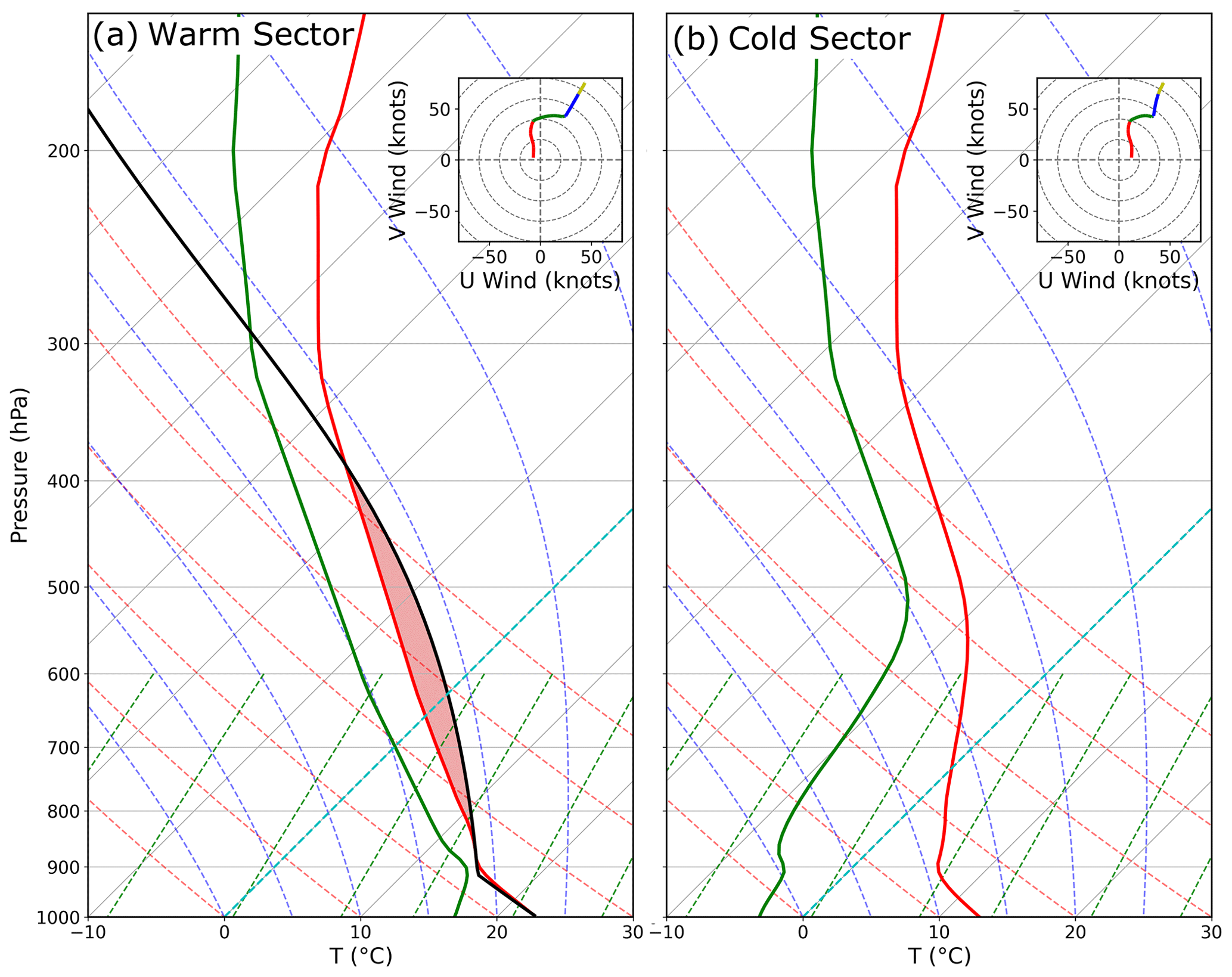
Figure 1(a) The initial sounding for the nature run simulation. Vertical red lines and green lines correspond with T and Td. The vertical black line marks the temperature of an air parcel launched from the surface. The hodograph, which is plotted in the upper-right corner, is color coded by height above ground level (a.g.l.), and 0–1 km is red, 1–3 km is green, 3–5 km is blue, and 5–10 km is yellow. Both soundings also initialize the (a) warm sector and (b) cold sector simulations that create the forecast ensemble.
The following steps are taken to create the nature run simulation for this case:
-
Step 1. Initialize the environment using a high-shear, low-CAPE (convective available potential energy) composite sounding (Fig. 1a) and insert a frontal boundary on the western edge of the domain.
-
Step 2. Conduct a separate initial turbulence simulation to generate realistic perturbation fields of temperature, wind, and moisture.
-
Step 3. Superimpose the resultant turbulence fields on the initial conditions created in step 1 to generate the final environment used to start the nature run simulation.
The remainder of this section explains, in depth, the procedure used to generate the nature run simulation.
2.1 Initial environment
The nature run is initialized with a horizontally homogeneous environment using a high-shear, low-CAPE composite sounding. The initial sounding (Fig. 1a), introduced by Sherburn and Parker (2019), is modified in the lower troposphere to support the development of robust boundary layer turbulence. High-shear, low-CAPE environments, which support approximately half of the significant (EF2+) tornadoes in the contiguous United States (Schneider et al., 2006), are the primary target of the Verification of the Origins of Rotation in Tornadoes Experiment Southeast (VORTEX-SE) field experiments. OSSEs initialized with this environment should help determine which observing systems benefit the forecast skill the most and how to appropriately deploy them (e.g., spatial and temporal density).

Figure 2Nature run initial conditions at the lowest model level for (a) T, (b) Td, and (c) u wind. The plotted subdomain is centered on the initial frontal boundary.
A cold front provides the mechanical forcing required to initiate sustained convection for this case. Potential temperature (θ), dew point temperature (Td), and u wind perturbations of −10 K, −20 K, and 10 m s−1, respectively, are inserted along the western domain edge to create the frontal boundary. Perturbation magnitude fp(x) decreases with distance from the western and bottom domain boundaries, following a cosine function:
where
and x, y, and z are the distance of a grid point from the western, southern, and bottom boundaries, respectively. The assumed frontal width is 100 km, and the height is 6 km. These equations generate a north–south front that, left undisturbed, will cause storms to initiate at the same time for an east–west location. Waves are added to the frontal boundary in the north–south direction to vary the convective initiation timing and location via the following:
where λ is the wavelength (100 km), ϕ is the phase shift (0), and δ is the wave amplitude (10 km). The subtle frontal waves (Fig. 2) simulate the natural variability observed in the frontal location.
2.2 Boundary layer turbulence
Boundary layer turbulence plays an important role in the evolution of convection. Storm interactions with turbulent eddies can modify the mesocyclone circulation in addition to the storm intensity and location (e.g., Nowotarski et al., 2015; Markowski, 2020; Labriola and Wicker, 2022). Turbulent eddies transport near-surface air further aloft and impact boundary layer temperature, wind, and moisture profiles. The turbulence also facilitates the downward transport of high-momentum air aloft and is consequently necessary to properly simulate the effects of surface friction on thunderstorm evolution (Markowski, 2016). To enhance the realism of the experiment, the nature run simulation for this case is initialized with fully mature boundary layer turbulence, using a technique introduced by Markowski (2020) and subsequently improved upon by Labriola and Wicker (2022).
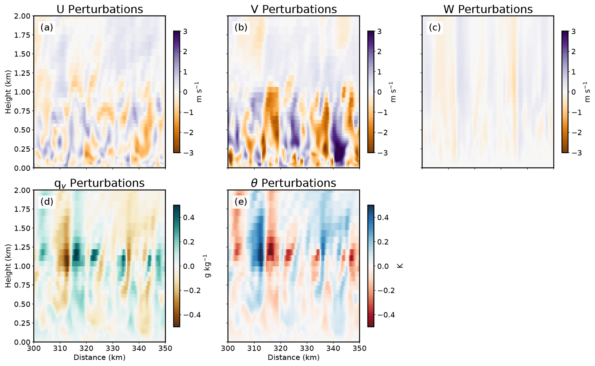
Figure 3Vertical cross sections of boundary layer turbulent perturbations that are inserted into the nature run simulation. Plotted fields include the (a) u, (b) v, and (c) w components of wind, (d) qv, and (e) θ.
A turbulence simulation is first conducted to create a realization of the boundary layer turbulence. The turbulence simulation is initialized with the nature run initial sounding (Fig. 1a), and then small-scale, pseudo-random θ perturbations (±0.25 K) are superimposed on the initial environment to initiate turbulence. The settings and grid configuration used for the turbulence simulation are nearly identical to those used for the nature run (see Sect. 2.3), with a few notable exceptions. The lateral boundary conditions are made periodic so that turbulent eddies persist across domain boundaries. The turbulence simulation assumes no radiative forcing, no surface friction, and applies Coriolis acceleration to the perturbation wind field. These settings are necessary to form robust turbulent motions (Fig. 3) without spawning spurious convection or substantially modifying the initial environment (see Labriola and Wicker, 2022, for more details). As the turbulence simulation is integrated 12 h forward in time, the random perturbations evolve to form a turbulent boundary layer (Fig. 3). At the conclusion of the turbulence simulation, the perturbation, u, v, w, θ, and water vapor mixing ratio (qv) fields (i.e., the difference between a model state variable and the horizontal planar mean) are superimposed on the initial conditions used for the nature run. These perturbations do not statistically impact the nature run's mean initial environment because they average to 0 across the domain.
2.3 Prediction model settings
The nature run simulation for this case is created using the Cloud Model 1 (CM1; Bryan and Fritsch, 2002; Bryan and Rotunno, 2009) release 20.1. The simulation is run between 00:00–08:00 UTC on 1 January 2021 on a domain centered over Jackson, Mississippi (32.30∘ N, −90.18∘ W). This time and location correspond with previous cold-season tornadic events that occurred in the southeastern United States (Sherburn and Parker, 2014). The numerical mesh is 1200×600 computational points in the x and y directions, respectively, with a uniform horizontal grid spacing of 500 m. This grid spacing, which is too coarse to fully resolve large turbulent eddies (Bryan et al., 2003), was selected as a balance between the computational feasibility and physical realism of the boundary layer turbulence. Lateral boundary conditions are open in the x direction, to preserve the east–west temperature gradient, and periodic in the y direction. No Coriolis acceleration is assumed due to the complex nature of the atmospheric flow associated with the frontal boundary.
The 120-level vertical grid is stretched from 10 m at the lowest model level to 250 m at heights between 9.875–15 km (i.e., the model top). The simulation is run with a semi-slip bottom boundary condition and uses the Jiménez et al. (2012) surface layer scheme to calculate surface fluxes and surface stress. The upper boundary condition is free slip, and Rayleigh damping is applied with a coefficient of 0.003 s−1, starting at 12 km above ground level (a.g.l.).
Model physics options for this case were selected to ensure that the simulation accurately portrays the evolution of a storm system. Precipitation processes are parameterized using the double-moment Morrison microphysical parameterization (Morrison et al., 2005, 2009). The microphysical parameterization predicts the evolution of a single rimed ice species similar to hail (e.g., dense and faster fall speeds), which produces realistic squall line simulations (Bryan and Morrison, 2012). No separate cloud parameterization is used. The NASA Goddard radiative scheme simulates the effects of longwave and shortwave radiative forcing during the simulation period. Subgrid-scale (SGS) turbulence is parameterized using the Deardorff (1980) three-dimensional turbulence kinetic energy scheme.
2.4 Simulation results
The nature run setup produces a QLCS that persists for several hours before exiting the experiment domain (Fig. 4). Although the cold-air perturbation alone can initiate robust convection (e.g., Sherburn and Parker, 2019; Labriola and Wicker, 2022), the positive u wind perturbation along the western domain boundary is necessary to sustain convection. The post-frontal winds advect cold air eastward with time (Fig. 4a, c, e) and maintain strong temperature and moisture gradients along the boundary. The wind perturbation also enhances convergence, which initiates and sustains the robust storm system.
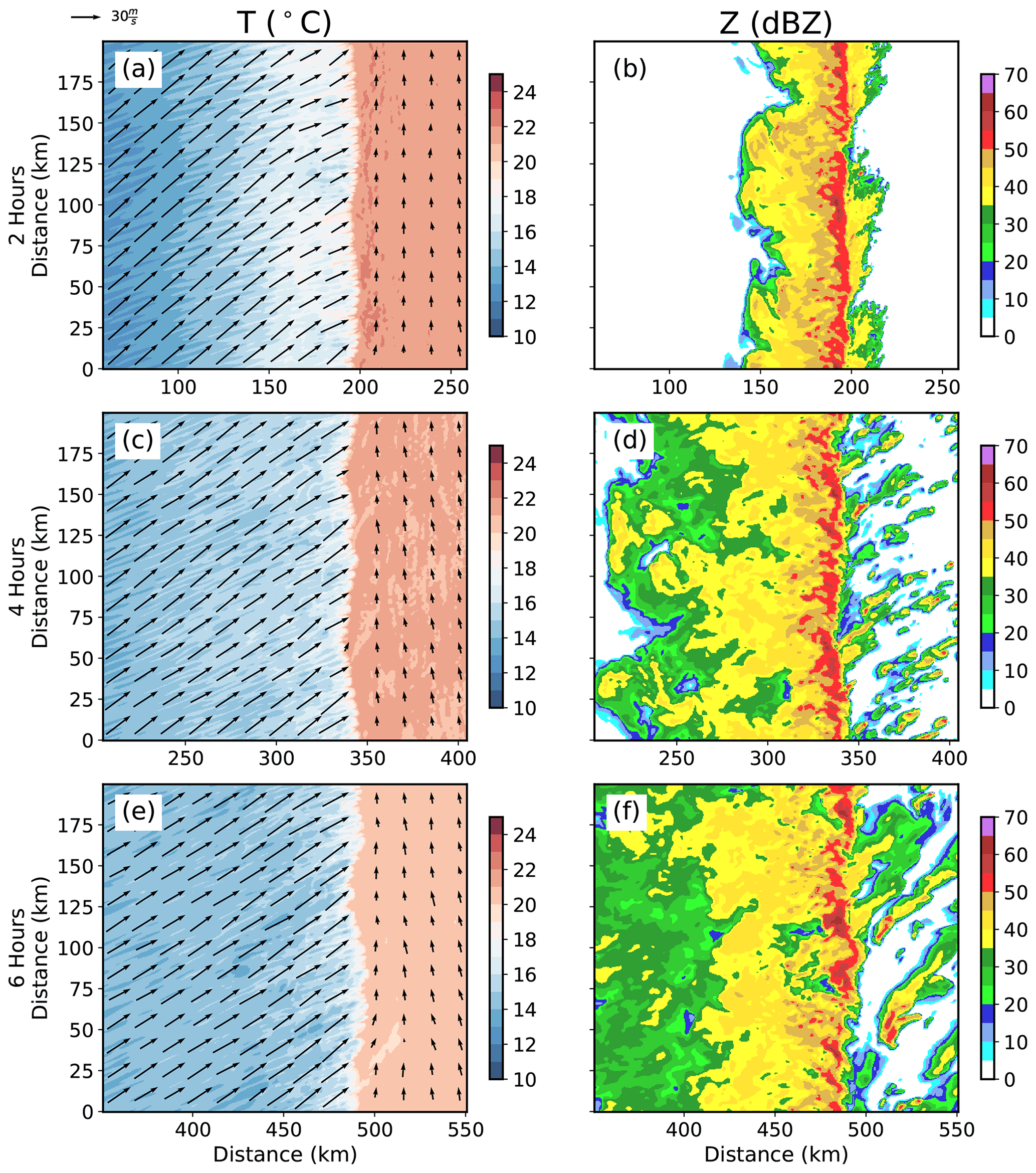
Figure 4Nature run (a, c, e) T and (b, d, f) Z at the lowest model level (5 m a.g.l.). The 500 m a.g.l. winds are superimposed (a, c, e) using arrows.
The QLCS storm structure changes over the simulation period. During the first 2 h of the simulation (e.g., Fig. 4b), the convective line is robust, and storms are spaced closely together so that it is difficult to discern the individual convective cores. As the simulation progresses, the QLCS-embedded storms become more isolated, and the trailing region of the stratiform precipitation expands in areal coverage (Fig. 4d and f). Boundary layer turbulence and QLCS modifications to the environment also cause isolated storms to initiate in the warm sector (Fig. 4f). Strong vertical wind shear and modest instability cause many of the isolated storms to persist until they exit the domain or are absorbed by the approaching QLCS.
Severe weather hazards (e.g., tornadoes, wind, and hail) are small in scale and not fully resolved by the nature run simulation. Since these phenomena cannot be explicitly predicted, diagnostic tools are used to identify areas of intense convection in model output. Updraft helicity, which is the vertical integration of updraft intensity multiplied by vertical vorticity between 2 and 5 km (Kain et al., 2008), is a commonly used proxy for severe weather in CAM forecast experiments (e.g., Kain et al., 2010; Sobash et al., 2011, 2016; Clark et al., 2012; Gallo et al., 2016; Loken et al., 2017; Carlin et al., 2017; Skinner et al., 2018; Potvin et al., 2019; Miller et al., 2022). Updraft helicity can skillfully predict severe weather events because the algorithm identifies mid-level mesocyclones that produce a disproportionately large number of severe weather reports. To identify areas of intense convection and understand how these storms evolve, the nature run maximum updraft helicity is evaluated (Fig. 5).
The nature run produces several long-track swaths of enhanced updraft helicity (>500 m2 s−2), which suggests that some QLCS embedded storms are capable of producing severe weather. QLCS updraft helicity swaths (Fig. 5a) are short-lived and numerous in the western half of the experiment domain, where the storm system initiates and individual storm cells frequently interact (Fig. 4b). Later in the simulation, as the QLCS convective cores become more diffuse (Fig. 4d), the number of updraft helicity swaths decreases (Fig. 5a; 300 km km). In the eastern quarter of the experiment domain (x>400 km), isolated storms initiate ahead of the QLCS and produce long, uninterrupted updraft helicity swaths (Fig. 5c). The rotating storms initially move northeasterly until interacting with the QLCS, after which the updraft helicity intensity decreases and then the swaths rotate eastward. The complex storm interactions for this case highlight the challenges to predict severe weather hazards associated with an evolving QLCS.
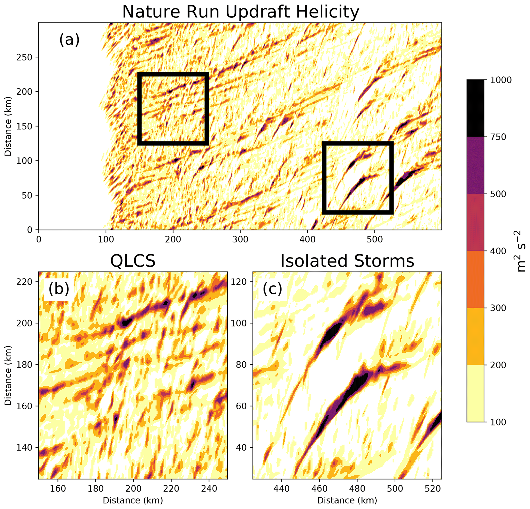
Figure 5Nature run maximum updraft helicity over the (a) full experiment domain. Subdomains plotted in panels (b) and (c) highlight QLCS-embedded mesovortices (left black box) and isolated convection (right black box), respectively.
Rather than using random perturbations to generate the initial ensemble, this study relies on the uncertainties introduced by model physics. The following steps are taken to create each of the 40 ensemble members for this case:
-
Step 1. Initialize two separate, horizontally homogenous simulations with a warm-sector environment (Fig. 1a) and a cold-sector environment (Fig. 1b).
-
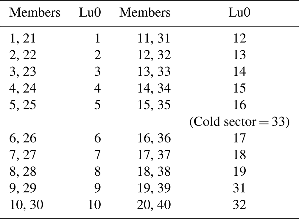
Step 2. Select a model surface type (Table 1) and insert random (±0.25 K) θ perturbations.
-
Step 3. Run both simulations for 24 h, using the ensemble prediction model settings.
-
Step 4. Blend the simulations together to recreate the initial frontal boundary.
The remainder of this section explains, in depth, the procedure used to generate forecast initial conditions.
3.1 Ensemble initialization
Simulations are run with different land surfaces to allow the atmosphere to evolve freely and generate the 40-member forecast ensemble. To avoid spawning the QLCS early, two separate simulations are created for each ensemble member to predict the evolution of the air mass ahead (i.e., warm sector) and behind (i.e., cold sector) the front. The warm-sector simulation is initialized with the nature run initial sounding (Fig. 1a). Perturbations of θ, Td, and u wind consistent with the nature run (−10 K, −20 K, 10 m s−1, respectively) are added to the initial sounding to create the cold-sector environment (Fig. 1b). Perturbation amplitude decreases as a cosine function of height above the surface and extends 6 km a.g.l. Once both simulations are initialized, pseudo-random potential temperature perturbations (±0.25 K) are inserted into the environments to further encourage ensemble diversity.
Parameterized air–surface interactions are a substantial source of forecast uncertainty. Land surface conditions impact the boundary layer and can subsequently alter the evolution of the storm (e.g., Reames and Stensrud, 2017, 2018; Yang et al., 2021). Consequently, the heterogeneous surface makeup of the southeastern United States can modify the environment in countless ways. To incorporate these uncertainties into the ensemble design, cold- and warm-sector simulations for each ensemble member are assigned a land surface type that is commonly observed in the southeast (Table 1). Simulated land surfaces include various degrees of suburban and urban sprawl, croplands, grasslands, forests, bogs, and open bodies of water (assumed in warm-sector simulations only). Both simulations are then integrated for 24 h, using the ensemble prediction model settings (Sect. 3.2), so that surface-dependent momentum, heat, and moisture fluxes can modify the lower troposphere.
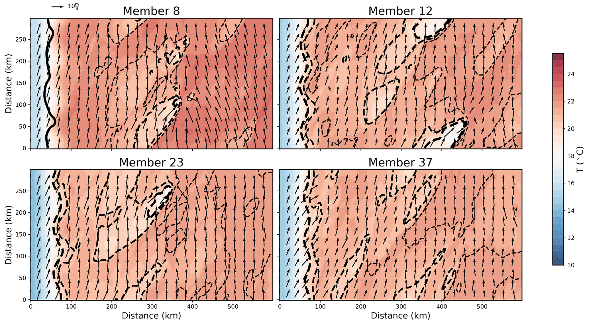
Figure 6Forecast air temperature at the lowest model level (25 m a.g.l.) at the time of ensemble initialization (00:00 UTC). Forecast wind speeds sampled at 500 m a.g.l. are plotted with arrows. The differences between the forecast and nature run temperature are contoured in 1 ∘C increments. Contours that are dashed (solid) indicate where the forecast is cooler (warmer) than the nature run. Contours become thicker as the error increases.
Once the cold- and warm-sector simulations are complete, they are blended together using a cosine weighting function consistent with Eq. (1) to form the initial cold-front boundary that initiates the QLCS. The cold-sector simulation solution is given full weight along the western domain boundary. The warm-sector solution is increasingly favored eastward and given full weighting at all locations east of 100 km. To initiate convection at different times and locations, small changes are made to the frontal boundary width (100±5 km), the number of frontal waves (3±0.5), wave amplitude (10±5 km), and phase (). The initial conditions for each ensemble member (Fig. 6) resemble the nature run; however, given the 24 h spin-up, there is greater uncertainty in environmental conditions.
Table 1The surface types used to generate the initial ensemble of forecasts. Lu0 is the initial land use index in the CM1 namelist.
3.2 Prediction model settings
The forecast ensemble is designed to resemble the National Severe Storms Laboratory's Warn-on-Forecast System (WoFS; Wheatley et al., 2015; Jones et al., 2016) – a frequently updated CAM forecast ensemble that predicts the evolution of severe weather events in real time. This strategic choice allows OSSEs to assess how assimilated observations impact a real-time ensemble prediction system that provides guidance to the operational community (e.g., Wilson et al., 2021; Gallo et al., 2022). Forecasts are run on a numerical mesh with 200×100 points in the x and y directions, respectively, a uniform horizontal spacing of 3 km, and 50 vertical levels. Vertical grid spacing is stretched, with the smallest grid spacing (Δz=50 m) located at the surface, and the coarsest grid spacing (Δz=550 m) located at the 15 km model top. Forecast prediction model settings are identical to those used for the nature run, save for a few notable exceptions. First, the SGS turbulence is disabled in the ensemble forecasts, and the one-dimensional Yonsei University (YSU) planetary boundary layer (PBL) scheme (Hong et al., 2006) is used to parameterize the effects of boundary layer turbulence in the vertical direction. Second, the forecast ensemble and nature run are generated using different versions of the CM1 (release 20.1 for the nature run and release 18 for the ensemble). Differences between prediction model releases and other factors (i.e., model physics configuration and grid spacing) are expected to mitigate the identical-twin problem that can cause overly optimistic OSSE results (e.g., Hoffman and Atlas, 2016).
3.3 Forecast results
The initial forecast ensemble represents some of the complexities observed in real-data cases. Although most data assimilation systems make use of Gaussian prior error approximations, the nonlinear error growth attributed to mesoscale processes often causes forecast errors to become non-Gaussian. Data assimilation systems can produce posterior state estimates under these conditions, but subsequent analyses and forecasts are often suboptimal (e.g., Poterjoy et al., 2017; Robert et al., 2018; Buehner and Jacques, 2020; Poterjoy, 2022). Due to the evolution of mesoscale processes in the warm- and cold-sector environments, forecast errors for this OSSE are non-Gaussian (e.g., Fig. 7) and more realistically challenge the performance of the data assimilation system.
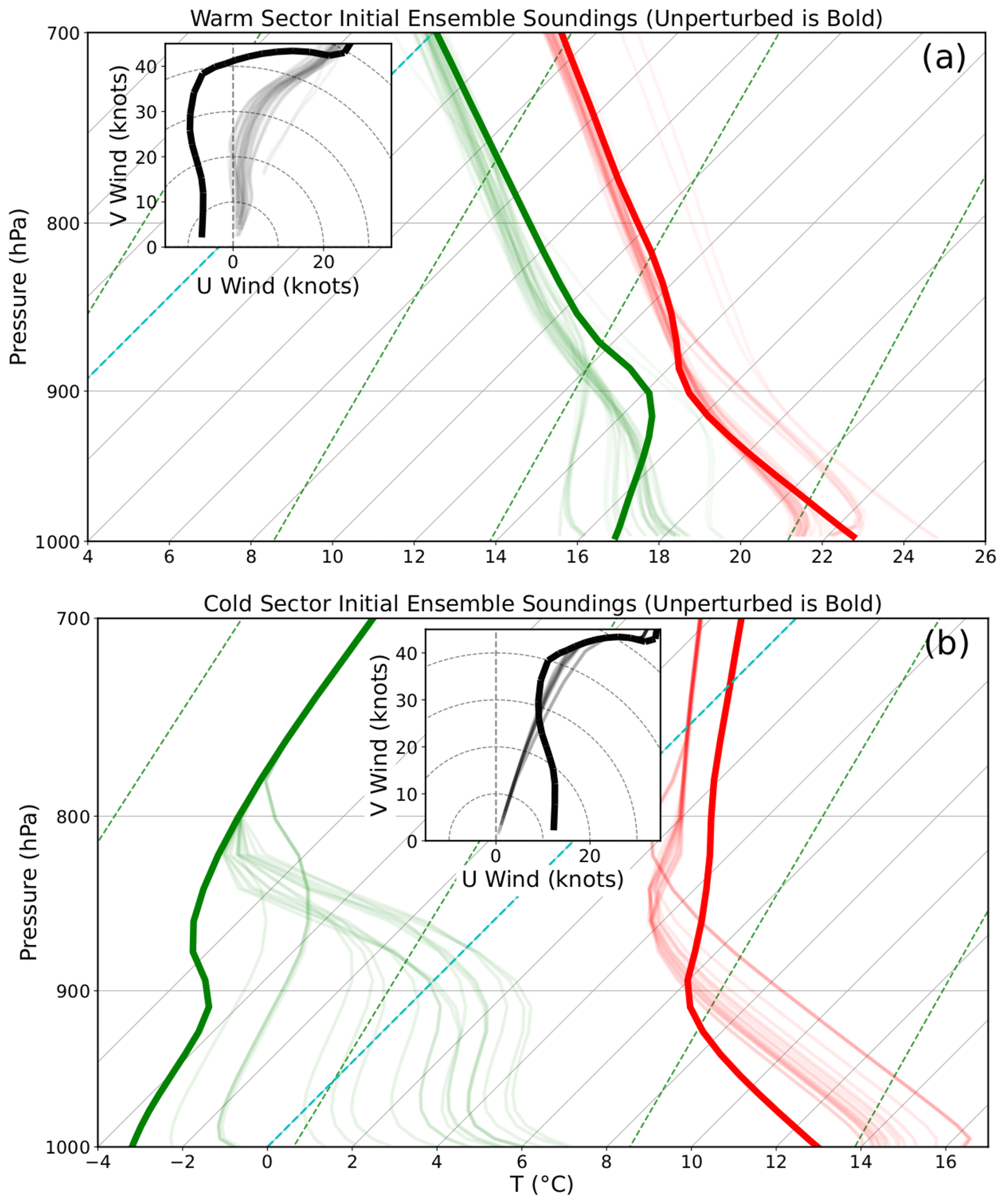
Figure 7Profiles of the domain average (a) warm-sector and (b) cold-sector environments used to generate the initial ensemble. Red, green, and black lines correspond with T (∘C), Td (∘C), and wind (knots). The 40 ensemble member profiles are marked with a thin translucent line. The profiles used to initialize warm-sector and cold-sector simulations (i.e., the unperturbed soundings) are marked by a bold line.
Errors introduced by model physics uncertainties cause the ensemble to drift away from the nature run environment. During the 24 h simulations, storm cold pools and increased cloud cover cause the warm-sector surface layer to moisten and cool on average (Fig. 7a). Relatively warm ground temperatures moisten and heat the lower troposphere in the cold sector (Fig. 7b). Friction also modifies the environment and slows near-surface winds (Fig. 7). Due to the idealized nature of these simulations, there is no pressure gradient force to counteract the impacts of friction, so surface winds are nudged to 0. The ensemble wind spread is larger in the warm-sector simulation (Fig. 7a), in part because convective storms disrupt the environment. Moderating cold- and warm-sector environments causes the atmosphere to become more stable and weakens the frontal intensity (i.e., weaker gradients and less convergence), which impacts the strength of the subsequent forecast QLCS.
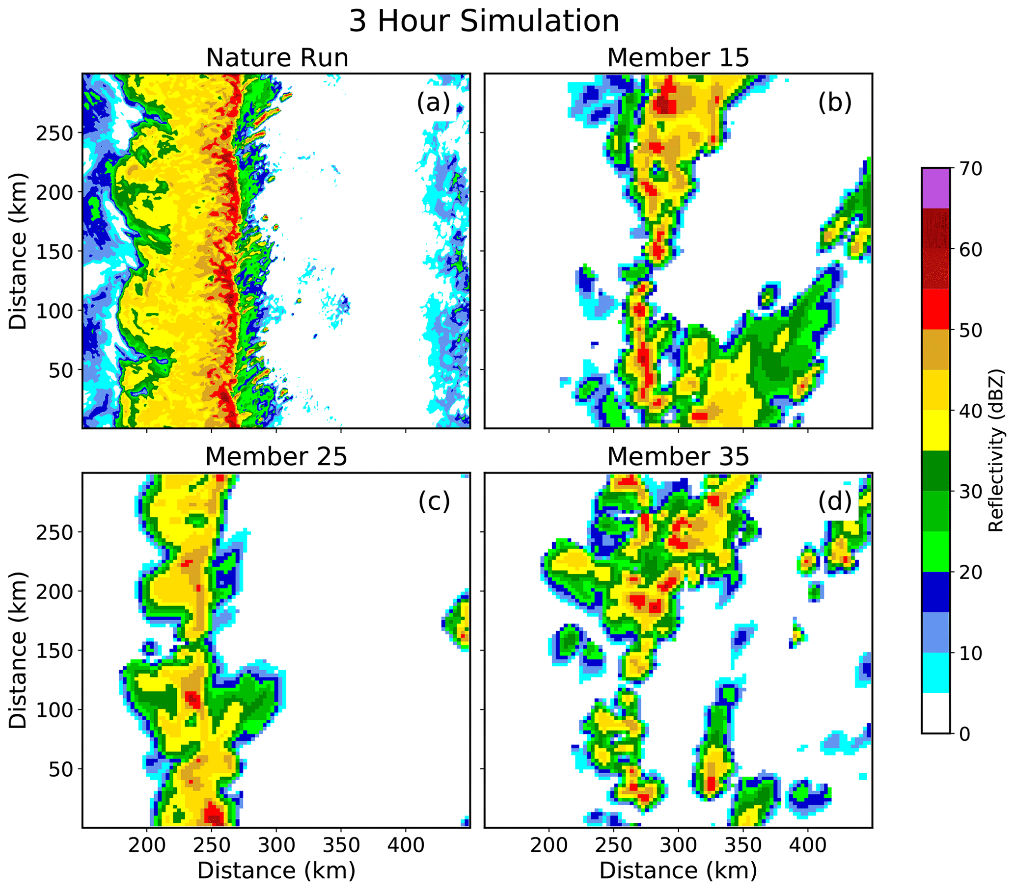
Figure 8(a) Nature run and (b–d) forecast Z at the lowest model level at 03:00 UTC. The forecasts are integrated forward in time without data assimilation.
Modifications to the environment cause forecast storms to be weaker and less numerous than in the nature run simulation (Fig. 8). Some members predict that discrete convective storms will form near the observed QLCS (Fig. 8b and d) but fail to form an organized line of storms. This occurs because moderating warm- and cold-sector environments weakens the frontal boundary temperature gradient. Furthermore, weaker winds diminish the convergence that initiates the line of storms. Some ensemble members predict a QLCS (Fig. 8c), but the storm system is smaller and weaker than in the nature run (Fig. 8a). Differences are attributed to changes in the horizontal grid spacing, which impacts storm updraft intensity and areal coverage (e.g., Bryan et al., 2003; Bryan and Morrison, 2012; Verrelle et al., 2015). Additionally, the environment is more stable and has weaker low-level convergence, so the forecast QLCS is less intense than in the nature run.
The data assimilation configuration for this study is designed to resemble the WoFS (Fig. 9). After initialization, the 40-member ensemble of forecasts undergoes a 30 min spin-up period until 00:30 UTC, when observations are assimilated using the Data Assimilation Research Testbed (DART; Anderson and Collins, 2007; Anderson et al., 2009) ensemble adjustment Kalman filter (EAKF; Anderson, 2001). Observations are assimilated every 15 min over a 2 h window between 00:30–02:30 UTC. Following the data assimilation, the forecast ensemble is run until 07:00 UTC (4.5 h forecast) before the QLCS exits the domain.
Simulated radar, surface, and sounding observations extracted from the nature run simulation are assimilated during this study. Four radar sites that are spaced approximately 240 km apart in the experiment domain (Fig. 10) provide simulated reflectivity (Z) and radial velocity (Vr) observations. The radar observations are interpolated in the vertical direction to generate 14 tilts that are consistent with the next-generation weather radar (NEXRAD; Crum et al., 1993) system scanning pattern. A Cressman (1959) weighting function with a 3 km radius of influence analyzes observations to form a 5 km grid in the horizontal direction. Observations within 150 km of the parent radar site are assimilated. Radar observations update all model state variables, except surface moisture and skin temperature fields.
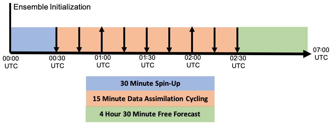
Figure 9The OSSE data assimilation timeline. Downward-pointing arrows indicate times when only radar observations are assimilated. Upward arrows indicate when surface and radar observations are assimilated.
Radar data assimilation alone does not necessarily result in optimal forecast performance due to more realistic and non-Gaussian initial condition errors. This is different from many previous CAM OSSEs that produce skilled forecasts after assimilating only radar observations (e.g., Snyder and Zhang, 2003; Dowell et al., 2004; Caya et al., 2005; Jung et al., 2008; Potvin et al., 2013; Stratman et al., 2018). Conventional observations must also be assimilated in this study to improve the forecast skill. This is consistent with operational forecast systems in which multiple observation sources are always assimilated.
Table 2The data assimilation parameters used for each observation type.
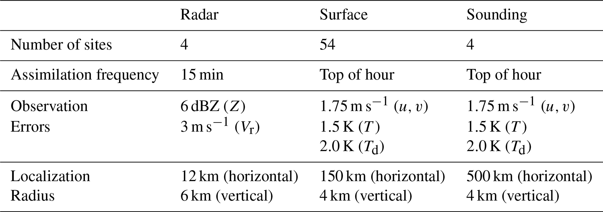
Simulated soundings (i.e., an instantaneous profile of the atmosphere) are assimilated at the top of each hour from each radar site (average site spacing =243.5 km). Soundings sample the atmosphere every 100 m and provide observations of air temperature (T), dew point temperature (Td), and u and v winds. Simulated surface observations mimic what is reported by the automated surface observing system (ASOS) network in real time. Surface observations are assimilated at the top of the hour (Fig. 9) and include 2 m temperature, 2 m dew point temperature, and 10 m u and v winds. The 54 surface stations are randomly distributed throughout the experiment domain to match the approximate spatial density of ASOS stations in the southeastern United States (Fig. 10). Errors are added to each assimilated observation (radar, soundings, and surface) by randomly drawing perturbations from a zero-mean Gaussian distribution that is equivalent to the observation error variance (Table 2).
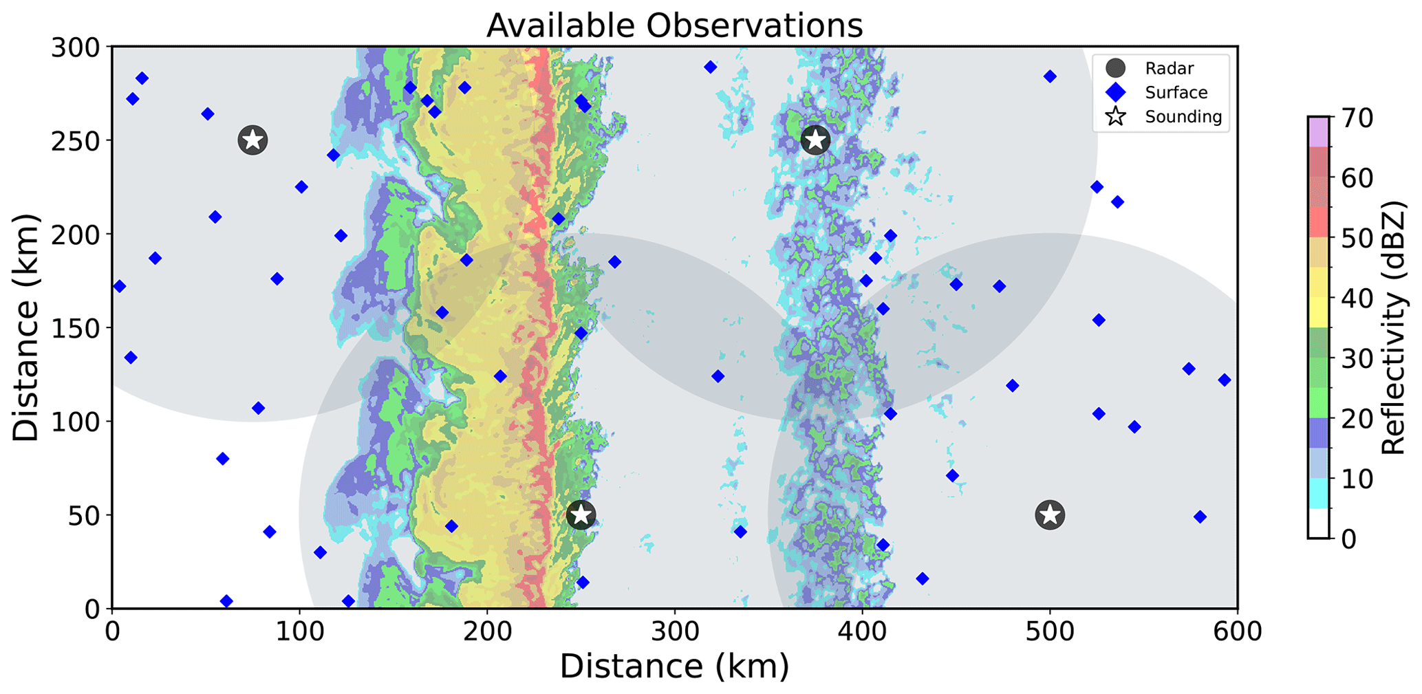
Figure 10The experiment domain with assimilated observations plotted. Large translucent gray circles mark the scanning radius of four radars (marked by the dark circles). White stars mark the sites where soundings are launched. The 54 assimilated surface stations are marked by blue diamonds. Nature run Z at the time of the final data assimilation cycle (02:30 UTC) is plotted for reference.
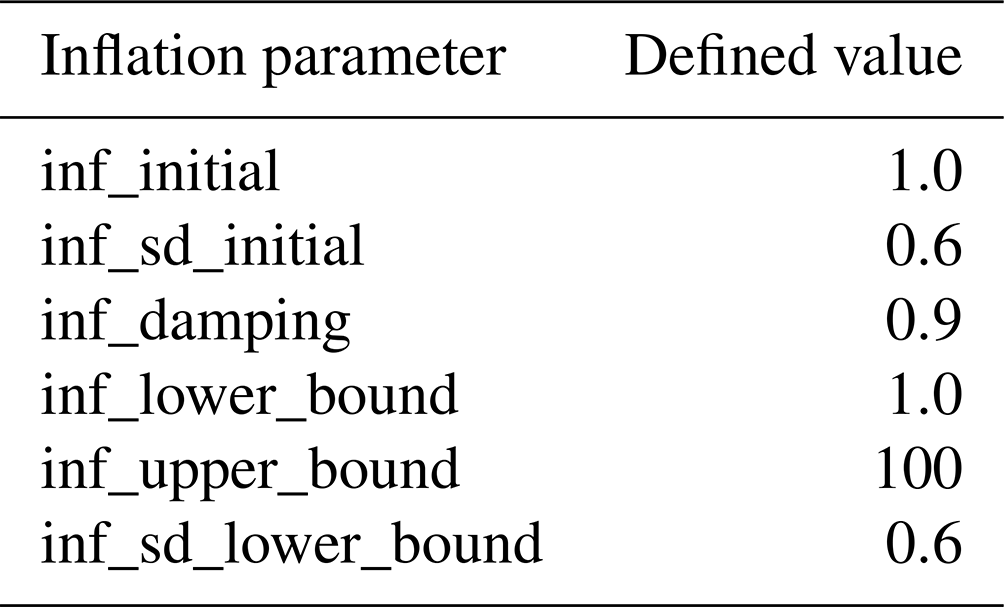
Data assimilation systems are subject to sampling errors that can cause observations to become spuriously correlated with distant model state variables. Left unchecked, the assimilated observations will degrade the analyzed model state and limit the forecast skill. Covariance localization mitigates this problem by limiting the radius over which an assimilated observation can impact the model state. This study uses a distance-based Gaussian weighting function (Gaspari and Cohn, 1999) to limit the range of influence. Localization radii for the assimilated observations closely resemble what is employed by the WoFS (Table 2). Spatially and temporally varying adaptive inflation (Anderson and Collins, 2007) is applied to the prior ensemble to maintain the ensemble spread during data assimilation. Inflation parameters are defined in Table 3.
Table 3The surface types used to generate the initial ensemble of forecasts. Lu0 is the initial land use index in the CM1 namelist.
Observation space statistics provide insight into the data assimilation system performance. The root mean square error (RMSE) quantifies the fit of forecasts and analyses to the observed environment. Rather than calculating statistics at the location of an observing station, errors are calculated for the environmental fields (T, Td, u, and v) over the lowest 3 km of the forecast domain, where the forecast errors are largest. This provides insight into how assimilated observations impact the environment.
Forecast- and nature-run-simulated radar Z sampled at the lowest model level are compared to evaluate the QLCS intensity, position, and structure. The neighborhood maximum ensemble probability (NMEP; Schwartz and Sobash, 2017) of forecast Z exceeding 45 dBZ (P[Z>45 dBZ]) evaluates the storm cores embedded within the QLCS. To mitigate small displacement errors, a 9 km neighborhood is used to generate the probabilistic fields. A Gaussian filter with the same radius smooths the subsequent forecast probabilities. The probabilistic forecast guidance is subjectively compared and objectively verified against the nature run to measure the forecast skill.
The Brier skill score (BSS; Brier, 1950) objectively quantifies the probabilistic forecast skill for this study. This measurement of skill, which ranges between values less than 0 (no skill) and 1 (perfect skill), can be decomposed into reliability, resolution, and uncertainty (Murphy, 1973), as follows:
Reliability is the difference between forecast probability and the relative frequency of the event occurring for that given probability threshold. The forecast skill is optimized when this difference is minimized. The resolution is the difference between the observed climatology of an event occurrence and the frequency at which a forecast event occurs for a given probability threshold. The forecast skill increases with resolution. While the first two parameters are defined by forecast performance, uncertainty is a measure of event climatology. Attribute diagrams, which plot the forecast probability against the observed frequency, provide insight into the forecast reliability and resolution.
Three forecast and data assimilation experiments are run to demonstrate the impact of assimilated environmental and radar observations. The first experiment does not use data assimilation (NoDA), the control experiment (CTRL) assimilates only radar observations, while the final experiment (ENVI) assimilates radar, surface, and sounding observations.
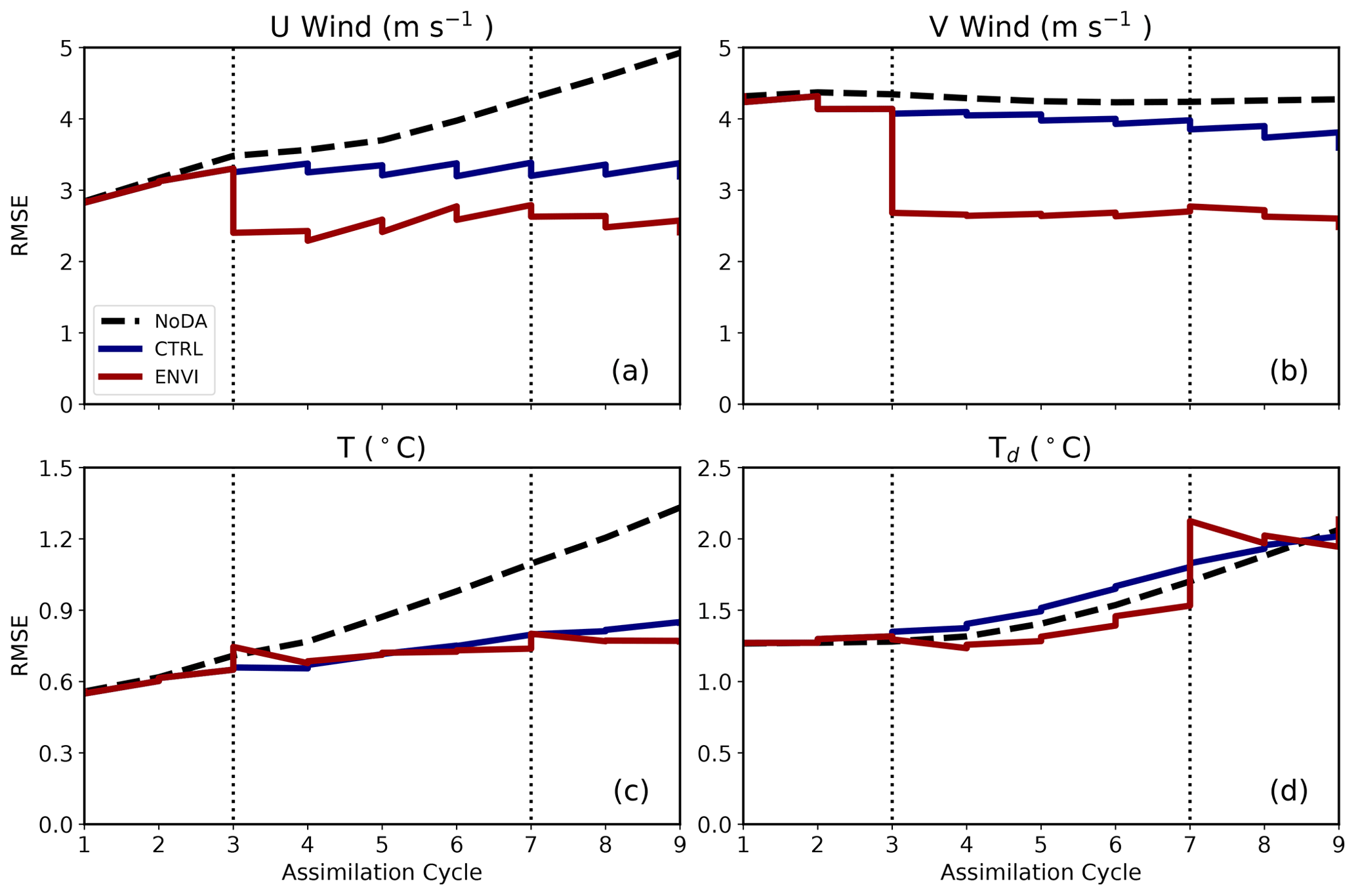
Figure 11The domain-averaged (a) u wind, (b) v wind, (c) T, and (d) Td RMSE during the data assimilation window. Statistics consider the lowest 3 km of the troposphere where forecast errors are largest. Dashed black, solid blue, and solid red lines correspond with NoDA, CTRL, and ENVI, respectively. Vertical dotted lines mark the points when conventional observations (soundings and surface) are assimilated.
The RMSE values (Fig. 11) from the NoDA experiment generally increase over the forecast period. The CTRL RMSE values are relatively improved but remain constant or increase after successive data assimilation cycles. Although cross-covariances allow assimilated radar observations to update the model state, the impact of radar observations is confined to regions near or within convection. Much of the domain is clear air during the data assimilation window (Fig. 10), so radar observations have a limited impact on the broad environment. Assimilated environmental observations substantially reduce the wind field errors (Fig. 11a and b) but have little impact on or increase the T (Fig. 11c) and Td (Fig. 11d) errors. Assimilated sounding observations assume a large localization radius (Table 2) that is consistent with the WoFS configuration. Large localization radii allow atmospheric observations to update large regions of the experiment domain; however, spurious correlations between distant model state variables can potentially increase error. Despite modest increases in error, RMSE values for temperature and moisture fields are comparable between both experiments and remain relatively small (i.e., less than or equal to the observation error variance) throughout the data assimilation window.
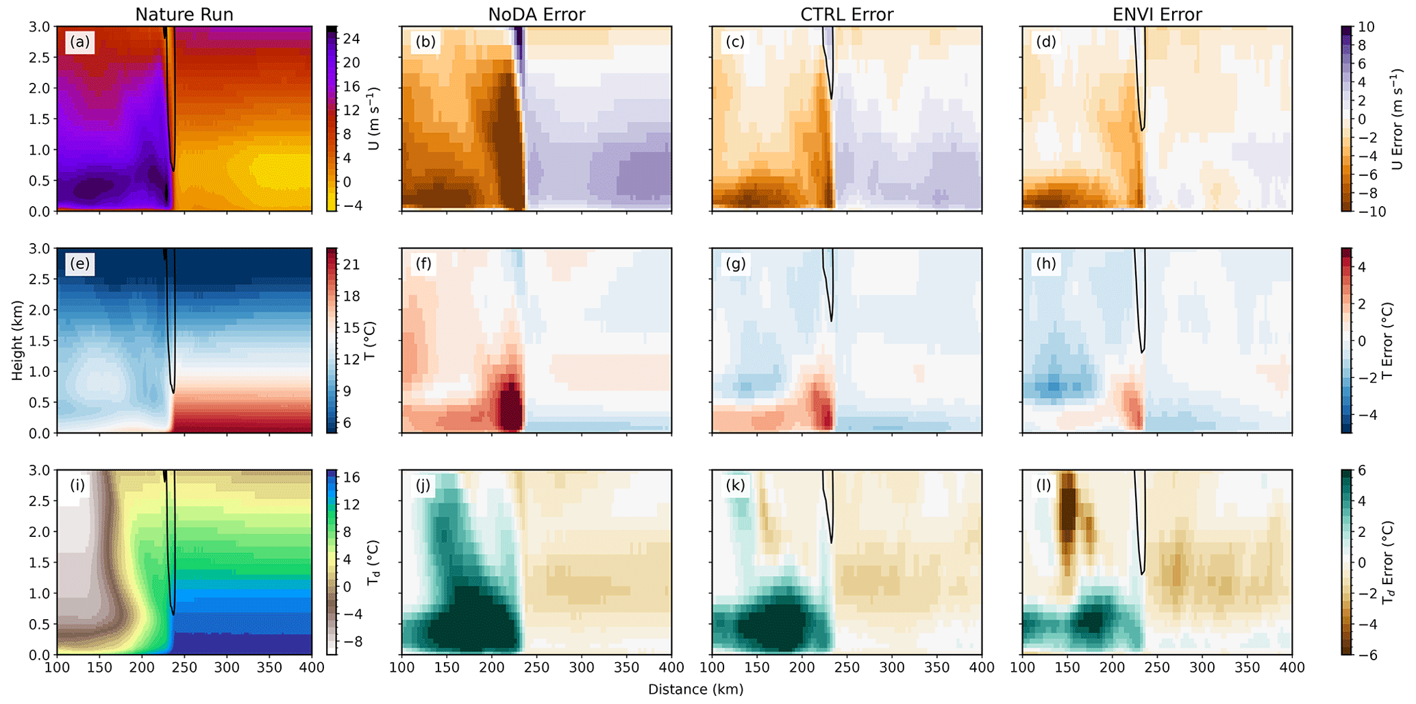
Figure 12Ensemble mean posterior error at the time of the final data assimilation cycle (02:30 UTC) for (b–d) u wind, (f–h) T, and (j–l) Td. Errors are averaged in the north–south direction. Regions where the north–south average updraft velocity exceeds 2.0 m s−1 are contoured.
Assimilated environmental observations enhance frontal boundary wind convergence and cause a more robust QLCS to form. The CTRL posterior u wind field at the final assimilation cycle (Fig. 12c) is positively biased in the lowest 1–2 km of the warm sector (x>250 km). This decreases CTRL frontal convergence because warm-sector winds are directed eastward and away from the QLCS. Assimilated environmental observations decrease ENVI warm-sector wind errors near the surface (Fig. 12d). In the cold sector (x<225 km), ENVI winds are slightly stronger than CTRL, which decreases the error (Fig. 12c and d). This further enhances convergence in ENVI forecasts and provides the mechanical forcing necessary to establish a QLCS that has larger updrafts (Fig. 13). Errors in u wind are largest in the NoDA case for both sectors (Fig. 13b), resulting in greatly reduced convergence and a QLCS with much weaker updrafts (Fig. 13).
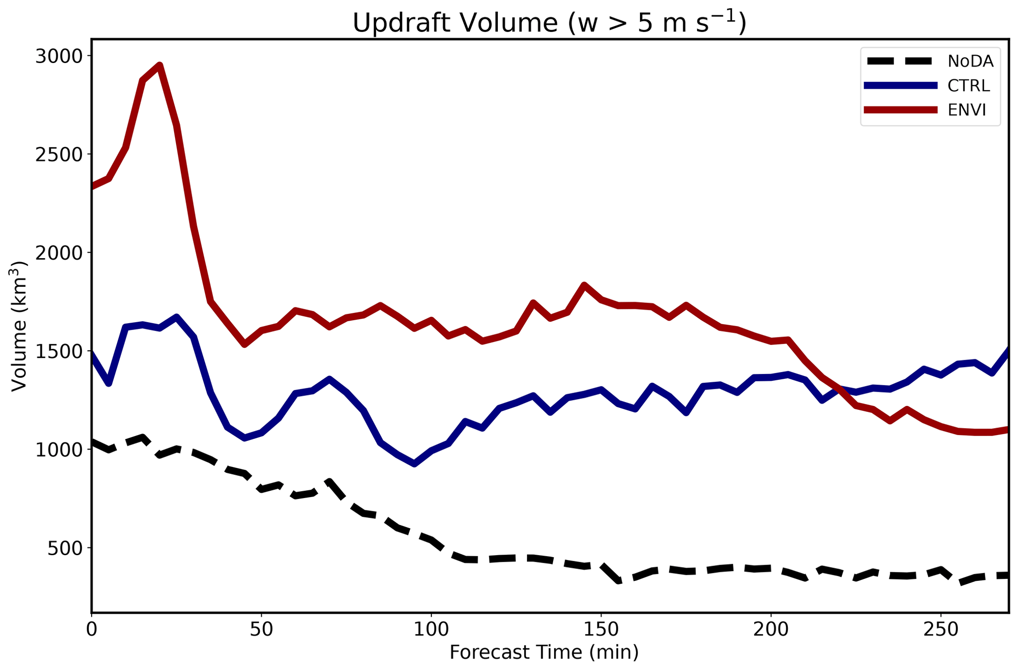
Figure 13Ensemble mean updraft volume during the forecast period. Statistics only consider regions where the updraft velocity exceeds 5 m s−1. Dashed black, solid blue, and solid red lines correspond with NoDA, CTRL, and ENVI, respectively.
While the NoDA experiment again clearly performs the worst, the CTRL and ENVI differences are more subtle for temperature (Fig. 12f–h) and moisture (Fig. 12j–l) fields. All experiments underpredict the cold-sector intensity; the near surface (<0.5 km a.g.l.) is too warm (Fig. 12f–h) and moist (Fig. 12j–l). ENVI cold-sector biases are smaller than CTRL, which suggests that the assimilated environmental observations have a small but positive impact on the posterior state. Analyzed T and Td are similar in the warm sector (x>250 km) for the experiments; ensembles are cool near the surface (Fig. 12f–h) and dry further aloft (>1 km a.g.l.; Fig. 12j–l). Despite localized errors, domain-averaged temperature and moisture errors are relatively small in magnitude (Fig. 11c and d).
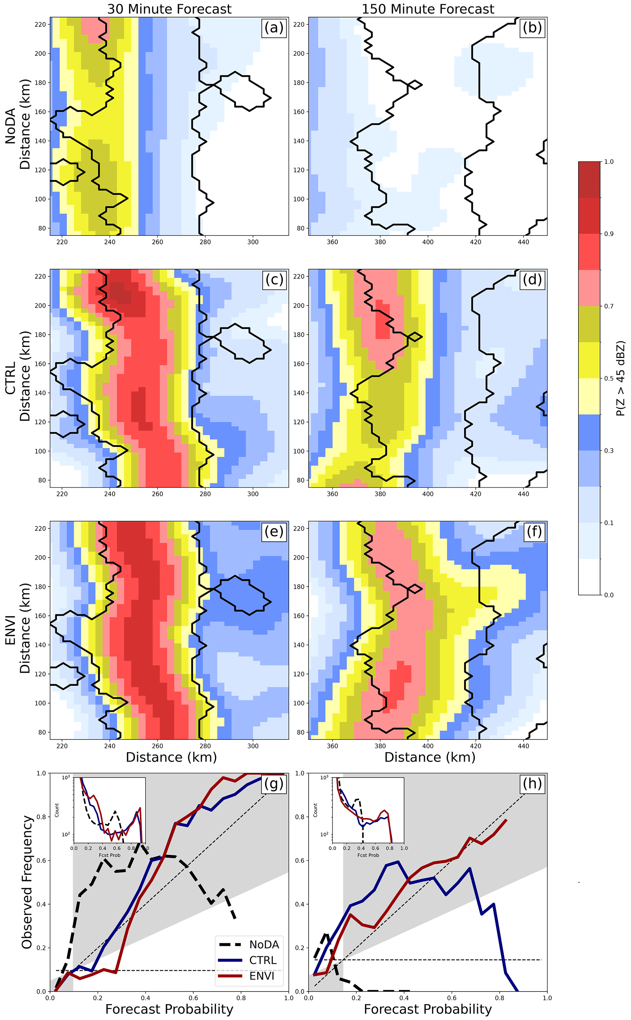
Figure 14The P(Z>45 dBZ) at (a, c, e) 30 and (b, d, f) 150 min for (a, b) NoDA, (c, d) CTRL, and (e, f) ENVI. Regions where the nature run Z exceeds 45 dBZ are contoured black. Attributes diagrams evaluate forecast performance over the full experiment domain at (g) 30 and (h) 150 min.
Assimilated radar observations play an important role in the initial storm placement and intensity (e.g., Snyder and Zhang, 2003). Both the CTRL and ENVI experiments, which assimilate Z and Vr observations, predict high forecast probabilities () to be co-located with observations early in the forecast (Fig. 14c and e), while the same is not true for the NoDA case (Fig. 14a). Consequently, both the CTRL and ENVI experiments have similar attribute curves (Fig. 14g).
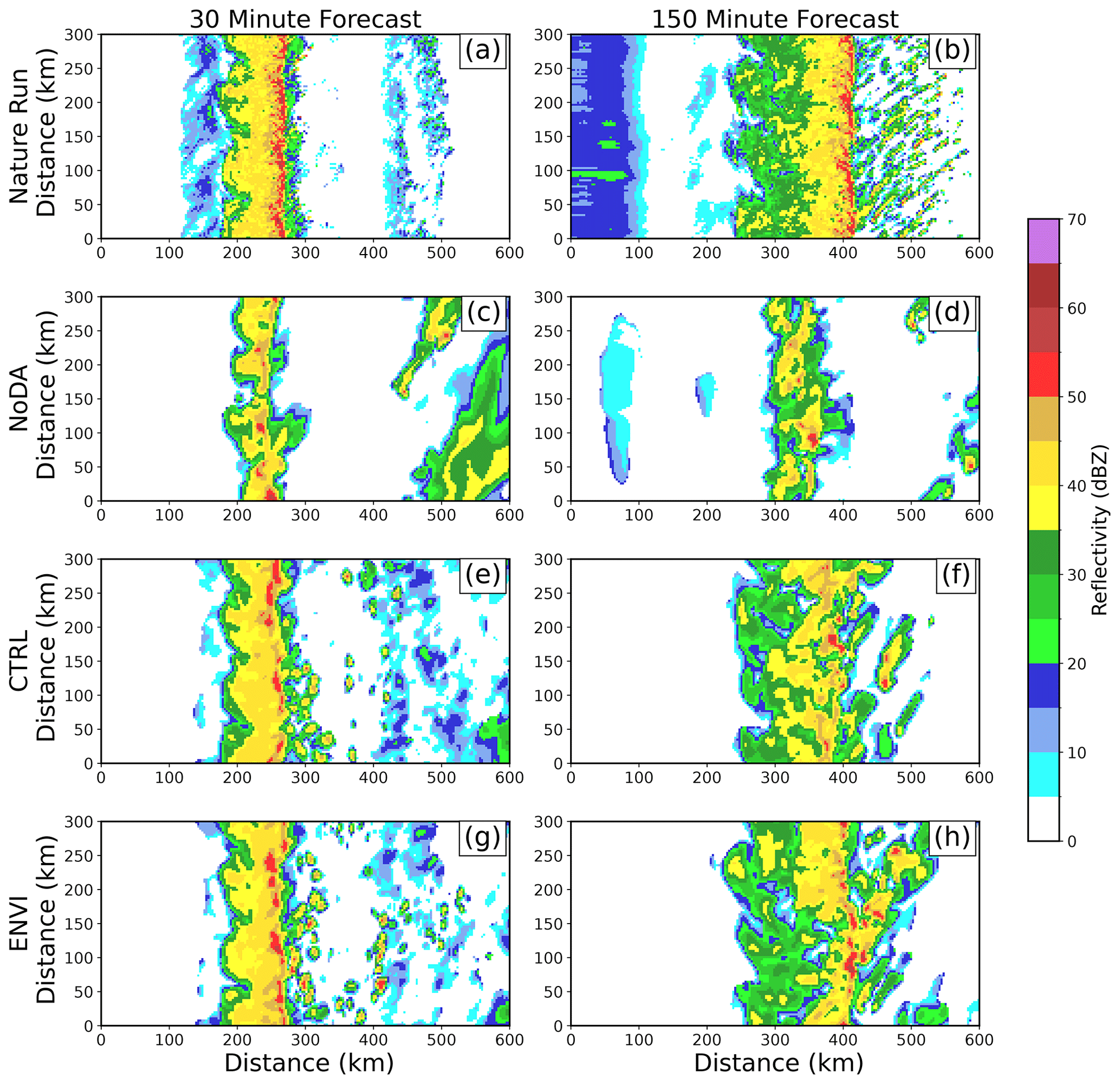
Figure 15(a, b) Nature run and (c–h) forecast (member 25) Z at the lowest model level at (a, c, e, g) 30 and (b, d, f, h) 150 min.
Forecast probabilities become displaced from observations over time (Fig. 14b, d, f). Although individual ensemble members initially resemble the nature run (Fig. 15a, c, e, g), the predicted storms move too slowly during the forecast period (Fig. 15b, d, f, h). Forecast storm motion biases are commonly observed (e.g., VandenBerg et al., 2014) and are sensitive to many factors, including the wind profile errors and cold pool intensity. Due to storm displacement errors, CTRL forecast probabilities far exceed the observed frequency (Fig. 14h) for high-probability thresholds (). The ENVI QLCS moves faster and is more closely located with the observed QLCS, causing the forecast ensemble to become more reliable (Fig. 14h). The areal coverage of high forecast probabilities (; Fig. 14h) is also higher for ENVI than CTRL. Forecast probabilities increase partly because ENVI forecasts predict storm updrafts to be larger than CTRL throughout much of the forecast period (Fig. 13).
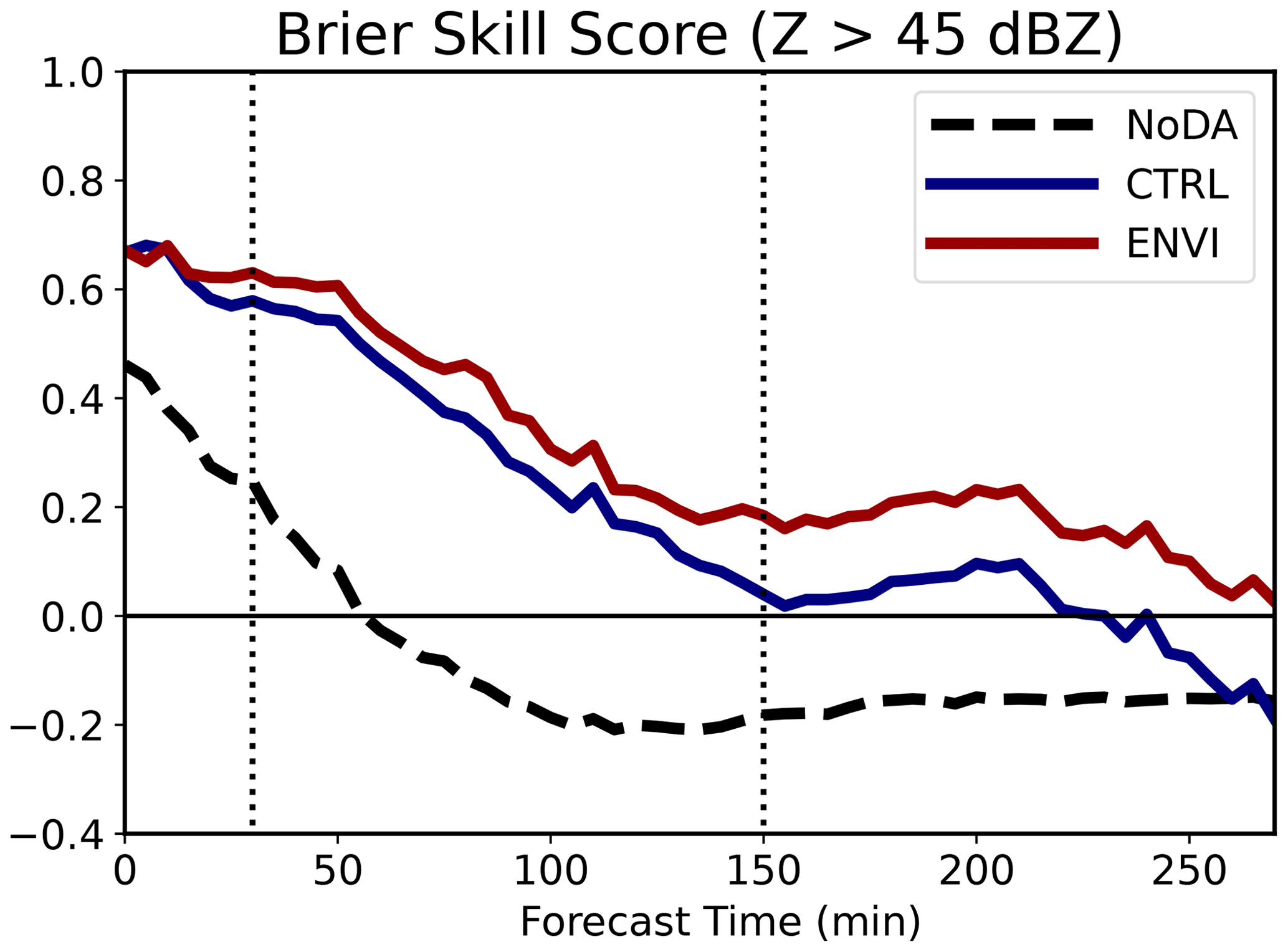
Figure 16The BSS evaluating the P(Z>45 dBZ). Dashed black, solid blue, and solid red lines correspond with NoDA, CTRL, and ENVI, respectively. The horizontal black line marks no skill. Vertical dotted lines mark the times when forecast probabilities are evaluated in Fig. 15.
The NoDA ensemble forecast skill scores are the lowest and reach unity after 1 h (Fig. 16). This is because the forecasts predict the weakest and slowest storm system (e.g., Fig. 15d). Forecast skill scores for both the CTRL and ENVI ensembles are similar early in the forecast period (Fig. 14) but diverge during the first 2 h. The benefits of radar data assimilation wane during this time because small-scale errors quickly grow in scale and impact storm evolution (e.g., Aksoy et al., 2010). For example, CTRL skill decreases faster (Fig. 16) because the predicted QLCS moves too slowly and becomes displaced from observations (Figs. 14d, 15f). The ENVI BSS is higher because the predicted QLCS evolves in an environment that is more representative of the nature run (Fig. 11). Despite these differences, both the CTRL and ENVI ensembles exhibit some skill (BSS >0.0) during the first 4 h of the forecast (Fig. 16). BSSs for both ensembles gradually decrease after this time because the QLCS becomes displaced from observations, the line of storms weakens, and storms ahead of the QLCS fail to initiate with sufficient coverage and intensity.
To gain a more robust understanding of how assimilated observations impact CAM forecast skill, it is imperative that OSSEs include a diverse range of case studies that simulate different storm modes and environments. Unfortunately, the number of idealized case studies for CAM OSSEs is limited. This paper introduces the techniques used to generate a nature run that is representative of a tornadic outbreak in the southeastern United States. The nature run simulates a cold-front boundary that initiates and maintains a QLCS in a highly sheared and modestly unstable turbulent environment. During the 7 h simulation, the QLCS produces multiple mesovortices with isolated rotating thunderstorms that initiate ahead in the warm sector.
This study also introduces a new technique to create an ensemble of forecasts initialized from a single sounding. Uncertainties in the representation of surface conditions are leveraged to create the forecast ensemble. Each forecast member is initialized from the same sounding but runs for 24 h, assuming a different land surface type and small-scale random perturbations. Different surface conditions alter the surface heat, moisture, and momentum fluxes that modify the lower troposphere. The subsequent ensemble is representative of many real-data CAM case studies because the ensemble mean environment is degraded and the initial condition errors are non-Gaussian. This provides the opportunity to understand how assimilated environmental observations will impact forecast skill during a real case study.
The OSSE framework introduced in this study requires a combination of in-storm and environmental observations to create a more skilled QLCS forecast. Forecasts that only assimilate radar observations (reflectivity and radial velocity) predict a relatively weak QLCS that moves too slowly. This is largely because surface friction weakens the initial ensemble wind profile in the lower troposphere which diminishes convergence along the front that initiates and sustains the QLCS. Environmental observations must also be assimilated to correct wind profile errors and increase convergence. Forecasts that assimilate radar and environmental observations (surface and sounding) are consequently more skilled; the QLCS moves faster and has larger updrafts.
The data assimilation experiments conducted in this study are relatively simplistic in their treatment of observations. Environmental observations are interpolated from model output with Gaussian noise to simulate the observation error. This strategy is likely adequate for in situ observations that directly observe the atmosphere (e.g., soundings) but underrepresents retrieved profile errors for remote sensing systems (e.g., Doppler wind lidars and atmospheric emitted radiance inferometers). To better understand the impact of boundary layer profiling systems in future data assimilation experiments, it is imperative to more accurately represent instrument errors. Furthermore, high-resolution modeling studies of the simulated environment are needed to quantify representativeness errors that also introduce uncertainties during data assimilation (e.g., Janjić and Cohn, 2006; Hodyss and Nichols, 2015).
Future work using this OSSE configuration will assimilate different simulated boundary layer profiling instruments to understand their impact on convective initiation and QLCS evolution. Assimilating thermodynamic and kinematic profiles of the boundary layer can improve the representation of the lower troposphere and consequently increase convective initiation forecast skill (e.g., Coniglio et al., 2019; Degelia et al., 2019, 2020; Chipilski et al., 2020). These OSSEs will also help determine an optimal assimilation strategy, including sampling frequency and spatial density. New insights will help determine how these instruments should be deployed during future field campaigns to study and understand high-impact weather in the southeastern United States.
Finally, future studies should develop techniques to quantify the expected level of maximum forecast skill based on event predictability. Understanding the limits of practical predictability (e.g., Melhauser and Zhang, 2012; Zhang et al., 2015; Flora et al., 2018) should help focus the efforts of users looking to optimize the design of, and the assimilation of, observations from new observing networks in the coming decade.
The software and scripts used to generate the initial ensemble forecast, conduct data assimilation, run the free forecast ensemble, and post-process the model output can be found at https://doi.org/10.5281/zenodo.7109050 (Labriola et al., 2022a). In lieu of recreating the data, initial conditions for the nature run, assimilated observations, and the initial prior ensemble at the time of the first assimilation cycle can be accessed at https://doi.org/10.5281/zenodo.7126769 (Labriola et al., 2022b).
JDL created the experiment framework. JDL and JAG conducted the analysis. LJW provided the funding, project administration, and assisted in the project creation and evaluation.
The contact author has declared that none of the authors has any competing interests.
Publisher's note: Copernicus Publications remains neutral with regard to jurisdictional claims in published maps and institutional affiliations.
The authors thank Keith Sherburn and Matthew Parker, who provided the initial sounding and model settings for the QLCS case. Derek Stratman reviewed the journal article prior to submission and provided valuable feedback. Valuable local computing assistance was provided by Gerry Creager, Jesse Butler, and Jeff Horn. Soundings and CAPE calculations are performed with MetPy software.
This research was performed while Jonathan D. Labriola held a National Research Council (NRC) Research Associateship award at the National Severe Storms Laboratory. Funding was provided by the Verification of the Origins of Rotation in Tornadoes Experiment–Southeast (VORTEX-SE) and United States of America (VORTEX-USA) projects.
This paper was edited by Yuefei Zeng and reviewed by two anonymous referees.
Aksoy, A., Dowell, D. C., and Snyder, C.: A multicase comparative assessment of the ensemble Kalman filter for assimilation of radar observations. Part II: Short-range ensemble forecasts, Mon. Weather Rev., 138, 1273–1292, https://doi.org/10.1175/2009MWR3086.1, 2010. a
Anderson, J., Hoar, T., Raeder, K., Liu, H., Collins, N., Torn, R., and Avellano, A.: The Data Assimilation Research Testbed: A Community Facility. B. Am. Meteorol. Soc., 90, 1283–1296, https://doi.org/10.1175/2009BAMS2618.1, 2009. a
Anderson, J. L.: An Ensemble Adjustment Kalman Filter for Data Assimilation, Mon. Weather Rev., 129, 2884–2903, https://doi.org/10.1175/1520-0493(2001)129<2884:AEAKFF>2.0.CO;2, 2001. a
Anderson, J. L. and Collins, N.: Scalable implementations of ensemble filter algorithms for data assimilation, J. Atmos. Ocean. Tech., 24, 1452–1463, https://doi.org/10.1175/JTECH2049.1, 2007. a, b
Brier, G. W.: Verification of forecasts expersses in terms of probaility, Mon. Weather Rev., 78, 1–3, https://doi.org/10.1126/science.27.693.594, 1950. a
Bryan, G. H. and Fritsch, J. M.: A benchmark simulation for moist nonhydrostatic numerical models, Mon. Weather Rev., 130, 2917–2928, https://doi.org/10.1175/1520-0493(2002)130<2917:ABSFMN>2.0.CO;2, 2002. a
Bryan, G. H. and Morrison, H.: Sensitivity of a Simulated Squall Line to Horizontal Resolution and Parameterization of Microphysics, Mon. Weather Rev., 140, 202–225, https://doi.org/10.1175/mwr-d-11-00046.1, 2012. a, b
Bryan, G. H. and Rotunno, R.: Evaluation of an analytical model for the maximum intensity of tropical cyclones, J. Atmos. Sci., 66, 3042–3060, https://doi.org/10.1175/2009JAS3038.1, 2009. a
Bryan, G. H., Wyngaard, J. C., and Fritsch, M. J.: Resolution Requirements for the Simulation of Deep Moist Convection, Mon. Weather Rev., 131, 2394–2416, 2003. a, b
Buehner, M. and Jacques, D.: Non-Gaussian deterministic assimilation of radar-derived precipitation accumulations, Mon. Weather Rev., 148, 783–808, https://doi.org/10.1175/MWR-D-19-0199.1, 2020. a
Carlin, J. T., Gao, J., Snyder, J. C., and Ryzhkov, A. V.: Assimilation of ZDR Columns for Improving the Spin-Up and Forecast of Convective Storms in Storm-Scale Models: Proof-of-Concept Experiments, Mon. Weather Rev., 145, 5033–5057, https://doi.org/10.1175/MWR-D-17-0103.1, 2017. a
Caya, A., Sun, J., and Snyder, C.: A Comparison between the 4DVAR and the Ensemble Kalman Filter Techniques for, Mon. Weather Rev., 133, 3081–3094, 2005. a, b, c, d
Chipilski, H. G., Wang, X., and Parsons, D. B.: Impact of Assimilating PECAN Profilers on the Prediction of Bore-Driven Nocturnal Convection: A Multiscale Forecast Evaluation for the 6 July 2015 Case Study, Mon. Weather Rev., 148, 1147–1175, https://doi.org/10.1175/mwr-d-19-0171.1, 2020. a
Cintineo, R. M. and Stensrud, D. J.: On the predictability of supercell thunderstorm evolution, J. Atmos. Sci., 70, 1993–2011, https://doi.org/10.1175/JAS-D-12-0166.1, 2013. a
Cintineo, R. M., Otkin, J. A., Jones, T. A., Koch, S., and Stensrud, D. J.: Assimilation of synthetic GOES-R ABI infrared brightness temperatures and WSR-88D radar observations in a high-resolution OSSE, Mon. Weather Rev., 144, 3159–3180, https://doi.org/10.1175/MWR-D-15-0366.1, 2016. a
Clark, A. J., Kain, J. S., Marsh, P. T., Correia, J., Xue, M., and Kong, F.: Forecasting Tornado Pathlengths Using a Three-Dimensional Object Identification Algorithm Applied to Convection-Allowing Forecasts, Weather Forecast., 27, 1090–1113, https://doi.org/10.1175/WAF-D-11-00147.1, 2012. a
Cohen, A. E., Cavallo, S. M., Coniglio, M. C., and Brooks, H. E.: A review of planetary boundary layer parameterization schemes and their sensitivity in simulating southeastern U.S. cold season severe weather environments, Weather Forecast., 30, 591–612, https://doi.org/10.1175/WAF-D-14-00105.1, 2015. a
Coniglio, M. C., Correia, J., Marsh, P. T., and Kong, F.: Verification of convection-allowing WRF model forecasts of the planetary boundary layer using sounding observations, Weather Forecast., 28, 842–862, https://doi.org/10.1175/WAF-D-12-00103.1, 2013. a
Coniglio, M. C., Romine, G. S., Turner, D. D., and Torn, R. D.: Impacts of targeted AERI and doppler lidar wind retrievals on short-term forecasts of the initiation and early evolution of thunderstorms, Mon. Weather Rev., 147, 1149–1170, https://doi.org/10.1175/MWR-D-18-0351.1, 2019. a
Cressman, G.: An Operational Objective Analysis System, Mon. Weather Rev., 87, 367–374, 1959. a
Crum, T. D., Alberty, R. L., and Burgess, D. W.: Recording, archiving, and using WSR-88D data, B. Am. Meteorol. Soc., 74, 645–653, https://doi.org/10.1175/1520-0477(1993)074<0645:raauwd>2.0.co;2, 1993. a
Dawson, D. T. I., Wicker, L. J., Mansell, E. R., and Tanamachi, R. L.: Impact of the Environmental Low-Level Wind Profile on Ensemble Forecasts of the 4 May 2007 Greensburg, Kansas, Tornadic Storm and Associated Mesocyclones, Mon. Weather Rev., 140, 696–716, https://doi.org/10.1175/MWR-D-11-00008.1, 2012. a, b
Deardorff, J. W.: Stratocumulus-Capped Mixed Layers Derived From a Three-Dimensional Model, Bound.-Lay. Meteorol., 18, 495–527, https://doi.org/10.1007/BF00119502, 1980. a
Degelia, S. K., Wang, X., and Stensrud, D. J.: An Evaluation of the Impact of Assimilating AERI Retrievals, Kinematic Profilers, Rawinsondes, and Surface Observations on a Forecast of a Nocturnal Convection Initiation Event during the PECAN Field Campaign, Mon. Weather Rev., 147, 2739–2764, https://doi.org/10.1175/mwr-d-18-0423.1, 2019. a
Degelia, S. K., Wang, X., Stensrud, D. J., and Turner, D. D.: Systematic evaluation of the impact of assimilating a network of ground-based remote sensing profilers for forecasts of nocturnal convection initiation during PECAN, Mon. Weather Rev., 148, 4703–4728, https://doi.org/10.1175/MWR-D-20-0118.1, 2020. a
Dowell, D., Wicker, L. J., and Stensrud, D.: High-resolution analyses of the 8 May 2003 Oklahoma City storm. Part II: EnKF data assimilation and forecast experiments, in: 22nd Conf. on Severe Local Storms, 4–8 October 2004, Amer. Meteor. Soc., Hyannis, MA, 2004. a, b, c, d
Dowell, D. C. and Wicker, L. J.: Additive noise for storm-scale ensemble data assimilation, J. Atmos. Ocean. Tech., 26, 911–927, https://doi.org/10.1175/2008JTECHA1156.1, 2009. a
Evensen, G.: Sequential data assimilation with a nonlinear quasi-geostrophic model using Monte Carlo methods to forecast error statistics, J. Geophys. Res., 99, 143–162, 1994. a
Evensen, G.: The Ensemble Kalman Filter : theoretical formulation and practical implementation, Ocean Dynam., 53, 343–367, https://doi.org/10.1007/s10236-003-0036-9, 2003. a
Flora, M. L., Potvin, C. K., and Wicker, L. J.: Practical predictability of supercells: Exploring ensemble forecast sensitivity to initial condition spread, Mon. Weather Rev., 146, 2361–2379, https://doi.org/10.1175/MWR-D-17-0374.1, 2018. a
Flora, M. L., Skinner, P. S., Potvin, C. K., Reinhart, A. E., Jones, T. A., Yussouf, N., and Knopfmeier, K. H.: Object-based verification of short-term, storm-scale probabilistic mesocyclone guidance from an experimentalWarn-on-Forecast system, Weather Forecast., 34, 1721–1739, https://doi.org/10.1175/waf-d-19-0094.1, 2019. a
Gallo, B. T., Clark, A. J., and Dembek, S. R.: Forecasting Tornadoes Using Convection-Permitting Ensembles, Weather Forecast., 31, 273–295, https://doi.org/10.1175/WAF-D-15-0134.1, 2016. a
Gallo, B. T., Wilson, K. A., Choate, J., Knopfmeier, K., Skinner, P., Roberts, B., Heinselman, P., Jirak, I., and Clark, A. J.: Exploring the Watch-to-Warning Space: Experimental Outlook Performance during the 2019 Spring Forecasting Experiment in NOAA's Hazardous Weather Testbed, Weather Forecast., 37, 1–38, https://doi.org/10.1175/WAF-D-21-0171.1, 2022. a
Gallus, W. A., Snook, N. A., and Johnson, E. V.: Spring and summer severe weather reports over the midwest as a function of convective mode: A preliminary study, Weather Forecast., 23, 101–113, https://doi.org/10.1175/2007WAF2006120.1, 2008. a
Gao, J. and Stensrud, D. J.: Some observing system simulation experiments with a hybrid 3DEnVAR system for storm-scale radar data assimilation, Mon. Weather Rev., 142, 3326–3346, https://doi.org/10.1175/MWR-D-14-00025.1, 2014. a
Gaspari, G. and Cohn, S. E.: Construction of correlation functions in two and three dimensions, Q. J. Roy. Meteor. Soc., 125, 723–757, 1999. a
Guyer, J. L. and Dean, A. R.: Tornadoes Within Weak CAPE Environments Across the Continental United States, in: 25th Conference on Severe Local Storms, 11–14 October 2010, Denver, CO, https://ams.confex.com/ams/pdfpapers/175725.pdf (last access: 13 February 2023), 2010. a
Hodyss, D. and Nichols, N.: The error of representation: Basic understanding, Tellus A, 67, 24822, https://doi.org/10.3402/tellusa.v67.24822, 2015. a
Hoffman, R. N. and Atlas, R.: Future observing system simulation experiments, B. Am. Meteorol. Soc., 97, 1601–1616, https://doi.org/10.1175/BAMS-D-15-00200.1, 2016. a
Hong, S. Y., Noh, Y., and Dudhia, J.: A new vertical diffusion package with an explicit treatment of entrainment processes, Mon. Weather Rev., 134, 2318–2341, https://doi.org/10.1175/MWR3199.1, 2006. a
Janjić, T. and Cohn, S. E.: Treatment of observation error due to unresolved scales in atmospheric data assimilation, Mon. Weather Rev., 134, 2900–2915, https://doi.org/10.1175/MWR3229.1, 2006. a
Jiménez, P. A., Dudhia, J., González-Rouco, J. F., Navarro, J., Montávez, J. P., and García-Bustamante, E.: A revised scheme for the WRF surface layer formulation, Mon. Weather Rev., 140, 898–918, https://doi.org/10.1175/MWR-D-11-00056.1, 2012. a
Johnson, A. and Wang, X.: Design and Implementation of a GSI-Based Convection-Allowing Ensemble Data Assimilation and Forecast System for the PECAN Field Experiment. Part I: Optimal Configurations for Nocturnal Convection Prediction Using Retrospective Cases, Weather Forecast., 32, 289–315, https://doi.org/10.1175/waf-d-16-0102.1, 2017. a
Johnson, A., Wang, X., Kong, F., and Xue, M.: Object-based evaluation of the impact of horizontal grid spacing on convection-allowing forecasts, Mon. Weather Rev., 141, 3413–3425, https://doi.org/10.1175/MWR-D-13-00027.1, 2013. a
Jones, T. A., Knopfmeier, K. H., Wheatley, D. M., Creager, G. J., Minnis, P., and Palikonda, R.: Storm-Scale Data Assimilation and Ensemble Forecasting with the NSSL Experimental Warn-on-Forecast System. Part II: Combined Radar and Satellite Data Experiments, Weather Forecast., 31, 297–327, https://doi.org/10.1175/WAF-D-15-0107.1, 2016. a, b
Jung, Y., Xue, M., Zhang, G., and Straka, J. M.: Assimilation of Simulated Polarimetric Radar Data for a Convective Storm Using the Ensemble Kalman Filter. Part I: Observation Operators for Reflectivity and Polarimetric Variables, Mon. Weather Rev., 136, 2228–2245, https://doi.org/10.1175/2007MWR2288.1, 2008. a, b
Jung, Y., Xue, M., Wang. Y., Zhu, K., and Pan, Y.: Tests of a cycled EnKF data assimilation and forecasts for the 10 May 2010 tornado outbreak in the central US domain, in: 25th Conference on Severe and Local Storms, 11–14 October 2010, Amer. Meteor. Soc., Nashville, TN, 2012. a
Kain, J. S., Weiss, S. J., Bright, D. R., Baldwin, M. E., Levit, J. J., Carbin, G. W., Schwartz, C. S., Weisman, M. L., Droegemeier, K. K., Weber, D. B., and Thomas, K. W.: Some Practical Considerations Regarding Horizontal Resolution in the First Generation of Operational Convection-Allowing NWP, Weather Forecast., 23, 931–952, https://doi.org/10.1175/2008WAF2007106.1, 2008. a, b
Kain, J. S., Dembek, S. R., Weiss, S. J., Case, J. L., Levit, J. J., and Sobash, R. A.: Extracting Unique Information from High-Resolution Forecast Models : Monitoring Selected Fields and Phenomena Every Time Step, Weather Forecast., 25, 1536–1542, https://doi.org/10.1175/2010WAF2222430.1, 2010. a
Kalnay, E.: Atmospheric modeling, data assimilation, and predictability, Cambridge University Press, https://doi.org/10.1256/00359000360683511, 2002. a
Kerr, C. A., Stensrud, D. J., and Wang, X.: Assimilation of cloud-top temperature and radar observations of an idealized splitting supercell using an observing system simulation experiment, Mon. Weather Rev., 143, 1018–1034, https://doi.org/10.1175/MWR-D-14-00146.1, 2015. a, b
Labriola, J. D. and Wicker, L. J.: Creating Physically‐Coherent and Spatially‐Correlated Perturbations to Initialize High‐Resolution Ensembles of Simulated Convection, Q. J. Roy. Meteor. Soc., 148, 1–21, https://doi.org/10.1002/qj.4348, 2022. a, b, c, d
Labriola, J., Gibbs, J., and Wicker, L.: A Method for Generating a Quasi-Linear Convective System Suitable for Observing System Simulation Experiments (v1.0.0), Zenodo [code], https://doi.org/10.5281/zenodo.7109050, 2022a. a
Labriola, J., Gibbs, J., and Wicker, L.: A Method for Generating a Quasi-Linear Convective System Suitable for Observing System Simulation Experiments: Dataset (v1.0.0), Zenodo [data set], https://doi.org/10.5281/zenodo.7126769, 2022b. a
Loken, E. D., Clark, A. J., Xue, M., and Kong, F.: Comparison of Next-Day Probabilistic Severe Weather Forecasts from Coarse- and Fine-Resolution CAMs and a Convection-Allowing Ensemble, Weather Forecast., 32, 1403–1421, https://doi.org/10.1175/WAF-D-16-0200.1, 2017. a
Markowski, P. M.: An idealized numerical simulation investigation of the effects of surface drag on the development of near-surface vertical vorticity in supercell thunderstorms, J. Atmos. Sci., 73, 4349–4385, https://doi.org/10.1175/JAS-D-16-0150.1, 2016. a
Markowski, P. M.: What is the intrinsic predictability of tornadic supercell thunderstorms?, Mon. Weather Rev., 148, 3157–3180, https://doi.org/10.1175/MWR-D-20-0076.1, 2020. a, b
Melhauser, C. and Zhang, F.: Practical and intrinsic predictability of severe and convective weather at the mesoscales, J. Atmos. Sci., 69, 3350–3371, https://doi.org/10.1175/JAS-D-11-0315.1, 2012. a
Miller, W. J., Potvin, C. K., Flora, M. L., Gallo, B. T., Wicker, L. J., Jones, T. A., Skinner, P. S., Matilla, B. C., and Knopfmeier, K. H.: Exploring the Usefulness of Downscaling Free Forecasts from the Warn-on-Forecast System, Weather Forecast., 37, 181–203, https://doi.org/10.1175/WAF-D-21-0079.1, 2022. a
Morrison, H., Curry, J. A., Shupe, M. D., and Zuidema, P.: A New Double-Moment Microphysics Parameterization for Application in Cloud and Climate Models. Part II: Single-Column Modeling of Arctic Clouds, J. Atmos. Sci., 62, 1678–1693, https://doi.org/10.1175/JAS3447.1, 2005. a
Morrison, H., Thompson, G., and Tatarskii, V.: Impact of Cloud Microphysics on the Development of Trailing Stratiform Precipitation in a Simulated Squall Line: Comparison of One- and Two-Moment Schemes, Mon. Weather Rev., 137, 991–1007, https://doi.org/10.1175/2008MWR2556.1, 2009. a
Murphy, A. H.: A New Vector Partition of the Probability Score, J. Appl. Meteorol., 12, 595–600, https://doi.org/10.1175/1520-0450(1973)012<0595:ANVPOT>2.0.CO;2, 1973. a
Nowotarski, C. J., Markowski, P. M., Richardson, Y. P., and Bryan, G. H.: Supercell low-level mesocyclones in simulations with a sheared convective boundary layer, Mon. Weather Rev., 143, 272–297, https://doi.org/10.1175/MWR-D-14-00151.1, 2015. a
Poterjoy, J.: Implications of Multivariate Non-Gaussian Data Assimilation for Multi-scale Weather Prediction, Mon. Weather Rev., 150, 1475–1493, https://doi.org/10.1175/mwr-d-21-0228.1, 2022. a
Poterjoy, J., Sobash, R. A., and Anderson, J. L.: Convective-scale data assimilation for the weather research and forecasting model using the local particle filter, Mon. Weather Rev., 145, 1897–1918, https://doi.org/10.1175/MWR-D-16-0298.1, 2017. a
Potvin, C. K. and Wicker, L. J.: Comparison between dual-doppler and enkf storm-scale wind analyses: Observing system simulation experiments with a supercell thunderstorm, Mon. Weather Rev., 140, 3972–3991, https://doi.org/10.1175/MWR-D-12-00044.1, 2012. a
Potvin, C. K., Wicker, L. J., Biggerstaff, M. I., Betten, D., and Shapiro, A.: Comparison between dual-doppler and EnKF storm-scale wind analyses: The 29–30 May 2004 Geary, Oklahoma, supercell thunderstorm, Mon. Weather Rev., 141, 1612–1628, https://doi.org/10.1175/MWR-D-12-00308.1, 2013. a, b
Potvin, C. K., Carley, J. R., Clark, A. J., Wicker, L. J., Skinner, P. S., Reinhart, A. E., Gallo, B. T., Kain, J. S., Romine, G. S., Aligo, E. A., Brewster, K. A., Dowell, D. C., Harris, L. M., Jirak, I. L., Kong, F., Supinie, T. A., Thomas, K. W., Wang, X., Wang, Y., and Xue, M.: Systematic comparison of convection-allowing models during the 2017 NOAA HWT spring forecasting experiment, Weather Forecast., 34, 1395–1416, https://doi.org/10.1175/WAF-D-19-0056.1, 2019. a
Reames, L. J. and Stensrud, D. J.: Sensitivity of simulated urban-atmosphere interactions in Oklahoma city to urban parameterization, J. Appl. Meteorol. Climatol., 56, 1405–1430, https://doi.org/10.1175/JAMC-D-16-0223.1, 2017. a
Reames, L. J. and Stensrud, D. J.: Influence of a great plains urban environment on a simulated supercell, Mon. Weather Rev., 146, 1437–1462, https://doi.org/10.1175/MWR-D-17-0284.1, 2018. a
Robert, S., Leuenberger, D., and Künsch, H. R.: A local ensemble transform Kalman particle filter for convective-scale data assimilation, Q. J. Roy. Meteor. Soc., 144, 1279–1296, https://doi.org/10.1002/qj.3116, 2018. a
Romine, G. S., Schwartz, C. S., Snyder, C., Anderson, J. L., and Weisman, M. L.: Model bias in a continuously cycled assimilation system and its influence on convection-permitting forecasts, Mon. Weather Rev., 141, 1263–1284, https://doi.org/10.1175/MWR-D-12-00112.1, 2013. a, b
Schneider, R. S., Dean, A. R., Weiss, S. J., and Bothwell, P. D.: Analysis of estimated environments for 2004 and 2005 severe convective storm reports, in: 23rd Conf. on Severe Local Storms, p. 3.5, Amer. Meteor. Soc., St. Louis, MO, https://ams.confex.com/ams/23SLS/techprogram/paper_115246.html (last access: 13 February 2023), 2006. a
Schwartz, C. S. and Sobash, R. A.: Generating Probabilistic Forecasts from Convection-Allowing Ensembles Using Neighborhood Approaches: A Review and Recommendations, Mon. Weather Rev., 145, 3397–3418, https://doi.org/10.1175/MWR-D-16-0400.1, 2017. a
Sherburn, K. D. and Parker, M. D.: Climatology and ingredients of significant severe convection in high-shear, low-CAPE environments, Weather Forecast., 29, 854–877, https://doi.org/10.1175/WAF-D-13-00041.1, 2014. a, b
Sherburn, K. D. and Parker, M. D.: The development of severe vortices within simulated high-shear, Low-CAPE convection, Mon. Weather Rev., 147, 2189–2216, https://doi.org/10.1175/MWR-D-18-0246.1, 2019. a, b
Sherburn, K. D., Parker, M. D., King, J. R., and Lackmann, G. M.: Composite environments of severe and nonsevere high-shear, low-CAPE convective events, Weather Forecast., 31, 1899–1927, https://doi.org/10.1175/WAF-D-16-0086.1, 2016. a
Skinner, P. S., Wheatley, D. M., Knopfmeier, K. H., Reinhart, A. E., Choate, J. J., Jones, T. A., Creager, G. J., Dowell, D. C., Alexander, C. R., Ladwig, T. T., Wicker, L. J., Heinselman, P. L., Minnis, P., and Palikonda, R.: Object-based verification of a prototype Warn-on-Forecast system, Weather Forecast., 33, 1225–1250, https://doi.org/10.1175/WAF-D-18-0020.1, 2018. a, b
Snook, N. and Xue, M.: Effects of microphysical drop size distribution on tornadogenesis in supercell thunderstorms, Geophys. Res. Lett., 35, L24803, https://doi.org/10.1029/2008GL035866, 2008. a
Snook, N., Kong, F., Brewster, K. A., Xue, M., Thomas, K. W., Supinie, T. A., Perfater, S., and Albright, B.: Evaluation of Convection-Permitting Precipitation Forecast Products Using WRF, NMMB, and FV3 for the 2016–17 NOAA Hydrometeorology Testbed Flash Flood and Intense Rainfall Experiments, Weather Forecast., 34, 781–804, https://doi.org/10.1175/waf-d-18-0155.1, 2019. a
Snook, N. A., Xue, M., and Jung, Y.: Analysis of a Tornadic Mesoscale Convective Vortex Based on Ensemble Kalman Filter Assimilation of CASA X-Band and WSR-88D Radar Data, Mon. Weather Rev., 139, 3446–3468, https://doi.org/10.1175/MWR-D-10-05053.1, 2011. a
Snyder, C. and Zhang, F.: Assimilation of Simulated Doppler Radar Observations with an Ensemble Kalman Filter, Mon. Weather Rev., 131, 1663–1677, 2003. a, b, c, d, e, f, g, h
Sobash, R. A. and Stensrud, D. J.: The impact of covariance localization for radar data on EnKF analyses of a developing MCS: Observing system simulation experiments, Mon. Weather Rev., 141, 3691–3709, https://doi.org/10.1175/MWR-D-12-00203.1, 2013. a, b
Sobash, R. A., Kain, J. S., Bright, D. R., Dean, A. R., Coniglio, M. C., and Weiss, S. J.: Probabilistic Forecast Guidance for Severe Thunderstorms Based on the Identification of Extreme Phenomena in Convection-Allowing Model Forecasts, Weather Forecast., 26, 714–728, https://doi.org/10.1175/WAF-D-10-05046.1, 2011. a
Sobash, R. A., Schwartz, C. S., Romine, G. S., Fossell, K. R., and Weisman, M. L.: Severe Weather Prediction Using Storm Surrogates from an Ensemble Forecasting System, Weather Forecast., 31, 255–271, https://doi.org/10.1175/WAF-D-15-0138.1, 2016. a, b
Stratman, D. R., Potvin, C. K., and Wicker, L. J.: Correcting storm displacement errors in ensembles using the feature alignment technique (FAT), Mon. Weather Rev., 146, 2125–2145, https://doi.org/10.1175/MWR-D-17-0357.1, 2018. a, b
Tong, M. and Xue, M.: Ensemble Kalman Filter Assimilation of Doppler Radar Data with a Comprssible Nonhydrostatic Model: OSS Experiments, Mon. Weather Rev., 133, 1789–1807, https://doi.org/10.1175/MWR2898.1, 2005. a
VandenBerg, M. A., Coniglio, M. C., Clark, A. J., VandenBerg, M. A., Coniglio, M. C., and Clark, A. J.: Comparison of Next-Day Convection-Allowing Forecasts of Storm motion on 1- and 4-km Grids, Weather Forecast., 29, 878–893, https://doi.org/10.1175/WAF-D-14-00011.1, 2014. a
Verrelle, A., Ricard, D., and Lac, C.: Sensitivity of high-resolution idealized simulations of thunderstorms to horizontal resolution and turbulence parametrization, Q. J. Roy. Meteor. Soc., 141, 433–448, https://doi.org/10.1002/qj.2363, 2015. a
Wheatley, D. M., Knopfmeier, K. H., Jones, T. A., and Creager, G. J.: Storm-Scale Data Assimilation and Ensemble Forecasting with the NSSL Experimental Warn-on-Forecast System. Part I: Radar Data Experiments, Weather Forecast., 30, 1795–1817, https://doi.org/10.1175/WAF-D-15-0043.1, 2015. a, b
Wilson, K. A., Gallo, B. T., Skinner, P., Clark, A., Heinselman, P., and Choate, J. J.: Analysis of End User Access of Warn-on-Forecast Guidance Products during an Experimental Forecasting Task, Weather, Climate, and Society, 859–874, https://doi.org/10.1175/wcas-d-20-0175.1, 2021. a
Xue, M., Tong, M., and Droegemeier, K. K.: An OSSE framework based on the ensemble square root Kalman filter for evaluating the impact of data from radar networks on thunderstorm analysis and forecasting, J. Atmos. Ocean. Tech., 23, 46–66, https://doi.org/10.1175/JTECH1835.1, 2006. a, b
Yang, L., Li, Q., Yuan, H., Niu, Z., and Wang, L.: Impacts of Urban Canopy on Two Convective Storms With Contrasting Synoptic Conditions Over Nanjing, China, J. Geophys. Res.-Atmos., 126, e2020JD034509, https://doi.org/10.1029/2020JD034509, 2021. a
Yussouf, N. and Stensrud, D. J.: Impact of phased-array radar observations over a short assimilation period: Observing system simulation experiments using an ensemble Kalman filter, Mon. Weather Rev., 138, 517–538, https://doi.org/10.1175/2009MWR2925.1, 2010. a
Zeng, Y., Janjić, T., de Lozar, A., Welzbacher, C. A., Blahak, U., and Seifert, A.: Assimilating radar radial wind and reflectivity data in an idealized setup of the COSMO-KENDA system, Atmos. Res., 249, 105282, https://doi.org/10.1016/j.atmosres.2020.105282, 2021. a
Zhang, F., Snyder, C., and Sun, J.: Impacts of Initial Estimate and Observation Availability on Convective-Scale Data Assimilation with an Ensemble Kalman Filter, Mon. Weather Rev., 132, 1238–1253, 2004. a
Zhang, Y., Zhang, F., Stensrud, D. J., and Meng, Z.: Practical predictability of the 20 May 2013 tornadic thunderstorm event in Oklahoma: sensitivity to synoptic timing and topographical influence, Mon. Weather Rev., 143, 2973–2997, https://doi.org/10.1175/MWR-D-14-00394.1, 2015. a
Zhao, J., Gao, J., Jones, T. A., and Hu, J.: Impact of Assimilating High-Resolution Atmospheric Motion Vectors on Convective Scale Short-Term Forecasts: 1. Observing System Simulation Experiment (OSSE), J. Adv. Model. Earth Sy., 13, e2021MS002486, https://doi.org/10.1029/2021MS002484, 2021. a
- Abstract
- Introduction
- Nature run configuration
- Forecast ensemble configuration
- Data assimilation procedure
- Forecast verification
- Forecast and data assimilation experiment
- Summary
- Code and data availability
- Author contributions
- Competing interests
- Disclaimer
- Acknowledgements
- Financial support
- Review statement
- References