the Creative Commons Attribution 4.0 License.
the Creative Commons Attribution 4.0 License.
 | 28 Mar 2023
Development and validation of a global 1∕32° surface-wave–tide–circulation coupled ocean model: FIO-COM32
Bin Xiao
Fangli Qiao
Xunqiang Yin
Guansuo Wang
Shihong Wang
Model resolution and the included physical processes are two of the most important factors that determine the realism or performance of ocean model simulations. In this study, a new global surface-wave–tide–circulation coupled ocean model FIO-COM32 with a resolution of ∘ × ∘ is developed and validated. Promotion of the horizontal resolution from to ∘ leads to significant improvements in the simulations of surface eddy kinetic energy (EKE), the main paths of the Kuroshio and Gulf Stream, and the global tides. We propose the integrated circulation route error (ICRE) as a quantitative criteria to evaluate the simulated main paths of the Kuroshio and Gulf Stream. The non-breaking surface-wave-induced mixing (BV) is proven to still be an important contributor that improves the agreement of the simulated summer mixed-layer depth (MLD) against the Argo observations even with a very high horizontal resolution of ∘. The mean error in the simulated mid-latitude summer MLD is reduced from −4.8 m in the numerical experiment without BV to −0.6 m in the experiment with BV. By including the global tide, the global distributions of internal tide can be explicitly simulated in this new model and are comparable to the satellite observations. Based on Jason-3 along-track sea surface height (SSH), wavenumber spectral slopes of mesoscale ranges and wavenumber frequency analysis show that the unbalanced motions, mainly internal tides and inertia-gravity waves, induced SSH undulation and are a key factor for the substantially improved agreement between model and satellite observations in the low latitudes and low-EKE regions. For the ocean model community, surface waves, tidal currents and ocean general circulations have been separated into different streams for more than half a century. This paper demonstrates that it is time to merge these three streams for a new generation of ocean model development.
- Article
(29097 KB) - Full-text XML
- BibTeX
- EndNote


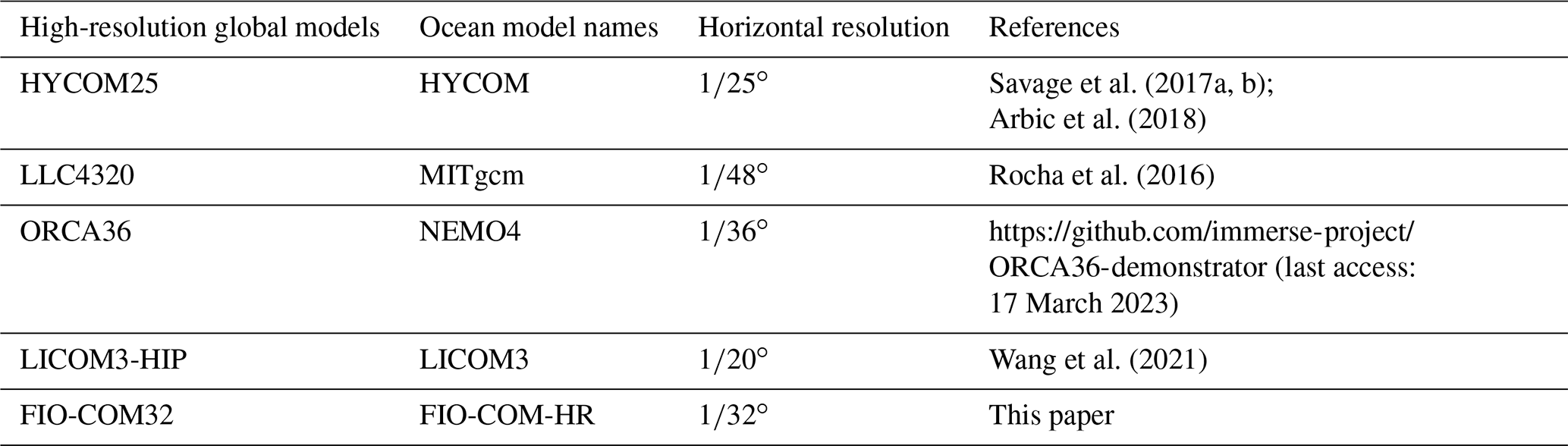
As available computing power has been increasing rapidly, by approximately 1 order of magnitude every 5 years, the state-of-the-art computing ability of modern global ocean numerical models is becoming enormously high, leading to recent achievements in high-resolution global ocean models. The term of “high resolution” as regards present global ocean models may refer to those with horizontal resolutions ranging from 1 to 5 km, which are well beyond the mesoscale resolving threshold in most open oceans (Hallberg, 2013). Further improved resolution has a significant impact on the simulated eddy activities (Thoppil et al., 2011; Sasaki and Klein, 2012; Biri et al., 2016; Ajayi et al., 2020), the vertical mass and buoyancy fluxes (Capet et al., 2016; Su et al., 2018; Dong et al., 2020a), and even the representation of large-scale circulations (Lévy et al., 2010; Chassignet and Xu, 2017). These high-resolution models are not only helpful in improving our scientific understanding of mesoscale and sub-mesoscale eddies and mixed-layer dynamics but are also very useful when evaluating the satellite products of both present (Amores et al., 2018) and future generations, such as SWOT projects (Uchida et al., 2022). Table 1 summarises recent developments in high-resolution global ocean models. Not only is the model horizontal resolution significantly increased, which now ranges from to ∘, but the ocean model physical processes in ocean models are also making notable progresses. For example, HYCOM25 and LLC4320 are global tide–circulation coupled models, and FIO-COM32 is a global surface-wave–tide–circulation coupled ocean model.
Table 1Recent developments in global high-resolution ocean models.
Improving the representation of physical processes in ocean models has been the most fundamental aspect for ocean general circulation model (OGCM) development. Since the establishment of the first OGCM (Bryan and Cox, 1967), surface wave models, tide models, ocean internal wave models and OGCMs have been separated into different streams (Mellor and Blumberg, 2004; Qiao et al., 2004). The most uncertain term in all OGCMs is ocean turbulence. As a result, the vertical structures of ocean temperature and salinity cannot be accurately simulated or predicted. For example, the simulated mixed-layer depth (MLD) in the upper ocean is too shallow, and the sea surface temperature (SST) overheats during summer in nearly all OGCMs. Teixeira and Belcher (2002) investigated the interaction of background turbulence with a monochromatic irrotational surface wave and found that the Stokes drift associated with the surface wave tilts vertical vorticity into the horizontal direction, subsequently stretching it into elongated streamwise vortices, and generates vertical mixing. Qiao et al. (2004, 2016) proposed an upper-ocean mixing scheme of BV induced by surface waves, which plays a dominant role in turbulent mixing of the upper ocean, and analytically expressed BV as a function of the wavenumber spectrum that can be directly calculated from a wave model (Qiao et al., 2004, 2017). Ocean surface wave–circulation coupling has become one of the most important directions of ocean model development. BV has been widely adopted in a series of different OGCMs and climate models, and all models showed dramatic improvements (Qiao et al., 2004; Shu et al., 2011; Song et al., 2012; Fan and Griffies, 2014; Wang et al., 2019). BV is particularly effective in remedying the shallow biases of the simulated MLD and overestimated SST in summer. BV brought the following two surprising results into OGCMs. First, after closing the traditional vertical turbulence schemes, only BV can properly simulates the global ocean, which indicates that BV plays dominant role in vertical mixing in the upper ocean (Qiao and Huang, 2012). Second, BV can cause the MLD to become shallower in winter in climate models, which is also an improvement for climate models (Chen et al., 2018). Although the effect of BV has been comprehensively verified in many coarse-resolution OGCMs, most of these numerical experiments were based on climatological simulations and validated against climatological observations. In order to investigate the impacts of horizontal resolution on the model MLD biases, taking the significantly different behaviours of coarse- and high-resolution models into consideration, it is still necessary to validate the effect of BV in the high-resolution OGCM. For the first time, this paper investigate the BV effects in a high-resolution OGCM of ∘ validated against in situ observations.
Ocean tides have been recognised as a fundamental aspect regulating the hydrodynamic environments in shallow regions (e.g. Simpson and Hunter, 1974; Garrett et al., 1981; Holt and Umlauf, 2008; Lin et al., 2020); thus, ocean tides are often included in regional ocean models. The tidal mixing controls the formation of thermal fronts in coastal regions and generates upwelling (Lü et al., 2006, 2008, 2010). The regional surface-wave–tide–circulation coupled model of the sea around China has shown excellent performance in revealing the three-dimensional circulation structure of Yellow Sea cold water mass (Xia et al., 2006) and has been applied in operational ocean forecasting systems (Wang et al., 2016). In recent years, high-resolution global OGCMs forced by atmospheric forcings begins to include ocean tide explicitly (Arbic et al., 2010, 2012, 2018; Rocha et al., 2016). One of the benefits of including ocean tide in eddy-resolving global OGCMs is that the global distribution of internal tide and mesoscale eddies can be resolved concurrently (e.g. Arbic et al., 2010, 2012, 2018; Buijsman et al., 2015; Shriver et al., 2012; Ansong et al., 2018; Timko et al., 2019). In addition, inclusion of ocean tide in a global ∘ ocean model (MITgcm llc4320) leads to more realistic representation of the unbalanced and ageostrophic motions (Rocha et al., 2016).
To examine whether high-resolution OGCMs can faithfully reproduce the ocean environment, the comparison of wavenumber and frequency spectra against observations is widely adopted (e.g. Sasaki and Klein, 2012; Richman et al., 2012; Chassignet and Xu, 2017, hereafter CX17; Savage et al., 2017a, b; Biri et al., 2016). Therefore, the wavenumber spectral slope in the 70–250 km mesoscale range becomes an important criteria for OGCMs' validation. Sasaki and Klein (2012, hereafter SK12) noted that as the horizontal resolution improved to ∘, the wavenumber spectral slope in the 70–250 km mesoscale range of the model shows quite inconsistent patterns with those of satellite observations. The satellite observations show strong latitudinal variability (Xu and Fu, 2012). In high-latitude and high-eddy-kinetic-energy (EKE) regions, the slopes range between −5 and −4, which is generally consistent with the theory of mesoscale turbulence. However, the slopes are much flatter in tropical and low-EKE regions, which is substantially distinct from the theory of mesoscale turbulence. In high-resolution models such as SK12 and CX17, the slopes range between −5 and −4 in both low- and high-latitude regions. More importantly, Chassignet and Xu (2021, hereafter CX21) showed that as the tide is included in their ∘ Atlantic regional ocean model, the resolved internal tide in sea surface height (SSH) signals is the main explanation for the inconsistency between model and satellite observations. Although ocean tides are included in regional OGCMs, there have still been few attempts to include tides in global OGCMs.
This paper aims to answer the following three key questions through establishing a global ∘ surface-wave–tide–circulation coupled ocean model (FIO-COM32). What are the main effects of increasing horizontal resolution from ∘ to ∘ in a global ocean model? What are the main effects of BV in high-resolution OGCMs? Inspired by the results of an Atlantic regional high-resolution ocean model of CX21, what is the tidal effect in a global ∘ high-resolution OGCM of simulating the wavenumber spectral slopes?
This paper is organised as follows. Section 2 describes the model configurations and design of the numerical experiments. In Sect. 3.1, we present the results of basic aspects of the new global ∘ surface-wave–tide–circulation coupled ocean model and illustrate the effects of increased horizontal resolution by comparing it with a previous global ∘ model. Section 3.2 shows the effects of ocean surface wave and tide coupling in the global ∘ ocean model. Section 4 provides the summary and discussion.
2.1 Model description
FIO-COM consists of a global ocean circulation model, a sea ice model and a global ocean wave model. The ocean circulation component is based on the Modular Ocean Model 5 (Griffies, 2012), the sea ice component is based on the Sea Ice Simulator (Winton, 2000) and the surface wave component is based on the MASNUM (laboratory of MArine Sciences and NUmerical Modelling of the Ministry of Natural Resources of the People's Republic of China) ocean wave model (Yang et al., 2005; Qiao et al., 2017). Currently, the data exchanged between the ocean wave and the ocean circulation model are limited to BV values. The effects of ocean surface currents on surface waves are closed pro tempore to save computer resources and are tested near the end of this paper. BV is calculated in the ocean wave model following Qiao et al. (2004), as in Eq. (1) below, where S(k) represents the wavenumber spectrum and k is the wavenumber. As BV is incorporated into the vertical mixing schemes of the ocean circulation model, α is a tuneable parameter for practical purposes, and we set it as 0.3 in this paper (Wang et al., 2010).
The variable exchanged between the ocean wave and the sea ice models is sea ice concentration (SIC, from the sea ice model to the ocean wave model). The SIC is used to calculate time-varying masks of the ocean wave model, the model domain with SIC exceeding 15 % is masked out as land during the ocean wave model integration.
According to different research purposes, there are two different coupling strategies for the wave model component. Firstly, in the lower-resolution numerical experiments, where the computational costs are not expensive, the wave model component is coupled online with the ocean circulation and sea ice models. The real-time online data exchanges are achieved based on the subroutine version of the MASNUM wave model. In this way, the wave model component could be coupled with ocean circulation and ice components through direct calling of the MASNUM wave model as subroutines in the ocean circulation model. The ocean wave, ocean circulation and sea ice components share the same model grids. Secondly, in the numerical experiments with high computational costs and research focusing on ocean dynamics, the wave component can be turned off to save computational resources (the computational cost of the coupled ocean–ice model is approximately half that of the surface-wave–ocean–ice model). In this configuration, the surface-wave-induced mixing coefficients previously saved in data files are then read into the OGCM; the drawback is that the wave field cannot interact with the ocean circulation fields as they change.
The horizontal grid of FIO-COM32 is a tripolar grid (Murray, 1996) with a horizontal resolution of ∘ × ∘. The model covers the entire global ocean, with a latitudinal coverage of 82∘ S to 90∘ N and a longitudinal coverage of 280∘ W to 80∘ E. Vertically, the z* coordinate (Adcroft and Campin, 2004) is adopted, and the thickness is 2 m at the surface and gradually increases to 367 m at the bottom. The vertical grid has 54 or 57 levels depending on whether ocean tide is introduced. In the numerical experiments without ocean tide, the maximum depth is 5500 m. While the ocean tide is explicitly included, the maximum depth extends to 7000 m by including additional three bottom levels in OGCM. The maximum total grid size is 11 520 × 5504 × 57. Model topography is from GEBCO (IHO-IOC, 2018) and is smoothed by applying a radial filter (Arbic et al., 2004). Model bottom cells are set as partial cells (Adcroft et al., 1997). The horizontal mixing scheme is a bi-harmonic operator with diffusive velocities of 1.96 cm s−1 for momentum and 0.65 cm s−1 for tracers. Both the and ∘ models use the same model settings. The viscosity is calculated from diffusive velocity times the cube of the grid spacing, which means that the viscosity is more than 30 times smaller in the ∘ model than in the ∘ model (FIO-COM10). The vertical mixing scheme uses the K-profile parameterization (KPP) scheme (Large et al., 1994) and BV values. The background vertical viscosity and diffusivity are set as 1.0 × 10⁻⁴ and 3.0 × 10⁻⁵ m2 s−1, respectively. BV is calculated from a global ∘ online coupled FIO-COM model and incorporated into both vertical diffusivity and viscosity. Neither sea surface temperature nor salinity is restored to observational data. The bottom drag is quadratic with a coefficient of 2.5 × 10⁻³.
Ocean tide is explicitly included through introducing eight main tidal generating potentials, i.e. M2, S2, N2, K2, K1, O1, P1 and Q1, in the momentum equations following Schiller and Fiedler (2007). The treatment of self-attraction and loading (SAL) is a simple scalar approximation following Arbic et al. (2010), and the scalar alpha is set to 0.93. The SAL is applied only on the tidal elevations, thus a 25 h running average time filter is adopted to get the slowly varying sea surface height related to large-scale ocean circulation. A topographic drag scheme (Jayne and St. Laurent, 2001) is introduced in the barotropic momentum equation, and this scheme is enabled in the barotropic numerical experiments but closed in the baroclinic experiments because a large portion of the barotropic-to-baroclinic tidal energy conversion can be explicitly resolved in the baroclinic experiments.
The initial conditions, including sea temperature, salinity, velocity and sea surface height (SSH), are interpolated from outcomes of a global operational ocean forecasting system based on FIO-COM10 with a horizontal resolution of ∘ (Qiao et al., 2019; Shi et al., 2018; Sun et al., 2020). As a result, the new ∘ model enters a steady state after a short spin-up period of about 1 year (Fig. A1). The atmospheric forcing is from the Global Forecast System (GFS) of the National Centers for Environmental Prediction (NCEP) (https://www.nco.ncep.noaa.gov/pmb/products/gfs/, last access: 17 March 2023) and has a horizontal resolution of ∘. The ocean surface heat and momentum fluxes are calculated via the bulk formula (Large and Yeager, 2004), and wind stress is calculated using relative wind.
2.2 Numerical experimental design
To investigate to what extent surface waves and tides contribute to the newly established FIO-COM32 model and taking the extremely expensive computational cost into consideration, two numerical experiments are designed. In EXP1, only the OGCM is active, neither the ocean surface waves nor the tides are included, and the simulated period is from 1 June 2016 to 31 December 2019. In EXP2, wave–tide–circulation coupling is enabled, which means both BV and tidal currents are activated. Since the online coupled surface wave model will almost double the computational cost compared with the ocean-only counterpart, in this paper the ∘ numerical experiments uses the BV data calculated from a global ∘ online coupled FIO-COM for the exactly same time period. Here we mainly focus on the effect of BV in the new ∘ ocean model, and due to the large-scale characteristics of the surface wave simulations and the extremely expensive computational costs, we turned off the global ∘ online surface wave model directly and tested the modulation of ocean currents on surface waves near the end of this paper (Fig. 16).
EXP1 starts from outcomes of the global FIO-COM10 forecast system on 1 June 2016. EXP2 branches off from EXP1 on 1 July 2017. The data analysis focuses on the period from 1 January 2018 to 31 December 2019. The model output frequency of three-dimensional variables is daily, and the output frequency of SSH and steric SSH is hourly. An additional two experiments with a horizontal resolution of ∘ are also conducted to investigate the effects of model resolution. The settings of the two ∘ models are kept identical with those of EXP1 and EXP2, respectively; hence, they are named EXP1Low and EXP2Low, respectively. As has been mentioned in the model description, neither sea surface temperature nor salinity is restored to observational data in all of the numerical experiments, and the model drift during the experiment period is examined to ensure that the model maintains a reasonable evolution (Fig. A2). Since the time span of the numerical experiments is not long (3.5 years), the model drift is generally quite small.
Another two numerical experiments, OGCM + BV and OGCM + tide, should be conducted to clearly identify the exact effects of surface waves and tides, respectively. However, considering the high computational costs, we only perform EXP1 and EXP2.
In order to understand how the model resolution affects the simulated barotropic tide, simulation results of the two global barotropic tide models with horizontal resolutions of and ∘ are compared. Ocean temperature and salinity in the global barotropic tide models are set as uniform values and are kept as constants during model integrations. The parameterised topography drag scheme is needed in the barotropic tide models since the energy transfer mechanism from barotropic to baroclinic tide is missing. As has already been noted, a topography drag scheme (Jayne and St. Laurent, 2001) is incorporated into the momentum equation following previous work (Jayne and St. Laurent 2001; Egbert et al., 2004; Arbic et al., 2004), and the drag coefficient is best tuned individually for each numerical experiment. The model topography in this paper is different from our previous work (Xiao et al., 2016) in which the treatment of ice shelf topography of Antarctica is more realistic due to the use of the water column thickness of BEDMAP2 (Fretwell et al., 2013), the use of which would yield a smaller root-mean-square error (RMSE).
3.1 Effects of horizontal resolution
In this section, the surface EKE and SSH values simulated by the ∘ models are compared with those of ∘ models to investigate the sensitivity of different horizontal resolution.
One of the most noteworthy elements of these simulations is that the EKE increases significantly as the model horizontal resolution increases. As CX17 pointed out, this increase is due to smaller effective horizontal viscosity and more active mesoscale and sub-mesoscale motions of higher-resolution models. The simulated surface EKE and satellite observations are compared here to investigate the effects of improved horizontal resolution in FIO-COM32. The surface EKE is calculated as follows:
where u′ and v′ are anomalous zonal and meridional components of surface geostrophic velocity, respectively, which are calculated from sea level anomalies referenced to the mean sea level of 2018 and 2019. The bracket indicates the time averaging of the model years of 2018 and 2019 or the spatial averaging of the global ocean. Satellite-derived surface EKE is calculated using absolute dynamic topography data of Ssalto/Duacs altimeter products produced by the Copernicus Marine and Environment Monitoring service (CMEMS, http://marine.copernicus.eu, last access: 17 March 2023). Generally, increasing the model resolution from to ∘ significantly improves the agreement of the simulated EKE and satellite observations (Fig. 1). Compared with the ∘ model, the ∘ model shows greatly enhanced EKE almost everywhere in the global ocean, especially in the regions of subtropics, mid-latitudes and western boundary current system regions, where surface EKE in the ∘ model is too weak against satellite data. This indicates the horizontal resolution of ∘ is insufficient to properly resolve mesoscale and sub-mesoscale motions, while the simulations of the ∘ model are much improved. For the Kuroshio and Gulf Stream extensions, the EKE amplitudes and spatial distribution structures, such as the separation point and the extension range, are enhanced and agree with the satellite observations much better in the ∘ model. The calculated global mean EKE time series (Fig. 2a) also show improved agreement for the ∘ model against the satellite observations, while the ∘ model has higher global mean EKE values. In order to understand how does the small-scale motions resolved by the ∘ model contribute to the enhanced EKE level, a spatial filter with radius of ∼ 50 km is applied to separate the large-scale (mesoscale or larger) and small-scale (some sub-mesoscale) motions. As a result, the output of SSH of the ∘ model is low-pass filtered, the corresponding low-pass EKE (Fig. 2b) is calculated and the residuals of total EKE are regarded as small-scale contributions (Fig. 2c). Both the low-pass model EKE and CMEMS are on the same ∘ grid, which makes them more comparable. The time series of the low-pass EKE of the ∘ model (the thick solid red line in Fig. 2a) is significantly lower than that of original ∘ model and also lower than that of CMEMS, which indicates the sub-mesoscale motions (such as small-scale eddies and fronts) have important contributions to the enhanced EKE level of the ∘ model (Fig. 2c). On the other hand, the low-pass EKE of the ∘ model is still much more energetic than that of ∘ model. This indicates that the mesoscale eddy fields are more energetic in the ∘ model than in the ∘ model. The calculated RMSE of the 2-year-averaged EKE between model simulations and satellite observations decreases from 63.5 cm2 s−2 in the ∘ model to 31.7 cm2 s−2 in the ∘ model. The RMSE is calculated for regions that have water depths exceeding 1000 m and that are located between 65∘ S and 65∘ N.
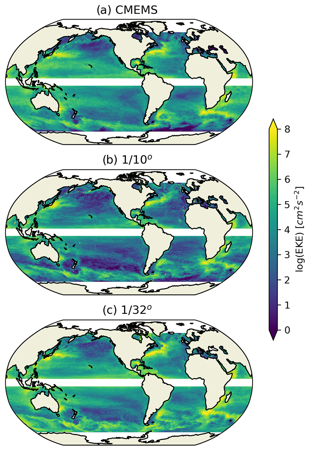
Figure 1Eddy kinetic energy (EKE) of CMEMS from all merged and gridded satellite data (a) and the FIO-COM10 (EXP1Low) (b) and FIO-COM32 (EXP1) (c) model results.
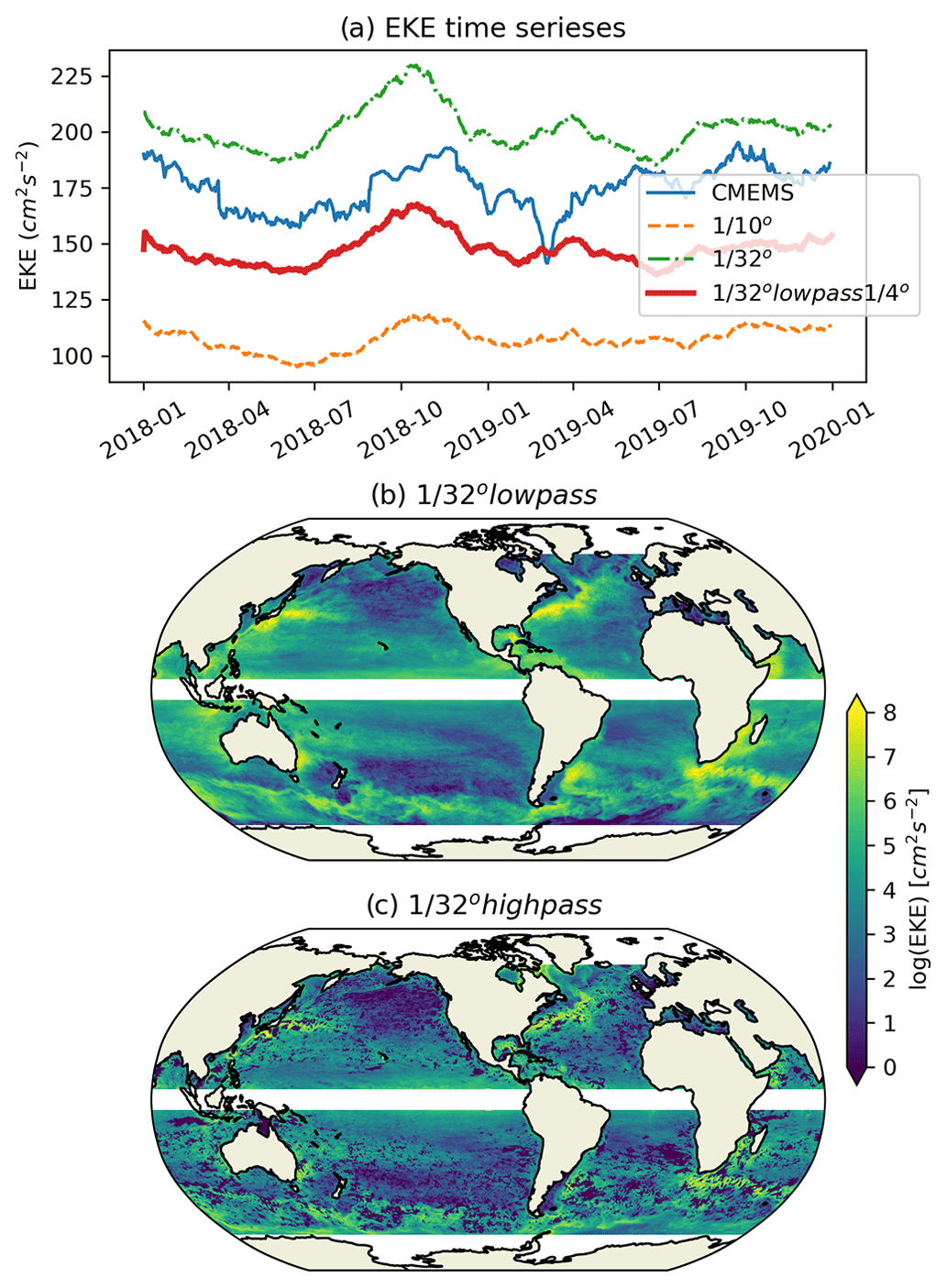
Figure 2Time series of globally averaged EKE (a), EKE of the ∘ model filtered onto a ∘ grid by a low-pass spatial filter with a radius of ∼ 50 km (b) and the EKE residual as a high-pass component (c).
Both the mean SSH and SSH standard deviation (SD) of the and ∘ models are compared in Fig. 3. The large-scale circulation patterns are reasonably simulated in both the and ∘ models (Fig. 3a, c, e). For the detailed simulation structures, such as pathways and separation points of the west boundary currents, the ∘ model shows significant improvements over those of the ∘ model. As the SSH SD comparisons show, the ∘ model is more energetic than the ∘ model in the well-known mesoscale active regions (Fig. 3b, d, f), which has already been discussed in the EKE analysis. In the Kuroshio region, the ∘ model shows over-concentrated energy near the separating point, and the Kuroshio Extension is too weak to penetrate the interior of the Pacific Ocean, but these characteristics are much improved in the ∘ model.
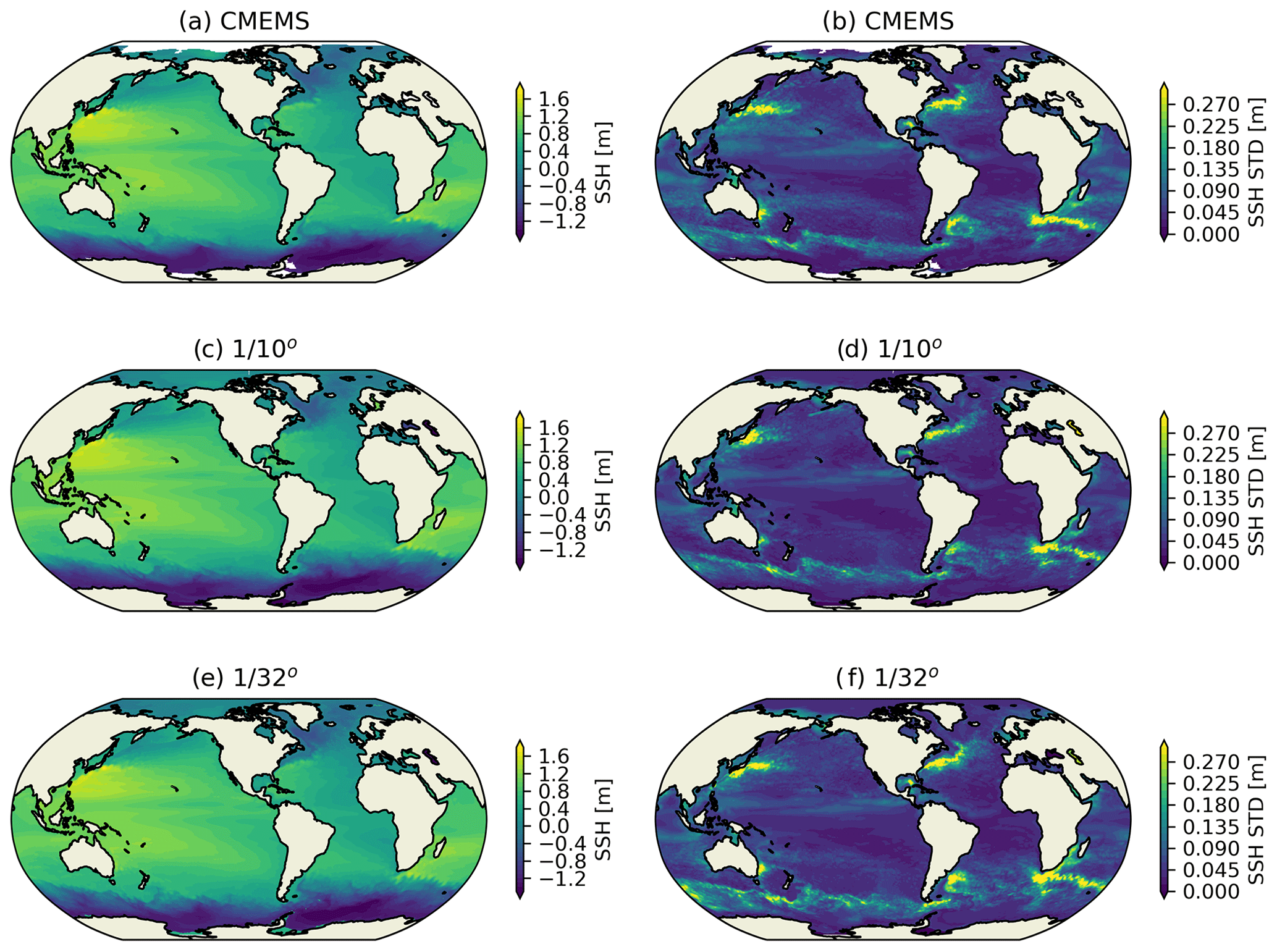
Figure 3Mean SSH (a, c, e) and SSH SD (b, d, f) based on altimeter observations of CMEMS (a, b), FIO-COM10 (c, d) and FIO-COM32 (e, f) simulations.
To better understand the effect of model resolution on the large-scale circulations, we investigated the simulated main paths of the Kuroshio and Gulf Stream. The annual mean SSH of (EXP2Low) and ∘ (EXP2) models of 2019 are compared with the corresponding altimeter observations of CMEMS. In this paper, we propose the integrated circulation route error (ICRE) as a quantitative criteria to assess the quality of the simulated paths of the Kuroshio and Gulf Stream. The ICRE is calculated as follows. First, the path of the western boundary current is defined as the contour edge of SSH at level of 0.16 m. Note that the regionally averaged value is extracted from the SSH before the ICRE analysis is conducted to ensure the SSH of the model and observation are comparable. Second, the ICRE is calculated as the total integrated misfit area between the contour edge of the model and CMEMS, and the regions of the ICRE diagnostics are defined as those in Figs. 4 and 5.

Figure 4Mean SSH of the Kuroshio region. The route of the Kuroshio is represented by the contour line at level of 0.16 m. CMEMS (a), the ∘ model (EXP2Low) (b) and its circulation route errors (d), and the ∘ model (EXP2) (c) and its circulation route errors (e) are shown. Note that the regionally averaged value is extracted from the SSH before the ICRE analysis is conducted to ensure the SSH of the model and observation are comparable.
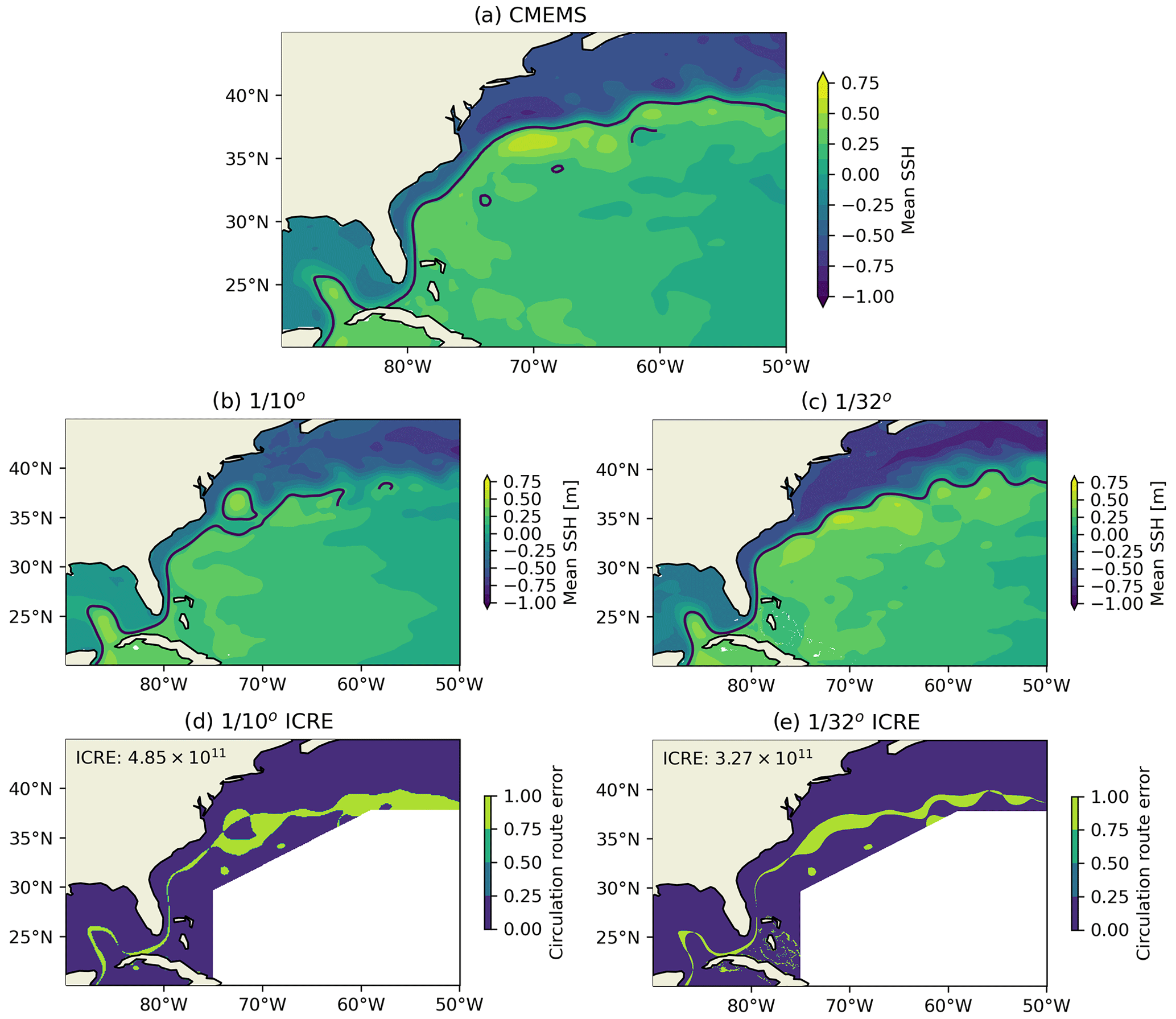
Figure 5The same as Fig. 4 but for the Gulf Stream region. Note that the ICRE of the Gulf stream recirculation is masked out to focus on the main path of Gulf Stream.
As the resolution increases from to ∘, the simulated Kuroshio path is significantly improved (Fig. 4), the ICRE is decreased from 3.01 × 10¹¹ to 1.73 × 10¹¹ m2. The most notable improvement is that the ∘ model is able to reproduce the Kuroshio's large meanders, while the ∘ model cannot. The ICRE of the Gulf Stream is decreased from 4.85 × 10¹¹ m2 in the ∘ model to 3.27 × 10¹¹ m2 in the ∘ model. We should note that for the comparisons of the Gulf Stream region, the recirculation part of the ICRE is masked out to focus on the simulation of main path of the Gulf Stream. Compared to the ∘ model, the ∘ model is not able to reproduce the deep penetration of the Gulf Stream into the Atlantic Ocean (Fig. 5).
Figures 6 and 7 show the simulated relative vorticity of sea surface current in the and ∘ models. They clearly show that as the horizontal resolution increases, the model can resolve many more sub-mesoscale and mesoscale motions. The ∘ model also clearly shows more significant seasonal variations over the ∘ model. This is because the mixed-layer instabilities are substantially enhanced in the ∘ model, especially during winter; this phenomenon is consistent with previous publications (e.g. Sasaki et al., 2017; CX17; Dong et al., 2020b). In the higher-resolution model, the small-scale eddy activities are greatly enhanced during winter compared to those of summer, while this is not as obvious in ∘ model. Stokes drift is the main mechanism that “selectively amplifies the vertical vorticity component as streamwise vorticity” according to Teixeira and Belcher (2002). Since the horizontal scales of the resolved fronts become much smaller in ∘ model, the potential effects of explicit Stokes shear force can be estimated and compared among the models with different horizontal resolutions. The estimation is based on the parameter ϵ proposed by McWilliams and Fox-Kemper (2013):
where Vs is the Stokes drift characteristic velocity; f is the Coriolis parameter; H and L are the depth and width of the front, respectively; and Hs is the Stokes drift decay depth. The estimation is made for a typical section in the Kuroshio Extension region, which is marked as a black line in Fig. 6a. Figures A3 and A4 show the evolution of relative vorticity and temperature along a typical section in the Kuroshio Extension region. The typical horizontal scale of resolved fronts in the ∘ model is about 60 km, while the horizontal scale in the ∘ model is about 3 times smaller (∼ 20 km). The vertical scales of the resolved fronts of both the model and the ∘ model are quite similar, the summer (winter) has a vertical scale of about 30 m (300 m). The dimensionless parameter representing the wave parameters in ϵ is , which is typically O(10–100) (Suzuki et al., 2016). The major difference in the estimations between the and ∘ models is the frontal aspect ratio in ϵ, which is . During summer, the frontal aspect ratio is estimated to be ∼ and ∼ in the and ∘ models, respectively, which yield an estimated ϵ of ∼ and ∼ , respectively. During winter the frontal aspect ratio is estimated to be ∼ and ∼ in the and ∘ models, respectively, yielding an estimated ϵ of ∼ and ∼ , respectively. Hence, it can be concluded that as the horizontal resolution increased from to ∘, the critical resolution may be reached that the explicit Stokes shear force is not to be neglected (at least during winter). In this paper, the BV value is included and could be treated as a “bulk” mixing term accounting for these wave–turbulence interactions. The effect of the explicit implementation of surface-wave-induced forces in the ∘ model remains to be explored in the future.
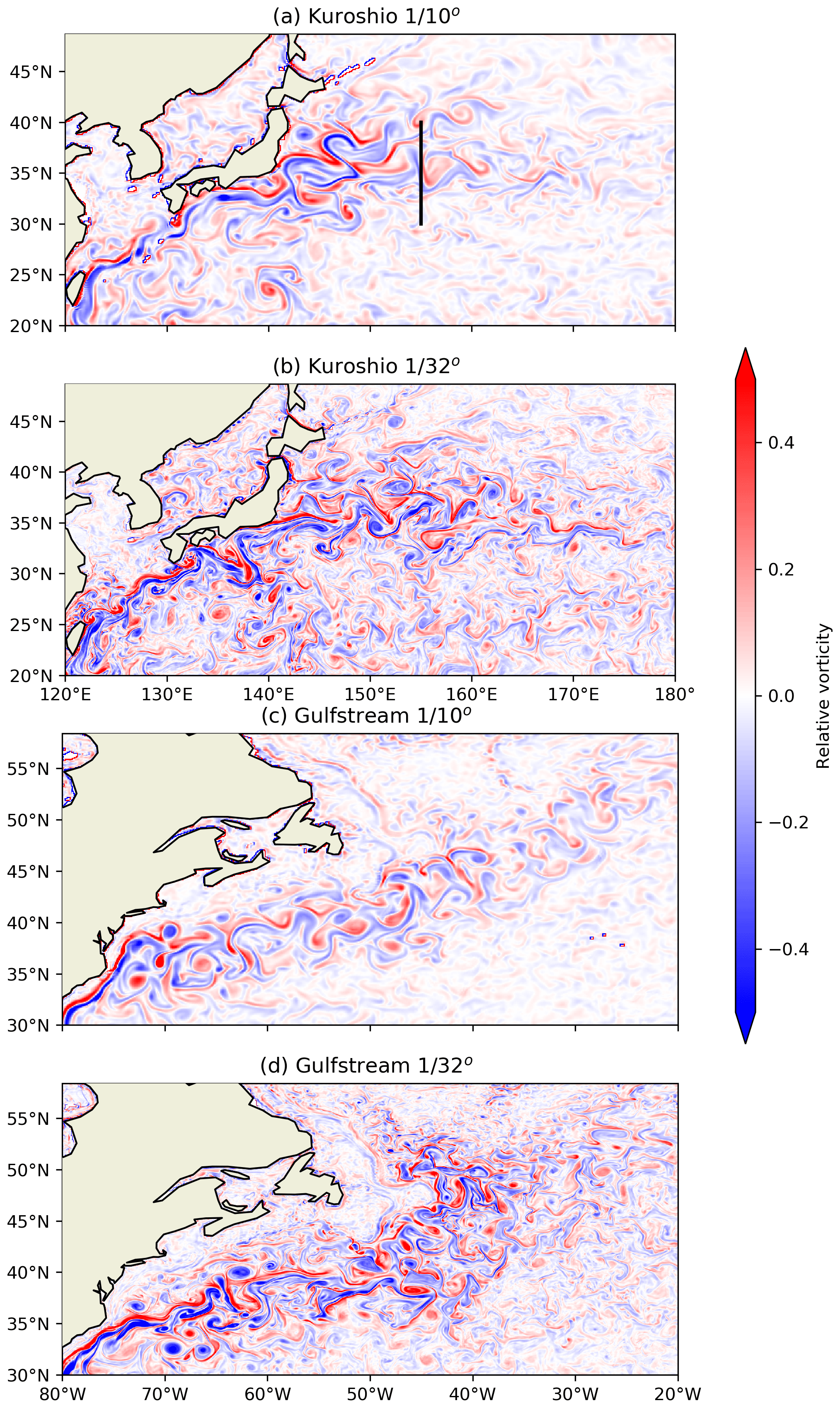
Figure 6Relative vorticity () of the sea surface current in the (a, c) and ∘ (b, d) model results. Snapshots of summer (1 September 2019) of the Kuroshio region (a, b) and the Gulf Stream region (c, d).
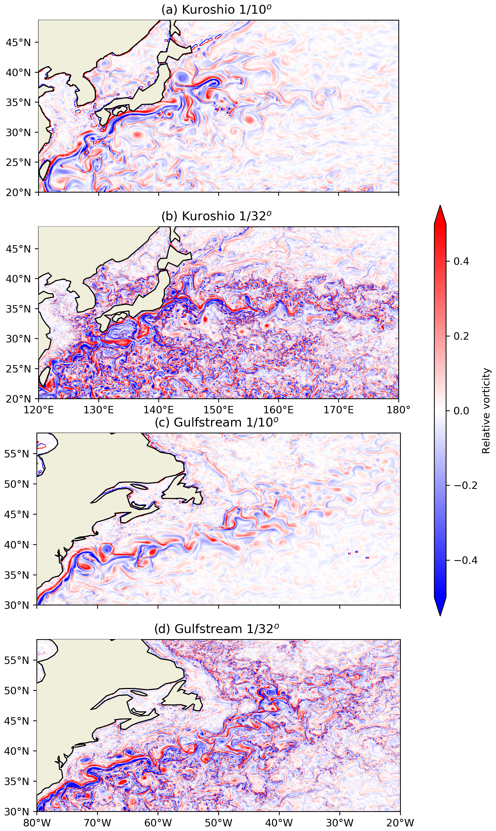
Figure 7The same as Fig. 6 but for winter (1 March 2019).
Reasonable global tide simulation is an important prerequisite for tides and OGCMs to be able to be coupled, since tuning global barotropic tide can also yield better model topography settings, especially as some numerically unstable topography features can be fixed through this practice. The accuracy of simulated global barotropic tide is quite sensitive to the model resolution (Egbert et al., 2004). Here we show the effects of improving horizontal resolutions from to ∘ in the global barotropic tide simulations of FIO-COM. We also present the simulated global tide in EXP2, which is a global baroclinic tide model.
For the ∘ barotropic model, the tidal amplitude is smaller than TPXO9 in some regions, such as west of Panama and in the northeastern Pacific, while the tidal amplitude is stronger than TPXO9 in the Labrador Sea, Sea of Okhotsk and Andaman Sea (Fig. 8b, c). These biases are obviously reduced in the ∘ barotropic model (Fig. 8d), which indicates that the tidal dissipation in the regions of complex terrain is resolved better as the horizontal resolution is increased. The RMSE distributions show that the tidal accuracy of the ∘ barotropic tide model is improved almost everywhere over that of the ∘ barotropic model (Fig. 8e). The statistics show that for the M2 constituent, the globally averaged RMSE of tidal elevation is decreased from 9.65 to 8.06 cm, i.e. reduced by 16.4 %. Here, the tidal elevation RMSE is calculated for regions with water depth exceeding 1000 m and located between 65∘ S and 65∘ N following previous publications (Arbic et al., 2004; Egbert et al., 2004).

Figure 8M2 co-tidal charts of TPXO9 (a), barotropic tide models of ∘ (b) and ∘ (d) resolution with best-tuned topographic drag parameterisation, a baroclinic tide model of ∘ resolution (EXP2) (f) without topographic drag parameterisation, and the RMSEs of the three models (c, e and g, respectively).
The simulated global tide of EXP2, which is a global baroclinic tide model, is shown in Fig. 8f. The overall pattern of the M2 global tide agrees well with the TPXO9, and most of the amphidromic points in the open basins are reproduced reasonably. The topography drag scheme is turned off in EXP2. As a result, the simulated tidal amplitude is significantly larger than that of the barotropic experiments (Fig. 8b, d) with topography drag optimally tuned, especially in the Atlantic Ocean and the eastern Pacific Ocean. The globally averaged tidal elevation RMSE is 16.1 cm (almost double the values in optimally tuned experiments). While the tide in the western and central Pacific Ocean and most of Indian Ocean agrees well with that of TPXO9, the amplitude bias and RMSE are much smaller than those of Atlantic Ocean. This result may indicate that a considerable portion of tidal energy conversion in the western Pacific region may be explicitly resolved in EXP2. As a result, the tidal dissipation parameterisation for EXP2 must be able to distinguish the unresolved and resolved tidal energy dissipation and conversion. To our knowledge, this kind of tidal dissipation scheme still does not exist in the present literature and is a daunting challenge for the ocean model scientific community. Development of such a tidal dissipation scheme is beyond the scope of this paper. Hence, we choose to disable the topographic drag scheme used in the barotropic runs to not have to tune it, which is aligned with the configuration of LLC4320 of MITgcm (Arbic et al., 2018). Although this leads to reasonably anticipated larger errors in simulated global tide of EXP2, we believe that in the current stage, the representation of tide–circulation coupled processes will benefit from this strategy. On the other hand, the barotropic tide is filtered out in the wavenumber spectrum analysis to avoid the direct impacts of the barotropic tide.
In order to investigate whether the tide of the ∘ model could interact more strongly with the circulation than the ∘ model, the incoherent tide is calculated and compared between the and ∘ models (EXP2) in Fig. 9. First, the coherent tidal constants of eight main tidal constituents (M2, S2, N2, K2, K1, O1, P1 and Q1) are obtained by applying harmonic analysis to the hourly SSH model outputs. Second, the incoherent signals are obtained by extracting the predicted coherent signals of the eight main tidal constituents. Finally, a Butterworth 10th-order band-pass filter with semi-diurnal (1.73–2.13 cycles per day) bands is adopted to calculate the incoherent tide time series. The incoherent tide amplitude is defined as the standard deviation of the incoherent tide time series. The incoherent tide amplitude of the ∘ model is obviously stronger than that of ∘ model. The increased incoherent tide amplitude in the ∘ model should be attributed to the increased eddy activities as indicated in the EKE comparisons (Fig. 1).
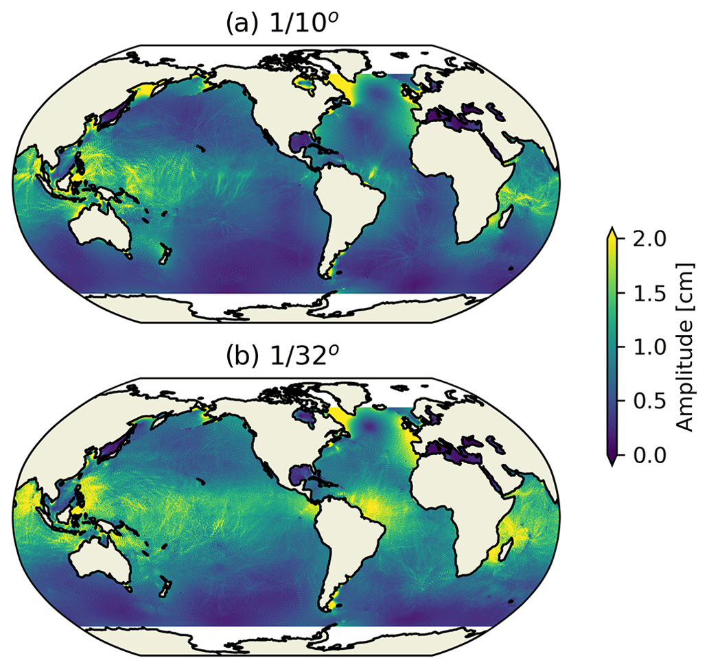
Figure 9Incoherent tide amplitude of semi-diurnal tidal band of the (a) and ∘ (b) models.
3.2 Effects of surface-wave–tide–circulation coupling
Prior to examining the effects of surface-wave-induced mixing in the newly established FIO-COM32 model, the accuracy of the ocean wave model is evaluated. Figure 10 shows the comparisons of satellite data from Jason-3 and model-simulated significant wave height (SWH). From the comparison, the model results are interpolated onto the satellite ground tracks. Both the distributions and seasonal cycle can be reproduced well by the global ∘ resolution surface wave model. The RMSE of the simulated SWH is calculated against the Jason-3 along-track geophysical data records. The Jason-3 data are produced and distributed by AVISO (Archiving, Validation, and Interpolation of Satellite Oceanographic data, http://www.aviso.altimetry.fr/en/home.html, last access: 17 March 2023). We use the low-pass-filtered Jason-3 data for the comparison, and the global mean RMSE of the simulated SWH in 2018 and 2019 is 0.57 m.
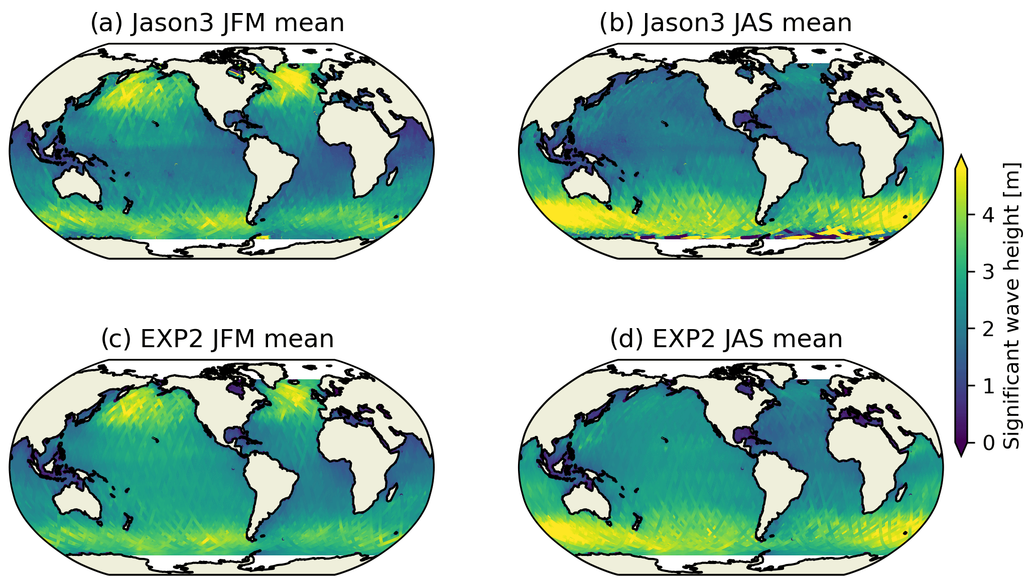
Figure 10Along-track seasonal mean significant wave height of Jason-3 (a, b) and EXP2 (c, d) data. Note that the surface wave model of EXP2 is offline and has a horizontal resolution of ∘.
The ocean upper mixed layer is a crucial layer located between the ocean interior and atmosphere. The MLD determines the heat and momentum content of the upper-ocean boundary layer and is a key factor that reflects the ability of an ocean model. Figure 11 shows the derived summer MLD based on Argo observations (Fig. 11a) and EXP1 (Fig. 11b) and EXP2 (Fig. 11c) simulations. The summer is the mean of July, August and September (JAS) for the Northern Hemisphere and the mean of January, February and March (JFM) for the Southern Hemisphere. The MLD is defined as the depth at which potential density increases by 0.125 kg m−3 from the corresponding surface values. The model results are interpolated onto the Argo profiles in both space and time.

Figure 11Summer (JAS and JFM for the Northern Hemisphere and Southern Hemisphere, respectively) MLD based on Argo observations (a) and EXP1 (b) and EXP2 (c) simulations. The difference in MLD between EXP1 and Argo and between EXP2 and EXP1 and the zonal mean MLD are shown in (d), (e), and (f), respectively.
Both EXP1 and EXP2 are able to reproduce the general patterns of summer MLD distributions. However, the MLD of EXP1 without BV is shallower than that of Argo observations in most of the extratropical regions (Fig. 11d). These shallow biases are significantly alleviated in EXP2 (Fig. 11e), which is due to the inclusion of BV (as previous work has shown). The comparison of the zonal mean MLD shows great improvement in EXP2 over EXP1. EXP2 fits quite well with the observations, except in the Antarctic Circumpolar Current regions. The mean error in MLD at mid-latitudes (10–40∘ N/S) decreases from −4.8 (EXP1) to −0.6 m (EXP2). Although the resolution is increased to ∘, the BV is still an important contributor that improves the summer MLD simulations. The impact of BV in the ∘ model is quite similar to that of the ∘ model (not shown), which means increasing horizontal resolution alone does not solve the long-standing MLD shallow biases in summer. As BV deepens the simulated summer MLD, we further investigate whether it has a detectable effect on the length scale of the surface mixed-layer instability (MLI) (Lsml). We follow Dong et al. (2020b) to calculate the Lsml, which is defined as
where the NML is the depth-averaged buoyancy frequency of the mixed layer and HML is the MLD determined by the relative variance methods (Huang et al., 2018). As shown in Fig. 12, compared with the Argo data, the Lsml of EXP1 with the KPP vertical mixing scheme has a negative bias in most regions similar to that of Dong et al. (2020b), and the Lsml of EXP2 with BV is improved and conforms better with that of the Argo data (Fig. 12d).

Figure 12Length scale of summer (JAS and JFM for the Northern Hemisphere and Southern Hemisphere, respectively) surface mixed-layer instability (Lsml) of Argo observations (a). The differences in Lsml between EXP1 and Argo and between EXP2 and EXP1 and the zonal mean Lsml are shown in (b), (c) and (d), respectively. The mean error in Lsml decreases from −0.96 km in EXP1 to 0.05 km in EXP2.
As the model resolution is increased and global tide is explicitly included in EXP2, the model is able to simulate global internal tide (IT), which is activated when tidal currents flow over rough topography. Since a large portion of barotropic-to-baroclinic energy transfer can be explicitly resolved in EXP2, we disable the parameterised topography drag that has been used in the barotropic model. Figure 13 compares the global internal tide fields of satellite MIOST (Multivariate Inversion of Ocean Surface Topography) (Ubelmann et al., 2022) and model simulations. We apply the radial filter with a radius of 4∘ as a high-pass filter to remove the barotropic tide signals in the open ocean in the model SSH output. Then, harmonic analysis of 1-year high-pass SSH time series is performed to obtain the simulated M2 internal tide amplitude. As shown in Fig. 13, for both the M2 and K1 constituents, the MIOST and EXP2 agree well with each other in terms of the positions of the IT “hot spot” generation sites and the long-range propagation patterns. For example, the well-known generation site of M2 IT near Hawaii and world's strongest K1 IT near Luzon Strait are reproduced well in the model. The model simulations tend to be more energetic than the MIOST data, and whether this bias is due to the mesoscale contamination of the satellite data in the MIOST or insufficient IT-related energy dissipation in present model remains to be explored in the future. The globally averaged bias of amplitude of M2 internal tide at the sea surface is 0.7 cm. Some published global baroclinic tide models such as HYCOM (Arbic et al., 2012; Shriver et al., 2012) show a more conformed internal tide amplitude when compared to the satellite observations than this paper. This may due to the fact that the topographic drag used in their model damps both the amplitude of barotropic and internal tide, while we do not use this kind of dissipation scheme in EXP2.

Figure 13M2 internal tide amplitude at the surface from MIOST (a) and EXP2 (b); (c) and (d) are the same as (a) and (b) but for K1.
Previous studies (SK12, CX17) reported that the high-resolution model-simulated SSH wavenumber spectral slope in the 70–250 km mesoscale domain is quite different from that of satellite observations. In the previous models, the slopes range between −5 and −4 in both low- and high-latitude regions. While the satellite observations show strong latitudinal variability, with a much flatter slope of about −1 in tropical ocean that increases to about −5 and −4 in high-latitude and high-EKE regions. CX21 showed that internal tide-induced SSH signals are a critical factor influencing the wavenumber spectral slopes. With tide included, the wavenumber spectral slopes in the 70–250 km mesoscale range of their ∘ Atlantic regional ocean model show much better agreement with those of satellite observations than the model results without tide. Figure 13 shows that the internal tide-induced sea surface undulations with spatial scale of tens to hundreds kilometres can reach several centimetres, and thus there is a need to explore the different responses of wavenumber spectral slopes in EXP1 and EXP2.
The SSH wavenumber spectral slope in the 70–250 km range is calculated as follows. First, the model SSH data are interpolated onto Jason-3 ground tracks. Second, the spectral slopes are calculated on a 1∘ × 1∘ grid for the global ocean. For each grid point, tracks falling into a 10∘ × 10∘ super-domain centred at the grid point are taken for spectral calculation. In addition, it also requires sub-tracks that are longer than 500 km and that have 90 % or more good-quality data. Prior to spectral analysis, the trend of each sub-track is removed, and a Hanning window is applied. The spectra is obtained by averaging all the SSH spectra obtained via a fast Fourier transform (FFT). Finally, the spectral slope is calculated in the 70–250 km mesoscale range, which is in line with Xu and Fu (2012).
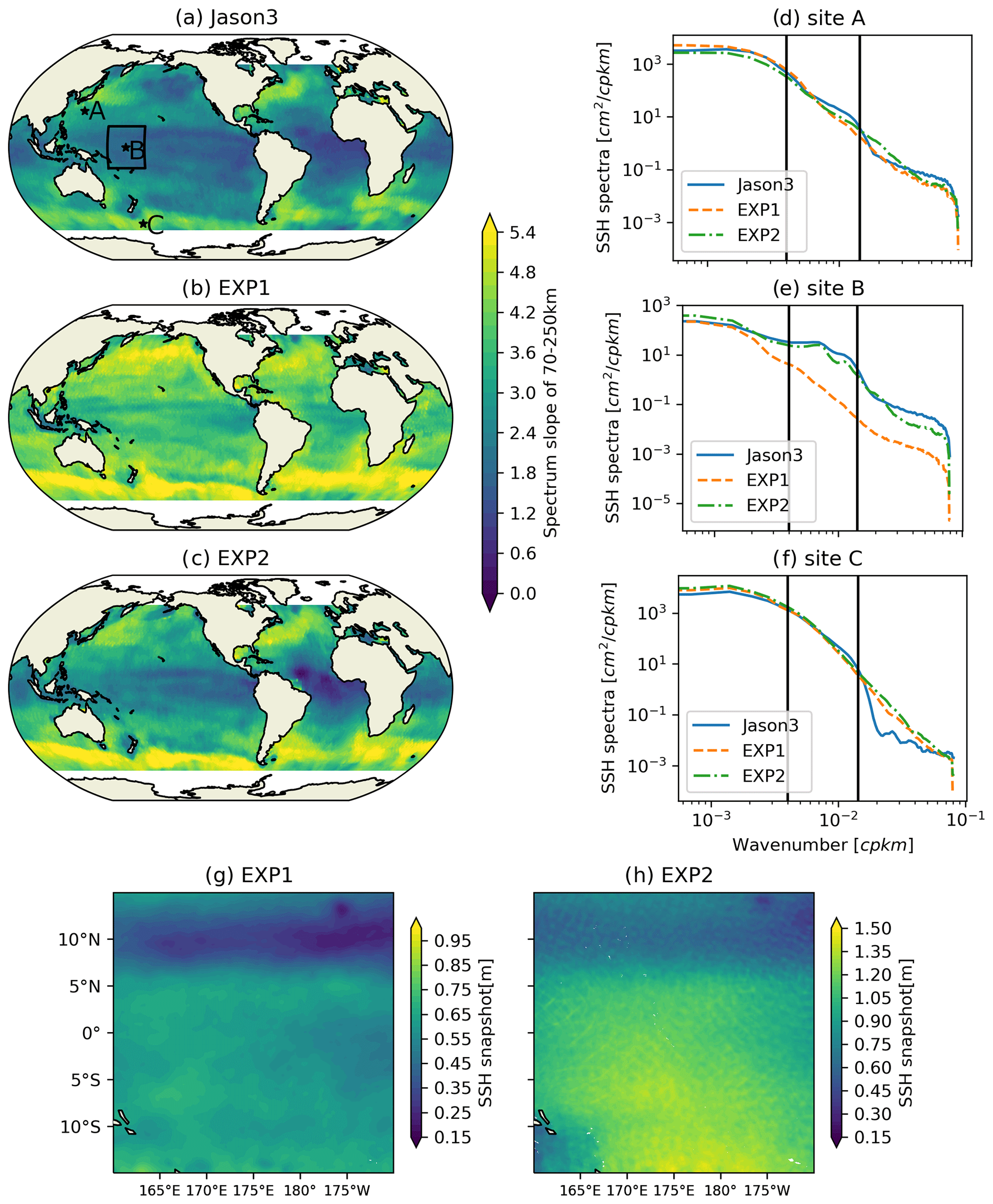
Figure 14SSH wavenumber spectrum slope of 70–250 km in the Jason-3 along-track data (a), EXP1 (b) and EXP2 (c). SSH wavenumber spectrum at three sites in regions of the Kuroshio (d), tropical Pacific Ocean (e) and Southern Ocean (f); the black lines denote the wavenumber at 70 and 250 km. Snapshots of SSH from EXP1 (g) and EXP2 (h) on 1 December 2018 in the region shown with the rectangle in (a). Note that the sign of the spectrum slope is reversed to make it positive in (a)–(c).
Figure 14a, b and c show SSH wavenumber spectral slopes of 70–250 km range of Jason-3 along-track filtered data for EXP1 and EXP2. Figure 14a resembles the results of Xu and Fu (2012), which shows the strong latitudinal variability in wavenumber spectral slopes in the satellite observations. Figure 14b shows the wavenumber spectral slopes of EXP1 have much weaker latitudinal variability, which resemble that of SK12 and CX17. The wavenumber spectral slopes of EXP2 show substantially improved agreement with those of satellite observations shown in Fig. 14a. The flattened wavenumber spectral slopes of EXP2 in low-EKE regions result from internal tide-induced SSH undulations that can be clearly observed in SSH snapshots (see Figs. 14g and h and the Hovmöller diagram in Fig. A5). These internal tide signals have spatial scales of tens to hundreds of kilometres and become nontrivial where the background eddy and circulation field is relatively weak. Figure 14d, e and f show wavenumber spectra at three representative sites. Three locations are chosen for representing typical conditions: (i) high EKE and active internal tides, (ii) typical equatorial regions, and (iii) high EKE but inactive internal tides. In the high-latitude and high-EKE regions, the spectra are less affected by the internal tide signals. However, in the low-latitude and low-EKE regions, the presence of internal tide substantially alters the spectra and yields much more realistic simulations. The textures of SSH in EXP1 and EXP2 shown in Fig. 14g and h manifest many differences that mainly result from the internal tide signals, and EXP2 would be much closer to reality. Therefore, for high-resolution global ocean models, tide–circulation coupling is important for more detailed and realistic SSH simulations. Although the slopes of EXP2 (Fig. 14c) are more in agreement with the observations than those of EXP1 (Fig. 14b), there are still some discrepancies, especially in the low-latitude regions of the Atlantic. In this region, the slope of EXP2 is apparently more flat than the observations, which may indicate that the internal tide is stronger here than normal. A more realistic internal tidal field may further improve the agreement between the model and observations.
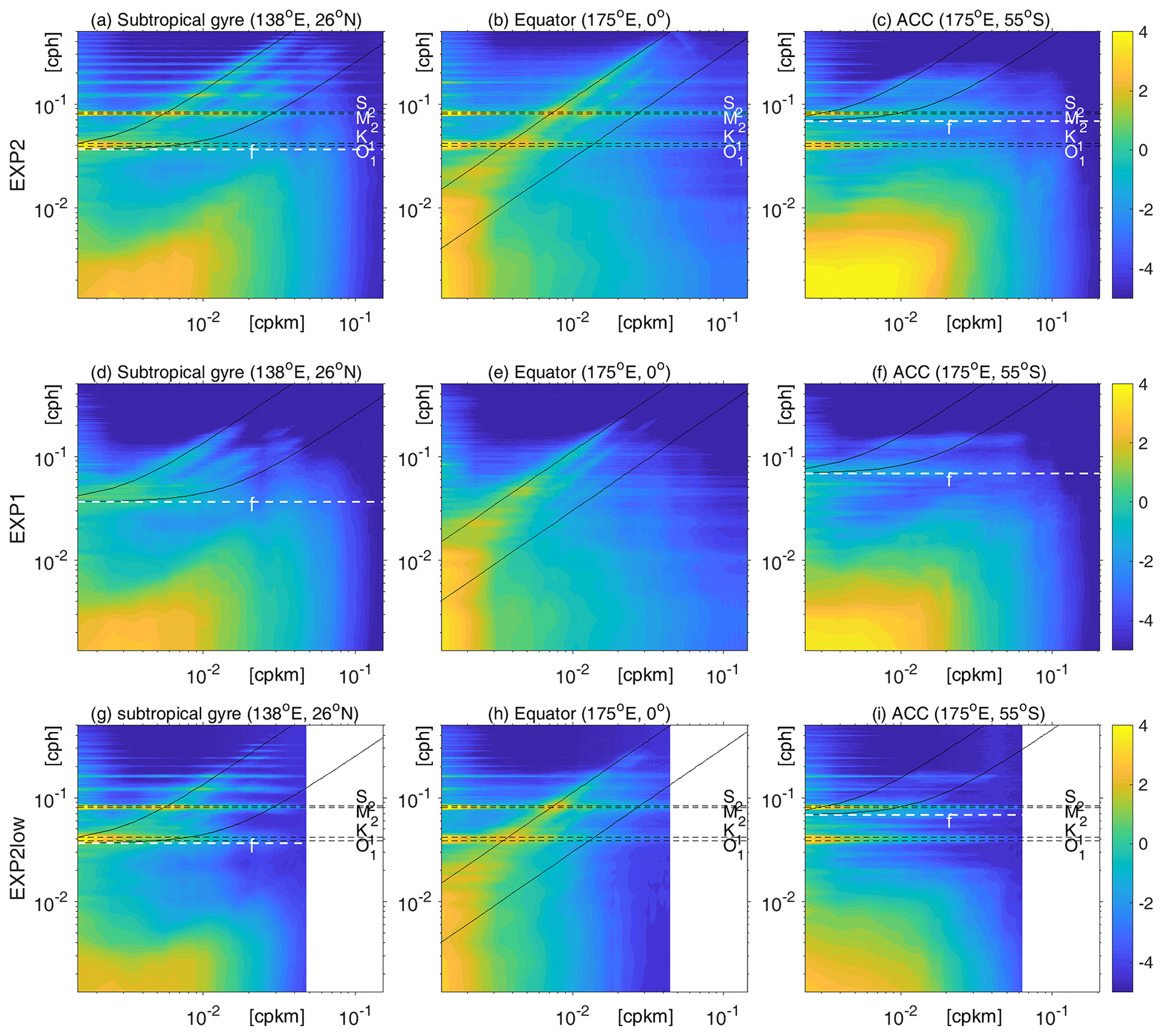
Figure 15SSH variance spectrum amplitude [m2 (cpkm × cph)−1] in horizontal wavenumber–frequency space estimated from 10∘ × 10∘ boxes centred at 26∘ N, 138∘ E (a, d, g), 0∘ N/S, 175∘ E (b, e, h), and 55∘ S, 175∘ E (c, f, i). The upper and middle panels are based on hourly outputs of EXP2 and EXP1, respectively, and the lower panels are based on the ∘ EXP2Low outputs. Dashed white lines denote the inertial frequencies, and dashed black lines denote the tidal constituents of S2, M2, K1, and O1. Solid black curves denote the dispersion relations for inertia-gravity waves of the 1st (upper) and 10th (lower) vertical modes. Note that the colour scale is exponential.
To further explore how the tide–circulation coupling and the increased resolution affect the simulations of different processes (including the rotational processes of sub-mesoscale turbulence and divergent processes of inertial gravity waves, IGWs), the wavenumber–frequency spectra of SSH variance are calculated from the hourly outputs of EXP1, EXP2 and EXP2Low simulations. Focusing on the high-frequency sub-mesoscale processes, the wavenumber–frequency spectra are calculated every 30 d and average the results to obtain a spectral estimate. Before calculating the discrete Fourier transform (DFT), we remove linear trends and multiply the data using a three-dimensional Hanning window. Meanwhile, the dispersion curves of IGWs are estimated from the World Ocean Atlas 2013 climatological temperature–salinity profiles (Qiu et al., 2018).
With respect to sub-mesoscale IGWs, these are shown by clear discrete beams above the 10th vertical normal mode curve in EXP2 (Fig. 15a–c), especially in the subtropical gyre of the western Pacific, which is invisible in EXP1 (Fig. 15d–f). By comparing the SSH wavenumber–frequency spectrum of EXP1 and EXP2, it shows that SSH wavenumber–frequency spectra are more energetic after including tidal forcing in the near-inertial, diurnal and semi-diurnal tidal frequency bands and along the dispersion curves of discrete vertical modes of inertial-gravity waves. This can further explain how the substantially enhanced unbalanced motions (according to Chereskin et al., 2019, “unbalanced motions” refers to the ageostrophic motions, but here the term mainly refers to internal tides and inertia-gravity waves) are responsible for the better match of EXP2 to Jason-3 than EXP1 in Fig. 14. As shown in Fig. 15a–b, in the regions with active IGWs, the energy distribution extends continuously from the sub-mesoscale regime to the IGW regime, which may indicate a strong non-linear interaction between them. However, in the low-resolution experiments shown in Fig. 15g–h there is either a gap between the sub-mesoscale and IGW regimes or insufficient sub-mesoscale activities, which may limit the non-linear interaction between them. It is obvious that SSH variance density is more energetic in the sub-mesoscale regime as resolution increases (<50 km and below the dispersion relation curve associated with the 10th vertical normal mode).
In this paper, for the first time a global ∘ surface-wave–tide–circulation coupled model of FIO-COM32 is developed and validated. Increasing the model horizontal resolution from to ∘ leads to significant improvements in the simulation of surface EKE, the main paths of the Kuroshio and Gulf Stream, and global tides. We proposed ICRE as a quantitative criteria to evaluate the simulated main paths of the Kuroshio and Gulf Stream. As the model horizontal resolution increases from to ∘, the ICRE of the simulated Kuroshio (Gulf Stream) path is decreased from 3.01 × 10¹¹ (4.85 × 10¹¹) to 1.73 × 10¹¹ (3.27 × 10¹¹) m2. The RMSE of the EKE between the model simulations and satellite observations decreased from 63.5 cm2 s−2 in the ∘ model to 31.7 cm2 s−2 in the ∘ model. The global barotropic M2 RMSE decreased from 9.65 cm in the ∘ model to 8.06 cm in the ∘ model. Although the resolution has been increased to ∘, the non-breaking wave-induced mixing (BV) is still a key factor in improving the summer MLD simulation against the Argo observations, with the mean error in the mid-latitude summer MLD reduced from −4.8 m in the numerical experiment without BV to −0.6 m with BV. Internal tides can be explicitly simulated in this new model, and global comparisons of along-track SSH wavenumber spectral slopes in 70–250 km domain show that the internal tide-induced SSH undulations are critical to substantially improved agreement between the global ∘ model and satellite data, indicating that tide is a generator of sub-mesoscale process.
In future work, the effects of sea surface currents (SSCs) on surface wave simulation need to be taken into consideration for a fully coupled wave–circulation model, as this phenomenon has been shown to have impact on surface wave simulation (Ardhuin et al., 2017). As has been stated in this paper, the online coupled surface-wave–ocean circulation version of the FIO-COM32 is turned off pro tempore and is ready to be implemented when the demands for greater computational resources are met in the near future, and at that time the effects of ocean currents on the surface waves will be explored in depth. Figure 16 shows an example of the effect of SSCs on the simulated significant wave height. The hourly SSC output from FIO-COM32 in the western Pacific is fed into the MASNUM wave model to test SSC effects on surface waves. It is clear that SSCs have a notable influence on the simulated significant wave height, especially around the Kuroshio. In MASNUM wave model, SSCs influence the surface wave simulations through advection, refraction and the energy source function due to interaction between surface waves and SSC shear (Yang et al., 2005).
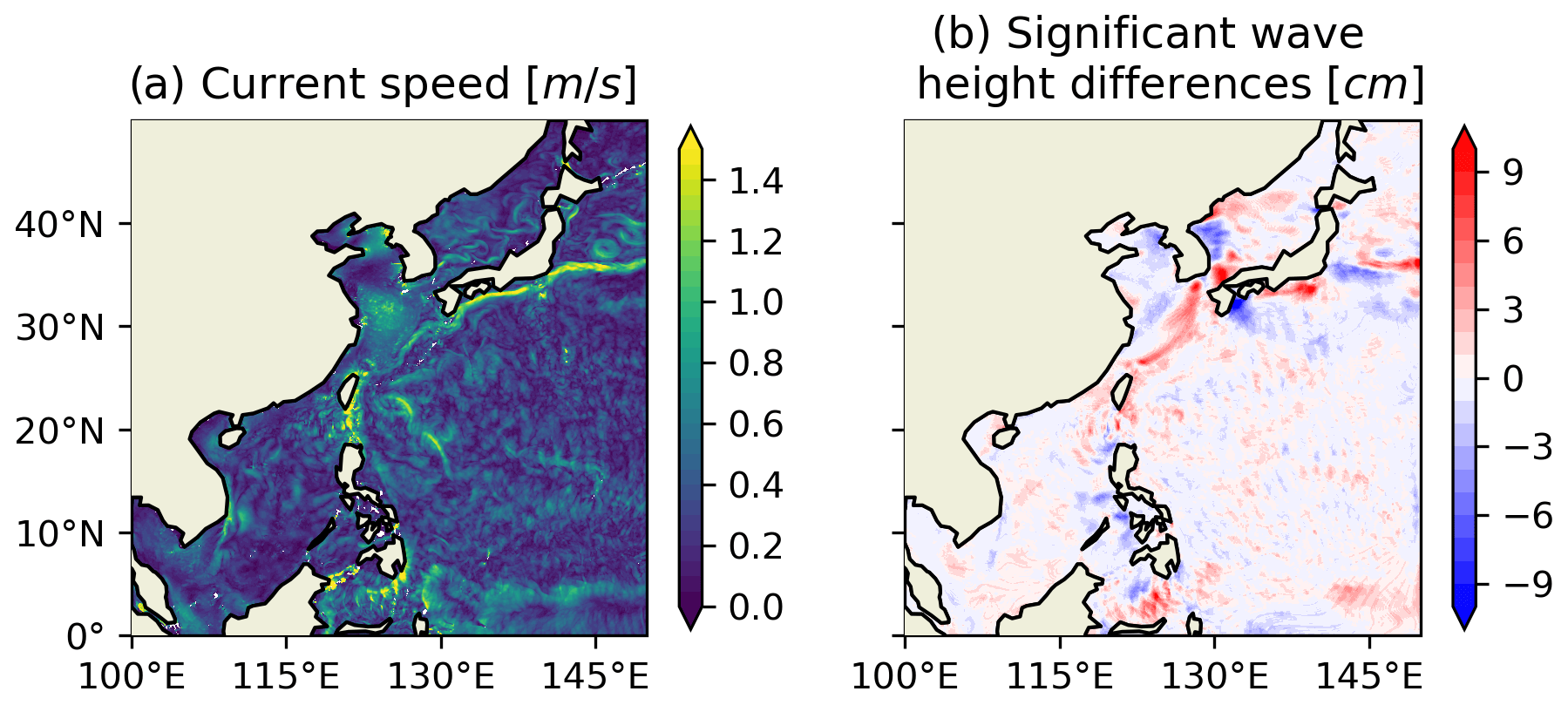
Figure 16(a) Sea surface current (SSC) snapshot of 8 October 2018. (b) The differences in significant wave height between MASNUM wave models with and without SSC effects.
Since the internal tide can be resolved in the FIO-COM32 model, finding a more robust representation of energy dissipation of internal tide propagation is still an open task that needs to be addressed in the future. A proper dissipation scheme of the internal tide and its adaption to the traditional viscosity schemes for OGCM is still a daunting challenge. We have conducted numerical experiments (not shown) with an inordinately large background vertical viscosity of 1.0 m2 s−1, and in these experiments the amplitude of the simulated internal tide is brought down to the comparable level of the MIOST observations. These preliminary explorations indicate that a proper scheme of vertical mixing considering the internal gravity wave dissipation in the tide–circulation coupled ocean model needs to be developed. At the same time, proper representation of the unresolved barotropic-to-baroclinic tidal conversion also needs to be considered. More realistic treatments of SAL will improve the accuracy of global barotropic tide models (Arbic et al., 2004).
A better prediction of ocean is the inexhaustible goal of the ocean model community. As the ocean, especially the upper ocean, plays a dominant role in the climate system, ocean model improvement can shed light on new generations of climate model development. Surface waves, tides and ocean circulations are often separately simulated by different numerical models. In this paper, we show that surface wave–tide–circulation coupling can dramatically improve simulations. Therefore, it is time for us to regard the ocean as a fully coupled dynamic system through the key conjunction of turbulence and develop fully coupled surface-wave–internal-wave–tide–circulation models for the next generation of ocean model development.
Since the time span of the numerical experiments is not long (3.5 years), the model drift is generally quite small. The model drift in temperature shows a strong seasonal cycle in the upper ocean and a warming trend in the sub-surface layer, and the maximum drift in temperature at the end is about 0.2∘ (Fig. A2a). The upper 150 m becomes slightly salty, and the sub-surface layer shows freshening drift, while the salinity drift value is generally small, i.e. less than 0.02 PSU (Fig. A2b). The zonal mean temperature and salinity and their corresponding drifts are displayed in Figs. A2c–f, and the zonal mean drifts are moderate.
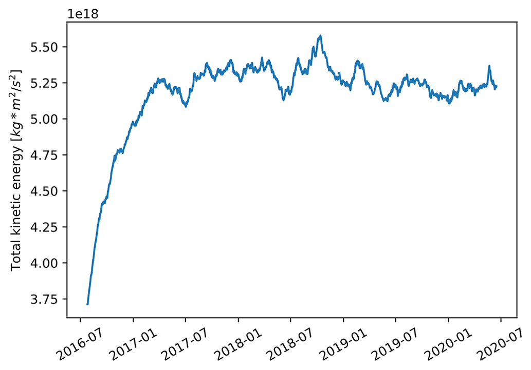
Figure A1Time series of simulated total kinetic energy of EXP1. Figure A1 shows the total kinetic energy of EXP1 since the beginning of the numerical experiment. The ∘ model starts from a ∘ model state and enters a new steady state after a swift adjustment period of about 1 year. After the short spin-up period, the total kinetic energy reaches quasi-steady state with small fluctuations.
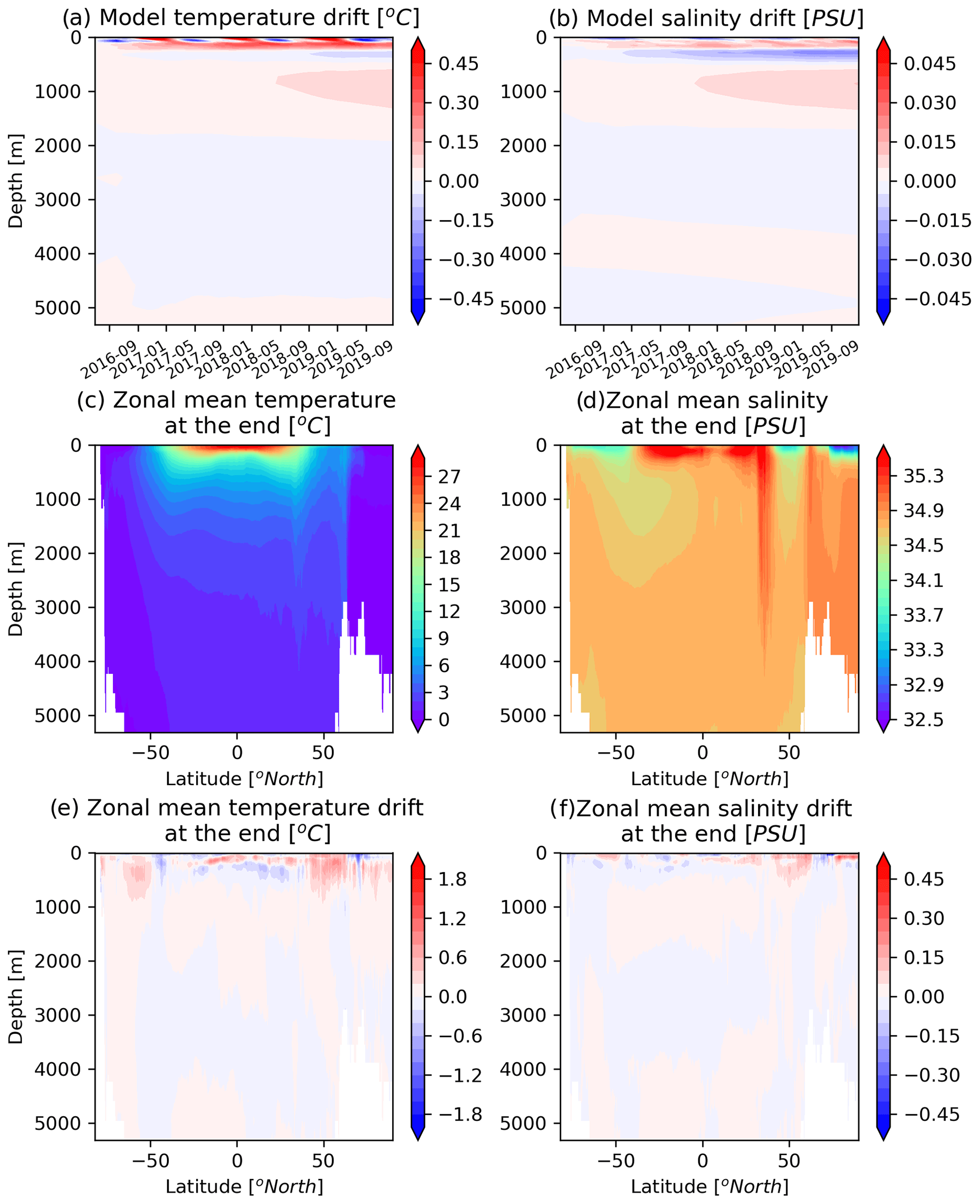
Figure A2Model drift of temperature (a) and salinity (b), zonally averaged temperature (c), salinity (d), and the corresponding drift (e, f) at the end of EXP1. As the last day of model integration is 31 December 2019, the drifts in (e) and (f) are calculated using the simulation difference between December 2016 and December 2019.
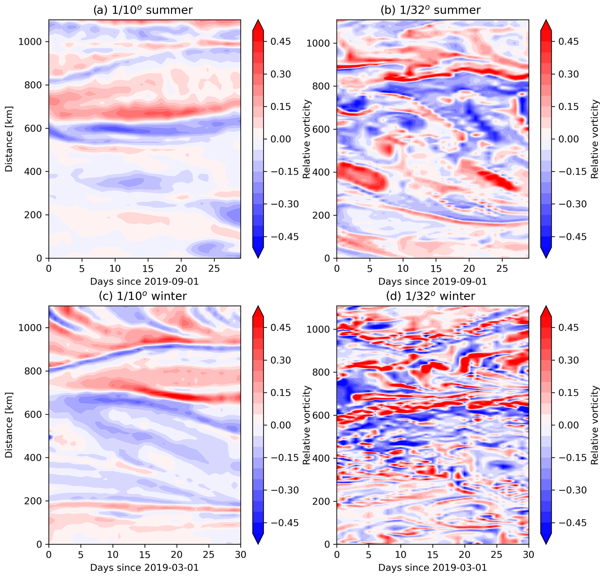
Figure A3Hovmöller diagram of surface relative vorticity along a section in the Kuroshio Extension region, marked as black line shown in Fig. 6a.
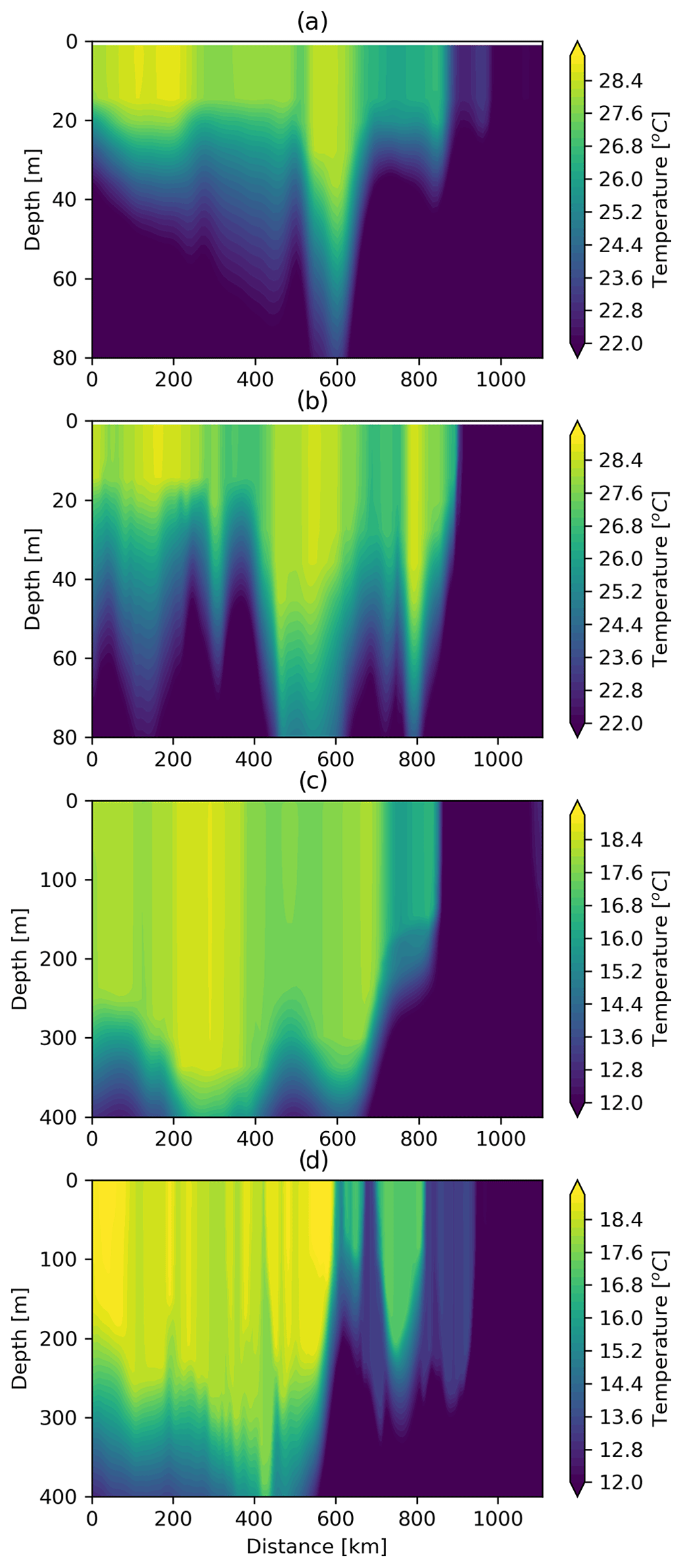
Figure A4Temperature along the section in the Kuroshio Extension region of (a, c) and ∘ (b, d) models during summer (a, b) and winter (c, d), respectively. Figures A3 and A4 show the evolution of relative vorticity and temperature along a typical section in the Kuroshio Extension region, which is shown in Fig. 6a. The typical horizontal scale of resolved fronts in the ∘ model is about 60 km, and the horizontal scale in the ∘ model is about 3 times smaller (∼ 20 km). The vertical scales of the resolved fronts of both the model and ∘ model are quite similar, and the summer (winter) has a vertical scale of about 30 m (300 m).
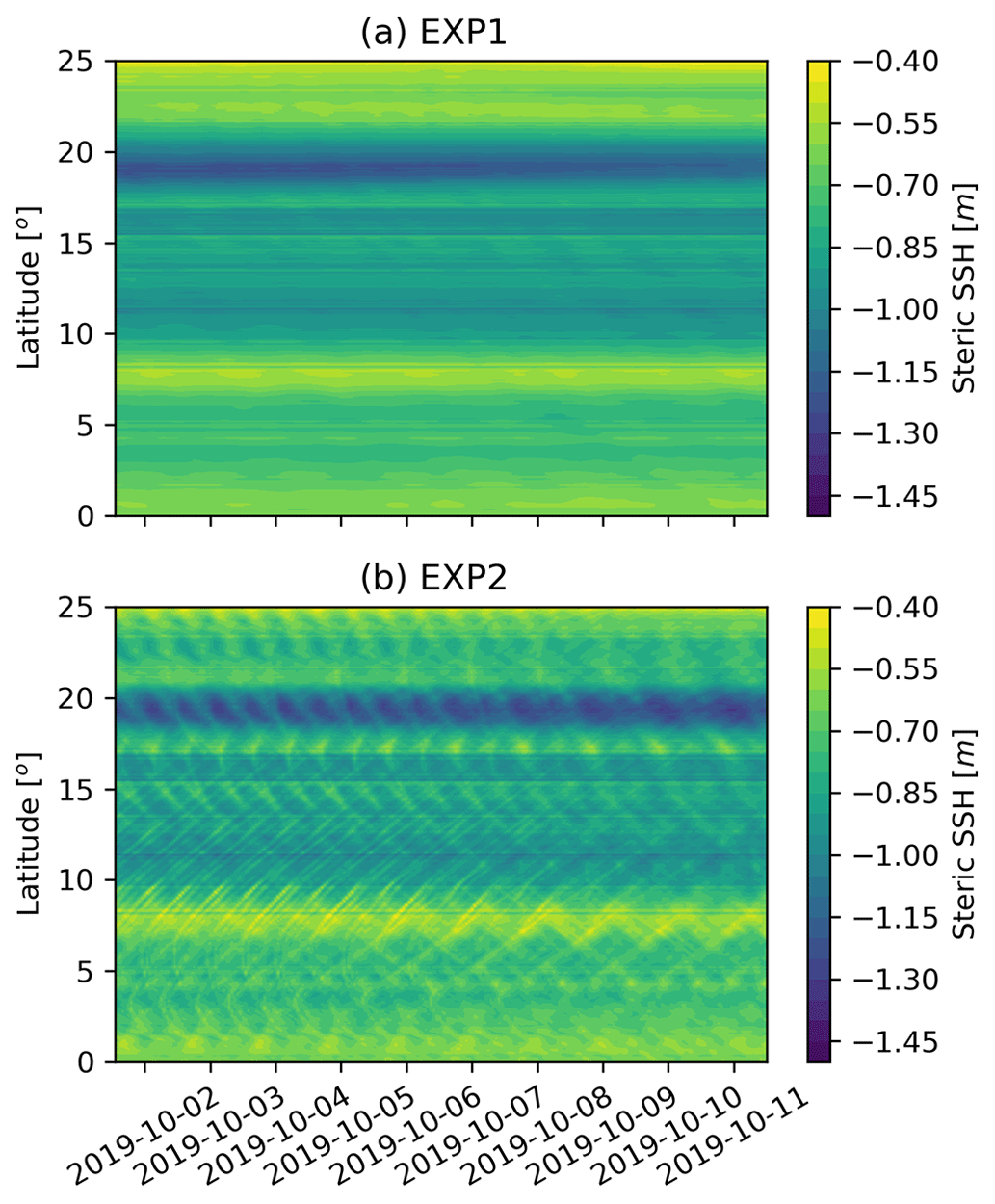
Figure A5Hovmöller diagram of steric SSH along the section of 135∘ E. EXP2 with tide shows obvious signals of the propagation of internal tide. This figure, together with Fig. 14g–h, explains how the internal tide signature affects the simulated SSH.
The exact version of the model, input data used to produce the results in this paper and data to produce the plots are archived on Zenodo (https://doi.org/10.5281/zenodo.6221095, Xiao et al., 2022), and the minimal scripts required to compile and run the model can be accessed on GitHub (https://github.com/mom-ocean/MOM5, GFDL, 2023). The atmosphere forcing data can be downloaded from https://www.nco.ncep.noaa.gov/pmb/products/gfs/ (NCEP, 2023).
BX was responsible for model development and drafted the manuscript. FQ designed the road map of this research and supervised the writing of the paper. All authors contributed to discussions, data analysis and writing of the paper.
The contact author has declared that none of the authors has any competing interests.
Publisher’s note: Copernicus Publications remains neutral with regard to jurisdictional claims in published maps and institutional affiliations.
This research is jointly supported by the National Natural Science Foundation of China under grant no. 41821004 and the Marine S&T Fund of Shandong Province for the Pilot National Laboratory for Marine Science and Technology (Qingdao) (grant no. 2018SDKJ0106-1). This work is a contribution to the UN Decade of Ocean Science for Sustainable Development (2021–2030) through both the Decade Collaborative Centre on Ocean-Climate Nexus and Coordination Amongst Decade Implementing Partners in P.R. China (DCC-OCC) and the approved programme of the Ocean to climate Seamless Forecasting system (OSF).
This research is jointly supported by the National Natural Science Foundation of China under grant no. 41821004 and the Marine S&T Fund of Shandong Province for the Pilot National Laboratory for Marine Science and Technology (Qingdao) (grant no. 2018SDKJ0106-1).
This paper was edited by Riccardo Farneti and reviewed by two anonymous referees.
Adcroft, A., Hill, C., and Marshall, J.: Representation of topography by shaved cells in a height coordinate ocean model, Mon. Weather Rev., 125, 2293–2315, 1997.
Adcroft, A. J. and Campin, J. M.: Rescaled height coordinates for accurate representation of free-surface flows in ocean circulation models, Ocean Model., 7, 269–284, 2004.
Ajayi, A., Le Sommer, J., Chassignet, E., Molines, J.-M., Xu, X., Albert, A., and Cosme, E.: Spatial and temporal variability of the north Atlantic eddy field from two kilometric-resolution ocean models, J. Geophys. Res., 125, e2019JC015827, https://doi.org/10.1029/2019JC015827, 2020.
Amores, A., Jordà, G., Arsouze, T., and Le Sommer, J.: Up to what extent can we characterize ocean eddies using present-day gridded altimetric products?, J. Geophys. Res., 123, 7220-7236, https://doi.org/10.1029/2018JC014140, 2018.
Ansong, J. K., Arbic, B. K., Simmons, H. L., Alford, M. H., Buijsman, M. C., Timko, P. G., Richman, J. G., Shriver, J. F., and Wallcraft, A. J.: Geographical Distribution of diurnal and semidiurnal parametric subharmonic instability in a Global Ocean Circulation Model, J. Phys. Oceanogr., 48, 1409–1431, https://doi.org/10.1175/jpo-d-17-0164.1, 2018.
Arbic, B. K., Garner, S. T., Hallberg, R. W., and Simmons, H. L.: The accuracy of surface elevations in forward global barotropic and baroclinic tide models, Deep-Sea Res. Pt. II, 51, 3069–3101, 2004.
Arbic, B. K., Wallcraft, A. J., and Metzger, E. J.: Concurrent simulation of the eddying general circulation and tides in a global ocean model, Ocean Model., 32, 175–187, 2010.
Arbic, B. K., Richman, J. G., Shriver, J. F., Timko, P. G., Metzger, E. J., and Wallcraft, A. J.: Global modeling of internal tides within an eddying Ocean General Circulation Model, Oceanography, 25, 20–29, https://doi.org/10.5670/oceanog.2012.38, 2012.
Arbic, B., Alford, M., Ansong, J., Buijsman, M., Ciotti, R., Farrar, J., Hallberg, R., Henze, C., Hill, C., Luecke, C., Menemenlis, D., Metzger, E., Müeller, M., Nelson, A., Nelson, B., Ngodock, H., Ponte, R., Richman, J., Savage, A., and Zhao, Z.: A primer on global internal tide and internal gravity wave continuum modeling in HYCOM and MITgcm, in: New Frontiers in Operational Oceanography, GODAE OceanView, 307–392, https://doi.org/10.17125/gov2018.ch13, 2018.
Ardhuin, F., Gille, S. T., Menemenlis, D., Rocha, C. B., Rascle, N., Chapron, B., Gula, J., and Molemaker, J.: Small-scale open ocean currents have large effects on wind wave heights, J. Geophys. Res.-Oceans, 122, 4500–4517, https://doi.org/10.1002/2016JC012413, 2017.
Biri, S., Serra, N., Scharffenberg, M. G., and Stammer, D.: Atlantic sea surface height and velocity spectra inferred from satellite altimetry and a hierarchy of numerical simulations, J. Geophys. Res., 121, 4157–4177, https://doi.org/10.1002/2015JC011503, 2016.
Bryan, K. and Cox, M. D.: A numerical investigation of the oceanic general circulation, Tellus A, 19, 54–80, https://doi.org/10.1111/j.2153-3490.1967.tb01459.x, 1967.
Buijsman, M. C., Arbic, B. K., Green, J. A. M., Helber, R. W., Richman, J. G., Shriver, J. F., Timko, P. G., and Wallcraft, A.: Optimizing internal wave drag in a forward barotropic model with semidiurnal tides, Ocean Model., 85, 42–55, 2015.
Capet, X., Roullet, G., Klein, P., and Maze, G.: Intensification of Upper-Ocean Submesoscale Turbulence through Charney Baroclinic Instability, J. Phys. Oceanogr., 46, 3365–3384, https://doi.org/10.1175/jpo-d-16-0050.1, 2016.
Chassignet, E. P. and Xu, X.: Impact of horizontal resolution (1/12∘ to ∘) on Gulf Stream separation, penetration, and variability, J. Phys. Oceanogr., 47, 1999–2021, https://doi.org/10.1175/JPO-D-17-0031.1, 2017.
Chassignet, E. P. and Xu, X.: On the importance of high-resolution in large-scale ocean models, Adv. Atmos. Sci., 38, 1621–1634, https://doi.org/10.1007/s00376-021-0385-7, 2021.
Chen, S., Qiao, F., Huang, C., and Song, Z.: Effects of the non-breaking surface wave-induced vertical mixing on winter mixed layer depth in subtropical regions, J. Geophys. Res., 123, 2934–2944, https://doi.org/10.1002/2017JC013038, 2018.
Chereskin, T. K., Rocha, C. B., Gille, S. T., Menemenlis, D., and Passaro, M.: Characterizing thetransition from balanced to unbalanced motions in the southern California Current, J. Geophys. Res.-Oceans, 124, 2088–2109, https://doi.org/10.1029/2018JC014583, 2019.
Dong, J., Fox-Kemper, B., Zhang, H., and Dong, C.: The seasonality of submesoscale energy production, content, and cascade, Geophys. Res. Lett., 47, e2020GL087388, https://doi.org/10.1029/2020GL087388, 2020a.
Dong, J., Fox-Kemper, B., Zhang, H., and Dong, C.: The scale of submesoscale baroclinic instability globally, J. Phys. Oceanogr., 50, 2649–2667, https://doi.org/10.1175/JPO-D-20-0043.1, 2020b.
Egbert, G. D., Ray, R. D., and Bills, B. G.: Numerical modeling of the global semidiurnal tide in the present day and in the last glacial maximum, J. Geophys. Res., 109, C03003, https://doi.org/10.1029/2003JC001973, 2004.
Fan, Y. and Griffies, S. M.: Impacts of parameterized Langmuir turbulence and nonbreaking wave mixing in global climate simulations, J. Climate, 27, 4752–4775, 2014.
Fretwell, P., Pritchard, H. D., Vaughan, D. G., Bamber, J. L., Barrand, N. E., Bell, R., Bianchi, C., Bingham, R. G., Blankenship, D. D., Casassa, G., Catania, G., Callens, D., Conway, H., Cook, A. J., Corr, H. F. J., Damaske, D., Damm, V., Ferraccioli, F., Forsberg, R., Fujita, S., Gim, Y., Gogineni, P., Griggs, J. A., Hindmarsh, R. C. A., Holmlund, P., Holt, J. W., Jacobel, R. W., Jenkins, A., Jokat, W., Jordan, T., King, E. C., Kohler, J., Krabill, W., Riger-Kusk, M., Langley, K. A., Leitchenkov, G., Leuschen, C., Luyendyk, B. P., Matsuoka, K., Mouginot, J., Nitsche, F. O., Nogi, Y., Nost, O. A., Popov, S. V., Rignot, E., Rippin, D. M., Rivera, A., Roberts, J., Ross, N., Siegert, M. J., Smith, A. M., Steinhage, D., Studinger, M., Sun, B., Tinto, B. K., Welch, B. C., Wilson, D., Young, D. A., Xiangbin, C., and Zirizzotti, A.: Bedmap2: improved ice bed, surface and thickness datasets for Antarctica, The Cryosphere, 7, 375–393, https://doi.org/10.5194/tc-7-375-2013, 2013.
Garrett, C. J. R., Loder, J. W., Swallow, J. C., Currie, R. I., Gill, A. E., and Simpson, J. H.: Dynamical aspects of shallow sea fronts, Philos. T. Roy. Soc. A, 302, 563–581, https://doi.org/10.1098/rsta.1981.0183, 1981.
GFDL: The Modular Ocean Model version 5, GitHub [code], https://github.com/mom-ocean/MOM5, last access: 17 March 2023.
Griffies, S. M.: Elements of the Modular Ocean Model (MOM), NOAA Geophysical Fluid Dynamics Laboratory, NJ, USA, 614–627, 2012.
Hallberg, R.: Using a resolution function to regulate parameterizations of oceanic mesoscale eddy effects, Ocean Model., 72, 92–103, https://doi.org/10.1016/J.OCEMOD.2013.08.007, 2013.
Huang, P. Q., Lu Y. Z., and Zhou S. Q.: An objective method for determining ocean mixed layer depth with applications to WOCE Data, J. Atmos. Ocean. Tech., 35.3, 441–458, https://doi.org/10.1175/JTECH-D-17-0104.1, 2018.
Holt, J. and Umlauf, L.: Modelling the tidal mixing fronts and seasonal stratification of the Northwest European Continental shelf, Cont. Shelf Res., 28, 887–903, https://doi.org/10.1016/j.csr.2008.01.012, 2008.
International Hydrographic Organization, Intergovernmental Oceanographic Commission (IHO-IOC): The IHO-IOC GEBCO Cook Book, IHO Publication B-11, Monaco, 416 pp., 2018.
Jayne, S. R. and St Laurent, L. C.: Parameterizing tidal dissipation over rough topography, Geophys. Res. Lett., 28, 811–814, 2001.
Large, W. G. and Yeager, S.: Diurnal to decadal global forcing for ocean and sea-ice models: The data sets and flux climatologies (No. NCAR/TN-460+STR), University Corporation for Atmospheric Research, https://doi.org/10.5065/D6KK98Q6, 2004.
Large, W. G., McWilliams, J. C., and Doney, S. C.: Oceanic vertical mixing: A review and a model with a nonlocal boundary layer parameterization, Rev. Geophys., 32, 363–403, 1994.
Lévy, M., Klein, P., Tréguier, A. M., Iovino, D., Madec, G., Masson, S., and Takahashi, K.: Modifications of gyre circulation by sub-mesoscale physics, Ocean Model., 34, 1–15, https://doi.org/10.1016/j.ocemod.2010.04.001, 2010.
Lin, L., Liu, D., Guo, X., Luo, C., and Cheng, Y.: Tidal effect on water export rate in the eastern Shelf Seas of China, J. Geophys. Res., 125, e2019JC015863, https://doi.org/10.1029/2019JC015863, 2020.
Lü, X., Qiao, F., Xia, C., Zhu, J., and Yuan, Y.: Upwelling off Yangtze River estuary in summer, J. Geophys. Res.-Oceans, 111, C11S08, https://doi.org/10.1029/2005JC003250, 2006.
Lü, X., Qiao, F., Wang, G., Xia, C., and Yuan, Y.: Upwelling off the west coast of Hainan Island in summer: Its detection and mechanisms, Geophys. Res. Lett., 35, L02604, https://doi.org/10.1029/2007GL032440, 2008.
Lü, X., Qiao, F., Xia, C., Wang, G., and Yuan, Y.: Upwelling and surface cold patches in the Yellow Sea in summer: Effects of tidal mixing on the vertical circulation, Cont. Shelf Res., 30, 620–632, 2010.
McWilliams, J. C. and Fox-Kemper, B.: Oceanic wave-balanced surface fronts and filaments, J. Fluid Mech., 730, 464–490, 2013.
Mellor, G. and Blumberg, A.: Wave breaking and ocean surface layer thermal response, J. Phys. Oceanogr., 34, 693–698, 2004.
Murray, R. J.: Explicit generation of orthogonal grids for ocean models, J. Comput. Phys., 126, 251–273, 1996.
NCEP: The Global Forecast System (GFS), NCEP [data set], https://www.nco.ncep.noaa.gov/pmb/products/gfs/, last access: 17 March 2023.
Qiao, F. and Huang, C. J.: Comparison between vertical shear mixing and surface wave-induced mixing in the extratropical ocean, J. Geophys. Res.-Oceans, 117, C00J16, https://doi.org/10.1029/2012JC007930, 2012.
Qiao, F., Yuan, Y., Yang, Y., Zheng, Q., Xia, C., and Ma, J.: Wave-induced mixing in the upper ocean: Distribution and application to a global ocean circulation model, Geophys. Res. Lett., 31, L11303, https://doi.org/10.1029/2004GL019824, 2004.
Qiao, F., Yuan, Y., Deng, J., Dai, D., and Song, Z.: Wave–turbulence interaction-induced vertical mixing and its effects in ocean and climate models. Phil. Trans. R. Soc. A, 374, 20150201, https://doi.org/10.1098/rsta.2015.0201, 2016.
Qiao, F., Zhao, W., Yin, X., Huang, X., Liu, X., Shu, Q., Wang, G., Song, Z., Li, X., Liu, H., Yang, G., and Yuan, Y.: A highly effective global surface wave numerical simulation with ultra-high resolution, International Conference For High Performance Computing, Networking, Storage And Analysis, Sc.345 E 47th St, New York, Ny 10017 Usa.Ieee.2017-03-13, 46–56, ISBN 978-1-4673-8815-3, http://dl.acm.org/citation.cfm?id=3014904.3014911 (last access: 17 March 2023), 2017.
Qiao, F., Wang, G., Yin, L., Zeng, K., Zhang, Y., Zhang, M., Xiao, B., Jiang, S., Chen, H., and Chen, G.: Modelling oil trajectories and potentially contaminated areas from the Sanchi oil spill, Sci. Total. Environ., 685, 856–866, https://doi.org/10.1016/j.scitotenv.2019.06.255, 2019.
Qiu, B., Chen, S., Klein, P., Wang, J., Torres, H., Fu, L.-L., and Menemenlis, D.: Seasonality in Transition Scale from Balanced to Unbalanced Motions in the World Ocean, J. Phys. Oceanogr., 48, 591–605, https://doi.org/10.1175/JPO-D-17-0169.1, 2018.
Richman, J. G., Arbic, B. K., Shriver, J. F., Metzger, E. J., and Wallcraft, A. J.: Inferring dynamics from the wavenumber spectra of an eddying global ocean model with embedded tides, J. Geophys. Res., 117, C12012, https://doi.org/10.1029/2012JC008364, 2012.
Rocha, C. B., Chereskin, T. K., Gille, S. T., and Menemenlis, D.: Mesoscale to submesoscale wavenumber spectra in Drake Passage, J. Phys. Oceanogr., 46, 601–620, https://doi.org/10.1175/JPO-D-15-0087.1, 2016.
Sasaki, H. and Klein, P.: SSH wavenumber spectra in the North Pacific from a high-resolution realistic simulation, J. Phys. Oceanogr., 42, 1233–1241, https://doi.org/10.1175/JPO-D-11-0180.1, 2012.
Sasaki, H., Klein, P., Sasai, Y., and Qiu, B.: Regionality and seasonality of submesoscale and mesoscale turbulence in the North Pacific Ocean, Ocean Dynam., 67, 1195–1216, https://doi.org/10.1007/s10236-017-1083-y, 2017.
Savage, A. C., Arbic, B. K., Alford, M. H., Ansong, J. K., Farrar, J. T., Menemenlis, D., O'Rourke, A. K., Richman, J. G., Shriver, J. F., Voet, G., Wallcraft, A. J., and Zamudio, L.: Spectral decomposition of internal gravity wave sea surface height in global models, J. Geophys. Res.-Oceans, 122, 7803–7821, https://doi.org/10.1002/2017JC013009, 2017a.
Savage, A. C., Arbic, B. K., Richman, J. G., Shriver, J. F., Alford, M. H., Buijsman, M. C., Thomas Farrar, J., Sharma, H., Voet, G., Wallcraft, A. J., and Zamudio, L.: Frequency content of sea surface height variability from internal gravity waves to mesoscale eddies, J. Geophys. Res.-Oceans, 122, 2519–2538, https://doi.org/10.1002/2016JC012331, 2017b.
Schiller, A. and Fiedler, R.: Explicit tidal forcing in an ocean general circulation model, Geophys. Res. Lett., 34, L03611, https://doi.org/10.1029/2006GL028363, 2007.
Shi, J., Yin, X., Shu, Q., Xiao, B., and Qiao, F.: Evaluation on data assimilation of a global high resolution wave-tide-circulation coupled model using the tropical Pacific TAO buoy observations, Acta Oceanol. Sin., 37, 8–20, https://doi.org/10.1007/s13131-018-1196-2, 2018.
Shriver, J., Arbic, B. K., Richman, J., Ray, R., Metzger, E., Wallcraft, A., and Timko, P.: An evaluation of the barotropic and internal tides in a high-resolution global ocean circulation model, J. Geophys. Res., 117, C10024, https://doi.org/10.1029/2012JC008170, 2012.
Shu, Q., Qiao, F., Song, Z., Xia, C., and Yang, Y.: Improvement of MOM4 by including surface wave-induced vertical mixing, Ocean Model., 40, 42–51, 2011.
Simpson, J. H. and Hunter, J. R.: Fronts in the Irish Sea, Nature, 250, 404–406, https://doi.org/10.1038/250404a0, 1974.
Song, Z., Qiao, F., and Song, Y.: Response of the equatorial basin-wide SST to non-breaking surface wave-induced mixing in a climate model: An amendment to tropical bias, J. Geophys. Res., 117, C00J26, https://doi.org/10.1029/2012JC007931, 2012.
Su, Z., Wang, J., Klein, P., Thompson, A. F., and Menemenlis, D.: Ocean submesoscales as a key component of the global heat budget, Nat. Commun., 9, 775, https://doi.org/10.1038/s41467-018-02983-w, 2018.
Sun, Y., Perrie, W., Qiao, F., and Wang, G.: Intercomparisons of highresolution global ocean analyses: Evaluation of a new synthesis in tropical oceans, J. Geophys. Res., 125, e2020JC016118, https://doi.org/10.1029/2020JC016118, 2020.
Suzuki, N., Fox-Kemper, B., Hamlington, P. E., and Roekel, L.: Surface waves affect frontogenesis, J. Geophys. Res.-Oceans, 121, 3597–3624, https://doi.org/10.1002/2015JC011563, 2016.
Teixeira, M. and Belcher, S. E.: On the distortion of turbulence by a progressive surface wave, J. Fluid Mech., 458, 229–267, https://doi.org/10.1017/S0022112002007838, 2002.
Thoppil, P. G., Richman, J. G., and Hogan, P. J.: Energetics of a Global Ocean Circulation Model compared to observations, Geophys. Res. Lett., 38, L15607, https://doi.org/10.1029/2011GL048347, 2011.
Timko, P. G., Arbic, B. K., Hyder, P., Richman, J. G., Zamudio, L., O'Dea, E., Wallcraft, A. J., and Shriver, J. F.: Assessment of shelf sea tides and tidal mixing fronts in a global ocean model, Ocean Model., 136, 66–84, https://doi.org/10.1016/j.ocemod.2019.02.008, 2019.
Ubelmann, C., Carrere, L., Durand, C., Dibarboure, G., Faugère, Y., Ballarotta, M., Briol, F., and Lyard, F.: Simultaneous estimation of ocean mesoscale and coherent internal tide sea surface height signatures from the global altimetry record, Ocean Sci., 18, 469–481, https://doi.org/10.5194/os-18-469-2022, 2022.
Uchida, T., Le Sommer, J., Stern, C., Abernathey, R. P., Holdgraf, C., Albert, A., Brodeau, L., Chassignet, E. P., Xu, X., Gula, J., Roullet, G., Koldunov, N., Danilov, S., Wang, Q., Menemenlis, D., Bricaud, C., Arbic, B. K., Shriver, J. F., Qiao, F., Xiao, B., Biastoch, A., Schubert, R., Fox-Kemper, B., Dewar, W. K., and Wallcraft, A.: Cloud-based framework for inter-comparing submesoscale-permitting realistic ocean models, Geosci. Model Dev., 15, 5829–5856, https://doi.org/10.5194/gmd-15-5829-2022, 2022.
Wang, G., Zhao, C., Xu, J., Qiao, F., and Xia, C.: Verification of an operational ocean circulation-surface wave coupled forecasting system for the China's seas, Acta Oceanol. Sin., 35, 19–28, https://doi.org/10.1007/s13131-016-0810-4, 2016.
Wang, P., Jiang, J., Lin, P., Ding, M., Wei, J., Zhang, F., Zhao, L., Li, Y., Yu, Z., Zheng, W., Yu, Y., Chi, X., and Liu, H.: The GPU version of LASG/IAP Climate System Ocean Model version 3 (LICOM3) under the heterogeneous-compute interface for portability (HIP) framework and its large-scale application , Geosci. Model Dev., 14, 2781–2799, https://doi.org/10.5194/gmd-14-2781-2021, 2021.
Wang, S., Wang, Q., Shu, Q., Scholz, P., Lohmann, G., and Qiao, F.: Improving the upper-ocean temperature in an Ocean Climate Model (FESOM 1.4): Shortwave Penetration Versus Mixing Induced by Nonbreaking Surface Waves, J. Adv. Model. Earth. Sy., 11, 545–557, https://doi.org/10.1029/2018MS001494, 2019.
Wang, Y., Qiao, F., Fang, G., and Wei, Z.: Application of wave-induced vertical mixing to the K profile parameterization scheme, J. Geophys. Res., 115, C09014, https://doi.org/10.1029/2009JC005856, 2010.
Winton, M.: A reformulated three-layer sea ice model, J. Atmos. Ocean Tech., 17, 525–531, https://doi.org/10.1175/1520-0426(2000)017<0525:artlsi>2.0.co;2, 2000.
Xia, C., Qiao, F., Yang, Y., Ma, J., and Yuan, Y.: Three-dimensional structure of the summertime circulation in the Yellow Sea from a wave-tide-circulation coupled model, J. Geophys. Res., 111, C11S03, https://doi.org/10.1029/2005JC003218, 2006.
Xiao, B., Qiao, F., and Shu, Q.: The performance of a z-level ocean model in modeling the global tide, Acta Oceanol. Sin., 35, 35–43, https://doi.org/10.1007/s13131-016-0884-z, 2016.
Xiao, B., Qiao, F., Shu, Q., Yin, X., Wang, G., and Wang, S.: The development and validation of a global ∘ surface wave-tide-circulation coupled ocean model: FIO-COM32, Zenodo [code and data set], https://doi.org/10.5281/zenodo.6221095, 2022.
Xu, Y. and Fu, L.-L.: The effects of altimeter instrument noise on the estimation of the wavenumber spectrum of Sea Surface Height, J. Phys. Oceanogr., 42, 2229–2233, https://doi.org/10.1175/jpo-d-12-0106.1, 2012.
Yang, Y., Qiao, F., Zhao, W., Teng, Y., and Yuan, Y.: MASNUM ocean wave numerical model in spherical coordinates and its application, Acta Oceanol. Sin., 27, 0253-4193(2005)02-0001-07, https://doi.org/10.3321/j.issn:0253-4193.2005.02.001, 2005 (in Chinese).