the Creative Commons Attribution 4.0 License.
the Creative Commons Attribution 4.0 License.
 | 21 Mar 2023
Addressing challenges in uncertainty quantification: the case of geohazard assessments
Ibsen Chivata Cardenas
Terje Aven
Roger Flage
We analyse some of the challenges in quantifying uncertainty when using geohazard models. Despite the availability of recently developed, sophisticated ways to parameterise models, a major remaining challenge is constraining the many model parameters involved. Additionally, there are challenges related to the credibility of predictions required in the assessments, the uncertainty of input quantities, and the conditional nature of the quantification, making it dependent on the choices and assumptions analysts make. Addressing these challenges calls for more insightful approaches yet to be developed. However, as discussed in this paper, clarifications and reinterpretations of some fundamental concepts and practical simplifications may be required first. The research thus aims to strengthen the foundation and practice of geohazard risk assessments.
- Article
(1394 KB) - Full-text XML
- BibTeX
- EndNote


Uncertainty quantification (UQ) helps determine the uncertainty of a system's responses when some quantities and events in such a system are unknown. Using models, the system's responses can be calculated analytically, numerically, or by random sampling (including the Monte Carlo method, rejection sampling, Monte Carlo sampling using Markov chains, importance sampling, and subset simulation) (Metropolis and Ulam, 1949; Brown, 1956; Ulam, 1961; Hastings, 1970). Sampling methods are frequently used because of the high-dimensional nature of hazard events and associated quantities. Sampling methods result in less expensive and more tractable uncertainty quantification than analytical and numerical methods. In the sampling procedure, specified distributions of the input quantities and parameters are sampled, and respective outputs of the model are recorded. This process is repeated as many times as required to achieve the desired accuracy (Vanmarcke, 1984). Eventually, the distribution of the outputs can be used to calculate probability-based metrics, such as expectations or probabilities of critical events. Model-based uncertainty quantification using sampling is now more often used in geohazard assessments, e.g. Uzielli and Lacasse (2007), Wellmann and Regenauer-Lieb (2012), Rodríguez-Ochoa et al. (2015), Pakyuz-Charrier et al. (2018), Huang et al. (2021), Luo et al. (2021), and Sun et al. (2021a).
This paper considers recent advances in UQ and analyses some remaining challenges. For instance, we note that a major problem persists, namely constraining the many parameters involved. Only some parameters can be constrained in practice based solely on historical data (e.g. Albert et al., 2022). Another challenge is that model outputs are conditional on the choice of model parameters and the specified input quantities, including initial and boundary conditions. For example, a geological system model could be specified to include some geological boundary conditions (Juang et al., 2019). Such systems are usually time-dependent and spatial in nature and may involve, e.g. changing conditions (e.g. Chow et al., 2019). Incorporating uncertainties related to such conditions complicates the modelling and demands further data acquisition. Next, models could accurately reproduce data from past events but may be inadequate for unobserved outputs or predictions. This might be the case when predicting, e.g. extreme velocities in marine turbidity currents, which are driven by emerging and little-understood soil and fluid interactions (Vanneste et al., 2019). Overlooking these challenges implies that the quantification will only reflect some aspects of the uncertainty involved. These challenges are, unfortunately, neither exhaustively nor clearly discussed in the geohazard literature. Options and clarifications addressing these challenges are underreported in the field. Analysing these challenges can be useful in treating uncertainties consistently and providing meaningful results in an assessment. This paper's objective is to bridge the gap in the literature by providing an analysis and clarifications enabling a useful quantification of uncertainty.
It should be emphasised that, in this paper, we consider uncertainty quantification in terms of probabilities. Other approaches to measure or represent uncertainty have been studied by, for example, Zadeh (1968), Shafer (1976), Ferson and Ginzburg (1996), Helton and Oberkampf (2004), Dubois (2006), Aven (2010), Flage et al. (2013), Shortridge et al. (2017), Flage et al. (2018), and Gray et al. (2022a, b). These approaches will not be discussed here. The discussion about the complications in UQ related to computational issues generated by sampling procedures is also beyond the scope of the current work.
The remainder of the paper is as follows. In Sect. 2, based on recent advances, we describe how uncertainty quantification using geohazard models can be conducted. Next, some remaining challenges in UQ are identified and illustrated. Options to address the challenges in UQ are discussed in Sect. 3. A simplified example, further illustrating the discussion, is found in Sect. 4, while the final section provides some conclusions.
In this section, we make explicit critical steps in uncertainty quantification (UQ). We describe a general approach to UQ that considers uncertainty as the analysts' incomplete knowledge about quantities or events. The UQ approach described is restricted to probabilistic analysis. Emphasis is made on the choices and assumptions usually made by analysts.
A geohazard model can be described as follows. We consider a system (e.g. debris flow) with a set of specified input quantities X (e.g. sediment concentration, entrainment rate) whose relationships to the model output Y (e.g. runout volume, velocity, or height of flow) can be expressed by a set of models 𝓜. Analysts identify or specify X, Y, and 𝓜. A vector Θm (including, e.g. friction, viscosity, turbulence coefficients) parameterises a model m in 𝓜. The parameters Θm determine specific functions among a family of potential functions modelling the system. Accordingly, a model m can be described as a multi-output function with, e.g. Y={runout volume, velocity, height of flow}. Based on Lu and Lermusiaux (2021), we can write
Realisations of Y are the model responses y when elements in X take the values x at a spatial location s∈S and a specific time t∈T, and parameters θm∈Θm are used. In expression (1), is the set of specified input quantities, is the time domain, is the spatial domain, corresponds to a parameter vector, and is the set of model outputs. To consider different dimensions, . The system is fully described if m is specified in terms of a set of equations Em (e.g. conservation equations), the spatial domain geometry SGm (e.g. extension, soil structure), the boundary conditions BCm (e.g. downstream flow), and the initial conditions ICm (e.g. flow at t=t0); see Eq. (2).
Probabilities reflecting analysts' uncertainty about input quantities are specified in uncertainty quantification. Such distributions are then sampled many times, and the distribution of the produced outputs can be calculated. The output probability distribution for a model m can be denoted as , for realisations y, x, θm, m of Y, X, Θm, and 𝓜, respectively.
Betz (2017) has suggested that the parameter set is fully described by a parameter vector Θ; Eq. (3) is as follows:
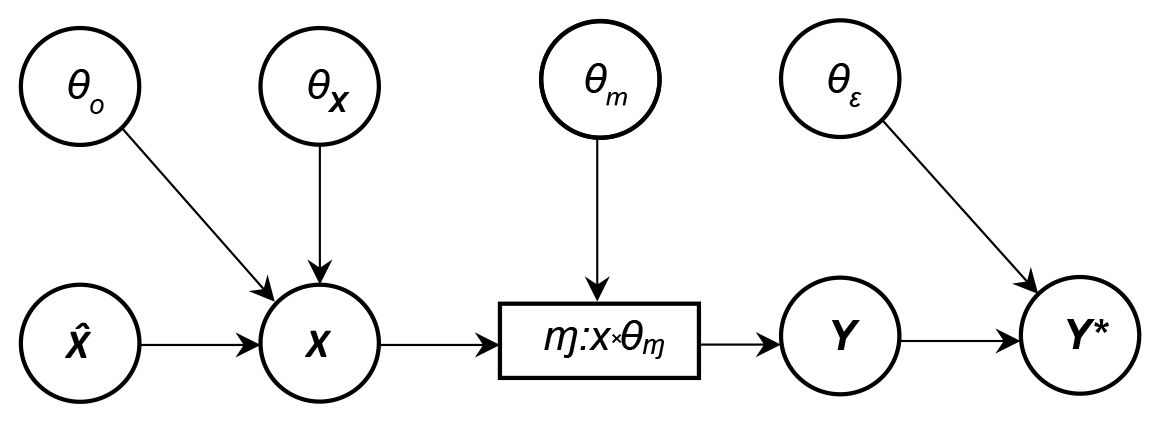
in which Θm refers to parameters of the model m, ΘX are parameters linked to the input X, Θε is the vector of the output-prediction error ε, and Θo is the vector associated with observation/measurement errors. More explicitly, to compute an overall joint probability distribution, we may have the following distributions:
-
is the distribution of Y when X takes the values x, and parameters θm∈Θm and a model m∈𝓜 are used to compute y;
-
f(x|θX,m) is the conditional distribution of X given the parameters θX∈ΘX and the model m. Note that each m defines which elements in X are to be considered in the analysis;
-
is a distribution of X given the observed values and the observation/measurement error parameters θo∈Θo;
-
additionally, one can consider ,m), which is a distribution of Y*, the future system's response, conditioned on the model output y and the output-prediction error vector θε∈Θε. The output-prediction error ε is the mismatch between the model predictions and non-observed system responses y*. ε is used to correct the imperfect model output y (Betz, 2017; Juang et al., 2019).
If, for example, the parameters Θm are poorly
known, a prior distribution π(θm|m) weighing each parameter
value θm for a model m is usually specified. A prior is a subjective
probability distribution quantified by expert judgement representing
uncertainty about the quantities prior to considering data (Raices-Cruz et al., 2022). When some measurements are available, such parameter values θm, or their
distributions π(θm|m), can be constrained by back-analysis
methods. Note that measurements ![]() form part of different sources of data
𝓓, i.e. . Back-analysis methods
include matching experimental measurements and calculated model outputs y
using different assumed values . Values for θm
can be calculated as follows (based on Liu et al., 2022):
form part of different sources of data
𝓓, i.e. . Back-analysis methods
include matching experimental measurements and calculated model outputs y
using different assumed values . Values for θm
can be calculated as follows (based on Liu et al., 2022):
The revision or updating of the prior π(θm|m) with
measurements ![]() to obtain a posterior distribution denoted is also an option in back analysis. The updating can be calculated
as follows (based on Juang et al., 2019; Liu et al., 2022):
to obtain a posterior distribution denoted is also an option in back analysis. The updating can be calculated
as follows (based on Juang et al., 2019; Liu et al., 2022):
where is a
likelihood function, i.e. a distribution that weighs ![]() given θm.
given θm.
Similarly, we can constrain any of the distributions above, e.g. , or to obtain and , respectively.
For a geohazard problem, it is often possible to specify several competing models, e.g. distinct geological models with diverse boundary conditions; see expression (2). If the available knowledge is insufficient to determine the best model, different models m can be considered. The respective overall output probability distribution is computed as (Betz, 2017; Juang et al., 2019)
In Eq. (6), is a distribution weighing each model m in 𝓜.
The various models 𝓜, their inputs X,
parameters Θ, outputs Y, and
experimental data ![]() can be coupled all together through a Bayesian network,
as has been suggested by Sankararaman and Mahadevan (2015) or Betz (2017).
One possible configuration of a network coupling some elements in
𝓜, X, Θ,
Y, and Y* is illustrated in Fig. 1.
can be coupled all together through a Bayesian network,
as has been suggested by Sankararaman and Mahadevan (2015) or Betz (2017).
One possible configuration of a network coupling some elements in
𝓜, X, Θ,
Y, and Y* is illustrated in Fig. 1.
The previous description of a general approach to UQ considers uncertainty
as that reflected in the analysts' incomplete knowledge about quantities or
events. In UQ, to measure or describe uncertainty, subjective probabilities
can be used and constrained using observations ![]() . It is also explicitly shown
that model outputs are conditional on observations
. It is also explicitly shown
that model outputs are conditional on observations ![]() made available and
models 𝓜 chosen by analysts. Analysts might also select
several parameters Θ and initial and boundary
conditions, BCm and ICm.
Based on the above description, in the following, we analyse some of the
challenges that arise when conducting UQ.
made available and
models 𝓜 chosen by analysts. Analysts might also select
several parameters Θ and initial and boundary
conditions, BCm and ICm.
Based on the above description, in the following, we analyse some of the
challenges that arise when conducting UQ.
As mentioned, back-analysis methods help constrain some elements in Θ. However, given the considerable number of parameters (see expressions 1–3) and data scarcity, constraining Θ is often only achieved in a limited fashion. Back-analysis is further challenged by the potential dependency among Θ or 𝓜 and between Θ and SGm, BCm, and ICm. We also note that back analysis, or, more specifically, inverse analysis, faces problems regarding non-identifiability, non-uniqueness, and instability. Non-identifiability occurs when some parameters do not drive changes in the inferred quantities. Non-uniqueness arises because more than one set of fitted or updated parameters may adequately reproduce observations. Instability in the solution arises from errors in observations and the non-linearity of models (Carrera and Neuman, 1986). Alternatively, in specifying a joint distribution f(x,θ) to be sampled, analysts may consider the use of e.g. Bayesian networks (Albert et al., 2022). However, under the usual circumstance of a lack of information, establishing such a joint distribution is challenging and requires that analysts encode many additional assumptions (e.g. prior distributions, likelihood functions, independence, linear relationships, normality, stationarity of the quantities and parameters considered); see e.g. Tang et al. (2020), Sun et al. (2021b), Albert et al. (2022), Pheulpin et al. (2022). A more conventional choice is that x or θ are specified using the maximum entropy principle (MEP), to specify the least biased distributions possible on the given information (Jaynes, 1957). Such distributions are subject to the system's physical constraints based on some available data. The information entropy of a probability distribution measures the amount of information contained in the distribution. The larger the entropy, the less information is provided by the distribution. Thus, by maximising the entropy over a suitable set of probability distributions, one finds the least informative distribution in the sense that it contains the least amount of information consistent with the system's constraints. Note that a distribution is sought over all the candidate distributions subject to a set of constraints. The MEP has been questioned since its validity and usefulness lie in the proper choice of physical constraints (Jaynes, 1957; Yano 2019). Doubts are also raised regarding the potential information loss when using the principle. Analysts usually strive to use all available knowledge and avoid unjustified information loss (Christakos, 1990; Flage et al., 2018).
Options to address the parametrisation challenge also include surrogate
models, parameter reduction, and model learning (e.g. Lu and Lermusiaux,
2021; Sun et al., 2021b; Albert et al., 2022; Degen et
al., 2022; Liu et al., 2022). Surrogate models are learnt to replace a
complicated model with an inexpensive and fast approximation. Parameter
reduction is achieved based on either principal component analysis or global
sensitivity analysis to determine which parameters significantly impact
model outputs and are essential to the analysis (Degen et al., 2022;
Wagener et al., 2022). Remarkably, versions of the model
learning option do not need any prior information about model equations
Em but require local verification of conservation
laws in the data ![]() (Lu and Lermusiaux, 2021). These approaches still require
large data sets sourced systematically, which is a frequent limitation in
geohazard assessments. More importantly, however, is that, like many models,
the credibility of unobserved surrogate model outputs can always be questioned, since,
for instance, records may miss crucial events (Woo, 2019). Models may also
fail to reproduce outputs caused by recorded abrupt changes (e.g. extreme
velocities of turbidity currents) (Alley, 2004). An additional point is the
issue of incomplete model response, which refers to a model not having a
solution for some combinations of the specified input quantities (Cardenas,
2019; van den Eijnden et al., 2022).
(Lu and Lermusiaux, 2021). These approaches still require
large data sets sourced systematically, which is a frequent limitation in
geohazard assessments. More importantly, however, is that, like many models,
the credibility of unobserved surrogate model outputs can always be questioned, since,
for instance, records may miss crucial events (Woo, 2019). Models may also
fail to reproduce outputs caused by recorded abrupt changes (e.g. extreme
velocities of turbidity currents) (Alley, 2004). An additional point is the
issue of incomplete model response, which refers to a model not having a
solution for some combinations of the specified input quantities (Cardenas,
2019; van den Eijnden et al., 2022).
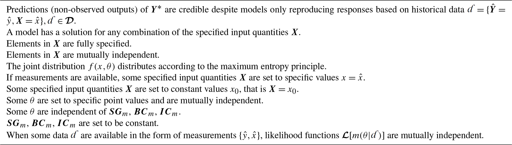
In bypassing the described challenges when quantifying uncertainty, simplifications are usually enforced, sometimes unjustifiably, in the form of assumptions, denoted here by Ą. The set Ą can include one or more of the assumptions listed in Table 1. Note that the set of assumptions can be increased with those assumptions imposed by using specific models 𝓜 (e.g. conservation of energy, momentum, or mass, Mohr–Coulomb's failure criterion).
From the previous section, we saw that it is very difficult in geohazard
assessments to meet data requirements for the ideal parameterisation of
models. Further, we have noted that, although fully parameterised models
could potentially be accurate at reproducing data from past events, these
may turn out to be inadequate for unobserved outputs. We also made explicit
that predictions are not only conditional on Θ but
possibly also on SGm, BCm, and
ICm; see expressions (1)–(7). Ultimately, assumptions
made also condition model outputs. More importantly, note that when only
some model input quantities or parameters can be updated using data ![]() , the
modelling will only reflect some aspects of the uncertainty involved. If the
above challenges remain unaddressed, UQ lacks credibility. To address such
challenges and provide increased credibility, clarifications and
reinterpretation of some fundamental concepts and practical simplifications
may be required, which are discussed in the following. Table 2 shows the
major challenges found and how they are addressed in related literature,
while in Table 3, some clarifications or considerations put forward by us
are displayed. The discussion in this section builds on previous analysis by
Aven and Pörn (1998), Apeland et al. (2002), Aven and
Kvaløy (2002), Nilsen and Aven (2003), Aven and Zio (2013), Khorsandi and
Aven (2017), and Aven (2019).
, the
modelling will only reflect some aspects of the uncertainty involved. If the
above challenges remain unaddressed, UQ lacks credibility. To address such
challenges and provide increased credibility, clarifications and
reinterpretation of some fundamental concepts and practical simplifications
may be required, which are discussed in the following. Table 2 shows the
major challenges found and how they are addressed in related literature,
while in Table 3, some clarifications or considerations put forward by us
are displayed. The discussion in this section builds on previous analysis by
Aven and Pörn (1998), Apeland et al. (2002), Aven and
Kvaløy (2002), Nilsen and Aven (2003), Aven and Zio (2013), Khorsandi and
Aven (2017), and Aven (2019).
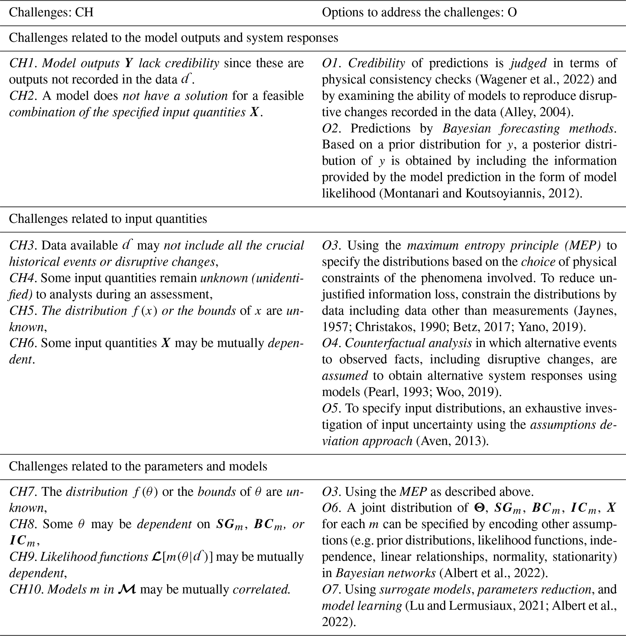
Table 3Some clarifications and considerations to address the challenges in UQ.
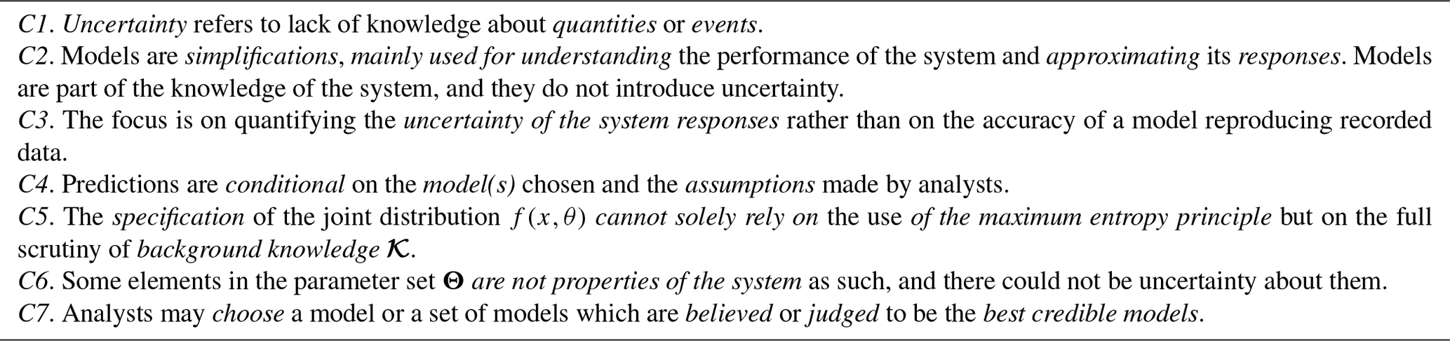
Among the clarifications, we consider a major conceptualisation suggested by
the literature, which is the definition of uncertainty. Uncertainty refers
to incomplete information or knowledge about a quantity or the occurrence of
an event (Society for Risk Analysis, 2018). In Table 3, we denote this
clarification as C1. Embracing this definition has some implications for
uncertainty quantification using geohazard models. We use these implications
to address the major complications and challenges. For instance, if
uncertainty is measured in terms of probability, one such implication is
that analysts are discouraged from using so-called frequentist
probabilities. We note that frequentist probabilities do not measure
uncertainty or lack of knowledge. Rather. such probabilities reflect
frequency ratios representing fluctuation or variation in the outcomes of
quantities. Frequentist probabilities are of limited use because these
assume that quantities vary in large populations of identical settings, a
condition which can be justified only for rather few geohazard quantities.
The often one-off nature of many geohazard features and the impossibility of
verifying or validating data by, e.g. a large number of repeated tests,
make it difficult to develop such probabilities. Thus, a more meaningful and
practical approach suggests to measure uncertainty by the use of
knowledge-based (also referred to as judgemental or subjective)
probabilities (Aven, 2019). A knowledge-based probability is an expression of
the degree of belief in the occurrence of an event or quantity by a person
assigning the probability conditional on the available knowledge
𝓚. Such knowledge 𝓚 includes not only
data in the form of measurements ![]() made available but also other data
sources in 𝓓. The models 𝓜 chosen for
the prediction and the modelling assumptions Ą made by
analysts are also part of 𝓚. Accordingly, to describe
uncertainty about quantities, probabilities are assigned based on
𝓚, and, therefore, those probabilities are conditional on
𝓚. In the previous section, we have made evident the
conditional nature of the uncertainty quantification (i.e. the
probabilities) on measured data
made available but also other data
sources in 𝓓. The models 𝓜 chosen for
the prediction and the modelling assumptions Ą made by
analysts are also part of 𝓚. Accordingly, to describe
uncertainty about quantities, probabilities are assigned based on
𝓚, and, therefore, those probabilities are conditional on
𝓚. In the previous section, we have made evident the
conditional nature of the uncertainty quantification (i.e. the
probabilities) on measured data ![]() and models 𝓜 and wrote
the expression f(y|x, Θ, 𝓓, 𝓜) for the overall output probability
distribution (see Eq. 6). If assumptions Ą are also
acknowledged as a conditional argument of the uncertainty quantification, we
write more explicitly f(y|x, Θ, 𝓓, 𝓜, Ą) or
equivalently . We can
therefore write
and models 𝓜 and wrote
the expression f(y|x, Θ, 𝓓, 𝓜) for the overall output probability
distribution (see Eq. 6). If assumptions Ą are also
acknowledged as a conditional argument of the uncertainty quantification, we
write more explicitly f(y|x, Θ, 𝓓, 𝓜, Ą) or
equivalently . We can
therefore write
The meaning of this expression is explained next. If, in a specific case, we would write , it means that 𝓓 summarises all the knowledge that analysts have to calculate y given (realised or known) x and θ. Accordingly, the full expression in Eq. (8) implies that to calculate y, and given the knowledge of x and θ, the background knowledge includes 𝓓, 𝓜, and Ą. Note that 𝓚 can also be formed by observations, justifications, rationales, and arguments; thus, Eq. (8) can be further detailed to include these aspects of 𝓚. Structured methods exist to assign knowledge-based probabilities (see, e.g. Apeland et al., 2002; Aven, 2019). Here we should note, however, that since models form part of the available background knowledge 𝓚, models can also inform these knowledge-based probability assignments. It follows that, based on knowledge-based input probabilities, an overall output probability distribution calculated using models is also subjective or knowledge-based (Jaynes, 1957). Some of the implications of using knowledge-based probabilities are described throughout this section.
According to the left column in Table 2, the focus of the challenges relates to the model outputs, more specifically predictions (CH1 and CH2), input quantities (CH3–CH6), parameters (CH7–CH9), and models (CH10). We recall that uncertainty quantification helps determine the system's response uncertainty based on specified input quantities. Accordingly, an assessment focuses on the potential system's responses. The focus is often on uncertainty about future non-observed responses Y*, which are approximated by the model output Y, considering some specified input quantities X. We recall that Y* and X* are quantities that are unknown at the time of the analysis but will take some value in the future and possibly become known. Thus, during an assessment, Y* and X* are the uncertain quantities of the system since we have incomplete knowledge about Y* and X*. Accordingly, the output-prediction error ε, the mismatch between the model prediction values y, and the non-observed system's response values y* can only be specified based on the scrutiny of 𝓚.
There is another consequence of considering the definition of uncertainty put forward in C1, which links uncertainty solely to quantities or events. The consequence is that models, as such, are not to be linked to uncertainty. Models are merely mathematical artefacts. Models, per se, do not introduce uncertainty, but they are likely inaccurate. Accordingly, another major distinction is to be set in place. We recall that models, by definition, are simplifications, approximations of the system being analysed. They express or are part of the knowledge of the system. Models should therefore be solely used for understanding the performance of the system rather than for illusory perfect predictions. In Table 3, we denote the latter clarification as C2.
Regarding the challenges CH1 and CH2, we should note that geohazard analysts are often more interested in predictions rather than known system outputs. For instance, predictions are usually required to be calculated for input values not contained in the validation data. We consider that predictions are those model outputs not observed or recorded in the data, i.e. extrapolations out of the range of values covered by observations. Thus, the focus is on quantifying the uncertainty of the system's responses rather than on the accuracy of a model reproducing recorded data. This is the clarification C3 in Table 3. Considering this, models are yet to provide accuracy in reproducing observed outputs but, more importantly, afford credibility in predictions. Such credibility is to be assessed mainly in terms of judgements, since conventional validation cannot be conducted using non-observed outputs. Recall that model accuracy usually relates to comparing model outputs with experimental measurements (Roy and Oberkampf, 2011; Aven and Zio, 2013) and is the basis for validating models. Regarding the credibility of predictions, Wagener et al. (2022) have reported that such credibility can be mainly judged in terms of the physical consistency of the predictions. Such consistency is judged by checks rejecting physically impossible representations of the system. The credibility of predictions may also include the verification of the ability of models to accurately reproduce disruptive changes recorded in the data (Alley, 2004). However, as we have made explicit in the previous section, model predictions are conditional on a considerable number of critical assumptions and choices made by analysts (see Table 1 and clarification C4 in Table 3). Therefore, predictions can only be as good as the quality of the assumptions made. The assumptions could be wrong, and the examination of the impact of these deviations on the predictions must be assessed. To provide credibility of predictions, such assumptions and choices should be justified and scrutinised; see option O5 in Table 2. Option O5 addresses the challenge CH1; however, when conducting UQ, O5 has a major role when investigating input uncertainty, which is discussed next.
A critical task in UQ is the quantification of input uncertainty. Input
uncertainty may originate when crucial historical events or disruptive
changes are missing in the records (CH3). Some critical input quantities may
also remain unidentified to analysts during an assessment (CH4). Analysts can
unintendedly fail to identify relevant elements in X* due
to insufficiencies in data or limitations of existing models. For example,
during many assessments, trigger factors that could bring a soil mass to
failure could remain unknown to analysts (e.g. Hunt et al., 2013; Clare et
al., 2016; Leynaud et al., 2017; Casalbore et al., 2020). UQ requires
simulating sampled values from X, and elements in X can be mutually
dependent. However, the joint distribution of X, namely f(x), is often also unknown. This is the challenge CH6. Considering the potential
challenges CH3 to CH6, to specify f(x), we cannot solely rely on using the maximum
entropy principle (MEP). The MEP may fail to advance an exhaustive
uncertainty quantification in the input, e.g. by missing relevant values
not recorded in the measured data. This would undermine the quality of
predictions and, therefore, uncertainty quantification. Recall that the MEP
suggests using the least informative distribution among candidate
distributions constrained solely on measurements. Using counterfactual
analysis, as described in Table 2, is an option. However, the counterfactual
analysis will also fail to provide quality predictions, since this analysis
focuses on counterfactuals (alternative events to observed facts ![]() , ) and little on the overall knowledge available
𝓚. Note that the knowledge 𝓚 about the
system includes, e.g. the assumptions made in the UQ, such as those shown
in Table 1. Further note that such assumptions relate not only to data but
also to input quantities, modelling, and predictions. Thus, it appears that
the examination of these assumptions should be at the core of UQ in
geohazard assessments, as suggested in Table 2, option O5. The risk assessment
of deviations from assumptions was originally suggested by Aven (2013) and
exemplified by Khorsandi and Aven (2017). An assumption deviation risk
assessment evaluates different deviations, their associated probabilities of
occurrence, and the effect of the deviations. A major distinctive feature of
the assumption deviation risk assessment approach is the evaluation of the
credibility of the knowledge 𝓚 supporting the assumptions
made. Another feature of this approach is questioning the justifications
supporting the potential for deviations. The examination of
𝓚 can be achieved by assessing the justifications for the
assumptions made, the amount and relevance of data or information, the
degree of agreement among experts, and the extent to which the phenomena
involved are understood and can be modelled accurately. Justifications might
be in the form of direct evidence becoming available, indirect evidence from
other observable quantities, supported by modelling results, or possibly
inferred by assessments of deviations of assumptions. This approach is
succinctly demonstrated in the following section. Accordingly, we suggest
specifying f(x) in terms of knowledge-based probabilities in conjunction with
investigating input uncertainty using the assumptions deviation approach.
This is identified as consideration C5 in Table 3.
, ) and little on the overall knowledge available
𝓚. Note that the knowledge 𝓚 about the
system includes, e.g. the assumptions made in the UQ, such as those shown
in Table 1. Further note that such assumptions relate not only to data but
also to input quantities, modelling, and predictions. Thus, it appears that
the examination of these assumptions should be at the core of UQ in
geohazard assessments, as suggested in Table 2, option O5. The risk assessment
of deviations from assumptions was originally suggested by Aven (2013) and
exemplified by Khorsandi and Aven (2017). An assumption deviation risk
assessment evaluates different deviations, their associated probabilities of
occurrence, and the effect of the deviations. A major distinctive feature of
the assumption deviation risk assessment approach is the evaluation of the
credibility of the knowledge 𝓚 supporting the assumptions
made. Another feature of this approach is questioning the justifications
supporting the potential for deviations. The examination of
𝓚 can be achieved by assessing the justifications for the
assumptions made, the amount and relevance of data or information, the
degree of agreement among experts, and the extent to which the phenomena
involved are understood and can be modelled accurately. Justifications might
be in the form of direct evidence becoming available, indirect evidence from
other observable quantities, supported by modelling results, or possibly
inferred by assessments of deviations of assumptions. This approach is
succinctly demonstrated in the following section. Accordingly, we suggest
specifying f(x) in terms of knowledge-based probabilities in conjunction with
investigating input uncertainty using the assumptions deviation approach.
This is identified as consideration C5 in Table 3.
Another point to consider is that when uncertainty is measured in terms of knowledge-based probabilities, analysts should be aware of what conditionality means. If, for example, a quantity X2 is conditional on a quantity X1, this implies that increased knowledge about X1 will change the uncertainty about X2. The expression that denotes this is conventionally written as X2|X1. Analysts may exploit this interpretation when specifying, e.g. the joint distribution f(x,θ). For example, when increased knowledge about a quantity X1 will not result in increased knowledge about another quantity X2, analysts may simplify the analysis according to the scrutiny of 𝓚, meaning that a distribution to be specified may reduce to according to probability theory. Apeland et al. (2002) have illustrated how conditionality in the setting of knowledge-based probabilities can inform the specification of a joint distribution.
The parameterisation problem, which involves the challenges CH7 to CH9 in Table 2, warrants exhaustive consideration. Addressing these challenges also requires some reinterpretation. To start, note that parameters are coefficients determining specific functions among a family of potential functions modelling the system. Those parameters constrain a model's output. Recall that y, as realisations of Y, are the model output when X takes the values x, and some parameters θ∈Θ, and models m∈𝓜 are used. Thus, as shown in the previous section, any output y is conditional on θ, and so is the uncertainty attached to y*. We may also distinguish two types of parameters. We may have parameters associated with a property of the system. Other parameters exist that are merely artefacts in the models and are not properties of the system. As suggested, if uncertainty can solely be attached to events or quantities, we may say that parameters that are not properties of the system are not to be linked to any uncertainty. This is identified as clarification C6 in Table 3. For example, analysts may consider that the parameters not being part of the system as such are those linked to the output-prediction error ε, the vector associated with observation/measurement errors Θo, and the overall attached hyperparameters linked to probability distributions (including priors, likelihood functions). Analysts may consider the latter parameters as modelling artefacts, so it is questionable to attach uncertainty to them. Thus, focused on the uncertainty of the system responses rather than model inaccuracies, uncertainty is to be assigned to those parameters that represent physical quantities. Fixed single values can be assigned to those parameters that are not properties of the system. To help identify those parameters to which some uncertainty can be linked, we can scrutinise, e.g. the physical nature of these. In fixing parameters to a single value, we can still make use of back-analysis procedures, as mentioned previously. Analysts may have some additional basis to specify parameter values when the background knowledge available 𝓚 is scrutinised. 𝓚 can be examined to verify that not only data measurements but other sources of data, models, and assumptions made strongly support a specific parameter value. Based on this interpretation, setting the values of the parameters that are not properties of the system to a single value reduces the complications in quantifying uncertainty considerably. It also follows that analysts are encouraged to make explicit that model outputs are conditional on these fixed parameters, and on the model or models chosen, as we have shown in the previous section. The latter also leads us to argue that the focus of UQ is on the uncertainty of the system response rather than the inaccuracies of the models. This implies in a practical sense that in geohazard assessments, when parameters are clearly differentiated from specified input quantities, and models providing the most credible predictions are chosen, uncertainty quantification can then proceed. This parsimonious modelling approach is identified as consideration C7 in Table 3. This latter consideration addresses, to an extent, the challenge CH10.
In the following section, we further illustrate the above discussion by analysing a documented case in which UQ in a geohazard assessment was informed by modelling using sampling procedures.
To further describe the proposed considerations, we analyse a case reported in the specialised literature. The case deals with the quantification of uncertainty of geological structures, namely uncertainty about the subsurface stratigraphic configuration. Conditions in the subsurface are highly variable, whereas site investigations only provide sparse measurements. Consequently, subsurface models are usually inaccurate. At a given location, subsurface conditions are unknown until accurately measured. Soil investigation at all locations is usually impractical and uneconomical, and point-to-point condition variation cannot be known (Vanmarcke, 1984). Such uncertainty means significant engineering and environmental risk to, e.g. infrastructure built on the surface. One way to quantify this uncertainty is by calculating the probability of every possible configuration of the geological structures (Tacher et al., 2006; Thiele et al., 2016; Pakyuz-Charrier et al., 2018). Sampling procedures for UQ are helpful in this undertaking. We use an analysis and information from Zhao et al. (2021), which refer to a site located in the Central Business District, Perth, Western Australia, where six boreholes were executed. The case has been selected taking into account its simplicity to illustrate the points of this paper, but at the same time, it provides details to allow some discussion. Figure 2 displays the system being analysed.
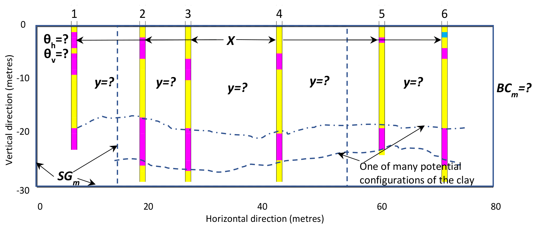
Figure 2Borehole logs in colours and longitudinal section reported by Zhao et al. (2021) located in the Central Business District, Perth, Western Australia. The records correspond to information on six boreholes. Three types of materials are revealed by the boreholes, including sand (yellow), clay (magenta), and gravel (blue).
In the system under consideration, a particular material type to be found in a non-bored point, a portion of terrain not penetrated during soil investigation, is unknown and thus uncertain. The goal is to compute the probability of encountering a given type of soil at these points. Zhao et al. (2021) focus on calculating the probabilities of encountering clay in the subsurface. The approach advocated was a sampling procedure to generate many plausible configurations of the geological structures and evaluate their probabilities. In a non-penetrated point in the ground, to calculate the probability of encountering a given type of soil c, p(y=c), Zhao et al. (2021) used a function that depends on two correlation parameters, namely the horizontal and vertical scale of fluctuation θh and θv. Note that spatial processes and their properties are conventionally assumed as spatially correlated. Such spatial variation may presumably be characterised by correlation functions, which depend on a scale of fluctuation parameter. The scale of fluctuation measures the distance within which points are significantly correlated (Vanmarcke, 1984). Equation (9) describes the basic components of the model chosen by Zhao et al. (2021) (specific details are given in the Appendix to this paper) as follows:
where X is the collection of all specified quantities at borehole points sx which can take values x from the set {sand, clay, gravel}, according to the setting in Fig. 2. Y is the collection of all model outputs with values y at non-borehole points sy. Probabilities p(y=c) are computed based on the sampling of the values y and x, and a chosen model using the parameters θh=11.1 and θv=4.1 m, θh, θv∈Θm. Using the maximum likelihood method, the parameters were determined based on the borehole data revealed at the site. In determining parameters, the sampling from uniform and mutually independent distributions of θh and θv was the procedure advocated. The system is further described by a set of equations Em (a correlation function and a probability function), the spatial domain geometry sgm (a terrain block of 30×80 m), and the boundary conditions bcm (the conditions at the borders). More details are given in the Appendix to this paper. Since this system is not considered time-dependent, the initial conditions ICm were not specified.
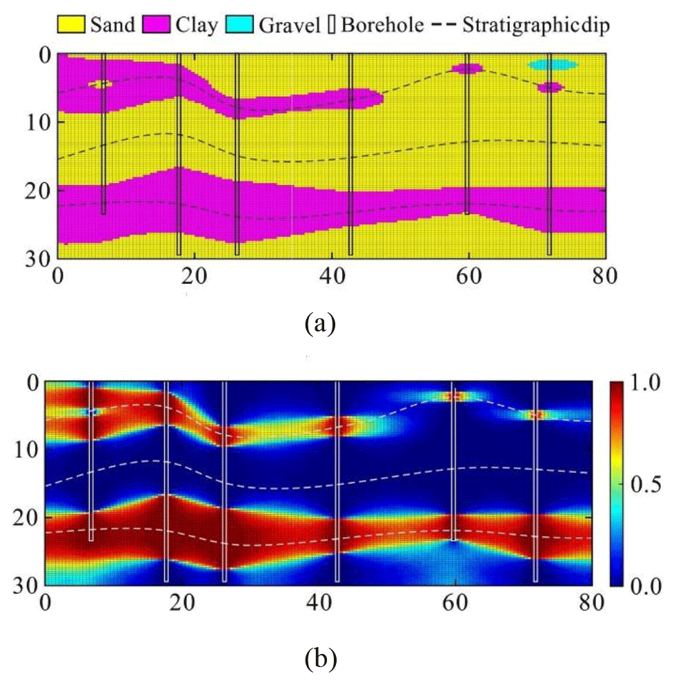
Figure 3Zhao et al. (2021) findings shown in their Fig. 9. (a) Most probable stratigraphic configuration. (b) Spatial distribution of the probability of the existence of clay. Reprinted from Engineering Geology, 238, Zhao et al. (2021), Probabilistic characterisation of subsurface stratigraphic configuration with modified random field approach, p. 106138, © 2021, with permission from the COPYRIGHT OWNER: Elsevier. Distances in metres.
The summary results reported by Zhao et al. (2021) are shown in Fig. 3. In Fig. 3, the most probable stratigraphic configuration, along with the spatial distribution of the probability of the existence of clay, is displayed. The authors focused on this sensitive material, which likely represents a risk to the infrastructure built on the surface.
Zhao et al. (2021) stated that “characterisation results of the stratigraphic configuration and its uncertainty are consistent with the intuition and the state of knowledge on site characterisation”. Next, throughout Zhao et al.'s (2021) analysis, the following assumptions were enforced (Table 4), although these were not explicitly disclosed by the authors.

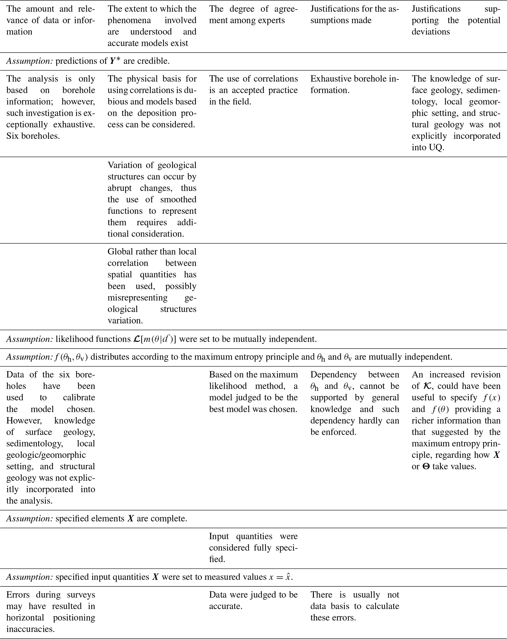
Unfortunately, the authors did not report enough details on how the majority of these assumptions are justified. We should note, however, that providing these justifications was not the objective of their research. Yet, here we analyse how assumptions can be justified by scrutinising 𝓚 and using some elements of the assumption deviation approach described in the previous section. Table 5 summarises the analysis conducted and only reflects the most relevant observations and reservations we identified. Accordingly, the information in Table 5 may not be exhaustive but is still useful for the desired illustration. Table 5 displays some of our observations related to the credibility of the knowledge 𝓚. The examination of 𝓚 is achieved by assessing the amount and relevance of data or information, the extent to which the phenomena involved are understood and can be modelled accurately, the degree of agreement among experts, and the justifications for the assumptions made. Observations regarding the justifications for potential deviations from assumptions also form part of the analysis.
Not surprisingly, the observations in our analysis concentrate on the predictions' credibility. Recall that UQ focuses on the system's response, approximated by model predictions (considerations C2 and C3 in Table 3). For example, although using correlations is an accepted practice and a practical simplification, correlation functions appear counterintuitive to model geological structures or domains. Further, correlation functions do not help much in understanding the system (consideration C2 in Table 3). Recall that such structures are mainly disjoint domains linked to a finite set of possible categorical quantities (masses of soil or rock) rather than continuous quantities. Next, the variation of such structures can occur by abrupt changes in materials; thus, the use of smoothed correlation functions to represent them requires additional consideration. Moreover, the physical basis of the correlation functions is not clear, and physical models based on deposition processes may be suggested (e.g. Catuneanu et al., 2009). We should note a potential justification for the deviation from the assumption regarding the credibility of predictions. This is because knowledge from additional sources such as surface geology, sedimentology, local geomorphic setting, and structural geology was not explicitly taken into account in quantifying uncertainty. The revision of this knowledge can contribute to reducing the probability of deviation in predictions. Based on the observations in Table 5, we can conclude that there is potential to improve the credibility of predictions.
The choices made by Zhao et al. (2021) regarding the use of parameters with fixed values together with the choice for a single best model can be highlighted. These choices illustrate the points raised in considerations C6 and C7 (Table 3). The maximum likelihood method supported these choices; a back-analysis method focused on matching measurements and calculated model outputs using different assumed values for θh and θv. We highlight that a model judged to be the best model was chosen. This includes the specification of a particular spatial domain geometry in SGm. Investigating the impact of the variation of SGm was considered unnecessary. There was no need to specify several competing models, which is in line with our consideration labelled as C7 in this paper.
Zhao et al. (2021) investigated the joint distribution f(x), which was sampled to calculate probabilities. However, someone can suggest that the joint distribution f(x,θ,sgm,bcm) could have been produced. Nevertheless, we can argue that establishing such a joint distribution is challenging and requires, in many instances, that analysts encode many additional assumptions (e.g. prior distributions, likelihood functions, independence, linear relationships, normality, stationarity of the quantities and parameters considered).
Table 5Examination of supporting knowledge 𝓚 and justifications for the potential deviation of assumptions.
A more crucial observation derived from the analysis of potential deviations of assumptions might considerably impact the credibility of predictions. This observation comes from revisiting the knowledge sources of Zhao et al.'s (2021) analysis, available from https://australiangeomechanics.org/downloads/ (last access: 29 June 2022). Another type of sensitive material was revealed by other soundings in the area, more specifically, silt. Depending on the revision of 𝓚, this fourth suspected material could be analysed in an extended uncertainty quantification of the system. Note that the specified input quantities X were originally assumed to take values x from the set {sand, clay, gravel}. Such an assumption was based on the records of six boreholes which were believed to be accurate. The latter illustrates the relevance of consideration C5 in Table 3.
Another choice by Zhao et al. (2021) is that they disregarded the possibility of incorporating measurement errors of the borehole data into the UQ, probably because these data were judged to be accurate. We recall in this respect that these errors reflect the inaccuracy of the measurements rather than the uncertainty about the system. As stated for consideration C6 (Table 3), we can hardly justify attaching uncertainty to measurement error parameters, since measurement errors are not a property of the system. The same can be said for the parameters θh and θv, which are not properties of the system. Note that their physical basis is questioned. We should note, however, that assuming global coefficients for the parameters θh and θv is an established practice (Vanmarcke, 1984; Lloret-Cabot et al., 2014; Juang et al., 2019). It can be pointed out that uncertainty quantification in this kind of system is, to an extent, sensitive to the choice of scale of fluctuation values (Vanmarcke, 1984). It can also be argued that using a global rather than local correlation between spatial quantities can misrepresent geological structure variation. Accordingly, further examination of the existing knowledge 𝓚 justifies some assessment of the impact of assuming a local rather than global scale of fluctuation.
Overall, the Zhao et al. (2021) analysis is, to an extent, based on the previously suggested definition of uncertainty; see the consideration C1 in Table 3.
We should stress that Zhao et al.'s (2021) uncertainty quantification refers specifically to the ground model described at the beginning of this section. In other words, the probabilities displayed in Fig. 3b are conditional on the parameters chosen (θh=11.1 and θv=4.1 m), the model selected (described by Eqs. 9, A1 and A2 in the Appendix to this paper), the specified spatial domain geometry sgm (a terrain block of 30×80 m), and ultimately the assumptions made (listed in Table 4). This information is to be reported explicitly to the users of the results. This reflects the clarification C4 in Table 3.
Regarding the consideration of subjective probabilities, there has been some
agreement on their use in this kind of UQ since Vanmarcke (1984). However,
the use of knowledge-based probabilities in the extension described here is
recommended, given the illustrated implications to advance UQ (as discussed
in the previous section and stated in consideration C5). For example,
increased examination of 𝓚 might have resulted in using a
more informative distribution f(θh,θv) than the
uniform distribution. The increased examination of 𝓚 might
have led to different values for θh and θv, and a different model. Recall that the selection of the model and
determination of parameters were based on the maximum likelihood method,
which only uses measured data ![]() .
.
In our analysis of Zhao's et al. (2021) assessment, the examination of supporting knowledge 𝓚 resulted essentially in
-
judging the credibility of predictions;
-
providing justifications for assessing assumption deviations by considering the modelling of a fourth material;
-
considering additional data other than the borehole records, such as surface geology, sedimentology, local geomorphic setting, and structural geology;
-
analysing the possibility of distinct geological models with diverse spatial domain geometry and local correlations; and
-
ultimately, further examining the existing 𝓚.
In this paper, we have discussed challenges in uncertainty quantification (UQ) for geohazard assessments. Beyond the parameterisation problem, the challenges include assessing the quality of predictions required in the assessments, quantifying uncertainty in the input quantities, and considering the impact of choices and assumptions made by analysts. Such challenges arise from the commonplace situation of limited data and the one-off nature of geohazard features. If these challenges are kept unaddressed, UQ lacks credibility. Here, we have formulated seven considerations that may contribute to providing increased credibility in the quantifications. For example, we proposed understanding uncertainty as lack of knowledge, a condition that can only be attributed to quantities or events. Another consideration is that the focus of the quantification should be more on the uncertainty of the system response rather than the accuracy of the models used in the quantification. We drew attention to the clarification that models, in geohazard assessments, are simplifications used for predictions approximating the system's responses. We have also considered that since uncertainty is only to be linked to the properties of the system, models do not introduce uncertainty. Inaccurate models can, however, produce poor predictions and such models should be rejected. Then, an increased examination of background knowledge will be required to quantify uncertainty credibly. We also put forward that there could not be uncertainty about those elements in the parameter set that are not properties of the system. The latter also has pragmatic implications, including how the many parameters in a geohazard system could be constrained in a geohazard assessment.
We went into detail to show that predictions, and in turn UQ, are conditional on the model(s) chosen together with the assumptions made by analysts. We identified limitations of measured data to support the assessment of the quality of predictions. Accordingly, we have proposed that the quality of UQ needs to be judged based also on some additional crucial tasks. Such tasks include the exhaustive scrutiny of the knowledge coupled with the assessment of deviations of those assumptions made in the analysis.
Key to enacting the proposed clarifications and simplifications is the full consideration of knowledge-based probability. Considering this type of probability will help overcome the identified limitations of the maximum entropy principle or counterfactual analysis to quantify uncertainty in input quantities. We have exposed that the latter approaches are prone to produce unexhausted uncertainty quantification due to their reliance on measured data, which can miss crucial events or overlook relevant input quantities.
In this Appendix, the necessary details of the original analysis made by Zhao et al. (2021) are given. The following are the basic equations Em used by these authors:
where X is the collection of all specified quantities at borehole points, which take values x. Y is the collection of all outputs at non-borehole points with values y. ρxy is the value of correlation between a quantity value x at a penetrated point sx∈Sx and the value y at a non-penetrated point sy∈Sy. is the horizontal distance between points sx and sy, while |sxsy is the vertical one. θh and θv are the horizontal and vertical scales of fluctuation, respectively. Each material class considered is associated exclusively with an element in the set of integers . p(y=c) is the probability of encountering a type of material c in a point sy. Such probability is initially approximated using Eq. (A1). More accurate probabilities are computed based on the repeated sampling of the joint distribution f(x,y), which was approximated using Eq. (A1). Equation (A1), described in short, approximates probabilities as the ratio of the sum of correlation values, calculated for a penetrated point in the set Sx and the set of non-penetrated points Sy for a given material c, to the sum of correlation values for all points and all materials.
Based on data collected at borehole locations, the selection of the type of
correlation function and the scales of fluctuation took place using the
maximum likelihood method. The authors considered three types of correlation
functions, namely squared exponential, single exponential, and second-order
Markov. In this case, the likelihood function represents the likelihood of
observing ![]() at borehole locations, given the spatial correlation structure
θm. The squared exponential function yielded the maximum
likelihood when the horizontal and vertical scales of fluctuation were set
to 11.1 and 4.1 m, respectively. Hence, the squared exponential
function correlation, whose expression is Eq. (A2) in this Appendix, was
selected. Equations (A3) and (A4) correspond to the single exponential and the
second-order Markov functions, respectively.
at borehole locations, given the spatial correlation structure
θm. The squared exponential function yielded the maximum
likelihood when the horizontal and vertical scales of fluctuation were set
to 11.1 and 4.1 m, respectively. Hence, the squared exponential
function correlation, whose expression is Eq. (A2) in this Appendix, was
selected. Equations (A3) and (A4) correspond to the single exponential and the
second-order Markov functions, respectively.
No data sets were used in this article.
ICC: conceptualisation, methodology, writing (original draft preparation), investigation, and validation. TA: investigation, supervision, and writing (reviewing and editing). RG: investigation, supervision, and writing (reviewing and editing).
The contact author has declared that none of the authors has any competing interests.
Publisher's note: Copernicus Publications remains neutral with regard to jurisdictional claims in published maps and institutional affiliations.
The authors are very grateful to the reviewers, who provided valuable and useful suggestions.
This research is funded by ARCEx partners and the Research Council of Norway (grant no. 228107).
This paper was edited by Dan Lu and David Ham and reviewed by Anthony Gruber and one anonymous referee.
Albert, C. G., Callies, U., and von Toussaint, U.: A Bayesian approach to the estimation of parameters and their interdependencies in environmental modeling, Entropy, 24, 231, https://doi.org/10.3390/e24020231, 2022.
Alley, R. B.: Abrupt climate change, Sci. Am., 291, 62–69, https://doi.org/10.1126/science.1081056, 2004.
Apeland, S., Aven, T., and Nilsen, T.: Quantifying uncertainty under a predictive, epistemic approach to risk analysis, Reliab. Eng. Syst. Saf., 75, 93–102, https://doi.org/10.1016/S0951-8320(01)00122-3, 2002.
Aven, T.: On the need for restricting the probabilistic analysis in risk assessments to variability, Risk Anal., 30, 354–360, https://doi.org/10.1111/j.1539-6924.2009.01314.x, 2010.
Aven, T.: Practical implications of the new risk perspectives, Reliab. Eng. Syst. Saf., 115, 136–145, https://doi.org/10.1016/j.ress.2013.02.020, 2013.
Aven, T.: The science of risk analysis: Foundation and practice, Routledge, London, https://doi.org/10.4324/9780429029189, 2019.
Aven, T. and Kvaløy, J. T.: Implementing the Bayesian paradigm in risk analysis, Reliab. Eng. Syst. Saf., 78, 195–201, https://doi.org/10.1016/S0951-8320(02)00161-8, 2002.
Aven, T. and Pörn, K.: Expressing and interpreting the results of quantitative risk analyses, Review and discussion, Reliab. Eng. Syst. Saf., 61, 3–10, https://doi.org/10.1016/S0951-8320(97)00060-4, 1998.
Aven, T. and Zio, E.: Model output uncertainty in risk assessment, Int. J. Perform. Eng., 29, 475–486, https://doi.org/10.23940/ijpe.13.5.p475.mag, 2013.
Betz, W.: Bayesian inference of engineering models, Doctoral dissertation, Technische Universität München, 2017.
Brown, G. W.: Monte Carlo methods, Modern Mathematics for the Engineers, 279–303, McGraw-Hill, New York, 1956.
Cardenas, I.: On the use of Bayesian networks as a meta-modelling approach to analyse uncertainties in slope stability analysis, Georisk, 13, 53–65, https://doi.org/10.1080/17499518.2018.1498524, 2019.
Carrera, J. and Neuman, S.: Estimation of aquifer parameters under transient and steady state conditions: 2. Uniqueness, stability, and solution algorithms, Water Resour. Res., 22, 211–227, https://doi.org/10.1029/WR022i002p00211, 1986.
Casalbore, D., Passeri, F., Tommasi, P., Verrucci, L., Bosman, A., Romagnoli, C., and Chiocci, F. L.: Small-scale slope instability on the submarine flanks of insular volcanoes: the case-study of the Sciara del Fuoco slope (Stromboli), Int. J. Earth Sci., 109, 2643–2658, https://doi.org/10.1007/s00531-020-01853-5, 2020.
Catuneanu, O., Abreu, V., Bhattacharya, J. P., Blum, M. D., Dalrymple, R. W., Eriksson, P. G., Fielding, C. R., Fisher, W. L., Galloway, W. E., Gibling, M. R., Giles, K. A., Holbrook, J. M., Jordan, R., Kendall, C. G. St. C., Macurda, B., Martinsen, O. J., Miall, A. D., Neal, J. E., Nummedal, D., Pomar, L., Posamentier, H. W., Pratt, B. R., Sarg, J. F., Shanley, K. W., Steel, R. J., Strasser, A., Tucker, M. E., and Winker, C.: Towards the standardisation of sequence stratigraphy, Earth-Sci. Rev., 92, 1–33, https://doi.org/10.1016/j.earscirev.2008.10.003, 2009.
Chow, Y. K., Li, S., and Koh, C. G.: A particle method for simulation of submarine landslides and mudflows, Paper presented at the 29th International Ocean and Polar Engineering Conference, 16–21 June, Honolulu, Hawaii, USA, ISOPE-I-19-594, 2019.
Christakos, G.: A Bayesian/maximum-entropy view to the spatial estimation problem, Math. Geol., 22, 763–777, https://doi.org/10.1007/BF00890661, 1990.
Clare, M. A., Clarke, J. H., Talling, P. J., Cartigny, M. J., and Pratomo, D. G.: Preconditioning and triggering of offshore slope failures and turbidity currents revealed by most detailed monitoring yet at a fjord-head delta, Earth Planet. Sc. Lett., 450, 208–220, https://doi.org/10.1016/j.epsl.2016.06.021, 2016.
Degen, D., Veroy, K., Scheck-Wenderoth, M., and Wellmann, F.: Crustal-scale thermal models: Revisiting the influence of deep boundary conditions, Environ. Earth Sci., 81, 1–16, https://doi.org/10.1007/s12665-022-10202-5, 2022.
Dubois, D.: Possibility theory and statistical reasoning, Comput. Stat. Data Anal., 51, 47–69, https://doi.org/10.1016/j.csda.2006.04.015, 2006.
Ferson, S. and Ginzburg, L. R.: Different methods are needed to propagate ignorance and variability, Reliab. Eng. Syst. Saf., 54, 133–144, https://doi.org/10.1016/S0951-8320(96)00071-3, 1996.
Flage, R., Baraldi, P., Zio, E., and Aven, T.: Probability and possibility-based representations of uncertainty in fault tree analysis, Risk Anal., 33, 121–133, https://doi.org/10.1111/j.1539-6924.2012.01873.x, 2013.
Flage, R., Aven, T., and Berner, C. L.: A comparison between a probability bounds analysis and a subjective probability approach to express epistemic uncertainties in a risk assessment context – A simple illustrative example, Reliab. Eng. Syst. Saf., 169, 1–10, https://doi.org/10.1016/j.ress.2017.07.016, 2018.
Gray, A., Ferson, S., Kreinovich, V., and Patelli, E.: Distribution-free risk analysis, Int. J. Approx. Reason., 146, 133–156, https://doi.org/10.1016/j.ijar.2022.04.001, 2022a.
Gray, A., Wimbush, A., de Angelis, M., Hristov, P. O., Calleja, D., Miralles-Dolz, E., and Rocchetta, R.: From inference to design: A comprehensive framework for uncertainty quantification in engineering with limited information, Mech. Syst. Signal Process., 165, 108210, https://doi.org/10.1016/j.ymssp.2021.108210, 2022b.
Hastings, W. K.: Monte Carlo sampling methods using Markov chains and their applications, Biometrika, 87, 97–109, https://doi.org/10.2307/2334940, 1970.
Helton, J. C. and Oberkampf, W. L.: Alternative representations of epistemic uncertainty, Reliab. Eng. Syst. Saf., 1, 1–10, https://doi.org/10.1016/j.ress.2011.02.013, 2004.
Huang, L., Cheng, Y. M., Li, L., and Yu, S. Reliability and failure mechanism of a slope with non-stationarity and rotated transverse anisotropy in undrained soil strength, Comput. Geotech., 132, 103970, https://doi.org/10.1016/j.compgeo.2020.103970, 2021.
Hunt, J. E., Wynn, R. B., Talling, P. J., and Masson, D. G.: Frequency and timing of landslide-triggered turbidity currents within the Agadir Basin, offshore NW Africa: Are there associations with climate change, sea level change and slope sedimentation rates?, Mar. Geol., 346, 274–291, https://doi.org/10.1016/j.margeo.2013.09.004, 2013.
Jaynes, E. T.: Information theory and statistical mechanics, Phys. Rev., 106, 620, https://doi.org/10.1103/PhysRev.106.620, 1957.
Juang, C. H., Zhang, J., Shen, M., and Hu, J.: Probabilistic methods for unified treatment of geotechnical and geological uncertainties in a geotechnical analysis, Eng. Geol, 249, 148–161, https://doi.org/10.1016/j.enggeo.2018.12.010, 2019.
Khorsandi, J. and Aven, T.: Incorporating assumption deviation risk in quantitative risk assessments: A semi-quantitative approach, Reliab. Eng. Syst. Saf., 163, 22–32, https://doi.org/10.1016/j.ress.2017.01.018, 2017.
Leynaud, D., Mulder, T., Hanquiez, V., Gonthier, E., and Régert, A.: Sediment failure types, preconditions and triggering factors in the Gulf of Cadiz, Landslides, 14, 233–248, https://doi.org/10.1007/s10346-015-0674-2, 2017.
Liu, Y., Ren, W., Liu, C., Cai, S., and Xu, W.: Displacement-based back-analysis frameworks for soil parameters of a slope: Using frequentist inference and Bayesian inference, Int. J. Geomech., 22, 04022026, https://doi.org/10.1061/(ASCE)GM.1943-5622.0002318, 2022.
Lloret-Cabot. M., Fenton, G. A., and Hicks, M. A.: On the estimation of scale of fluctuation in geostatistics, Georisk, 8, 129–140, https://doi.org/10.1080/17499518.2013.871189, 2014.
Lu, P. and Lermusiaux, P. F.: Bayesian learning of stochastic dynamical models, Phys. D, 427, 133003, https://doi.org/10.1016/j.physd.2021.133003, 2021.
Luo, L., Liang, X., Ma, B., and Zhou, H.: A karst networks generation model based on the Anisotropic Fast Marching Algorithm, J. Hydrol., 126507, https://doi.org/10.1016/j.jhydrol.2021.126507, 2021.
Metropolis, N. and Ulam, S.: The Monte Carlo method, J. Am. Stat. A., 44, 335–341, https://doi.org/10.1080/01621459.1949.10483310, 1949.
Montanari, A. and Koutsoyiannis, D.: A blueprint for process-based modeling of uncertain hydrological systems, Water Resour. Res., 48, W09555, https://doi.org/10.1029/2011WR011412, 2012.
Nilsen, T. and Aven, T.: Models and model uncertainty in the context of risk analysis, Reliab. Eng. Syst. Saf., 79, 309–317, https://doi.org/10.1016/S0951-8320(02)00239-9, 2003.
Pakyuz-Charrier, E., Lindsay, M., Ogarko, V., Giraud, J., and Jessell, M.: Monte Carlo simulation for uncertainty estimation on structural data in implicit 3-D geological modeling, a guide for disturbance distribution selection and parameterization, Solid Earth, 9, 385–402, https://doi.org/10.5194/se-9-385-2018, 2018.
Pearl, J.: Comment: graphical models, causality and intervention, Statist. Sci., 8, 266–269, 1993.
Pheulpin, L., Bertrand, N., and Bacchi, V.: Uncertainty quantification and global sensitivity analysis with dependent inputs parameters: Application to a basic 2D-hydraulic model, LHB, 108, 2015265, https://doi.org/10.1080/27678490.2021.2015265, 2022.
Raíces-Cruz, I., Troffaes, M. C., and Sahlin, U.: A suggestion for the quantification of precise and bounded probability to quantify epistemic uncertainty in scientific assessments, Risk Anal., 42, 239–253, https://doi.org/10.1111/risa.13871, 2022.
Rodríguez-Ochoa, R., Nadim, F., Cepeda, J. M., Hicks, M. A., and Liu, Z.: Hazard analysis of seismic submarine slope instability, Georisk, 9, 128–147, https://doi.org/10.1080/17499518.2015.1051546, 2015.
Roy, C. J. and Oberkampf, W. L.: A comprehensive framework for verification, validation, and uncertainty quantification in scientific computing, Comput. Methods Appl. Mech. Eng., 200, 2131–2144, https://doi.org/10.1016/j.cma.2011.03.016, 2011.
Sankararaman, S. and Mahadevan, S.: Integration of model verification, validation, and calibration for uncertainty quantification in engineering systems, Reliab. Eng. Syst. Saf., 138, 194–209, https://doi.org/10.1016/j.ress.2015.01.023, 2015.
Shafer, G.: A mathematical theory of evidence, in: A mathematical theory of evidence, Princeton university press, 1976.
Shortridge, J., Aven, T., and Guikema, S.: Risk assessment under deep uncertainty: A methodological comparison, Reliab. Eng. Syst. Saf., 159, 12–23, https://doi.org/10.1016/j.ress.2016.10.017, 2017.
Society for Risk Analysis: Society for Risk Analysis glossary, https://www.sra.org/wp-content/uploads/2020/04/SRA-Glossary-FINAL.pdf (last access: 25 June 2021), 2018.
Sun, X., Zeng, P., Li, T., Wang, S., Jimenez, R., Feng, X., and Xu, Q.: From probabilistic back analyses to probabilistic run-out predictions of landslides: A case study of Heifangtai terrace, Gansu Province, China, Eng. Geol, 280, 105950, https://doi.org/10.1016/j.enggeo.2020.105950, 2021a.
Sun, X., Zeng, X., Wu, J., and Wang, D.: A Two-stage Bayesian data-driven method to improve model prediction, Water Resour. Res., 57, e2021WR030436, https://doi.org/10.1029/2021WR030436, 2021b.
Tacher, L., Pomian-Srzednicki, I., and Parriaux, A.: Geological uncertainties associated with 3-D subsurface models, Comput. Geosci., 32, 212–221, https://doi.org/10.1016/j.cageo.2005.06.010, 2006.
Tang, X. S., Wang, M. X., and Li, D. Q.: Modeling multivariate cross-correlated geotechnical random fields using vine copulas for slope reliability analysis, Comput. Geotech., 127, 103784, https://doi.org/10.1016/j.compgeo.2020.103784, 2020.
Thiele, S. T., Jessell, M. W., Lindsay, M., Wellmann, J. F., and Pakyuz-Charrier, E.: The topology of geology 2: Topological uncertainty, J. Struct. Geol., 91, 74–87, https://doi.org/10.1016/j.jsg.2016.08.010, 2016.
Ulam, S. M.: Monte Carlo calculations in problems of mathematical physics, Modern Mathematics for the Engineers, 261–281, McGraw-Hill, New York, 1961.
Uzielli, M. and Lacasse, S.: Scenario-based probabilistic estimation of direct loss for geohazards, Georisk, 1, 142–154, https://doi.org/10.1080/17499510701636581, 2007.
van den Eijnden, A. P., Schweckendiek, T., and Hicks, M. A.: Metamodelling for geotechnical reliability analysis with noisy and incomplete models, Georisk, 16, 518–535, https://doi.org/10.1080/17499518.2021.1952611, 2022.
Vanmarcke, E. H.: Random fields: Analysis and synthesis, The MIT Press, Cambridge, MA, 1984.
Vanneste, M., Løvholt, F., Issler, D., Liu, Z., Boylan, N., and Kim, J.: A novel quasi-3D landslide dynamics model: from theory to applications and risk assessment, Paper presented at the Offshore Technology Conference, 6–9 May, Houston, Texas, OTC-29363-MS, https://doi.org/10.4043/29363-MS, 2019.
Wagener, T., Reinecke, R., and Pianosi, F.: On the evaluation of climate change impact models, Wiley Interdiscip, Rev. Clim. Change, e772, https://doi.org/10.1002/wcc.772, 2022.
Wellmann, J. F. and Regenauer-Lieb, K.: Uncertainties have a meaning: Information entropy as a quality measure for 3-D geological models, Tectonophysics, 526, 207–216, https://doi.org/10.1016/j.tecto.2011.05.001, 2012.
Woo, G.: Downward counterfactual search for extreme events, Front. Earth Sci., 7, 340, https://doi.org/10.3389/feart.2019.00340, 2019.
Yano, J. I.: What is the Maximum Entropy Principle? Comments on “Statistical theory on the functional form of cloud particle size distributions”, J. Atmos. Sci., 76, 3955–3960, https://doi.org/10.1175/JAS-D-18-0223.1, 2019.
Zadeh, L. A.: Probability measures of fuzzy events, J. Math. Anal. Appl., 23, 421–427, https://doi.org/10.1016/0022-247X(68)90078-4, 1968.
Zhao, C., Gong, W., Li, T., Juang, C. H., Tang, H., and Wang, H.: Probabilistic characterisation of subsurface stratigraphic configuration with modified random field approach, Eng. Geol, 288, 106138, https://doi.org/10.1016/j.enggeo.2021.106138, 2021.