the Creative Commons Attribution 4.0 License.
the Creative Commons Attribution 4.0 License.
 | 20 Mar 2023
UKESM1.1: development and evaluation of an updated configuration of the UK Earth System Model
Jane P. Mulcahy
Colin G. Jones
Steven T. Rumbold
Till Kuhlbrodt
Andrea J. Dittus
Edward W. Blockley
Andrew Yool
Jeremy Walton
Catherine Hardacre
Timothy Andrews
Alejandro Bodas-Salcedo
Marc Stringer
Lee de Mora
Phil Harris
Richard Hill
Doug Kelley
Eddy Robertson
Yongming Tang
Many Coupled Model Intercomparison Project phase 6 (CMIP6) models have exhibited a substantial cold bias in the global mean surface temperature (GMST) in the latter part of the 20th century. An overly strong negative aerosol forcing has been suggested as a leading contributor to this bias. An updated configuration of UK Earth System Model (UKESM) version 1, UKESM1.1, has been developed with the aim of reducing the historical cold bias in this model. Changes implemented include an improved representation of SO2 dry deposition, along with several other smaller modifications to the aerosol scheme and a retuning of some uncertain parameters of the fully coupled Earth system model. The Diagnostic, Evaluation and Characterization of Klima (DECK) experiments, a six-member historical ensemble and a subset of future scenario simulations are completed. In addition, the total anthropogenic effective radiative forcing (ERF), its components and the effective and transient climate sensitivities are also computed. The UKESM1.1 preindustrial climate is warmer than UKESM1 by up to 0.75 K, and a significant improvement in the historical GMST record is simulated, with the magnitude of the cold bias reduced by over 50 %. The warmer climate increases ocean heat uptake in the Northern Hemisphere oceans and reduces Arctic sea ice, which is in better agreement with observations. Changes to the aerosol and related cloud properties are a driver of the improved GMST simulation despite only a modest reduction in the magnitude of the negative aerosol ERF (which increases by +0.08 W m−2). The total anthropogenic ERF increases from 1.76 W m−2 in UKESM1 to 1.84 W m−2 in UKESM1.1. The effective climate sensitivity (5.27 K) and transient climate response (2.64 K) remain largely unchanged from UKESM1 (5.36 and 2.76 K respectively).
- Article
(16449 KB) - Full-text XML
-
Supplement
(8584 KB) - BibTeX
- EndNote


The works published in this journal are distributed under the Creative Commons Attribution 4.0 License. This license does not affect the Crown copyright work, which is re-usable under the Open Government Licence (OGL). The Creative Commons Attribution 4.0 License and the OGL are interoperable and do not conflict with, reduce or limit each other.
© Crown copyright 2020
The ability of a global climate model (GCM) to accurately simulate the historical climate is generally regarded as being an important indicator of the model's potential skill in simulating future climate. In particular, the historical global mean surface temperature is a widely used metric in assessing the performance of global climate models, despite this not necessarily directly translating to skilful future climate projections (Kiehl, 2007). A number of modelling centres employ various tuning practices to achieve good agreement with the observed historical temperature record during the model development cycle (Mauritsen and Roeckner, 2020; Hourdin et al., 2017; Schmidt et al., 2017), while others treat it as an emergent model property (Senior et al., 2020). Notwithstanding such practices, many models participating in the sixth Coupled Model Intercomparison Project (CMIP6) have a significant cold bias in the historical global mean surface temperature through the latter half of the 20th century (Flynn and Mauritsen, 2020). An overly strong aerosol forcing has been suggested to be a leading candidate responsible for this bias, which is consistent with the increasing anthropogenic aerosol emissions during this period (Flynn and Mauritsen, 2020; Dittus et al., 2020; Andrews et al., 2020). In particular, anthropogenic emissions of sulfur dioxide (SO2), a precursor to sulfate (SO4) aerosol, was the predominant source of anthropogenic aerosols during this time. Sulfate aerosol directly scatters incoming shortwave solar radiation and can also influence the cloud albedo and lifetime by acting as efficient cloud condensation nuclei. After 1980, with the widespread implementation of clean air legislation, SO2 emissions steadily declined, and the climate has subsequently warmed in response to greenhouse gas emissions.
UK Earth System Model version 1 (UKESM1) has a particularly large cold bias peaking in the 1970–1980 period, with a negative bias approaching 0.5 K (Sellar et al., 2019). Investigations by Hardacre et al. (2021) highlight a significant positive bias in the surface concentration of SO2 in UKESM1 at measurement sites across the historically large emission source regions of Europe and northeastern USA. Interestingly, a low bias in surface SO4 concentrations is found in the same regions (Mulcahy et al., 2020; Hardacre et al., 2021). More generally, Earth system models (ESMs) with more complex chemistry and aerosol schemes have a larger cold bias in CMIP6 than their physical model counterparts (Zhang et al., 2021). A strong correlation is found between the anthropogenic sulfate burden and surface temperature change over the historical period, further strengthening the argument for the role of an overly strong sulfate aerosol forcing in these models (Zhang et al., 2021).
Given the likely strong contribution of aerosol to the historical surface temperature bias, a number of key questions arise regarding the simulation of SO2, the pathways leading to sulfate aerosol and associated aerosol–climate interactions in UKESM1. Specifically, are the emissions of anthropogenic SO2 too high in the CMIP6 forcing dataset (McDuffie et al., 2020; Aas et al., 2019), or are the sinks of SO2 realistically simulated in the model? With respect to the latter, we refer to wet and dry deposition in addition to loss via the chemical oxidation of SO2 to sulfate aerosol. If sink processes are too low, then the atmospheric residence time of SO2 will be too long, resulting in excess SO2 being transported away from industrial source regions and being oxidised to form aerosol in more pristine remote regions which are more susceptible to aerosol forcing (Carslaw et al., 2013). Evidence suggests that a large fraction (up to 50 %) of emitted anthropogenic SO2 is deposited within 200 to 300 km of emission sources, with 30 %–35 % dry deposited and 10 %–15 % oxidised to SO4 (Smith and Jeffrey, 1975; Wys et al., 1978). In coarse-resolution climate models like UKESM1, this is the equivalent to two or three model grid boxes, and so accurately representing these subgrid processes is challenging in GCMs.
Hardacre et al. (2021) examine the impact of an updated parameterisation for the dry deposition of SO2 on the surface SO2 concentration bias in UKESM1. The new parameterisation considers whether the surface vegetation is wet or dry when calculating the surface resistance to species uptake. Due to the high solubility of SO2, the wetter and more humid it is at the surface, the higher the uptake of SO2. The new parameterisation leads to a significant improvement (of the order of 50 %) in the positive SO2 bias against ground-based observations in the above study. Despite this improvement in the simulation of surface SO2, the reductions in SO2 close to the emission sources further degrade the pre-existing low bias in SO4 aerosol (Hardacre et al., 2021; Mulcahy et al., 2020), and so model process deficiencies in the oxidation of SO2 to SO4 also likely exist. Interestingly, Hardacre et al. (2021) show a larger relative reduction in surface SO2 and SO4 remote from the source (e.g. over the North Atlantic region) than over the source regions, supporting the above assertion that excess SO2 close to source regions drives remote aerosol loading and subsequent aerosol forcing.
In this paper, we document and characterise a new science configuration of the UKESM model, which we refer to as UKESM1.1. While the revised SO2 dry deposition parameterisation comprises the main science development in UKESM1.1, we also incorporate a number of smaller science changes resulting from the extensive evaluation of the UKESM1 model (e.g. Sellar et al., 2019; Mulcahy et al., 2020; Yool et al., 2019; Robson et al., 2020). In addition, we revise some of the specific tunings applied to the coupled aspects of UKESM, as outlined in Sellar et al. (2019). In Sect. 2 we describe the UKESM1.1 science configuration, detailing all model changes and motivations for such changes, while Sect. 3 details the model simulations conducted as part of this study. The impact of the new configuration on a number of key climate-based metrics is assessed in Sect. 4. We focus our evaluation on the fully coupled historical simulations and compare the present-day UKESM1.1 climate to its predecessor, UKESM1, and a wide range of observations where available. We then assess the impact of the new model on the anthropogenic forcing, the transient and effective climate sensitivities. Finally, we compare the future climate response to UKESM1.
The UKESM1 model is described in detail in Sellar et al. (2019), and so we provide only an overview of its components here. UKESM1 comprises the global coupled atmosphere–ocean climate model, HadGEM3-GC3.1 (Williams et al., 2017), along with additional Earth system components, which are important because of their feedbacks on the climate system. These include the simulation of the uptake of carbon and nitrogen in marine and terrestrial ecosystems and the interactive representation of trace gas and aerosol composition changes in addition to their interactions within the full Earth system.
The physical atmosphere component (including aerosol) of UKESM1 (and HadGEM3-GC3.1) is the Global Atmosphere 7.1 (GA7.1) science configuration of the Unified Model (Walters et al., 2019; Mulcahy et al., 2018) and has a horizontal resolution of approximately 135 km (1.25∘ × 1.875∘) and 85 vertical levels, with a terrain-following hybrid height coordinate, reaching up to 85 km. Aerosols and trace gas chemistry are simulated in UKESM1 using the stratospheric–tropospheric configuration of the United Kingdom Chemistry and Aerosol (UKCA) model (Archibald et al., 2020) which is coupled to the two-moment modal version of the Global Model of Aerosol Processes, GLOMAP-mode (Mulcahy et al., 2020, 2018). The aerosol model component, and changes implemented in this work are described in more detail below.
In the ocean, UKESM1 uses the low-resolution version (1∘; Kuhlbrodt et al., 2018) of the Nucleus for European Modelling of the Ocean (NEMO; Storkey et al., 2018) with 75 vertical levels. Sea ice is simulated using the Los Alamos sea ice model (CICE; Ridley et al., 2018). A small correction to the coupled sea ice heat fluxes in NEMO is applied here. This corrects an inconsistent use of the sea ice fraction in the calculation of the sea ice grid box mean values (used in the CICE component) from the sea ice area mean values (used in the atmosphere component).
The land surface component uses the Joint UK Land Environment Simulator (JULES) model (Best et al., 2011; Clark et al., 2011) and shares the same latitude–longitude grid as the atmosphere. Surface and subsurface runoff is transported to the ocean using the TRIP river routing scheme (Total Runoff Integrating Pathways; Oki and Sud, 1998). Terrestrial biogeochemistry is simulated in UKESM1 by coupling JULES to the dynamic vegetation model, TRIFFID (Top-down Representation of Interactive Foliage and Flora Including Dynamics; Cox, 2001) and the RothC soil carbon model (Rothamsted carbon model; Coleman and Jenkinson, 1999). Updates made to these schemes for inclusion into UKESM1 are described in Sellar et al. (2019). Noteworthy developments included the extension of plant functional types to better distinguish between evergreen and deciduous plants and between tropical and temperate evergreen plants, the inclusion of a nitrogen scheme, which limits terrestrial carbon uptake, and extensions to the representation of land use change.
Marine biogeochemistry is simulated using the Model of Ecosystem Dynamics nutrient Utilisation, Sequestration and Acidification (MEDUSA; Yool et al., 2013, 2021). MEDUSA is a medium-complexity plankton ecosystem model representing the biogeochemical cycles of nitrogen, silicon and iron nutrients, as well as carbon, alkalinity and dissolved oxygen.
2.1 Aerosol developments
The GLOMAP-mode aerosol scheme represents the emissions, atmospheric evolution and deposition of sea salt, sulfate, black carbon and organic carbon species. Full details of the aerosol scheme, as implemented in UKESM1, and a detailed evaluation of the historical aerosol simulation, as run for CMIP6, are given in Mulcahy et al. (2020).
A number of developments to the SO2 dry deposition scheme are implemented here. These are described in detail in Hardacre et al. (2021), so we only briefly outline them here. The dry deposition scheme in UKCA follows that of Wesely (1989). This uses a resistance-based approach to calculate the dry deposition velocity, vd, as follows:
where ra represents the aerodynamic resistance, rb is the quasi-laminar sublayer resistance, and rc represents the surface resistance. The dry deposition developments in this work apply to the surface resistance term, rc, which is sensitive to the individual surface properties and surrounding climatic conditions. For non-vegetated surfaces (e.g. open water, bare soil or snow-covered surfaces), rc is set at a suitable global constant. Over vegetated surfaces, rc is calculated as a function of the stomatal resistance (Rstom), the canopy cuticle resistance (Rcut) and the soil resistance (Rsoil). Rsoil and Rcut are defined for the 13 fractional land cover types in the model. In UKESM1, the calculation of Rcut and Rsoil is neither dependent on whether the underlying vegetation is wet or dry, nor does it depend on the near-surface climate conditions. Given the high solubility of SO2, this is expected to lead to rc values which are too high, and subsequently, the dry deposition of this gas will be underestimated (Hardacre et al., 2021). In the updated scheme, the modelled precipitation is used to determine the degree of surface wetness. Rcut and Rsoil for SO2 are then parameterised as a function of the surface wetness, near-surface relative humidity and temperature, following Erisman and Baldocchi (1994); Erisman et al. (1994). Therefore, rather than having a fixed rc value for each vegetation type, rc now varies as a function of the near-surface conditions, with rc being at its minimum when a surface grid box is classified as wet.
In addition, while analysing the UKESM1 SO2 dry deposition scheme, an error in the value of rc over ocean surfaces was uncovered. This value had been incorrectly set to 148.9 s m−1 during the development of UKESM1, instead of 10 s m−1, as set in the physical model (HadGEM3-GC3.1) and used in Mulcahy et al. (2018). Numerous studies (e.g. Garland, 1977; Erisman et al., 1994; Zhang et al., 2003) indicate the resistance to SO2 deposition over the open ocean is minimal, with reported values ranging from 0.004 to 20 s m−1. Therefore, in addition to introducing the extension to SO2 dry deposition over the land surfaces as described above, we assign a value of 1 s m−1 to open-water surface fractions, noting that this is different to the value used in GC3.1.
Table 1Summary of the dimethyl sulfide (DMS) chemical reactions in UKESM1 and UKESM1.1.
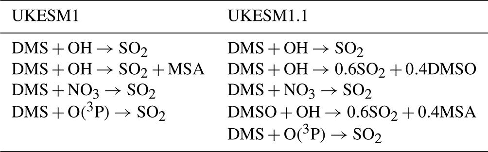
Finally, a number of additional bugs in the aerosol model, which were uncovered after the freeze of UKESM1, have been corrected. The tropospheric chemistry of dimethyl sulfide (DMS) in the full stratosphere–troposphere version of UKCA was previously simplified to offset some of the additional computational cost of extending the chemistry in the stratosphere (Archibald et al., 2020). This resulted in a different set of chemical reactions to that in the previously used troposphere-only scheme (O'Connor et al., 2014) and the offline oxidant scheme used in GC3.1 (Mulcahy et al., 2020). Currently, in the gas-phase, DMS is oxidised by OH via an abstraction and addition pathway. The addition pathway neglects the formation of the intermediary product, dimethyl sulfoxide (DMSO), despite this being a transported tracer which undergoes wet and dry deposition, in the stratosphere–troposphere chemistry scheme. In UKESM1.1, the DMS chemistry is updated, as shown in Table 1, and is now consistent with GC3.1. The DMS chemistry remains a simple scheme; Revell et al. (2019) investigated the impacts of more complex DMS chemistry on SO4 aerosol production and found a notable impact on cloud droplet number concentrations in the Southern Ocean.
A correction to the updating of sulfuric acid (H2SO4) first reported in Ranjithkumar et al. (2021) is also applied. In GLOMAP-mode, the chemistry and aerosol time step is currently 1 h, but microphysical processes such as condensation, nucleation and coagulation occur on a shorter 4 min substep. The concentration of H2SO4, required for both condensation and nucleation, should also have been updated on the shorter time step but was only being produced on the longer time step in UKESM1. This led to an erroneously high number concentration of small particles produced from the binary homogeneous nucleation of sulfuric acid. This is corrected here, with the primary effect being a reduction in the nucleation mode of SO4 aerosol in the free troposphere.
A further correction was applied to the UKCA-Activate scheme (West et al., 2014), which parameterises the activation of aerosol particles into cloud droplets. In this scheme, the activated cloud droplet number concentration per metre cubed is replicated upward from cloud base in contiguous clouds. This should rather be in units of numbers per kilogram of air to correctly replicate the expansion of a rising air parcel with height. Correcting this bug reduces Nd in contiguous clouds, in particular for deep clouds.
2.2 Tuning of the coupled Earth system
We revisit some of the tuned parameters of the fully coupled system previously described in Kuhlbrodt et al. (2018) and Sellar et al. (2019). For the purposes of this tuning we make use of the atmosphere-only, UKESM1 Atmospheric Model Intercomparison Project (AMIP) configuration in most cases (apart from the tuned sea ice model parameters as described in Sect. 2.2.1), which allows us to more easily evaluate the impact of the tuning on present-day metrics for which more observations are available. As already mentioned above, the tuning of the UKESM1 configuration was done in a preindustrial climate only. Here, numerous AMIP simulations were conducted, with the parameters of interest independently adjusted and outputs evaluated against observations. A summary of the final tuned values in UKESM1 and UKESM1.1 are provided in Table 2.
Table 2Summary of tuned parameters in UKESM1 and UKESM1.1.
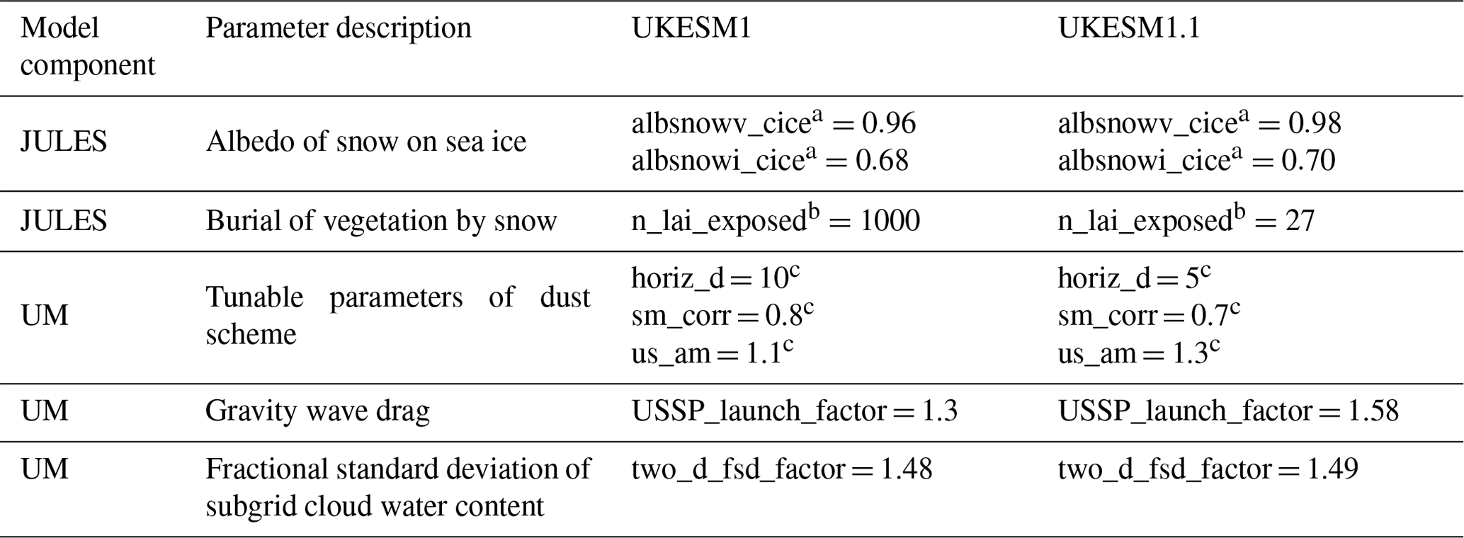
a Visible and near-infrared albedos for snow on sea ice. b n_lai_exposed was changed for grasses and temperate broadleaf evergreen trees only. c Multiplicative-scale factors for the horizontal dust emission flux, the frictional velocity and soil moisture.
2.2.1 Albedo of snow on sea ice
In UKESM1, the albedo of snow on sea ice was decreased by 2 percentage points (Kuhlbrodt et al., 2018) to compensate for the deficient transport of warm Atlantic Ocean water into the Arctic Ocean in the lower-resolution ocean model. As we will later show, the SO2 changes generally warm the climate, in particular the Northern Hemisphere, and so we revert to the original value as set in the 0.25∘ model (HadGEM3-GC3.1-MM; Williams et al., 2017). The new and old values are specified in Table 2.
2.2.2 Burial of vegetation by snow
Another parameter that required tuning in the fully coupled ESM is the parameter, n_lai_exposed, which controls the degree to which vegetation is buried by snow. This was tuned in UKESM1 to correct for biases in the net surface shortwave (SW) radiation introduced when the interactive vegetation scheme was coupled to the physical model, GC3.1. When evaluated with present-day simulations, however, this tuning appears to lead to an excessive burial by snow and results in a net positive bias in the DJF (December–February) top-of-atmosphere (TOA) clear-sky outgoing SW radiation between 30 and 60∘ N (see Table 2 in Sellar et al., 2019). As the climate warms with rising CO2 concentrations, the excessively bright snow-covered grassland is replaced by darker forests. This positive feedback was found to increase the effective climate sensitivity in UKESM1 (Andrews et al., 2019). In UKESM1.1, n_lai_exposed for grasses and temperate broadleaf evergreen trees has been reduced from 1000 to 27 in order to reduce the extent of the snow burial of vegetation. The retuning of n_lai_exposed reduces the SW snow metric from above to below the observed range (see Table S1 in the Supplement). We note that Sellar et al. (2019) refer to this target range as being a crude representation of the true observational uncertainty. The UKESM1.1 performance for this metric is therefore as acceptable as UKESM1 and remains an improvement over the untuned model.
2.2.3 Dust
While the total aerosol optical depth (AOD) in UKESM1 compares generally well against observations, the mineral dust optical depth (DOD) is biased low (Mulcahy et al., 2020; Checa-Garcia et al., 2021). This is despite UKESM1 having larger dust emissions and comparable dust burdens compared to other CMIP6 models (Checa-Garcia et al., 2021).
One of the key factors influencing the disparity in dust between models is the particle size distribution. UKESM1 has a significant portion of its dust in the super-coarse particle size range. Such particles have a very short atmospheric lifetime and are not optically efficient, resulting in lower DOD compared to other models which have a larger fraction of dust in the accumulation mode. As reported in Sellar et al. (2019), the mineral dust scheme (Woodward, 2001, 2011) used in UKESM1 is highly sensitive to a number of parameters, including the vegetation distribution, influencing the bare soil fraction available for dust erosion, soil moisture and wind speed. In UKESM1, all of these elements are dynamic and evolve in response to the changing climatic conditions. Sellar et al. (2019) documents the three tuned parameters in UKESM1. Here we revise this dust tuning with the aim of increasing the DOD to improve the agreement with ground-based and satellite AOD measurements. Table 2 specifies the original parameter values in UKESM1 and the revised values in UKESM1.1. The revised tuned parameters lead to a slight reduction in global dust emissions of approximately 10 %, but the DOD is nearly doubled, while the total AOD is increased by 10 %–20 % (see Fig. S1). These changes are consistent with a reduction in the horiz_d parameter, which scales the total emission, and a shift in the dust size distribution to the smaller sizes as a result of changes to the parameters controlling the sensitivity of soil moisture (sm_corr) and frictional velocity (us_am). AOD increases are found primarily over the Sahara, Saudi Arabia and India, with much smaller increases simulated over Australia (see Fig. S1). The spatial distribution of the AOD is also in much better agreement with satellite retrievals of AOD from the MODIS (Moderate Resolution Imaging Spectroradiometer) and MISR (Multi-angle Imaging SpectroRadiometer) sensors, in particular over the Sahara desert and in the dust outflow regions west of Africa. However, positive AOD biases over India are exacerbated. With more dust particles residing in the accumulation mode, the potential lifetime of dust will increase, with implications for the dust transport and subsequent iron deposition to the ocean in the fully coupled system. The scaling factor converting dust deposition into iron addition to the ocean was therefore also tuned so that approximately 2.6 Gmol Fe yr−1 is added to the ocean by this process (Yool et al., 2013). The same approach was used during the development and tuning of UKESM1 (Sellar et al., 2019).
2.2.4 Quasi-biennial oscillation
The parameter (USSP_launch_factor) controlling the flux of subgrid gravity waves generated by non-orographic sources is sensitive to both model resolution and science configuration and generally requires retuning when changing model resolution or implementing new science (Walters et al., 2014). This retuning was erroneously neglected during the development of UKESM1, which subsequently inherited the value of USSP_launch_factor used in the higher-resolution physical model. As a consequence, the period of the tropical quasi-biennial oscillation (QBO) was found to be too low in UKESM1 when compared against reanalyses (Richter et al., 2020). This has implications for the Southern Hemisphere climate in particular. The flux of the parameterised convectively generated wave momentum needs to be tuned in accordance with the model's wind and thermal structure. To do this, we tune the launched gravity waves such that the QBO gives a reasonable comparison with reanalyses.
UKESM1 has a mean QBO period of 43 months compared with 28 months in the Modern-Era Retrospective analysis for Research and Applications (MERRA) reanalysis (see Fig. S2). In UKESM1.1, the mean QBO period is 28 months, which is in agreement with the MERRA reanalysis (Fig. S2).
2.2.5 Radiation balance
Once the science configuration of UKESM1.1, including the model component tunings described above, was finalised, a final tuning of the net radiation at the TOA was required to ensure that it is in balance. This retuning was done on a fully coupled preindustrial control simulation and was achieved by adjusting the two_d_fsd_factor parameter. This parameter scales the fractional standard deviation of the cloud water content in a grid box, as seen by the radiation scheme (Hill et al., 2015). Increasing the parameter value translates to a greater assumed subgrid inhomogeneity of the grid box mean cloud water and thus a less reflective cloud (and vice versa, for decreased values of this parameter), although only a small retuning of this parameter – from a value of 1.48 to 1.49 – was required here.
All model simulations assessed in this study follow the CMIP6 protocols outlined in Eyring et al. (2016). While the tuning of the modified parameters discussed above predominantly made use of the computationally faster atmosphere-only (AMIP) simulations, the development of UKESM1.1 was conducted in a fully coupled preindustrial (PI) climate driven by 1850 forcing conditions. A continuously evolving PI control climate state was simulated, with each change added incrementally. Once the final configuration of the model was frozen, a further 462 simulated years of the PI control (piControl) were run. A six-member historical ensemble was run with transient forcing from 1850 to 2014. The initial conditions (including atmosphere, ocean, sea ice and land states) for each member of the ensemble were branched from the piControl and were equally spaced at 40 years apart. In addition, the full set of Diagnostic, Evaluation and Characterization of Klima (DECK) experiments (Eyring et al., 2016) were conducted. These comprise a preindustrial control simulation (piControl) already discussed above, an abrupt-4×CO2 simulation in which the PI climate is forced by an abrupt quadrupling of CO2 and run for 150 years, a 1pctCO2 experiment in which a 150-year PI simulation is forced by a 1 % per year increase in CO2 and, finally, an AMIP simulation covering the period 1979 to 2014. In the AMIP simulation, the sea surface temperature and sea ice conditions are prescribed from observations (Durack and Taylor, 2017), while other atmosphere–ocean and atmosphere–land coupled variables are replaced with climatological forcing data taken from the first member of the historical ensemble. Specifically, in UKESM, the prescribed fields include transient annual mean vegetation fractions, a monthly mean climatology of the leaf area index, seawater DMS and sea surface chlorophyll concentrations and an annual mean climatology of canopy height.
An atmosphere-only version of the piControl, piClim-control, was also used to determine the anthropogenic effective radiation forcing (ERF) in addition to other key components of the anthropogenic ERF, including the ERF due to anthropogenic aerosol and land use change. This configuration follows the Radiative Forcing Model Intercomparison Project (RFMIP; Pincus et al., 2016) protocol and takes simulated sea surface temperature (SST), sea ice fields and the other climatological forcing fields described above from the piControl simulation. All other prescribed forcing data are also from 1850. In order to determine the total anthropogenic ERF, a second piClim-control experiment was run, piClim-anthro, but with all anthropogenic forcings taken from the year 2014. Anthropogenic aerosol emissions only were perturbed for the aerosol ERF perturbation simulation (piClim-aer). For the ERF, due to land use change (piClim-LU), an additional historical simulation was run, which kept all forcing data apart from land use at 1850 conditions. This provides present-day vegetation distributions that resulted from land use changes only and excludes any climate-driven changes in vegetation. Following O'Connor et al. (2021), we run the ERF simulations for 45 years, with the ERFs calculated from the final 30 years of the simulation.
In addition, we have conducted a smaller set (three-member ensemble) of future projection simulations, following the future emission pathways as specified in ScenarioMIP (Scenario Model Intercomparison Project; O'Neill et al., 2016). Three of the UKESM1.1 historical members were extended to 2100, following either the Shared Socioeconomic Pathways (SSPs) of the SSP1–2.6 or SSP3–7.0 emission pathways. SSP1–2.6 was designed to limit warming to 2∘ C at 2100 relative to preindustrial values. SSP1–2.6 therefore includes the strong mitigation of CO2 emissions, which drop to net zero emissions by 2075 (Gidden et al., 2019). Coupled to the reduction in CO2 emissions, SO2 emissions also decrease significantly in SSP1–2.6, reducing from a global emission of approximately 100 Mt of SO2 per year in 2020 to less than 20 Mt of SO2 per year in 2070. SSP1–2.6 includes significant land use change, including an increase in global forest cover. In contrast, SSP3–7.0 represents a medium to high-end future forcing pathway, with CO2 emissions approximately doubling from 2015 to 2100. In addition, SSP3–7.0 assumes a significant increase in methane (CH4) emissions over the coming century, increasing from approximately 400 Mt of CH4 per year in 2020 to slightly less than 800 Mt of CH4 per year in 2100. SO2 emissions do not decrease anywhere near as rapidly in SSP3–7.0, with emissions at 90 Mt of SO2 per year in 2070 (Gidden et al., 2019).
The forcing data used in all simulations are the same as those used in the original UKESM1 CMIP6 simulations and described in detail in Sellar et al. (2020, 2019), and we refer the reader to these papers for more detail.
In total, the UKESM1 historical ensemble comprises 19 members. For a more valid comparison of the two models, we chose six members from UKESM1 to compare against the six members of UKESM1.1. Sellar et al. (2019) outline the approach used to select the initial state of each historical member by sampling different parts of the phase space of the model's multidecadal variability, identified by two key modes of variability, namely the Interdecadal Pacific Oscillation (IPO) and the Atlantic Multidecadal Oscillation (AMO). We do not use the same approach in UKESM1.1; instead, we take the initial conditions from the piControl, which are equally spaced at 40 years apart. Following this, we choose six members of the UKESM1 historical ensemble which are separated by a similar number of years. Details of the ensemble members used and the branching dates from the piControl are given in the Appendix.
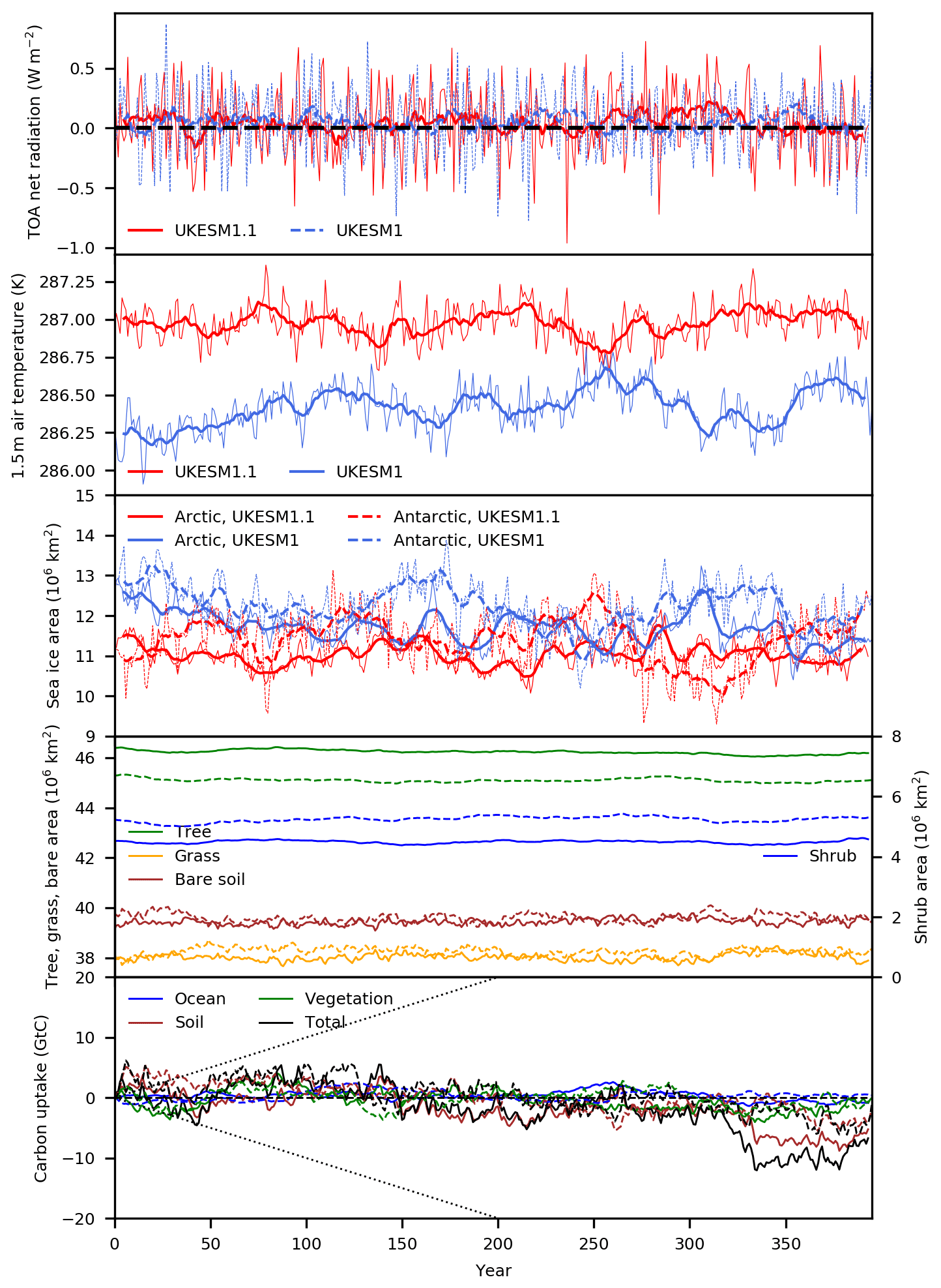
Figure 1Time series of preindustrial climate properties from UKESM1 and UKESM1.1. Plotted from top to bottom are the global annual mean net TOA radiation, global annual mean 1.5 m air temperature, annual mean Arctic and Antarctic sea ice area, global total area of aggregated plant functional types (solid lines for UKESM1.1; dashed lines for UKESM1) and cumulative carbon uptake (solid lines for UKESM1.1, dashed lines for UKESM1 and the dashed black line depicts acceptable drift, following Jones et al., 2016). In the top three panels, UKESM1.1 is plotted in red, and UKESM1 is plotted in blue. An 11-year running mean is plotted with the thicker lines.
4.1 Preindustrial climate stability
The temporal stability of the UKESM1.1 piControl is shown in Fig. 1, which compares the time series of a number of key properties of the preindustrial climate in UKESM1.1 and UKESM1. The net global mean TOA radiation is comparable between the models, with both having a mean net TOA radiation over the 400-year period of approximately 0.04 W m−2 with negligible drift. Both models also show very similar interannual variability.
A key difference in the PI states is the warmer climate of UKESM1.1, which, in the global mean, is up to 0.75 K warmer at the surface than UKESM1. This leads to less sea ice in both the Arctic and Antarctic, with the Arctic showing a larger reduction, and with the annual mean area reducing from about 12.5 million km2 to 11 million km2. Vegetation fractions are also very stable, with negligible changes in grass and bare soil fractions between UKESM1 and UKESM1.1. There is an increase in the tree fraction at the expense of shrubs. This occurs predominantly in the Northern Hemisphere high latitudes and is consistent with a warmer climate, thus enabling a slight northward extension of the boreal treeline.
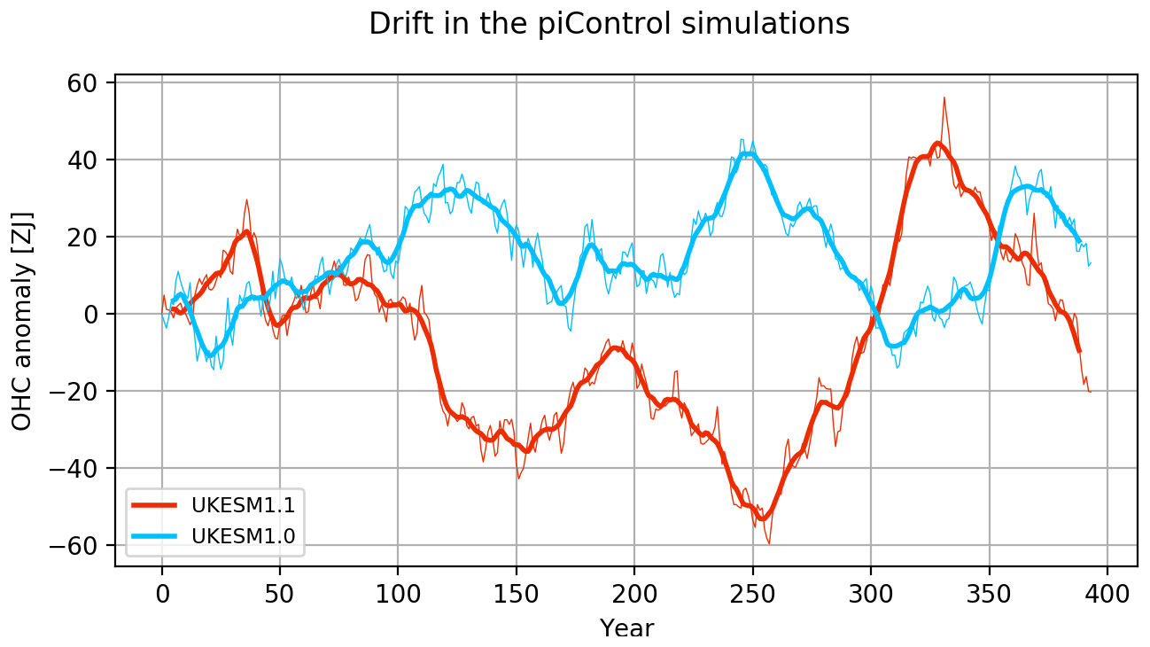
Figure 2Time series of preindustrial ocean heat content anomalies from UKESM1 (red) and UKESM1.1 (blue). Anomalies are calculated relative to the first year of the piControl simulations and an 11-year running mean, which is plotted as in Fig. 1.
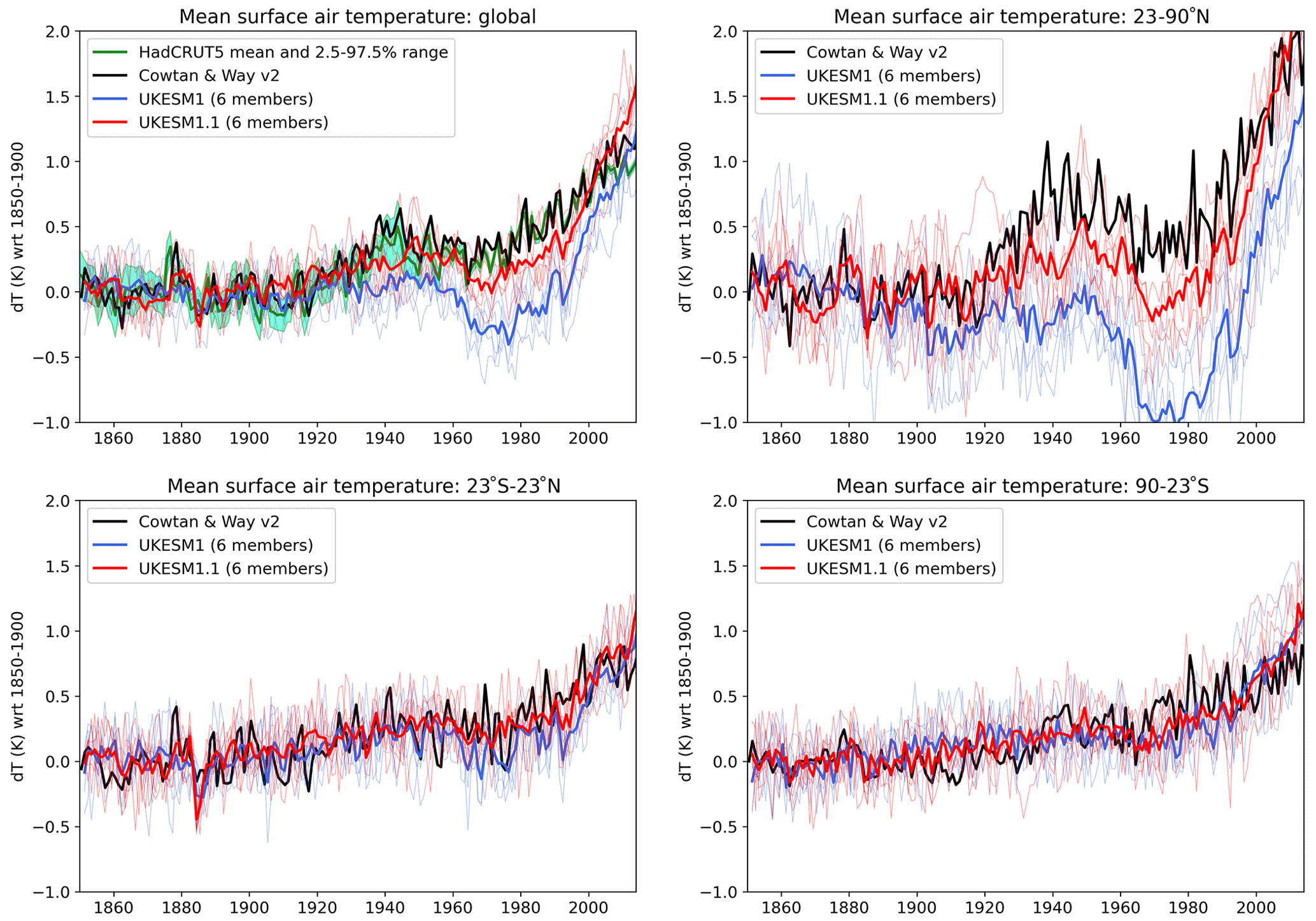
Figure 3Annual mean surface temperature anomaly relative to 1850–1900 mean for the full globe, Northern Hemisphere extratropics (23–90∘ N), tropics (23∘ S–23∘ N) and Southern Hemisphere extratropics (90–23∘ S). Thin lines are the individual historical ensemble members of UKESM1.1 (red) and UKESM1 (blue); the thick line is their ensemble mean. The Cowtan and Way (2014) temperature reconstructions are plotted in black, and for the full globe, the HadCRUT.5.0.1.0 mean and 2.5 %–97.5 % uncertainty range (Morice et al., 2021) are shown in dark green and aquamarine. Model time series are detrended using the linear trend of the preindustrial control over the equivalent period.
Any drift in carbon uptake is well within the allowable threshold of ±0.1 Gt[C] yr−1, which was a requirement for participation in the Coupled Climate–Carbon Cycle Model Intercomparison Project (C4MIP; Jones et al., 2016). The UKESM1 piControl plotted in Fig. 1 is from a much later period than that used in Sellar et al. (2019), and therefore, the drift is noticeably smaller here (see their Fig. 3). The ocean carbon uptake in UKESM1.1 appears to oscillate around zero, while there appears to be more variability in the soil carbon. In particular, after 300 years, there is a sudden increase in the release of soil carbon to the atmosphere.
The variability in global ocean heat content (OHC) in both preindustrial simulations (Fig. 2) shows significant multidecadal variability, whereas the trends are very small (of the order of 1 ZJ per century). As part of this inherent variability, in UKESM1.1 there is a phase of increase in OHC (heat gain for the ocean) from year 250 to year 330. There is a concomitant decrease in Southern Ocean sea ice cover (middle panel in Fig. 1), suggesting a temporary warm spell in the Southern Ocean, together with changes in the regional deepwater formation processes. Sellar et al. (2019), in their Fig. 3, show a comparable centennial variability in a different part of the UKESM1 preindustrial control simulation.
4.2 Evolution of historical climate
4.2.1 Surface temperature
Figure 3 shows the time series of global mean historical surface air temperature anomalies of UKESM1 and UKESM1.1, along with observations from the HadCRUT5 (Morice et al., 2021) and Cowtan and Way (2014) observational datasets. The surface temperature anomalies are calculated relative to the 1850–1900 mean, and even though the drift in the piControl is negligible (see Sect. 4.1), the historical time series is nonetheless detrended using the linear trend of the piControl over the equivalent PI period.
The observations (Fig. 3a) depict a global warming of approximately 0.5 K during the period 1900 to 1940, before cooling slightly in the years following the Second World War and then warming again from the mid-1970s onwards. UKESM1 shows limited warming between 1900 and 1940, followed by excessive cooling beginning in the late 1950s. The model warms during the 1970 to 2014 period, but the rate of warming is overly strong.
The global mean temperature anomaly is generally more positive in UKESM1.1 than UKESM1 throughout the historical period. The two models start to diverge from about 1920, a period coincident with notable increases in anthropogenic SO2 emissions (see Fig. S3). While still underestimating the strength of the warming during the early part of the century, a significant improvement is seen in the anomaly bias against both sets of observations. In particular, the large cold bias from 1960 to the late 1980s is significantly improved in UKESM1.1, with the ensemble mean bias having improved by over 50 %. Both models cool strongly in response to the Mount Pinatubo volcanic eruption in 1991, after which they both tend to warm at the same rate, and UKESM1.1 is slightly too warm by the end of the historical period.
Figure 3 also plots the surface temperature anomalies for the extratropical Northern (NHex) and Southern hemispheres (SHex) and for the tropics. It is evident that the discrepancies between the model and observations are predominantly occurring in the NHex, which lends support to the likely leading role of anthropogenic aerosols in this bias. In general, the individual ensemble members of both models overlap in the observations in both the tropics and SHex. In the SHex, the UKESM1.1 ensemble mean is marginally colder than that for UKESM1, although there is large variability across the ensemble members in this region. While both the tropics and SHex depict a certain amount of interannual variability, they both show a general warming trend during the historical period. In contrast, the different global warming and cooling periods discussed above are clearly originating in the NHex region, pointing to an anthropogenically forced influence. The main impact of UKESM1.1 on the surface temperature is also found to occur predominantly in the NHex. This is where the SO2 deposition changes are expected to have maximum effect due to the majority of anthropogenic SO2 being emitted in this region. The model now captures a slight warming during the 1920 to 1940 period, although still underestimating the magnitude of the warming seen in the observations. The magnitude of the cold bias in the NHex in UKESM1 approaches 1 K at around 1970, while, in UKESM1.1, it is reduced to 0.2–0.3 K.
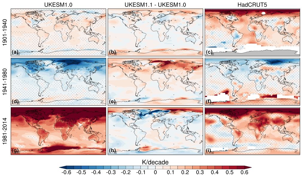
Figure 4Surface temperature trends in (a, d, g) UKESM1 and (c, f, i) HadCRUT5 (Morice et al., 2021) and (b, e, h) the UKESM1.1-UKESM1 difference for the periods (a–c) 1901–1940, (d–f) 1941–1980 and (g–i) 1981–2014. Regions where trends are not significant are stippled.
Figure 4 shows the spatial surface temperature trends in UKESM1 and the difference in trends between UKESM1 and UKESM1.1 for the three distinct anomaly periods (i.e. period of warming (1901–1940), cooling (1941–1980) and warming (1981–2014)) already highlighted above. The surface temperature trends are compared to HadCRUT5 observations (Morice et al., 2021). Between 1901 and 1940, the strongest warming trends are observed in the Arctic, which warms in excess of 0.6 K per decade during this period. Warming trends in excess of 0.2 K per decade are also observed over most ocean basins and Northern Hemisphere continents. Changes in surface temperature trends in UKESM1.1 relative to UKESM1 are small during this period, and the models generally underestimate the magnitude of the warming trends globally. The models also fail to capture the localised regions of continental cooling. The largest change in the surface temperature trend between UKESM1.1 and UKESM1 is found between 1941 and 1980. The trends are more positive in UKESM1.1 during this period, with the largest changes occurring across the Northern Hemisphere (NH) high-latitude regions, where the model trends are warmer by up to 0.4 K per decade. This significantly improves the negative bias in the temperature trends during this period. Warming trends observed over central Asia and in the Southern Hemisphere (SH) high latitudes are not captured well in the models, although these trends appear not to be statistically significant. The sign of the temperature trends changes from a predominantly cooling trend in the 1941–1980 period to a predominantly warming trend between 1981 and 2014. This change coincides with the time period in which globally averaged anthropogenic SO2 emissions peak before stabilising and subsequently declining, following the implementation of clean air legislation (see Fig. S3). During the 1981–2014 period, both models warm too fast everywhere, but this strong warming trend is generally reduced in UKESM1.1. This improves agreement with the observations, particularly in the NH, although the more positive trends in the Arctic region further degrade the model bias here. Failure to capture the observed cooling trend over the Pacific Ocean is another common feature across CMIP6 models (Dittus et al., 2021). Several causes for this possible bias have been proposed, including errors in the internal variability, biased responses to volcanic eruptions or the circulation response to anthropogenic aerosols, among others. The weaker warming trends off the western coasts of North and South America improve the model bias in these regions, but biases persist in the tropical Pacific.
4.2.2 Aerosols and clouds
The main science updates included in UKESM1.1 alter the distribution and evolution of aerosols and their interactions within the full ESM. In order to investigate the possible drivers of the improved historical surface temperature record presented above, here we examine the change in the historical evolution of key aerosol and cloud properties and how this alters the SW radiative fluxes.
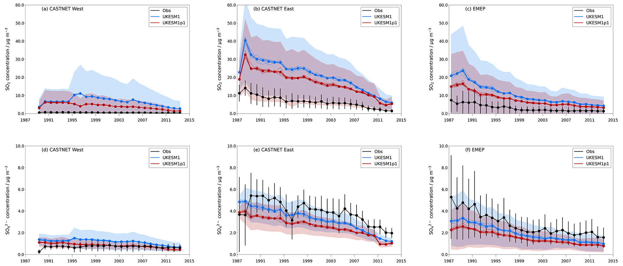
Figure 5Comparison of annual mean (a–c) surface SO2 concentration and (d–f) surface SO4 aerosol concentration across a network of North American (Clean Air Status and Trends Network – CASTNET) and European (European Monitoring and Evaluation Programme – EMEP) measurement sites. CASTNET stations have been grouped into eastern and western sites as determined by their location east and west of 100∘ W.
Hardacre et al. (2021) conduct an in-depth evaluation of the impact of the updated SO2 dry deposition parameterisation on the surface SO2 and SO4 concentrations in UKESM1 using both ground-based and satellite data. The simulations assessed in that study also include the updates to the DMS chemical reactions (see Table 1) and the bug fix for the updating of H2SO4 concentrations but do not include any of the other changes implemented in UKESM1.1. The increase in SO2 dry deposition in UKESM1.1 reduces the global SO2 gas and SO4 aerosol burdens. Figure 5 compares the surface SO2 and SO4 concentrations with surface measurements across Europe and North America. Full details of the observational data are provided in Hardacre et al. (2021). Similar to the findings in Hardacre et al. (2021), a notable improvement in the positive surface SO2 concentration bias is found in UKESM1.1. A corresponding reduction in SO4 aerosol concentrations degrades the pre-existing negative bias (Mulcahy et al., 2020; Hardacre et al., 2021). This points to the possibility of further compensating biases in the sulfur cycle, with too little SO2 loss via chemical oxidation of SO2 by OH and O3 combined with potentially too large anthropogenic emissions of SO2 being compensated for here by dry deposition.

Figure 6Historical evolution of anomalies in aerosol optical depth (550 nm), cloud droplet number concentration and cloud effective radius across the Northern Hemisphere extratropics in UKESM1 (blue) and UKESM1.1 (red). Both cloud droplet number concentration and effective radius represent cloud-top values, and anomalies are calculated relative to the 1850–1900 mean. Both the ensemble mean (thick lines) and individual ensemble members (fainter lines) are plotted. A 5-year running mean has been applied to the annual mean model output.
Simulated anomalies of the annual mean AOD, cloud droplet number concentration (Nd) at cloud-top and cloud droplet effective radius (reff) at cloud-top over the historical period are presented for the NHex region in Fig. 6 (the historical evolution of the global annual mean absolute values is shown in Fig. S12). The anomalies are calculated relative to an 1850–1900 mean. Both the AOD and Nd begin to steadily increase early in the 20th century, with a more rapid increase occurring from about 1950 for both variables. The increase in Nd is accompanied by a corresponding decrease in the reff. Anomalies in all three variables peak around 1980 before slowly declining.
Clearly the evolution of the aerosol and cloud properties is closely tied to the evolution of the anthropogenic SO2 emissions (Fig. S3). While both models show a similar temporal evolution in AOD, Nd and reff, the anomalies in UKESM1.1, are systematically smaller in all cases. The strong increasing trend in AOD and Nd over the 1940 to 1990 period simulated by UKESM1 is weaker in UKESM1.1, with peak anomaly values reduced by approximately 30 % in both variables and the anomaly in reff reduced by approximately 10 %.
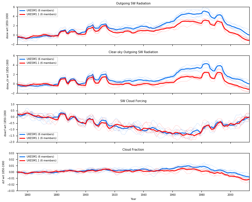
Figure 7Historical evolution of anomalies in all-sky and clear-sky outgoing SW radiation, SW cloud forcing and cloud fraction relative to the 1850–1900 mean in UKESM1 (blue) and UKESM1.1 (red). Both the ensemble mean (thick lines) and individual ensemble members (fainter lines) are plotted. A 5-year running mean has been applied to the annual mean model output.
The smaller anomalies in AOD and Nd in UKESM1.1 relative to UKESM1 contribute to reductions in the TOA outgoing shortwave (OSW) radiation (Fig. 7). The anomaly in OSW over the historical period has some large interannual variations associated with the large volcanic eruptions. Overall, however, there is a general increasing trend in OSW throughout the 20th century, peaking again in 1980. The positive anomalies in both clear-sky and all-sky OSW are smaller throughout the period in UKESM1.1 by between 30 % and 40 %. The difference in the SW cloud forcing anomaly is negligible between the two models, suggesting that the reduced anomaly in the clear-sky OSW radiation is a key driver of the warmer surface temperature anomalies in UKESM1.1. However, the absolute SW cloud forcing is notably less negative in UKESM1.1 compared to UKESM (see Fig. S13), which will also contribute to a more positive net TOA radiation balance and, subsequently, warmer surface temperatures in UKESM1.1.
The lack of historical observations of aerosol and cloud properties precludes an evaluation of the evolution of these properties and their trends over the full historical period. We are therefore reliant on observations of the more recent past to give us an indication of the skill of the models in simulating these properties in the present day. Such an evaluation will provide useful evidence as to the overall skill of the aerosol simulation in the updated UKESM1.1 configuration.
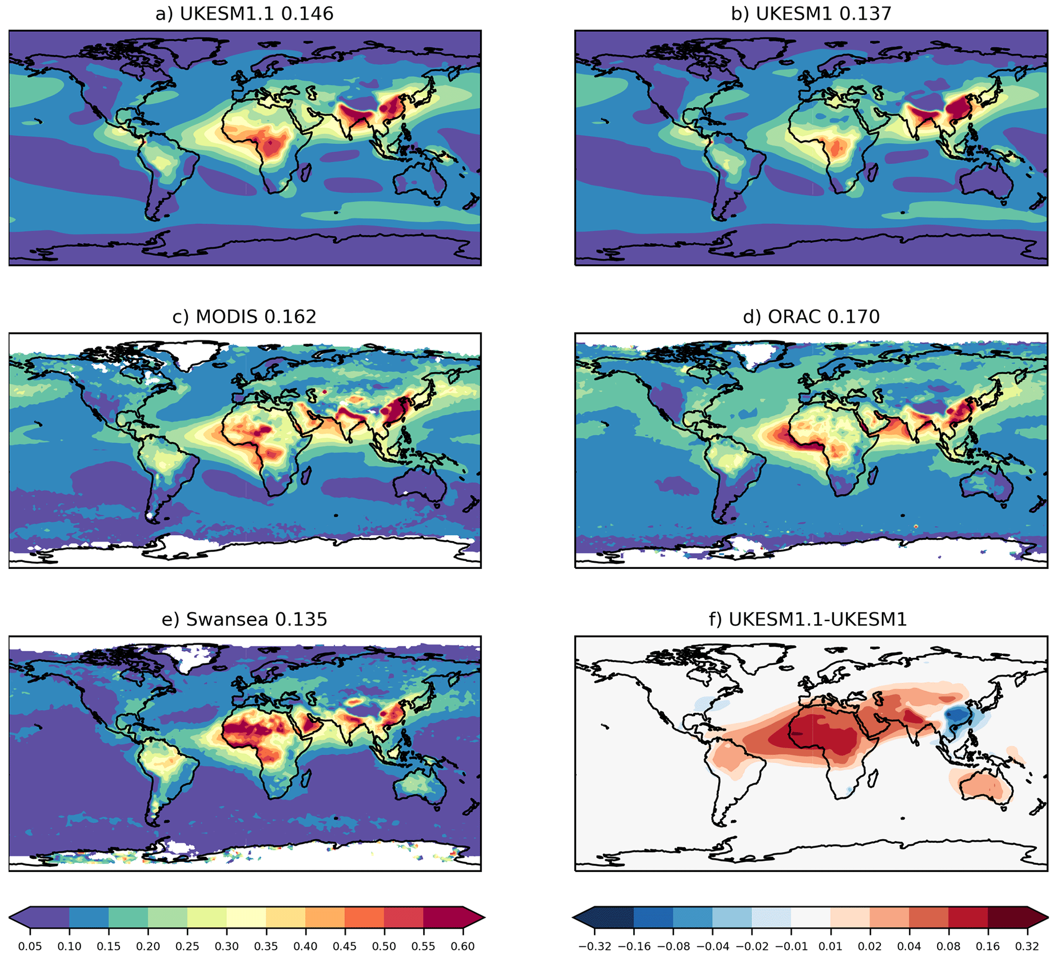
Figure 8Annual mean AOD at 550 nm from (a) UKESM1.1. (b) UKESM1 simulations over the 2003–2014 period. Satellite-derived AOD over the same period from (c) MODIS c6 (Hsu et al., 2004), (d) ORAC (Optimal Retrieval of Aerosol and Cloud; Thomas et al., 2009) and (e) Swansea retrieval algorithms (Bevan et al., 2012). (f) UKESM1.1 − UKESM1 AOD difference. The global mean AOD from models and satellites are shown in the panel title.
Annual mean AOD over the 2003 to 2014 period is compared to a number of satellite AOD products in Fig. 8. These products, their uncertainties and details of the evaluation procedure are described in detail in Mulcahy et al. (2020). The time period is chosen to match the available satellite data record. Despite a reduction in the positive anomaly in AOD over the historical period (Fig. 6), the global mean AOD in UKESM1.1 is higher than UKESM1 by about 7 %. This is due to the revised dust tuning in UKESM1.1, which increases the dust AOD over and downwind of the major dust source regions. The higher AOD improves low model biases in these regions; in particular, the low bias over the Sahara desert, tropical Atlantic and the Arabian Sea are in better agreement with the satellite data. Increased AOD over Australia improves the agreement with the ORAC and Swansea products but introduces a positive bias against MODIS. Reductions in AOD can be seen in the important anthropogenic emission source regions of China and northeastern America, with the reductions in China being the largest due to the much higher SO2 emissions in China during this period. Interestingly, reductions in AOD over Europe are not found. Emissions of SO2 in Europe are much reduced by 2003, and so contributions of SO4 to the total AOD will be relatively smaller during this time. Furthermore, any decrease in AOD due to changes in SO4 load has potentially been offset by a corresponding increase in AOD from dust transported from the Sahara. The reduction in AOD over China improves the large positive bias in this region, and the spatial heterogeneity in the observed AOD over this region is better captured in UKESM1.1. While the uncertainty in the satellite products can be large, UKESM1 AOD was on the lower end of the satellite AOD range (Mulcahy et al., 2020), and UKESM1.1 now comfortably sits in the middle of this range.
The ground-based AERONET network of AOD measurements (Holben et al., 1998) provides another source of reliable AOD measurements with lower uncertainties than the satellite products (Holben et al., 2001). A comparison of the simulated AOD at 440 nm, with a long-term climatology of measurements from 67 AERONET sites, is shown in Fig. S4. Both the root mean square error and correlation coefficient are improved in UKESM1.1. Agreement is generally improved at measurement sites in the Sahel, Saudi Arabia and the Caribbean. The AOD gradient from western to eastern USA also appears to be better captured.
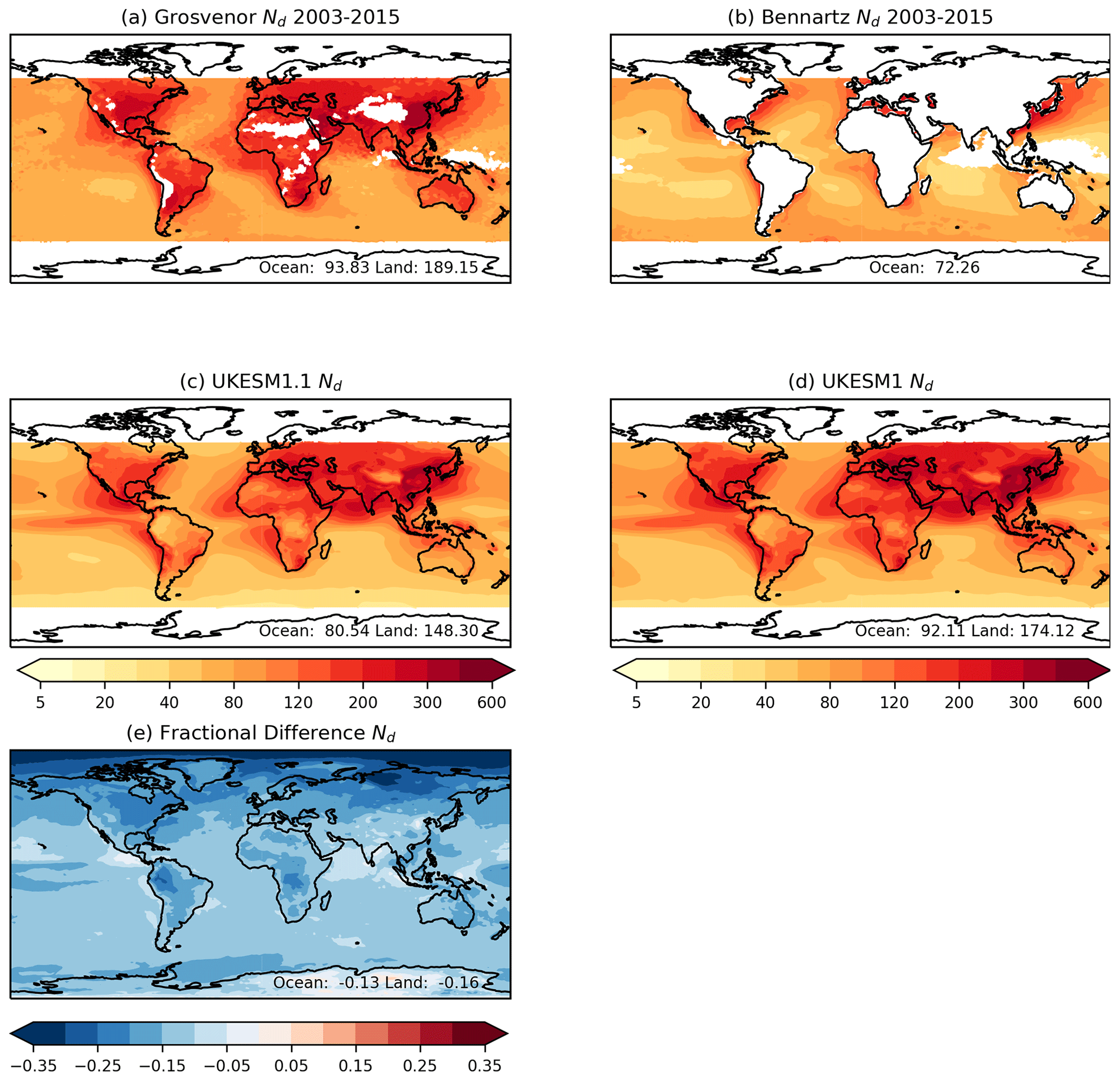
Figure 9Observed and simulated annual mean cloud droplet number concentration at the cloud-top Nd (cm−3), from (a) Grosvenor et al. (2018), (b) Bennartz and Rausch (2017) satellite products and simulated Nd from (c) UKESM1.1 and (d) UKESM1. (e) UKESM1.1 − UKESM1 Nd fractional difference. The mean ocean and land Nd values are displayed in the subpanels.
In UKESM, mineral dust is treated as hydrophobic and therefore cannot act as cloud condensation nuclei. The global mean increase in AOD is therefore not translated into a corresponding increase in cloud droplet number concentration, which will respond more to the changes in SO4 aerosol in this configuration. There is a global-scale reduction in present-day cloud-top Nd in UKESM1.1 (Fig. 9), with reductions being marginally higher over land (reduced by 16 %) than ocean (reduced by 13 %) surfaces. Reductions in Nd are much higher in the NH, with reductions of approximately 30 % in the NH high latitudes. Again, there is large uncertainty in the satellite retrievals of Nd, as discussed in Mulcahy et al. (2020), and the spatial distribution and magnitude of Nd in both model configurations lies within this observational uncertainty. While UKESM1 arguably is closer to the Grosvenor et al. (2018) product, UKESM1.1 now sits within the two satellite estimates.
4.2.3 Ocean heat content
Changes in ocean heat content (OHC) account for 91 % of the increase in the global energy inventory (Forster et al., 2021). Changes in ocean heat content are therefore a more reliable indicator of Earth's energy imbalance than, for example, sea surface temperature (von Schuckmann et al., 2016). Here we assess the capability of UKESM1.1, compared against UKESM1, to reproduce the observed increase in OHC during the historical period.
There are various observation-based datasets of historical OHC. Most of them are based on the same in situ observations of ocean temperature but use different methods for infilling gaps in observations and for correcting instrumental biases (Boyer et al., 2016). The coverage of in situ observations is sparse below a depth of 2000 m and before 1960 in the upper layers. We use a selection of OHC observational datasets to illustrate this observational range, i.e. NCEI (Levitus et al., 2012), C2020 (Cheng et al., 2020), EN421 (Good et al., 2013), DOM+LEV (Domingues et al., 2008; Levitus et al., 2012), ISH (Ishii et al., 2017) and CHG (Cheng et al., 2017). For depths below 2000 m, we used the OHC trend estimate from Purkey and Johnson (2010). The historical simulations are detrended by diagnosing the linear trend from the matching part of the piControl and subtracting it from the historical simulation. OHC anomalies are calculated relative to a 2005–2014 mean, as this period is best covered by the observations and enables a more realistic model–observation comparison.
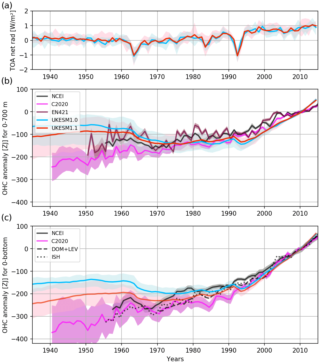
Figure 10(a) TOA net radiation, (b) 0–700 m global ocean heat content (OHC) anomaly and (c) full-depth global OHC anomaly for the UKESM1.1 (red) and UKESM1 (blue) historical simulations. Observation-based OHC time series (b, c) are plotted in black, purple and maroon. TOA net radiation time series are anomalies with respect to the average of 1850–1870. OHC time series (simulations and observations) are anomalies with respect to the average of 2005–2014. Shading shows the range of the ensemble for simulations and the standard error for the observational data.
In the 0–700 m ocean layer (Fig. 10b), the simulations are reasonably close to observations from about 1960 onwards. Prior to 1960, the observations indicate a larger change in OHC than is simulated by the UKESM ensembles. While UKESM1.1 is notably closer to observations than UKESM1, both model versions indicate little change in OHC during the 1970s and 1980s and do not capture the observed increase of 50 ZJ. After 1991, the rate of OHC change in both model versions is stronger than observed. This is partly a consequence of the high climate sensitivity of these models (see Sect. 4.3) responding to the increase in greenhouse gas concentrations in this period. The models appear to react strongly to the 20th century volcano eruptions in 1963 (Agung), 1982 (El Chichón) and 1991 (Pinatubo; see Fig. 10a), with a marked loss in OHC of the order of 10 or 20 ZJ (Fig. 10b). In particular for the Pinatubo eruption in 1991, observations do not seem to indicate such a loss of global OHC (Gregory et al., 2020). The UKESM processes responsible for this strong reaction are currently under investigation.
For the entire global ocean (Fig. 10c), the model performance is different to that of the 0–700 m layer. The performance improvement in UKESM1.1 is much larger for the entire global ocean. The total 1950–2014 OHC increase is about 40 % larger in UKESM1.1, bringing it much closer to observations. For the period since 1991 the rate of OHC change is still larger than observations but only marginally so. This implies that, in the ocean layers below 700 m, the uptake of heat is too small during this period, compensating for the overly strong increase above 700 m.
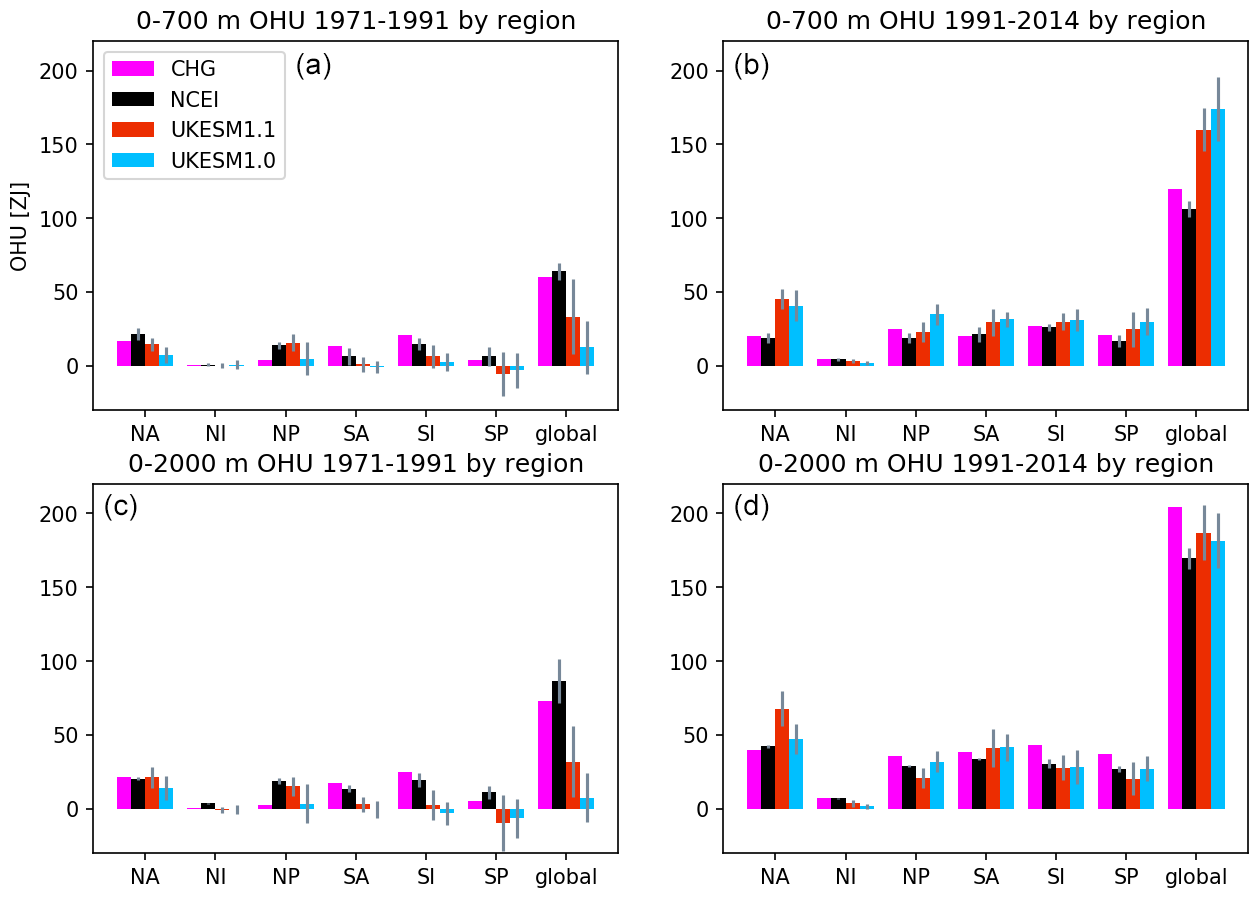
Figure 11Ocean heat uptake (OHU) for six ocean basins and the global ocean in the 0–700 m layer (a, b) and the 0–2000 m layer (c, d) for the 1971–1991 period (a, c) and the 1991–2014 period (b, d). Colour code as in Fig. 10. Thin grey bars give the standard error in the observational datasets and the ensemble standard deviation for the model ensembles. The ocean basins included are the North and South Atlantic (NA and SA) oceans, North and South Indian (NI and SI) oceans, North and South Pacific (NP and SP) oceans.
A regional breakdown of OHC changes since 1971 is given in Fig. 11. The ocean basins employed are the Atlantic, the Indian and the Pacific, each separated at the Equator into a Northern and a Southern hemisphere section. We analyse ocean heat uptake (OHU; defined as the change in OHC) for two consecutive periods. The period 1971–1991 represents a period of small ocean heat uptake, while in the period 1991–2014 the OHU is much larger. We used the 0–2000 m layer here instead of the full-depth ocean because no OHC trend estimates for individual basins are available below 2000 m. For 1971–1991 (Fig. 11), we see a clear improvement in UKESM1.1, on average capturing about half of the observed OHU (in 0–700 m). This increase comes mainly from the North Atlantic (NA) and North Pacific (NP) basins, thus responding to the less negative anthropogenic aerosol ERF in UKESM1.1 (see Sect. 4.3). In contrast to observations, we see negative OHU (loss of heat from the ocean) in the South Indian (SI) and South Pacific (SP) basins. We suggest that this is heat loss from simulated open-ocean deepwater formation (Menary et al., 2018), which does not correctly capture the actual deepwater formation processes on the Antarctic shelves.
In the 1991–2014 period, we see again that both model versions simulate too much OHU in the 0–700 m layer. The source of this excess heat is mainly the North Atlantic and, to some extent, the South Atlantic as well. Kuhlbrodt et al. (2018, see their Fig. 8) showed a similar strong warming trend in the deep Atlantic in HadGEM3-GC3.1-LL, the physical core model of UKESM1 and UKESM1.1. It is possible that this tendency for strong deep Atlantic OHU is the underlying reason here.
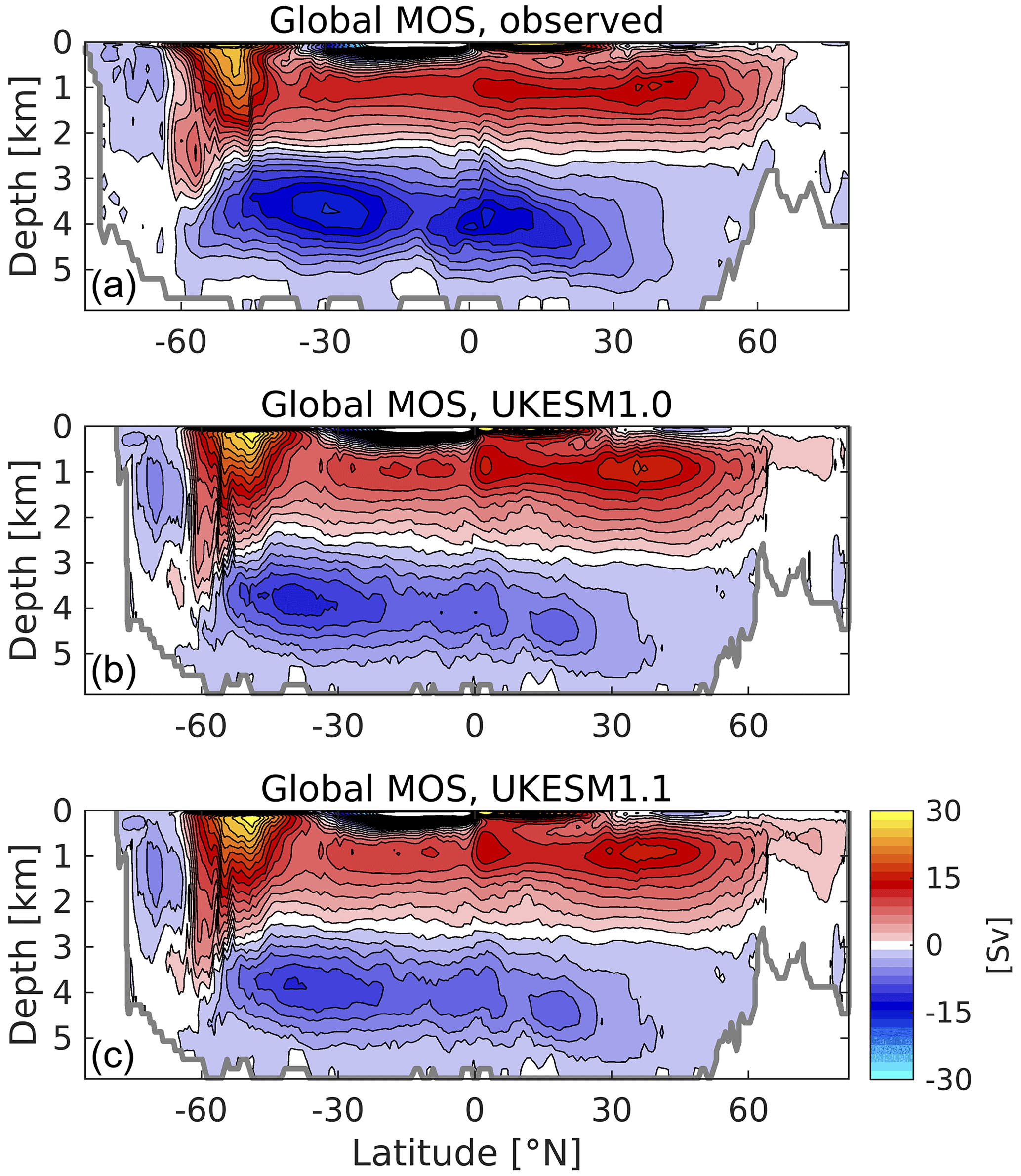
Figure 12Observationally derived (a) and UKESM1 (b) and UKESM1.1 (c) meridional overturning circulation (MOC) for the global ocean. The observational circulation is derived from the Estimating the Circulation and Climate of the Ocean (ECCO) V4r4 circulation reanalysis for the period 1992–2017. The model circulation shown is based on the decadal mean streamfunction for the period 2000–2009, averaged across the members of both model ensembles. Both plots include the components from parameterised mesoscaled eddies (Gent and McWilliams, 1990; Gent et al., 1995). MOC is in sieverts with a contour interval of 2 Sv.
4.2.4 Ocean circulation
Yool et al. (2021) highlight a number of biases in the interior ocean circulation in UKESM1, such as insufficient vertical mixing leading to surface heat biases and dampened deepwater circulations. Here we examine the impact of the different atmospheric forcing in UKESM1.1, driven primarily by weaker anthropogenic aerosol forcing, on these biases. Figure 12 shows the global streamfunction of the ocean's meridional overturning circulation (MOC), produced by the Estimating the Circulation and Climate of the Ocean consortium (ECCO; Forget et al., 2015; Fukumori et al., 2021) ocean reanalysis, and compares it with UKESM1 and UKESM1.1. Both model MOCs are broadly consistent with the ECCO reanalysis. Both exhibit a stronger maximum MOC at 40∘ N, and a slightly weaker Antarctic Bottom Water (AABW) cell northward of 60∘ S. The maximum strength of the AABW cell in UKESM1.1 is at 45∘ S and is slightly weaker than that of UKESM1, but otherwise, the models perform very similarly.
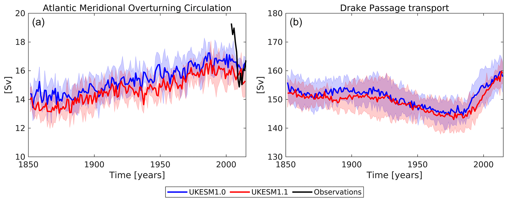
Figure 13Atlantic meridional overturning circulation (AMOC; a) and Drake Passage transport (b) for the UKESM1 (blue) and UKESM1.1 (red) ensembles. Solid lines denote the ensemble mean, with shaded areas marking ±1 standard deviation. Estimated AMOC transport derived from the RAPID array (Smeed et al., 2018) is shown in black for the period of available observations.
On a regional scale, Fig. 13 shows the complete historical time series for the Atlantic meridional overturning circulation (AMOC) and Drake Passage transport. The observational mean for the AMOC for the period 2004–2014 is 16.8 Sv (Smeed et al., 2018), compared with simulated magnitudes of 16.4 and 15.7 Sv for UKESM1 and UKESM1.1 respectively. Driven by anthropogenic aerosol-mediated cooling of the Northern Hemisphere (Menary et al., 2013, 2020; Robson et al., 2020), the AMOC strength exhibits a ramping-up throughout the 20th century, followed by a decline into the 21st century. The slightly lower AMOC in the UKESM1.1 ensemble mean is consistent with a less negative aerosol forcing in the UKESM1.1 simulations, although there is considerable variability across the ensemble members, leading to the configurations largely overlapping, particularly in the first half of the simulated period (1850 to approximately 1940). The Drake Passage transport is estimated at 173 Sv (Donohue et al., 2016), with simulated magnitudes of 157.5 and 156.7 Sv for UKESM1 and UKESM1.1 respectively (for the period 2004–2014). UKESM1.1 shows very similar magnitudes to UKESM1 for both major transports, if slightly lower on average for both. The temporal patterns of both transports across the historical period are also very similar.
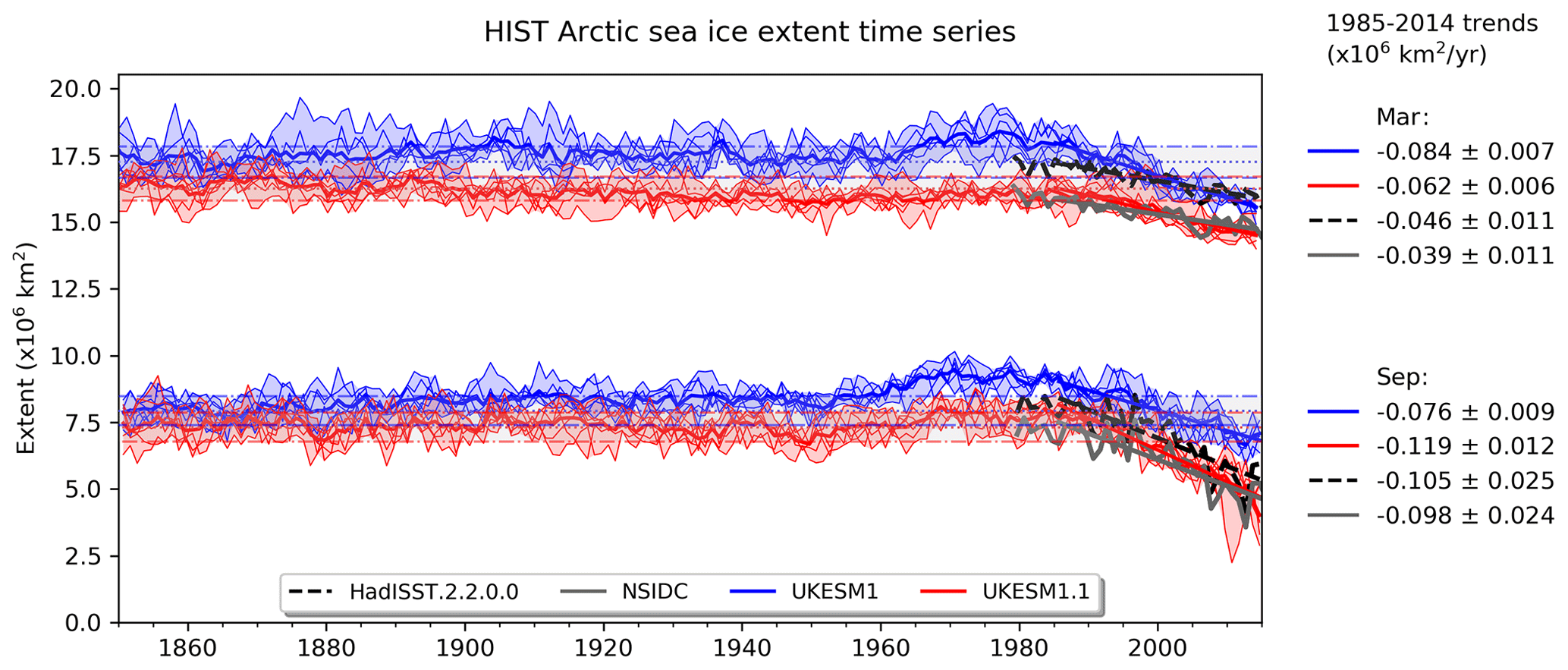
Figure 14Time series of simulated (blue, UKESM1; red, UKESM1.1) and observed (black, HadISST; grey, NSIDC) sea ice extent in the Arctic for the months of March and September over the full historical period (1850–2014). The seasonal trends in the more recent period are shown for each dataset on the right-hand side. Model data represent the ensemble mean for UKESM1 (six members) and UKESM1.1 (six members), with the ±1 standard deviation also shown.
4.2.5 Sea ice
The cold bias in UKESM1 drives positive biases in Arctic sea ice extent and thickness (Sellar et al., 2019; Yool et al., 2021). Here we examine what impact the warmer climate in UKESM1.1 has on sea ice properties in both the Arctic and Antarctic. Previous studies have highlighted a strong negative correlation between global mean surface temperature and Arctic sea ice extent (Rosenblum and Eisenman, 2017; Mahlstein and Knutti, 2012). Figure 14 shows the historical time series of sea ice extent in the Arctic for the months corresponding to periods of maximum (March) and minimum (September) sea ice in this region. In both seasons, the warmer climate in UKESM1.1 leads to a reduction in sea ice extent and volume throughout the historical period. Observational estimates from the HadISST (HadISST.2.2.0.0; Titchner and Rayner, 2014) and NSIDC (National Snow and Ice Data Center; Fetterer et al., 2017) datasets available from 1979 onwards are also plotted. While UKESM1 agrees better with sea ice extent of the HadISST data in March, it is positively biased against NSIDC. UKESM1.1 therefore moves further away from the HadISST data but agrees well with NSIDC. In September, the observational data are in better agreement with each other and with UKESM1.1, while UKESM1 is positively biased against both. The trend in observed Arctic sea ice extent (and volume) is negative over the observed period, with a stronger negative trend evident during sea ice minimum periods. Both models also simulate decreasing trends during this period. However, in UKESM1, the trend is too strong in March, indicating that the model simulates a faster rate of loss of sea ice in this region than observed. Meanwhile, the very high ice thickness in the central Arctic means that the UKESM1 trend in September is too weak. In UKESM1.1 the trends are in better agreement with the observed trends during both periods.
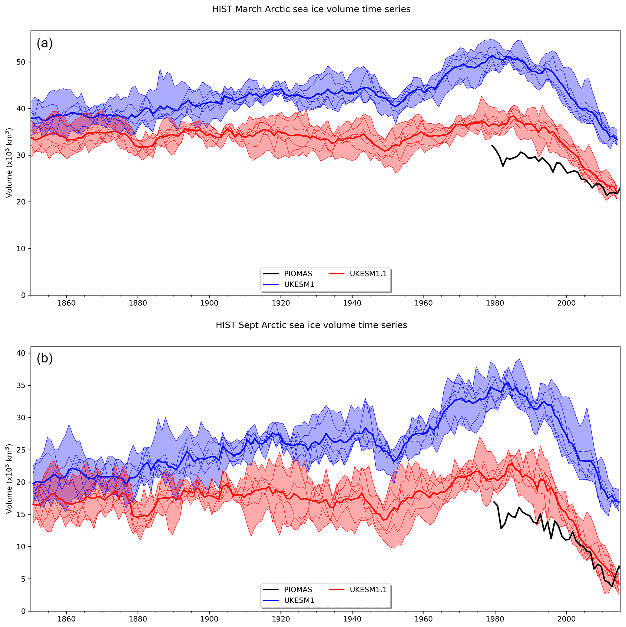
Figure 15Time series of simulated (blue, UKESM1; red, UKESM1.1) sea ice volume in the Arctic for the months of (a) March and (b) September over the full historical period (1850–2014) along with the Pan-Arctic Ice Ocean Modeling and Assimilation System (PIOMAS) reanalysis data (black). Model data represent the ensemble mean for UKESM1 (six members) and UKESM1.1 (six members), with the ±1 standard deviation also shown.
Figure 15 shows the historical time series of the Arctic sea ice volume for the same months. Large positive biases in the Arctic sea ice volume found in UKESM1 are significantly improved in UKESM1.1 in comparison with the commonly used Pan-Arctic Ice Ocean Modeling and Assimilation System reanalysis dataset (PIOMAS; Schweiger et al., 2011). UKESM1 simulates a positive trend in sea ice volume throughout the historical period, with a notable increase occurring around 1950 before reaching peak volume in 1980 and declining steadily to the present day. By contrast, UKESM1.1 shows a minimal trend in the ensemble mean up to 1950, followed by a much smaller increasing trend after this before declining at a similar rate to UKESM1. UKESM1.1 is in better agreement with the PIOMAS dataset during the reanalysis period post-1975, reaching comparable present-day volumes. However both models decrease too sharply after 1980. Consistent with the minimal changes in Southern Hemisphere temperature, there is no significant difference in Antarctic sea ice extent or volume between UKESM1 and UKESM1.1 (see Figs. S5 and S6). Both models simulate a flat trend in both extent and volume up until the late 1970s, after which the extent and volume decrease at similar rates in both models. Observations of sea ice extent from 1979 show a small positive trend which is not captured by the models.
4.2.6 Ocean biogeochemistry
The ocean biogeochemistry model in UKESM1.1 remains unchanged from UKESM1, and changes in the marine biogeochemical properties are therefore small and are solely driven by the changes in the physical climate and coupled interactions such as the iron deposition to the ocean. Figure S7 demonstrates the strong agreement in both the magnitude and temporal pattern of the ocean CO2 uptake over the historical period. The total integrated CO2 uptake over this period differs by less than 0.1 Pg C between UKESM1 and UKESM1.1.
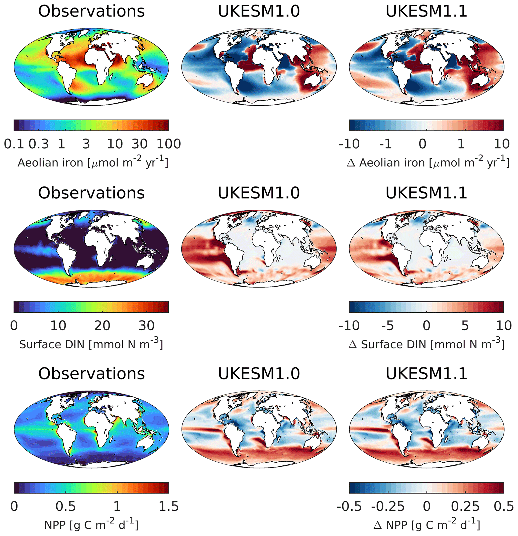
Figure 16Spatial distributions of (left) observed (top) iron deposition to the ocean (middle row), dissolved inorganic nitrogen (DIN) and (bottom) net primary production (NPP), along with simulated biases from (middle column) UKESM1 and (right) UKESM1.1.
The global mean net primary production (NPP) is also very similar in both models across the historical period, although UKESM1.1 (46.6 Pg C yr−1) is consistently lower than UKESM1 (47.9 Pg C yr−1; Fig. S7). Changes in the spatial distribution of NPP are also very small (Fig. 16) and highlight common regional biases such as the positive bias in the Southern Ocean and negative biases in the subequatorial ocean basins. Changes in surface nitrogen nutrient biases relative to the observed climatology of Garcia et al. (2013) are more noticeable, with lower positive biases in the Southern Ocean and, particularly, the equatorial Pacific. In examining UKESM1, Yool et al. (2021) attribute this latter bias in part to more extreme iron stress in this region caused by low biases in dust deposition from the atmosphere. The patterns of this deposition in UKESM1 and UKESM1.1 (Fig. 16) both differ from that of the observational estimate of Mahowald et al. (2005). In particular, fluxes are too small in the equatorial Pacific and Southern oceans in both models. These biases are generally improved in UKESM1.1 due to the shift in atmospheric dust size distribution to smaller particles leading to more transport of dust over the remote oceans and therefore enhanced oceanic deposition. However, increases in dust deposition across the maritime continent and around Australia increase positive biases in these regions. In general, the higher dust deposition to the ocean surface reduces iron stress and simultaneously increases nitrogen uptake and loss from the surface, reducing surface concentration biases (Fig. 16). On balance, this results in the model being slightly more nutrient-stressed at the surface, reducing productivity, but the overall changes in net primary productivity are small and do not noticeably impact the bias.
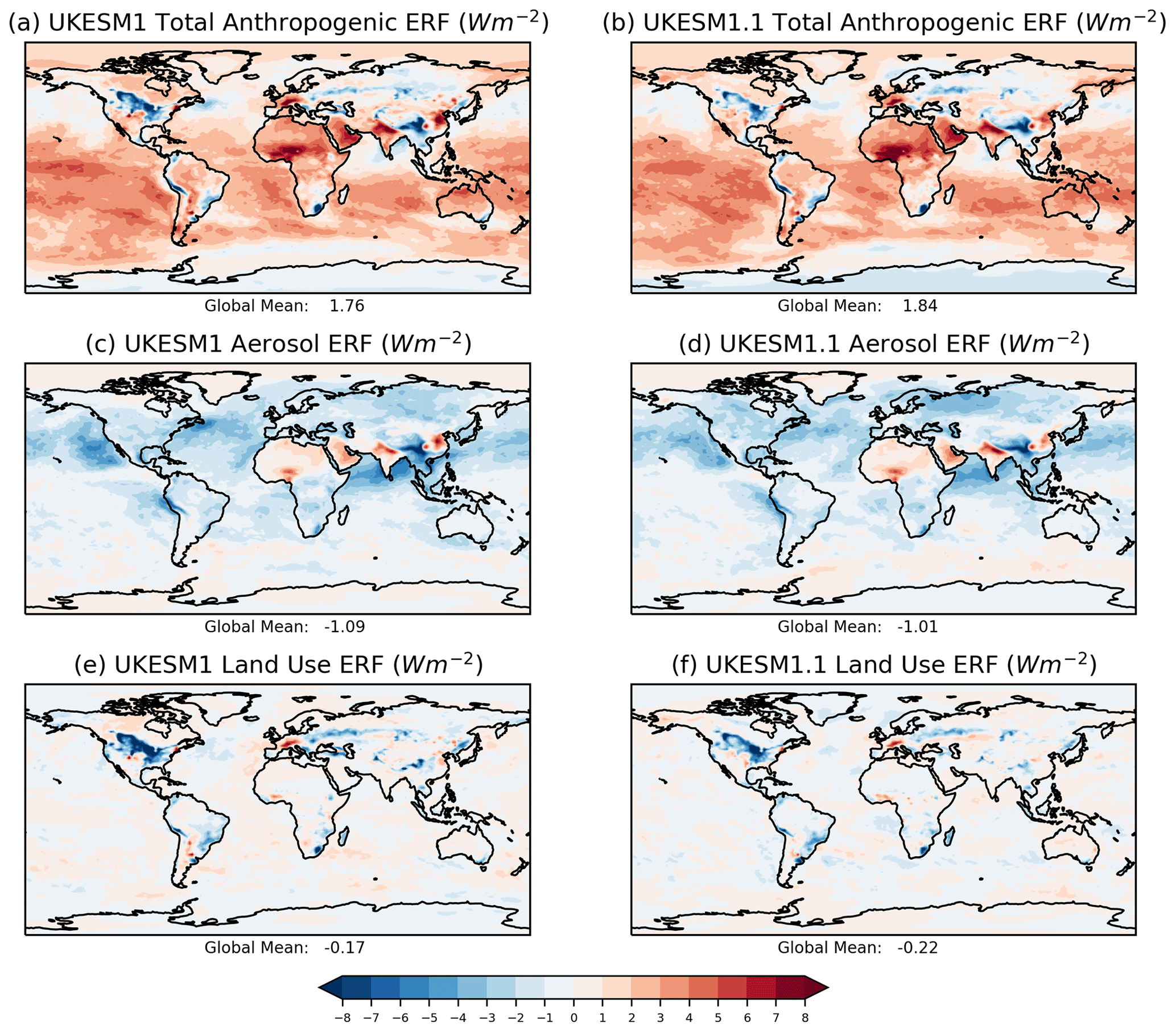
Figure 17Comparison of the anthropogenic effective radiative forcing (ERF) in (a, c, e) UKESM1 and (b, d, f) UKESM1.1. (a, b) The total anthropogenic ERF, (c, d) aerosol ERF and (e, f) land use change ERF. The ERFs are calculated for the year 2014 relative to an 1850 preindustrial control, following Pincus et al. (2016).
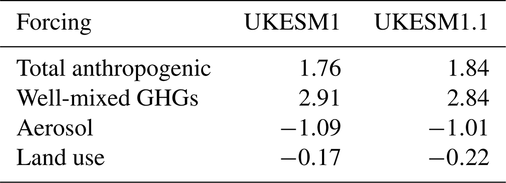
Table 3Global annual mean effective radiative forcings (W m−2) in UKESM1.1 and UKESM1. UKESM1 values are taken from O'Connor et al. (2021). The ERFs are calculated for the year 2014 relative to an 1850 preindustrial control climate (Pincus et al., 2016). Note that GHGs are greenhouse gases.
4.3 Forcing and climate sensitivity
We now compare the key effective radiative forcings between UKESM1.1 and UKESM1 and examine their potential role in the improved simulation of historical surface temperature. Figure 17 compares the all-sky total anthropogenic, aerosol and land use ERF from UKESM1 and UKESM1.1, and the global mean values are summarised in Table 3. The total anthropogenic ERF is more positive in UKESM1.1, increasing from 1.76 to 1.84 W m−2. This is in part due to a less negative aerosol ERF which has increased from −1.09 to −1.01 W m−2. Most of the change in the aerosol ERF comes through changes in the clear-sky forcing, which has increased by 0.2 W m−2 (see Fig. S8). This implies that the aerosol–cloud forcing in UKESM1.1 is more negative than UKESM1 by about 0.1 W m−2. The increases in aerosol ERF are seen predominantly across the NH, although there are also regions of more positive aerosol forcing across the Southern Ocean, possibly due to changes in the background natural loading of SO4 aerosol derived from marine DMS sources.
Table 4The SW components of the aerosol effective radiative forcing (W m−2) in UKESM1.1 and UKESM1.

Using the piClim-control and piClim-aer experiments, we further decompose the aerosol ERF into its SW components using the approximate partial radiative perturbation (APRP) technique (Zelinka et al., 2014; Taylor et al., 2007). Given that aerosols predominantly perturb the SW part of the spectrum, this enables an estimation of the aerosol ERF due to aerosol–radiation interactions (ARIs) and aerosol–cloud interactions (ACIs) separately. The results are summarised in Table 4. The net SW forcing has increased by 0.13 W m−2. This weaker aerosol forcing is almost entirely due to smaller (more positive) clear-sky scattering component which is offset somewhat by a small strengthening in the SW cloud component. The most notable change in the latter appears to come from an increase in the cloud amount contribution. However, the net SW cloud differences due to aerosols are relatively small (−0.045 W m−2) overall.
The SO2 dry deposition changes not only reduce the SO2 and subsequently SO4 aerosol concentrations in the piClim-aer simulation but also change the preindustrial aerosol concentration through reductions in SO4 aerosol derived from natural marine emissions of DMS, thus essentially leading to a cleaner PI atmosphere. In addition, smaller changes to the overall SO4 burden and natural background Nd are expected from the DMS chemical reaction changes, in addition to the bug fix in the aerosol activation (see Sect. 2.1), which leads to lower preindustrial Nd concentrations (reduced by 14 %) in UKESM1.1 and contributes to a notably less negative SW cloud forcing (see also Fig. S13). A cleaner preindustrial climate will strengthen the magnitude of the anthropogenic aerosol effective radiative forcing (ERF) from aerosol–cloud interactions (Carslaw et al., 2013). At the same time, the preindustrial clear-sky AOD is 8 % higher in UKESM1.1 due to the increased dust concentrations, which offsets the global mean AOD reduction due to the reduced sulfate aerosol load. This, combined with the lower anthropogenic SO4 aerosol, results in a less negative clear-sky aerosol ERF (see Fig. S8).
The land use ERF (Fig. 17e and f) in UKESM1.1 has become more negative, changing from −0.17 to −0.22 W m−2, while the clear-sky component has increased from −0.28 to −0.20 W m−2 in response to the retuning of the snow burial of vegetation. The cloud masking of the surface albedo change in piClim-LU is clearly weaker in UKESM1.1.
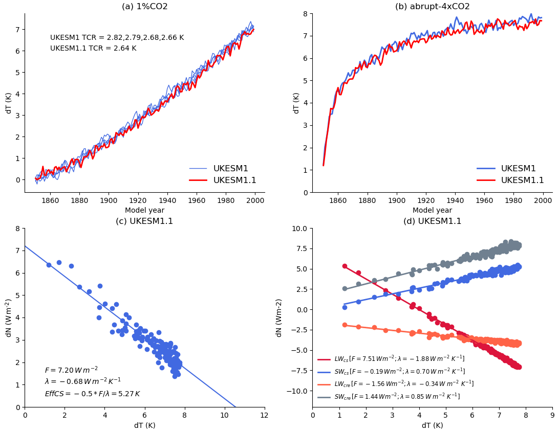
Figure 18Evolution of the global annual mean surface air temperature change in the (a) 1pctCO2 and (b) abrupt-4×CO2 simulations from UKESM1 (blue line) and UKESM1.1 (red line). (c) Regression of the change in net downward radiative flux, N, at the TOA radiation against the change in surface temperature for UKESM1.1. Panel (d) is the same as panel (c) but for the individual SW and LW clear-sky and cloudy-sky components.
The abrupt-4×CO2 and 1pctCO2 simulations are used to calculate the transient climate response (TCR) and effective climate sensitivity (EffCS), using the methodology described in Andrews et al. (2019). As reported by Andrews et al. (2019), the TCR (2.76 K) and EffCS (5.36 K) of UKESM1 are both outside of the CMIP5 5 %–95 % ranges. Figure 18 compares the surface air temperature change in the abrupt-4×CO2 and 1pctCO2 simulations of UKESM1 and UKESM1.1. We note that four ensemble members were run with UKESM1, while only one simulation was run with UKESM1.1 for each experiment. The surface temperature response of the two models is almost identical, at least at the global scale. This leads to values of EffCS (5.27 K) and TCR (2.64 K) for UKESM1.1, which are very similar to those for UKESM1.
Warmer temperatures in response to enhanced CO2 can enhance the emission of natural aerosol sources, such as DMS. Bodas-Salcedo et al. (2019) found that the introduction of the GLOMAP-mode aerosol scheme into the HadGEM3-GC3.1 and UKESM1 models reduces a negative cloud feedback, via a weaker DMS–climate feedback in the Southern Ocean, and this partly contributes to the enhanced climate sensitivity in these models. While the preindustrial background SO4 aerosol is different in UKESM1.1, the dry deposition and DMS chemistry changes will not necessarily change the DMS emission response in the warmer climate.
Andrews et al. (2019) found a notable impact of the biogeochemical feedback from vegetation (via the CO2 fertilisation effect) on the simulated climate response to enhanced CO2 in UKESM1. Large continental increases in surface warming of up to 2 K in the last 50 years of an abrupt-4×CO2 simulation were found due to this effect with the EffCS being 0.3 K higher. The enhanced warming was found to occur predominantly in Northern Hemisphere mid-to-high latitudes, where the CO2 fertilisation effects lead to the expansion of the (less reflective) boreal forests replacing (more reflective) grasses. As these regions have seasonal snow cover, the surface albedo feedback will likely be influenced by the retuning of the snow burial of vegetation parameter (Andrews et al., 2019). Indeed, spatial plots of the decomposed LW and SW clear-sky and cloudy-sky feedbacks (calculated as the local flux change with global mean surface air temperature change; Andrews et al., 2019) indicate a less positive (less amplifying) SW clear-sky feedback across NH continents (Fig. S9). This is offset by a corresponding increase in the LW clear-sky feedback leading to a negligible impact on the net feedback. Overall, the global feedback parameters for the individual components (Fig. 18d) show little change from UKESM1 (see Table 2 in Andrews et al., 2019).
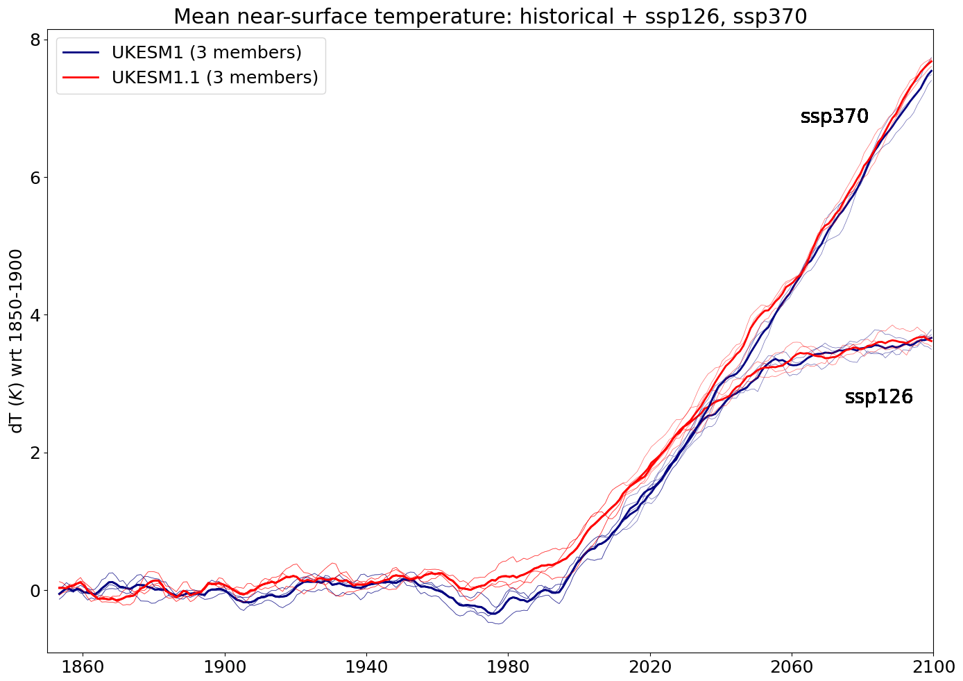
Figure 19Global mean near-surface air temperature anomaly relative to 1850–1900 mean for the historical period and SSP1–2.6 and SSP3–7.0 for UKESM1 (blue) and UKESM1.1 (red). Thick lines are the respective three-member ensemble means and the thin lines are the individual ensemble members.
4.4 Future projections
The response of UKESM1.1 to two future emissions scenarios, SSP1–2.6 and SSP3–7.0, are now examined. Figure 19 shows the global mean near-surface air temperature anomaly for the historical period (1850 to 2014) and the future projection period (2015 to 2100) from UKESM1 and UKESM1.1 for both SSP1–2.6 and SSP3–7.0. Anomalies are calculated relative to a reference period of 1850–1900, and a 5-year running mean has been passed through each time series before the anomalies are calculated.
The differences in the historical period echo what is discussed in Sect. 4.2.1, with UKESM1 exhibiting a stronger cooling between 1940 and 1990 and a slightly stronger global rate of warming after 1990. This behaviour continues into the early period of the projections. Beyond 2040, the differences between the models become negligible, and the temperature time series of the two models become very similar for both SSPs. This highlights the smaller role of SO2 emissions in these specific future climate scenarios.

Figure 20Anomalies in near-surface air temperature expressed as (2070 to 2100 mean) minus (1850 to 1900 mean) for (a, c, e) SSP1–2.6 and (b, d, f) SSP3–7.0, as simulated by (a, b) UKESM1 and (c, d) UKESM1.1. (e, f) UKESM1.1-UKESM1 anomaly differences for each SSP.
Figure 20 presents maps of the near-surface air temperature anomaly calculated as the 2070 to 2100 mean minus the 1850 to 1900 mean, for SSP1–2.6 and SSP3–7.0. Also shown are the differences between the anomalies (UKESM1.1 minus UKESM1). Over most of the globe, differences in the air temperature anomalies are less than ±0.25 K. There is some indication of UKESM1.1 warming less than UKESM1 over the high northern latitudes, with this tendency reversed over the Arctic Ocean and Antarctica. At the beginning of the scenario period, UKESM1.1 has thinner sea ice than UKESM1; hence, the fractional sea ice cover lost in UKESM1.1 will be greater than in UKESM1, driving the slightly increased warming over the majority of historical sea-ice-covered regions (Fig. S10). The slightly reduced warming over Northern Hemisphere land regions in UKESM1.1 may reflect differences in the snow albedo feedback associated with our modification to how the snow burial of vegetation is treated. We note that differences in the anomalies in high-latitude regions are small in comparison to the magnitude of the simulated anomaly itself.
Figure S11 shows the zonal mean precipitation anomalies (2070 to 2100 mean) minus (1850 to 1900 mean) for both SSPs and UKESM configurations. Differences are extremely small, indicating that the two model configurations are largely equivalent in terms of their precipitation sensitivity to future climate change. This is true for both SSPs.
This paper describes and evaluates an updated configuration of UKESM1, which we refer to as UKESM1.1. One of the primary objectives of this work was to investigate if improvements to the parameterisation of SO2 dry deposition, first described in Hardacre et al. (2021), have a significant impact on the large cold bias in the simulated historical global mean surface temperature in the latter half of the 20th century in UKESM1. Aerosols tend to cool the climate and have likely offset a significant fraction of the warming due to increasing greenhouse gases over the historical era. Given the predominant source of aerosols from SO2 emissions during this time, it is reasonable to expect that any changes to SO2 sources or sinks would impact the anthropogenic aerosol forcing, particularly in the late 20th century. While the SO2 dry deposition changes represent the main science change implemented in UKESM1.1, a number of other bug fixes primarily related to aerosols were also included. Furthermore, several tuned parameters in the fully coupled ESM described in Sellar et al. (2019) were revised. The most significant of these include a retuning of the mineral dust scheme to improve the simulation of dust optical depth and a retuning of the extent to which vegetation is buried by snow.
We compare the performance of the historical simulation between UKESM1.1 and UKESM1 using available observations. There is a significant improvement in the evolution of the global mean surface temperature in UKESM1.1, and the large cold bias between 1960 and the late 1980s is reduced by over 50 % in the ensemble mean. Most of the improvement is occurring in the Northern Hemisphere extratropics. A concomitant increase in ocean heat uptake in the Northern Hemisphere oceans, along with lower sea ice extent and volume in the Arctic region, is also found. Regional temperature trends (since 1900) show an overall improvement, although the rate of warming post-1990 is still too high because the climate sensitivity of the model remains largely unchanged. The change in ocean heat content in the top 700 m of the ocean is small, but larger changes (increases) are found through the full ocean depth and are in better agreement with a number of OHC datasets. While the reduced Arctic sea ice is also in better agreement with observations and reanalysis datasets, the high climate sensitivity of both models results in too fast a rate of sea ice loss. Overall, biases and root mean square errors in AOD are improved, and the global reduction in cloud droplet number concentration appears to be in better agreement with the satellite data, although there are large observational uncertainties in this derived quantity. More generally, the UKESM1.1 climate evaluates better or shows neutral changes with respect to UKESM1. For example, minimal changes in ocean circulation are found, while some small variations in ocean productivity are evident, likely driven by a combination of the warmer climate and increased dust deposition.

Figure 21(a) Time series of the historical aerosol ERF from UKESM1 (blue) and UKESM1.1 (red) for all-sky (solid) and clear-sky (dashed lines) conditions. The aerosol ERFs are calculated for selected time slices along the historical period. (b) Interhemispheric gradient in aerosol ERF for each time slice.
The UKESM1.1 model has a larger total anthropogenic ERF (1.84 versus 1.76 W m−2), driven in part by a less negative aerosol ERF (−1.01 versus −1.09 W m−2). The weaker aerosol forcing comes mainly from a smaller clear-sky aerosol scattering contribution, but substantial changes to the background PI climate state driven by changes in both aerosol–cloud and aerosol–radiation interactions are also found. The forcing due to land use change remains largely unchanged, although a weaker clear-sky ERF is found in response to the retuning of the snow burial of vegetation. The model is clearly sensitive to this highly unconstrained parameter, with some regional changes in the climate feedback parameter also found along the marginal snow line. Constraining this parameter using satellite observations of the clear-sky TOA SW radiation reveals a shift from a net positive bias to a net negative bias over the 30 to 60∘ N latitude region in UKESM1.1. So, changes in the future climate response as a consequence of this retuning are possibly exaggerated here, particularly on the regional scales.
The relatively modest change in global mean aerosol ERF between UKESM1 and UKESM1.1, calculated for 2014 anthropogenic aerosol conditions relative to preindustrial period, is unlikely to be the sole explanation of the improved historical temperature response. To obtain a better indication of how the aerosol ERF changed throughout the historical period, we have conducted additional aerosol ERF simulations (piClim-aer) for 1900, 1920, 1950 and 1980 anthropogenic aerosol conditions, in addition to the 2014 simulation. The resulting aerosol ERF time series (Fig. 21) shows that, post-1920, when anthropogenic SO2 emissions start to rapidly increase, the aerosol ERF in UKESM1.1 is consistently less negative in magnitude than UKESM1, with the change in aerosol ERF increasing from +0.01 W m−2 in 1920 to a maximum difference of +0.2 W m−2 in 1980. This change in aerosol ERF is predominantly coming from the Northern Hemisphere, which shows larger changes in aerosol ERF (changing by +0.1 W m−2 in 1920 to +0.31 W m−2 in 1980) than the Southern Hemisphere, leading to a weaker interhemispheric gradient in the aerosol ERF in UKESM1.1 (Fig. 21). This change in the regional pattern of aerosol ERF between UKESM1 and UKESM1.1 could imply that the transient sensitivity to aerosol forcing has changed in UKESM1.1 (Shindell, 2014). The dependence of the transient sensitivity on the forcing is often described as an efficacy (Hansen et al., 2005), and in CMIP6 models, the radiative feedbacks in response to aerosol forcing have been found to be more amplifying (higher transient sensitivity) than that to greenhouse gas forcing (Salvi et al., 2022). We hypothesise that the less negative aerosol forcing over the historical period imposed on a warmer background climate state, which has a less negative SW cloud forcing, is an important factor in the improved simulation of historical surface temperature in UKESM1.1. Our comparison of the effective climate sensitivity and TCR in UKESM1.1 and UKESM1 from the abrupt-4×CO2 and 1pctCO2 simulations shows that the long term-response to CO2 is similar between the two model configurations but is unable to test for a change in transient sensitivity to aerosol forcing. This would require dedicated historical aerosol-only simulations, which is planned in future work. Furthermore, the similarity in the effective climate sensitivity and transient climate response demonstrates that, in this model at least, the effective climate sensitivity does not seem to be related to the magnitude of the aerosol effective radiative forcing or the magnitude of the historical cold temperature bias.
The impact of the model updates implemented in UKESM1.1 on future climate assessed through SSP1–2.6 and SSP3–7.0 is found to be small on the global scale. While only a limited subset of the SSPs were assessed here, using a relatively small ensemble of simulations, the results nevertheless provide some assurance of the continued relevance and value of the more extensive set of scenario projections run with the UKESM1 model for CMIP6.
The historical cold temperature bias has affected many CMIP6 models and not only UKESM1. The magnitude of this bias has caused some concern across the community with respect to the fidelity of these complex global climate models and their ability to realistically simulate future climate change. While we do not necessarily support the heavy weighting applied to a single metric in assessing the skill of an Earth system model, we are interested in understanding the key drivers behind this bias, in particular the role of aerosol. The UKESM1.1 model configuration demonstrates how a seemingly small number of model changes can have a significant impact on the simulated global surface temperature and highlights the complex nature of aerosol feedbacks on historical climate and forcing. This is consistent with the work of Zhang et al. (2021), who demonstrate a strong correlation between sulfate aerosol loading and the global mean surface temperature anomalies across a number of the CMIP6 models.
UKESM1.1 offers a notably improved simulation of several key climate variables compared to the UKESM1 model and fixes a number of bugs that were uncovered in UKESM1. While the EffCS and TCR remain at the upper range of the CMIP6 models, driving too high warming rates in the recent past, the improved simulation of the historical temperature and weaker aerosol forcing will be of interest to many users and scientists.
Table A1Summary of the simulation identifiers used in this study. The branch dates of the piControl simulation are shown in parentheses. The SSPs were branched off of the first three historical simulations listed. Data citations for the model data are also provided.
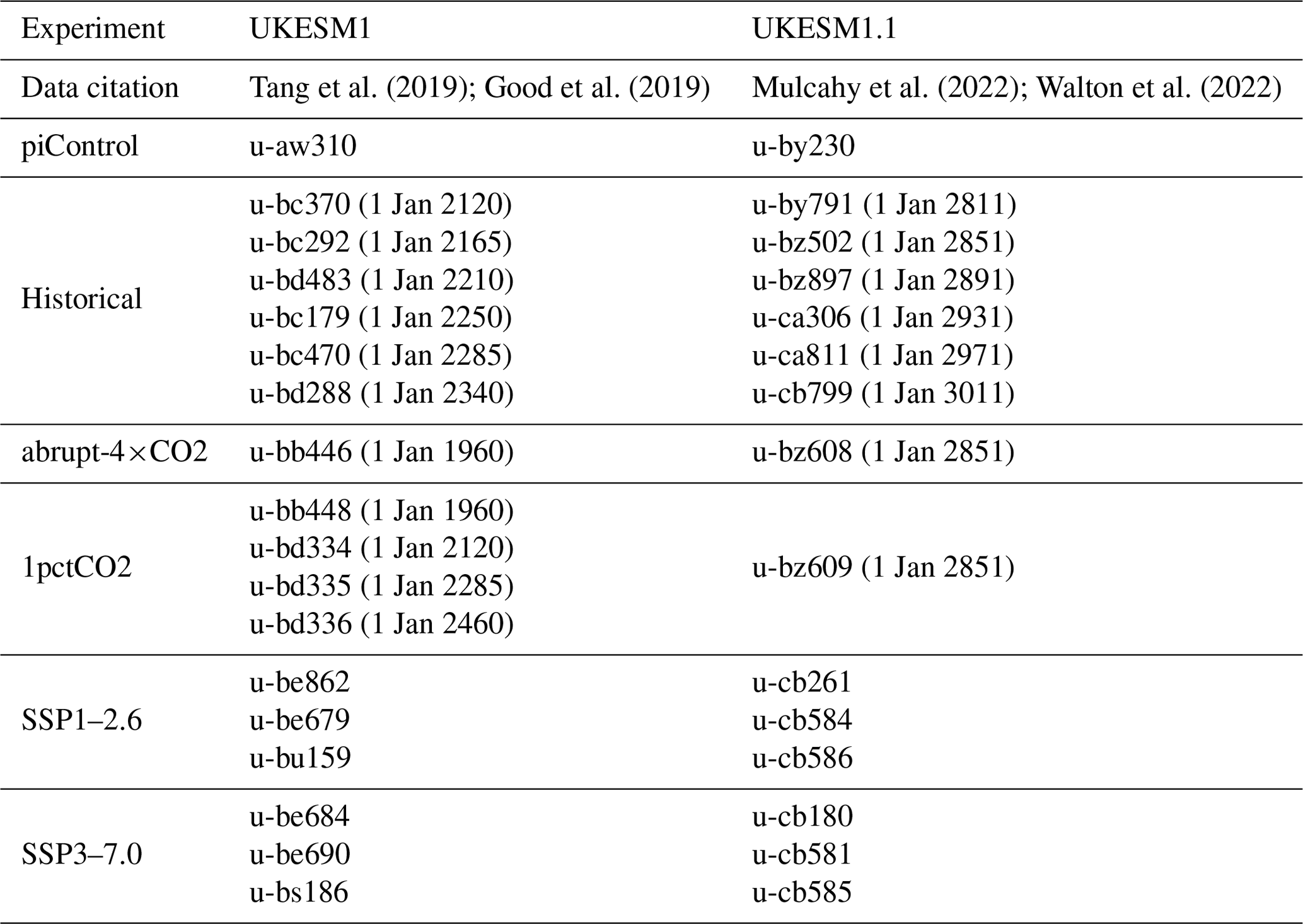
All simulations used in this work were performed using version 11.7 of the Met Office Unified Model (UM), version 5.0 of JULES, NEMO version 3.6, CICE version 5.2.1 and OASIS-MCT version 3.0. The full list of simulation identifiers is provided in Table A1 and details of how to access and run the model can be found at https://cms.ncas.ac.uk/unified-model/configurations/ukesm/relnotes-1.1/ (NCAS Computational Modelling Services, 2023). NEMO is available to download from https://doi.org/10.5281/zenodo.3248739 (Gurvan et al., 2017), and the CICE5 model code used here is available from the Met Office code repository at https://code.metoffice.gov.uk/trac/cice/browser (last access: March 2022; Hunke et al., 2015). Due to intellectual property copyright restrictions, we cannot provide the source code for the UM or JULES, but a copy was made available to the reviewers of this work. The UM is available for use under licence. A number of research organisations and national meteorological services use the UM in collaboration with the Met Office to undertake atmospheric process research, produce forecasts, develop the UM code and build and evaluate Earth system models. To apply for a licence for the UM, go to https://www.metoffice.gov.uk/research/approach/modelling-systems/unified-model (last access: March 2022; Met Office, 2022), and for permission to use JULES, go to https://jules.jchmr.org (last access: March 2022; Walters et al., 2019).
The UKESM1 and UKESM1.1 simulation data used in this study are documented in Table A1 and https://doi.org/10.22033/ESGF/CMIP6.16781 (Mulcahy et al., 2022).
The analysis code and associated model data used to produce the figures in this work are available from https://doi.org/10.5281/zenodo.6535737 (Mulcahy, 2022).
EN.4.2.2 data were obtained from https://www.metoffice.gov.uk/hadobs/en4/ (Good et al., 2013) and are © Crown Copyright, Met Office, 2021, provided under a Non-Commercial Government Licence (http://www.nationalarchives.gov.uk/doc/non-commercial-government-licence/version/2/, last access: March 2023). The HadCRUT5 data were obtained from https://www.metoffice.gov.uk/hadobs/hadcrut5/ (Morice et al., 2021). Satellite-derived AOD data were obtained from ESA CCI (https://catalogue.ceda.ac.uk/uuid/8b63d36f6f1e4efa8aea302b924bc46b, ESA Aerosols CCI project team et al., 2020b; https://catalogue.ceda.ac.uk/uuid/b03b3887ad2f4d5481e7a39344239ab2, ESA Aerosols CCI project team et al., 2020a). MODIS AOD data were obtained from https://earthdata.nasa.gov (last access: 9 February 2022; NASA, 2022). Ground-based AOD data from AERONET are available from https://aeronet.gsfc.nasa.gov/ (last access: 9 February 2022; AERONET, 2022). Cloud droplet number concentration products are available from https://catalogue.ceda.ac.uk/uuid/cf97ccc802d348ec8a3b6f2995dfbbff (Grosvenor, D. P. and Wood, 2018) and https://doi.org/10.15695/vudata.ees.1 (Bennartz and Rausch, 2016, 2017). The RAPID-MOCHA array dataset was obtained from https://doi.org/10.5285/e91b10af-6f0a-7fa7-e053-6c86abc05a09 (Moat et al., 2022)). Dissolved inorganic nitrogen data were obtained from the World Ocean Atlas 2013 https://www.nodc.noaa.gov/OC5/woa13/ (last access: 9 February 2022; (Garcia et al., 2013)). Primary production products (VGPM, Eppley-VGPM and CbPM) were obtained from the Oregon State University Ocean Productivity group at http://sites.science.oregonstate.edu/ocean.productivity/ (last access: 9 February 2022; Ocean Productivity, 2022). Data from the CASTNET (https://www.epa.gov/castnet, last access: 11 February 2022; Clean Air Status and Trends Network, 2022) and EMEP networks (http://ebas.nilu.no/, last access: 11 February 2022; Tørseth et al., 2012) were used in the evaluation of SO2 and SO4 aerosol.
The supplement related to this article is available online at: https://doi.org/10.5194/gmd-16-1569-2023-supplement.
JPM led the development of the UKESM1.1 configuration, the analysis and wrote the paper. CGJ initiated the UKESM1.1 project, led the development of the SO2 dry deposition scheme and made significant contributions to the development and analysis of UKESM1.1. STR coded up the new dry deposition scheme and ran numerous model experiments. TK, AJD, EWB and AY carried out the analysis and made significant contributions to the text. JW, CH, TA and ABS contributed to the figures and/or analysis included in this work. MS, LdM, PH, RH, DK, ER and YT made invaluable contributions to the development of the UKESM1.1 configuration. All co-authors contributed comments on this paper.
At least one of the (co-)authors is a member of the editorial board of Geoscientific Model Development. The peer-review process was guided by an independent editor, and the authors also have no other competing interests to declare.
Publisher's note: Copernicus Publications remains neutral with regard to jurisdictional claims in published maps and institutional affiliations.
We thank Matthew Palmer and Rachel Killick, for their support in obtaining the observational datasets for ocean heat content.
This research has been supported by the Department for Business, Energy and Industrial Strategy, UK Government (Met Office Hadley Centre Climate Programme), the Natural Environment Research Council (grant nos. NE/N017951/1 and NE/N018591/1) and the European Commission H2020 Research Infrastructures (CRESCENDO; grant no. 641816).
This paper was edited by Po-Lun Ma and reviewed by Andrew Gettelman and one anonymous referee.
Aas, W., Mortier, A., Bowersox, V., Cherian, R., Faluvegi, G., Fagerli, H., Hand, J., Klimont, Z., Galy-Lacaux, C., Lehmann, C. M. B., Myhre, C. L., Myhre, G., Olivié, D., Sato, K., Quaas, J., Rao, P. S. P., Schulz, M., Shindell, D., Skeie, R. B., Stein, A., Takemura, T., Tsyro, S., Vet, R., and Xu, X.: Global and regional trends of atmospheric sulfur, Sci. Rep.-UK, 9, 953, https://doi.org/10.1038/s41598-018-37304-0, 2019. a
AERONET: Ground-based AOD data from AERONET, AERONET [data set], https://aeronet.gsfc.nasa.gov/, last access: 9 February 2022. a
Andrews, M. B., Ridley, J. K., Wood, R. A., Andrews, T., Blockley, E. W., Booth, B., Burke, E., Dittus, A. J., Florek, P., Gray, L. J., Haddad, S., Hardiman, S. C., Hermanson, L., Hodson, D., Hogan, E., Jones, G. S., Knight, J. R., Kuhlbrodt, T., Misios, S., Mizielinski, M. S., Ringer, M. A., Robson, J., and Sutton, R. T.: Historical Simulations With HadGEM3-GC3.1 for CMIP6, J. Adv. Model. Earth Sy., 12, e2019MS001995, https://doi.org/10.1029/2019MS001995, 2020. a
Andrews, T., Andrews, M. B., Bodas-Salcedo, A., Jones, G. S., Kuhlbrodt, T., Manners, J., Menary, M. B., Ridley, J., Ringer, M. A., Sellar, A. A., Senior, C. A., and Tang, Y.: Forcings, Feedbacks, and Climate Sensitivity in HadGEM3-GC3.1 and UKESM1, J. Adv. Model. Earth Sy., 11, 4377–4394, https://doi.org/10.1029/2019MS001866, 2019. a, b, c, d, e, f, g
Archibald, A. T., O'Connor, F. M., Abraham, N. L., Archer-Nicholls, S., Chipperfield, M. P., Dalvi, M., Folberth, G. A., Dennison, F., Dhomse, S. S., Griffiths, P. T., Hardacre, C., Hewitt, A. J., Hill, R. S., Johnson, C. E., Keeble, J., Köhler, M. O., Morgenstern, O., Mulcahy, J. P., Ordóñez, C., Pope, R. J., Rumbold, S. T., Russo, M. R., Savage, N. H., Sellar, A., Stringer, M., Turnock, S. T., Wild, O., and Zeng, G.: Description and evaluation of the UKCA stratosphere–troposphere chemistry scheme (StratTrop vn 1.0) implemented in UKESM1, Geosci. Model Dev., 13, 1223–1266, https://doi.org/10.5194/gmd-13-1223-2020, 2020. a, b
Bennartz, R. and Rausch, J.: Cloud Droplet Number Concentration Climatology, Vanderbilt University [data set], https://doi.org/10.15695/vudata.ees.1, 2016. a
Bennartz, R. and Rausch, J.: Global and regional estimates of warm cloud droplet number concentration based on 13 years of AQUA-MODIS observations, Atmos. Chem. Phys., 17, 9815–9836, https://doi.org/10.5194/acp-17-9815-2017, 2017. a, b
Best, M. J., Pryor, M., Clark, D. B., Rooney, G. G., Essery, R. L. H., Ménard, C. B., Edwards, J. M., Hendry, M. A., Porson, A., Gedney, N., Mercado, L. M., Sitch, S., Blyth, E., Boucher, O., Cox, P. M., Grimmond, C. S. B., and Harding, R. J.: The Joint UK Land Environment Simulator (JULES), model description – Part 1: Energy and water fluxes, Geosci. Model Dev., 4, 677–699, https://doi.org/10.5194/gmd-4-677-2011, 2011. a
Bevan, S. L., North, P. R., Los, S. O., and Grey, W. M.: A global dataset of atmospheric aerosol optical depth and surface reflectance from AATSR, Remote Sens. Environ., 116, 199–210, https://doi.org/10.1016/j.rse.2011.05.024, 2012. a
Bodas-Salcedo, A., Mulcahy, J. P., Andrews, T., Williams, K. D., Ringer, M. A., Field, P. R., and Elsaesser, G. S.: Strong Dependence of Atmospheric Feedbacks on Mixed-Phase Microphysics and Aerosol-Cloud Interactions in HadGEM3, J. Adv. Model. Earth Sy., 11, 1735–1758, https://doi.org/10.1029/2019MS001688, 2019. a
Boyer, T., Domingues, C. M., Good, S. A., Johnson, G. C., Lyman, J. M., Ishii, M., Gouretski, V., Willis, J. K., Antonov, J., Wijffels, S., Church, J. A., Cowley, R., and Bindoff, N. L.: Sensitivity of global upper-ocean heat content estimates to mapping methods, XBT bias corrections, and baseline climatologies, J. Climate, 29, 4817–4842, https://doi.org/10.1175/JCLI-D-15-0801.1, 2016. a
Carslaw, K. S., Lee, L. A., Reddington, C. L., Pringle, K. J., Rap, A., Forster, P. M., Mann, G. W., Spracklen, D. V., Woodhouse, M. T., Regayre, L. A., and Pierce, J. R.: Large contribution of natural aerosols to uncertainty in indirect forcing, Nature, 503, 67, https://doi.org/10.1038/nature12674, 2013. a, b
Checa-Garcia, R., Balkanski, Y., Albani, S., Bergman, T., Carslaw, K., Cozic, A., Dearden, C., Marticorena, B., Michou, M., van Noije, T., Nabat, P., O'Connor, F. M., Olivié, D., Prospero, J. M., Le Sager, P., Schulz, M., and Scott, C.: Evaluation of natural aerosols in CRESCENDO Earth system models (ESMs): mineral dust, Atmos. Chem. Phys., 21, 10295–10335, https://doi.org/10.5194/acp-21-10295-2021, 2021. a, b
Cheng, L., Trenberth, K. E., Fasullo, J., Boyer, T., Abraham, J., and Zhu, J.: Improved estimates of ocean heat content from 1960 to 2015, Sci. Adv., 3, 1–11, https://doi.org/10.1126/sciadv.1601545, 2017. a
Cheng, L., Abraham, J., Zhu, J., Trenberth, K. E., Fasullo, J., Boyer, T., Locarnini, R., Zhang, B., Yu, F., Wan, L., Chen, X., Song, X., Liu, Y., and Mann, M. E.: Record-Setting Ocean Warmth Continued in 2019, Adv. Atmos. Sci., 37, 137–142, https://doi.org/10.1007/s00376-020-9283-7, 2020. a
Clark, D. B., Mercado, L. M., Sitch, S., Jones, C. D., Gedney, N., Best, M. J., Pryor, M., Rooney, G. G., Essery, R. L. H., Blyth, E., Boucher, O., Harding, R. J., Huntingford, C., and Cox, P. M.: The Joint UK Land Environment Simulator (JULES), model description – Part 2: Carbon fluxes and vegetation dynamics, Geosci. Model Dev., 4, 701–722, https://doi.org/10.5194/gmd-4-701-2011, 2011. a
Clean Air Status and Trends Network (CASTNET): Aggregate concentration data for weekly sulphur dioxide and weekly sulphate; Historical deposition data for weekly dry deposition of sulphur dioxide and weekly dry deposition of sulphate, CASTNET [data set], http://www.epa.gov/castnet, last access: 11 February 2022. a
Coleman, K. and Jenkinson, D. S.: RothC-26.3: a model for the turnover of carbon in soil. Model description and Users guide, Technical Note, Lawes Agricultural Trust, Harpenden, United Kingdom, 1999. a
Cowtan, K. and Way, R. G.: Coverage bias in the HadCRUT4 temperature series and its impact on recent temperature trends, Q. J. Roy. Meteorol. Soc., 140, 1935–1944, https://doi.org/10.1002/qj.2297, 2014. a, b
Cox, P. M.: Description of the “TRIFFID” dynamic global vegetation model, Hadley Centre Technical Note, Met Office Hadley Centre, Exeter, Devon, United Kingdom, 2001. a
Dittus, A. J., Hawkins, E., Wilcox, L. J., Sutton, R. T., Smith, C. J., Andrews, M. B., and Forster, P. M.: Sensitivity of Historical Climate Simulations to Uncertain Aerosol Forcing, Geophys. Res. Lett., 47, e2019GL085806, https://doi.org/10.1029/2019GL085806, 2020. a
Dittus, A. J., Hawkins, E., Robson, J. I., Smith, D. M., and Wilcox, L. J.: Drivers of Recent North Pacific Decadal Variability: The Role of Aerosol Forcing, Earth's Future, 9, e2021EF002249, https://doi.org/10.1029/2021EF002249, 2021. a
Domingues, C. M., Church, J. A., White, N. J., Gleckler, P. J., Wijffels, S. E., Barker, P. M., and Dunn, J. R.: Improved estimates of upper-ocean warming and multi-decadal sea-level rise, Nature, 453, 1090–1093, https://doi.org/10.1038/nature07080, 2008. a
Donohue, K. A., Tracey, K. L., Watts, D. R., Chidichimo, M. P., and Chereskin, T. K.: Mean Antarctic Circumpolar Current transport measured in Drake Passage, Geophys. Res. Lett., 43, 11760–11767, https://doi.org/10.1002/2016GL070319, 2016. a
Durack, P. J. and Taylor, K. E.: PCMDI AMIP SST and sea-ice boundary conditions version 1.1.3, WCRP [data set], https://doi.org/10.22033/ESGF/input4MIPs.1735, 2017. a
Erisman, J. W. and Baldocchi, D.: Modelling dry deposition of SO2, Tellus B, 46, 159–171, https://doi.org/10.3402/tellusb.v46i3.15789, 1994. a
Erisman, J. W., Van Pul, A., and Wyers, P.: Parametrization of surface resistance for the quantification of atmospheric deposition of acidifying pollutants and ozone, Atmos. Environ., 28, 2595–2607, https://doi.org/10.1016/1352-2310(94)90433-2, 1994. a, b
ESA Aerosols CCI project team, de Leeuw, G., and Popp, T.: ESA Aerosol Climate Change Initiative (Aerosol_cci): Level 2 aerosol products from AATSR (SU Algorithm), Version 4.3, Centre for Environmental Data Analysis, https://catalogue.ceda.ac.uk/uuid/b03b3887ad2f4d5481e7a39344239ab2 (last access: March 2023), 2020a. a
ESA Aerosols CCI project team, de Leeuw, G., and Popp, T.: ESA Aerosol Climate Change Initiative (Aerosol_cci): Level 2 aerosol products from AATSR (ORAC Algorithm), Version 4.01, Centre for Environmental Data Analysis, https://catalogue.ceda.ac.uk/uuid/8b63d36f6f1e4efa8aea302b924bc46b (last access: March 2023), 2020b. a
Eyring, V., Bony, S., Meehl, G. A., Senior, C. A., Stevens, B., Stouffer, R. J., and Taylor, K. E.: Overview of the Coupled Model Intercomparison Project Phase 6 (CMIP6) experimental design and organization, Geosci. Model Dev., 9, 1937–1958, https://doi.org/10.5194/gmd-9-1937-2016, 2016. a, b
Fetterer, F., Knowles, K., Meier, W. N., Savoie, M., and Windnagel, A. K.: Sea Ice Index, Version 3, 1980–2014, https://doi.org/10.7265/N5K072F8 (last access: 10 August 2021), 2017. a
Flynn, C. M. and Mauritsen, T.: On the climate sensitivity and historical warming evolution in recent coupled model ensembles, Atmos. Chem. Phys., 20, 7829–7842, https://doi.org/10.5194/acp-20-7829-2020, 2020. a, b
Forget, G., Campin, J.-M., Heimbach, P., Hill, C. N., Ponte, R. M., and Wunsch, C.: ECCO version 4: an integrated framework for non-linear inverse modeling and global ocean state estimation, Geosci. Model Dev., 8, 3071–3104, https://doi.org/10.5194/gmd-8-3071-2015, 2015. a
Forster, P., Storelvmo, T., Armour, K., Collins, W., Dufresne, J.-L., Frame, D., Lunt, D. J., Mauritsen, T., Palmer, M. D., Watanabe, M., Wild, M., and Zhang, H.: The Earth's Energy Budget, Climate Feedbacks, and Climate Sensitivity, in: Climate Change 2021: The Physical Science Basis. Contribution of Working Group I to the Sixth Assessment Report of the Intergovernmental Panel on Climate Change, edited by: Masson-Delmotte, V., Zhai, P., Pirani, A., Connors, S. L., Péan, C., Berger, S., Caud, N., Chen, Y., Goldfarb, L., Gomis, M. I., Huang, M., Leitzell, K., Lonnoy, E., Matthews, J. B. R., Maycock, T. K., Waterfield, T., Yelekçi, O., Yu, R., and Zhou, B., Cambridge University Press, Cambridge, United Kingdom and New York, NY, USA, 923–1054, https://doi.org/10.1017/9781009157896.009, 2021. a
Fukumori, I., Wang, O., Fenty, I., Forget, G., Heimbach, P., and Ponte, R. M.: Synopsis of the ECCO Central Production Global Ocean and Sea-Ice State Estimate (Version 4 Release 4), Zenodo [data set], https://doi.org/10.5281/zenodo.4533349, 2021. a
Garcia, H. E., Locarnini, R. A., Boyer, T. P., Antonov, J. I., Baranova, O. K., Zweng, M. M., Reagan, J. R., and Johnson, D. R.: Dissolved Inorganic Nutrients (phosphate, nitrate, silicate), in: World Ocean Atlas 2013, edited by: Levitus, S. and Mishonov, A., NOAA Atlas NESDIS 76, Silversprings, Maryland, USA, https://www.nodc.noaa.gov/OC5/woa13/ (last access: 9 February 2022), 2013. a, b
Garland, J. A.: The dry deposition of sulphur dioxide to land and water surfaces, Proc. R. Soc. Land, A, 354, 245–268, https://doi.org/10.1098/rspa.1977.0066, 1977. a
Gent, P. R. and McWilliams, J. C.: Isopycnal mixing in ocean circulation models, J. Phys. Oceanogr., 20, 150–155, https://doi.org/10.1175/1520-0485(1990)020<0150:IMIOCM>2.0.CO;2, 1990. a
Gent, P. R., Willebrand, J., McDougall, T. J., and McWilliams, J. C.: Parameterizing Eddy-Induced Tracer Transports in Ocean Circulation Models, J. Phys. Oceanogr., 25, 463–474, https://doi.org/10.1175/1520-0485(1995)025<0463:PEITTI>2.0.CO;2, 1995. a
Gidden, M. J., Riahi, K., Smith, S. J., Fujimori, S., Luderer, G., Kriegler, E., van Vuuren, D. P., van den Berg, M., Feng, L., Klein, D., Calvin, K., Doelman, J. C., Frank, S., Fricko, O., Harmsen, M., Hasegawa, T., Havlik, P., Hilaire, J., Hoesly, R., Horing, J., Popp, A., Stehfest, E., and Takahashi, K.: Global emissions pathways under different socioeconomic scenarios for use in CMIP6: a dataset of harmonized emissions trajectories through the end of the century, Geosci. Model Dev., 12, 1443–1475, https://doi.org/10.5194/gmd-12-1443-2019, 2019. a, b
Good, P., Sellar, A., Tang, Y., Rumbold, S., Ellis, R., Kelley, D., Kuhlbrodt, T., and Walton, J.: MOHC UKESM1.0-LL model output prepared for CMIP6 ScenarioMIP, WCRP [data set], https://doi.org/10.22033/ESGF/CMIP6.1567, 2019. a
Good, S. A., Martin, M. J., and Rayner, N. A.: EN4: Quality controlled ocean temperature and salinity profiles and monthly objective analyses with uncertainty estimates, J. Geophys. Res.-Oceans, 118, 6704–6716, https://doi.org/10.1002/2013JC009067, 2013 (data available at: https://www.metoffice.gov.uk/hadobs/en4/, last access: March 2023). a, b
Gregory, J. M., Andrews, T., Ceppi, P., Mauritsen, T., and Webb, M. J.: How accurately can the climate sensitivity to CO2 be estimated from historical climate change?, Clim. Dynam., 54, 129–157, https://doi.org/10.1007/s00382-019-04991-y, 2020. a
Grosvenor, D. P. and Wood, R.: Daily MODIS (MODerate Imaging Spectroradiometer) derived cloud droplet number concentration global dataset for 2003–2015, Centre for Environmental Data Analysis, [data set] https://catalogue.ceda.ac.uk/uuid/cf97ccc802d348ec8a3b6f2995dfbbff (last access: March 2023), 2018. a
Grosvenor, D. P., Sourdeval, O., Zuidema, P., Ackerman, A., Alexandrov, M. D., Bennartz, R., Boers, R., Cairns, B., Chiu, J. C., Christensen, M., Deneke, H. M., Diamond, M. S., Feingold, G., Fridlind, A., Hünerbein, A., Knist, C. L., Kollias, P., Marshak, A., McCoy, D., Merk, D., Painemal, D., Rausch, J., Rosenfeld, D., Russchenberg, H., Seifert, P., Sinclair, K., Stier, P., van Diedenhoven, B., Wendisch, M., Werner, F., Wood, R., Zhang, Z., and Quaas, J.: Remote sensing of droplet number concentration in warm clouds: A review of the current state of knowledge and perspectives, Rev. Geophys., 56, 409–453, https://doi.org/10.1029/2017rg000593, 2018. a, b
Gurvan, M., Bourdallé-Badie, R., Bouttier, P.-A., Bricaud, C.,Bruciaferri, D., Calvert, D., Chanut, J., Clementi, E., Coward, A., Delrosso, D., Ethé, C., Flavoni, S., Graham, T., Harle, J., Iovino, D., Lea, D., Lévy, C., Lovato, T., Martin, N., Masson, S., Mocavero, S., Paul, J., Rousset, C., Storkey, D., Storto, A., and Vancoppenolle, M.: NEMO ocean engine, in: Notes du Pôle de modélisation de l'Institut Pierre-Simon Laplace (IPSL) (v3.6-patch, Number 27), Zenodo [data set], https://doi.org/10.5281/zenodo.3248739, 2017. a
Hansen, J., Sato, M., Ruedy, R., Nazarenko, L., Lacis, A., Schmidt, G. A., Russell, G., Aleinov, I., Bauer, M., Bauer, S., Bell, N., Cairns, B., Canuto, V., Chandler, M., Cheng, Y., Del Genio, A., Faluvegi, G., Fleming, E., Friend, A., Hall, T., Jackman, C., Kelley, M., Kiang, N., Koch, D., Lean, J., Lerner, J., Lo, K., Menon, S., Miller, R., Minnis, P., Novakov, T., Oinas, V., Perlwitz, J., Perlwitz, J., Rind, D., Romanou, A., Shindell, D., Stone, P., Sun, S., Tausnev, N., Thresher, D., Wielicki, B., Wong, T., Yao, M., and Zhang, S.: Efficacy of climate forcings, J. Geophys. Res.-Atmos., 110, D18104, https://doi.org/10.1029/2005JD005776, 2005. a
Hardacre, C., Mulcahy, J. P., Pope, R. J., Jones, C. G., Rumbold, S. T., Li, C., Johnson, C., and Turnock, S. T.: Evaluation of SO2, SO and an updated SO2 dry deposition parameterization in the United Kingdom Earth System Model, Atmos. Chem. Phys., 21, 18465–18497, https://doi.org/10.5194/acp-21-18465-2021, 2021. a, b, c, d, e, f, g, h, i, j, k, l
Hill, P. G., Morcrette, C. J., and Boutle, I. A.: A regime-dependent parametrization of subgrid-scale cloud water content variability, Q. J. Roy. Meteor. Soc., 141, 1975–1986, https://doi.org/10.1002/qj.2506, 2015. a
Holben, B. N., Eck, T. F., Slutsker, I., Tanre, D., Buis, J. P., Setzer, A., Vermote, E., Reagan, J. A., Kaufman, Y. J., Nakajima, T., Lavenu, F., Jankowiak, I., and Smirnov, A.: AERONET - A federated instrument network and data archive for aerosol characterization, Remote Sens. Environ., 66, 1–16, 1998. a
Holben, B. N., Tanre, D., Smirnov, A., Eck, T. F., Slutsker, I., Abuhassan, N., Newcomb, W. W., Schafer, J., Chatenet, B., Lavenue, F., Kaufman, Y. J., Castle, J. V., Setzer, A., Markham, B., Clark, D., Frouin, R., Halthore, R., Karnieli, A., O'Neill, N. T., Pietras, C., Pinker, R. T., Voss, K., and Zibordi, G.: An emerging ground-based aerosol climatology: Aerosol Optical Depth from AERONET, J. Geophys. Res., 106, 12067–12097, 2001. a
Hourdin, F., Mauritsen, T., Gettelman, A., Golaz, J.-C., Balaji, V., Duan, Q., Folini, D., Ji, D., Klocke, D., Qian, Y., Rauser, F., Rio, C., Tomassini, L., Watanabe, M., and Williamson, D.: The Art and Science of Climate Model Tuning, B. Am. Meteorol. Soc., 98, 589–602, https://doi.org/10.1175/BAMS-D-15-00135.1, 2017. a
Hsu, N. C., Tsay, S. C., King, M. D., and Herman, J. R.: Aerosol Properties over Bright-Reflecting Source Regions, IEEE T. Geosci. Remote, 42, 557–569, 2004. a
Hunke, E. C., Lipscomb, W. H., Turner, A. K., Jeffery, N., and Elliott, S.: CICE: the Los Alamos Sea Ice Model Documentation and Software User's Manual Version 5.1, LA-CC-06-012, Los Alamos National Laboratory, Los Alamos, NM [code], https://code.metoffice.gov.uk/trac/cice/browser (last access: March 2022), 2015. a
Ishii, M., Fukuda, Y., Hirahara, S., Yasui, S., Suzuki, T., and Sato, K.: Accuracy of Global Upper Ocean Heat Content Estimation Expected from Present Observational Data Sets, SOLA, 13, 163–167, https://doi.org/10.2151/sola.2017-030, 2017. a
Jones, C. D., Arora, V., Friedlingstein, P., Bopp, L., Brovkin, V., Dunne, J., Graven, H., Hoffman, F., Ilyina, T., John, J. G., Jung, M., Kawamiya, M., Koven, C., Pongratz, J., Raddatz, T., Randerson, J. T., and Zaehle, S.: C4MIP – The Coupled Climate–Carbon Cycle Model Intercomparison Project: experimental protocol for CMIP6, Geosci. Model Dev., 9, 2853–2880, https://doi.org/10.5194/gmd-9-2853-2016, 2016. a, b
Kiehl, J. T.: Twentieth century climate model response and climate sensitivity, Geophys. Res. Lett., 34, L22710, https://doi.org/10.1029/2007GL031383, 2007. a
Kuhlbrodt, T., Jones, C. G., Sellar, A., Storkey, D., Blockley, E., Stringer, M., Hill, R., Graham, T., Ridley, J., Blaker, A., Calvert, D., Copsey, D., Ellis, R., Hewitt, H., Hyder, P., Ineson, S., Mulcahy, J., Siahaan, A., and Walton, J.: The Low-Resolution Version of HadGEM3 GC3.1: Development and Evaluation for Global Climate, J. Adv. Model. Earth Sy., 10, 2865–2888, https://doi.org/10.1029/2018MS001370, 2018. a, b, c, d
Levitus, S., Antonov, J. I., Boyer, T. P., Baranova, O. K., Garcia, H. E., Locarnini, R. A., Mishonov, A. V., Reagan, J. R., Seidov, D., Yarosh, E. S., and Zweng, M. M.: World ocean heat content and thermosteric sea level change (0–2000 m), 1955–2010, Geophys. Res. Lett., 39, L10603, https://doi.org/10.1029/2012GL051106, 2012. a, b
Mahlstein, I. and Knutti, R.: September Arctic sea ice predicted to disappear near 2 ∘C global warming above present, J. Geophys. Res., 117, D06104, https://doi.org/10.1029/2011JD016709, 2012. a
Mahowald, N. M., Baker, A. R., Bergametti, G., Brooks, N., Duce, R. A., Jickells, T. D., Kubilay, N., Prospero, J. M., and Tegen, I.: Atmospheric global dust cycle and iron inputs to the ocean, Global Biogeochem. Cycles, 19, GB4025, https://doi.org/10.1029/2004GB002402, 2005. a
Mauritsen, T. and Roeckner, E.: Tuning the MPI-ESM1.2 Global Climate Model to Improve the Match With Instrumental Record Warming by Lowering Its Climate Sensitivity, J. Adv. Model. Earth Sy., 12, e2019MS002037, https://doi.org/10.1029/2019MS002037, 2020. a
McDuffie, E. E., Smith, S. J., O'Rourke, P., Tibrewal, K., Venkataraman, C., Marais, E. A., Zheng, B., Crippa, M., Brauer, M., and Martin, R. V.: A global anthropogenic emission inventory of atmospheric pollutants from sector- and fuel-specific sources (1970–2017): an application of the Community Emissions Data System (CEDS), Earth Syst. Sci. Data, 12, 3413–3442, https://doi.org/10.5194/essd-12-3413-2020, 2020. a
Menary, M. B., Roberts, C. D., Palmer, M. D., Halloran, P. R., Jackson, L., Wood, R. A., Müller, W. A., Matei, D., and Lee, S.-K.: Mechanisms of aerosol-forced AMOC variability in a state of the art climate model, J. Geophys. Res.-Oceans, 118, 2087–2096, https://doi.org/10.1002/jgrc.20178, 2013. a
Menary, M. B., Kuhlbrodt, T., Ridley, J., Andrews, M. B., Dimdore-Miles, O. B., Deshayes, J., Eade, R., Gray, L., Ineson, S., Mignot, J., Roberts, C. D., Robson, J., Wood, R. A., and Xavier, P.: Preindustrial Control Simulations With HadGEM3-GC3.1 for CMIP6, J. Adv. Model. Earth Sy., 10, 3049–3075, https://doi.org/10.1029/2018MS001495, 2018. a
Menary, M. B., Robson, J., Allan, R. P., Booth, B. B. B., Cassou, C., Gastineau, G., Gregory, J., Hodson, D., Jones, C., Mignot, J., Ringer, M., Sutton, R., Wilcox, L., and Zhang, R.: Aerosol-Forced AMOC Changes in CMIP6 Historical Simulations, Geophys. Res. Lett., 47, e2020GL088166, https://doi.org/10.1029/2020GL088166, 2020. a
Met Office: Unified Model, https://www.metoffice.gov.uk/research/approach/modelling-systems/unified-model, last access: March 2022. a
Moat, B. I., Frajka-Williams, E., Smeed, D. A., Rayner, D., Johns, W. E., Baringer, M. O., Volkov, D., and Collins, J.: Atlantic meridional overturning circulation observed by the RAPID-MOCHA-WBTS (RAPID-Meridional Overturning Circulation and Heatflux Array-Western Boundary Time Series) array at 26N from 2004 to 2020 (v2020.2), British Oceanographic Data Centre – Natural Environment Research Council, UK [data set], https://doi.org/10.5285/e91b10af-6f0a-7fa7-e053-6c86abc05a09, 2022. a
Morice, C. P., Kennedy, J. J., Rayner, N. A., Winn, J. P., Hogan, E., Killick, R. E., Dunn, R. J. H., Osborn, T. J., Jones, P. D., and Simpson, I. R.: An Updated Assessment of Near-Surface Temperature Change From 1850: The HadCRUT5 Data Set, J. Geophys. Res.-Atmos., 126, e2019JD032361, https://doi.org/10.1029/2019JD032361, 2021 (data available at: https://www.metoffice.gov.uk/hadobs/hadcrut5/, last access: 11 November 2021). a, b, c, d, e
Mulcahy, J., S., R., Y., T., Walton, J., Hardacre, C., Stringer, M., Hill, R., Kuhlbrodt, T., and Jones, C.: MOHC UKESM1.1-LL model output prepared for CMIP6 CMIP. Version 20220624, WCRP [data set], https://doi.org/10.22033/ESGF/CMIP6.16781, 2022. a, b
Mulcahy, J. P.: Supplementary material for manuscript “UKESM1.1: Development and evaluation of an updated configuration of the UK Earth System Model”, Zenodo [code], https://doi.org/10.5281/zenodo.6535737, 2022. a
Mulcahy, J. P., Jones, C., Sellar, A., Johnson, B., Boutle, I. A., Jones, A., Andrews, T., Rumbold, S. T., Mollard, J., Bellouin, N., Johnson, C. E., Williams, K. D., Grosvenor, D. P., and McCoy, D. T.: Improved Aerosol Processes and Effective Radiative Forcing in HadGEM3 and UKESM1, J. Adv. Model. Earth Sy., 10, 2786–2805, https://doi.org/10.1029/2018MS001464, 2018. a, b, c
Mulcahy, J. P., Johnson, C., Jones, C. G., Povey, A. C., Scott, C. E., Sellar, A., Turnock, S. T., Woodhouse, M. T., Abraham, N. L., Andrews, M. B., Bellouin, N., Browse, J., Carslaw, K. S., Dalvi, M., Folberth, G. A., Glover, M., Grosvenor, D. P., Hardacre, C., Hill, R., Johnson, B., Jones, A., Kipling, Z., Mann, G., Mollard, J., O'Connor, F. M., Palmiéri, J., Reddington, C., Rumbold, S. T., Richardson, M., Schutgens, N. A. J., Stier, P., Stringer, M., Tang, Y., Walton, J., Woodward, S., and Yool, A.: Description and evaluation of aerosol in UKESM1 and HadGEM3-GC3.1 CMIP6 historical simulations, Geosci. Model Dev., 13, 6383–6423, https://doi.org/10.5194/gmd-13-6383-2020, 2020. a, b, c, d, e, f, g, h, i, j, k
NASA: NASA Earth data, https://earthdata.nasa.gov, last access: 9 February 2022. a
NCAS Computational Modelling Services: UKESM1.1 Release Notes, https://cms.ncas.ac.uk/unified-model/configurations/ukesm/relnotes-1.1/, last access: 6 March 2023. a
Ocean Productivity: Welcome to the Ocean Productivity Home Page, Ocean Productivity [data set], http://sites.science.oregonstate.edu/ocean.productivity/, last access: 9 February 2022. a
O'Connor, F. M., Johnson, C. E., Morgenstern, O., Abraham, N. L., Braesicke, P., Dalvi, M., Folberth, G. A., Sanderson, M. G., Telford, P. J., Voulgarakis, A., Young, P. J., Zeng, G., Collins, W. J., and Pyle, J. A.: Evaluation of the new UKCA climate-composition model – Part 2: The Troposphere, Geosci. Model Dev., 7, 41–91, https://doi.org/10.5194/gmd-7-41-2014, 2014. a
O'Connor, F. M., Abraham, N. L., Dalvi, M., Folberth, G. A., Griffiths, P. T., Hardacre, C., Johnson, B. T., Kahana, R., Keeble, J., Kim, B., Morgenstern, O., Mulcahy, J. P., Richardson, M., Robertson, E., Seo, J., Shim, S., Teixeira, J. C., Turnock, S. T., Williams, J., Wiltshire, A. J., Woodward, S., and Zeng, G.: Assessment of pre-industrial to present-day anthropogenic climate forcing in UKESM1, Atmos. Chem. Phys., 21, 1211–1243, https://doi.org/10.5194/acp-21-1211-2021, 2021. a, b
Oki, T. and Sud, Y. C.: Design of Total Runoff Integrating Pathways (TRIP) – A Global River Channel Network, Earth Interactions, 2, 1–37, https://doi.org/10.1175/1087-3562(1998)002<0001:DOTRIP>2.3.CO;2, 1998. a
O'Neill, B. C., Tebaldi, C., van Vuuren, D. P., Eyring, V., Friedlingstein, P., Hurtt, G., Knutti, R., Kriegler, E., Lamarque, J.-F., Lowe, J., Meehl, G. A., Moss, R., Riahi, K., and Sanderson, B. M.: The Scenario Model Intercomparison Project (ScenarioMIP) for CMIP6, Geosci. Model Dev., 9, 3461–3482, https://doi.org/10.5194/gmd-9-3461-2016, 2016. a
Pincus, R., Forster, P. M., and Stevens, B.: The Radiative Forcing Model Intercomparison Project (RFMIP): experimental protocol for CMIP6, Geosci. Model Dev., 9, 3447–3460, https://doi.org/10.5194/gmd-9-3447-2016, 2016. a, b, c
Purkey, S. G. and Johnson, G. C.: Warming of global abyssal and deep Southern Ocean waters between the 1990s and 2000s: Contributions to global heat and sea level rise budgets, J. Climate, 23, 6336–6351, https://doi.org/10.1175/2010JCLI3682.1, 2010. a
Ranjithkumar, A., Gordon, H., Williamson, C., Rollins, A., Pringle, K., Kupc, A., Abraham, N. L., Brock, C., and Carslaw, K.: Constraints on global aerosol number concentration, SO2 and condensation sink in UKESM1 using ATom measurements, Atmos. Chem. Phys., 21, 4979–5014, https://doi.org/10.5194/acp-21-4979-2021, 2021. a
Revell, L. E., Kremser, S., Hartery, S., Harvey, M., Mulcahy, J. P., Williams, J., Morgenstern, O., McDonald, A. J., Varma, V., Bird, L., and Schuddeboom, A.: The sensitivity of Southern Ocean aerosols and cloud microphysics to sea spray and sulfate aerosol production in the HadGEM3-GA7.1 chemistry–climate model, Atmos. Chem. Phys., 19, 15447–15466, https://doi.org/10.5194/acp-19-15447-2019, 2019. a
Richter, J. H., Anstey, J. A., Butchart, N., Kawatani, Y., Meehl, G. A., Osprey, S., and Simpson, I. R.: Progress in Simulating the Quasi-Biennial Oscillation in CMIP Models, J. Geophys. Res.-Atmos., 125, e2019JD032362, https://doi.org/10.1029/2019JD032362, 2020. a
Ridley, J. K., Blockley, E. W., Keen, A. B., Rae, J. G. L., West, A. E., and Schroeder, D.: The sea ice model component of HadGEM3-GC3.1, Geosci. Model Dev., 11, 713–723, https://doi.org/10.5194/gmd-11-713-2018, 2018. a
Robson, J., Aksenov, Y., Bracegirdle, T. J., Dimdore-Miles, O., Griffiths, P. T., Grosvenor, D. P., Hodson, D. L. R., Keeble, J., MacIntosh, C., Megann, A., Osprey, S., Povey, A. C., Schröder, D., Yang, M., Archibald, A. T., Carslaw, K. S., Gray, L., Jones, C., Kerridge, B., Knappett, D., Kuhlbrodt, T., Russo, M., Sellar, A., Siddans, R., Sinha, B., Sutton, R., Walton, J., and Wilcox, L. J.: The Evaluation of the North Atlantic Climate System in UKESM1 Historical Simulations for CMIP6, J. Adv. Model. Earth Sy., 12, e2020MS002126, https://doi.org/10.1029/2020MS002126, 2020. a, b
Rosenblum, E. and Eisenman, I.: Sea ice trends in climate models only accurate in run with biased global warming, J. Climate, 30, 6265–6278, https://doi.org/10.1175/JCLI-D-16-0455.1, 2017. a
Salvi, P., Ceppi, P., and Gregory, J. M.: Interpreting Differences in Radiative Feedbacks From Aerosols Versus Greenhouse Gases, Geophys. Res. Lett., 49, e2022GL097766, https://doi.org/10.1029/2022GL097766, 2022. a
Schmidt, G. A., Bader, D., Donner, L. J., Elsaesser, G. S., Golaz, J.-C., Hannay, C., Molod, A., Neale, R. B., and Saha, S.: Practice and philosophy of climate model tuning across six US modeling centers, Geosci. Model Dev., 10, 3207–3223, https://doi.org/10.5194/gmd-10-3207-2017, 2017. a
Schweiger, A., Lindsay, R., Zhang, J., Steele, M., Stern, H., and Kwok, R.: Uncertainty in modeled Arctic sea ice volume, J. Geophys. Res.-Oceans, 116, C00D06, https://doi.org/10.1029/2011JC007084, 2011. a
Sellar, A. A., Jones, C. G., Mulcahy, J. P., Tang, Y., Yool, A., Wiltshire, A., O'Connor, F. M., Stringer, M., Hill, R., Palmieri, J., Woodward, S., de Mora, L., Kuhlbrodt, T., Rumbold, S., Kelley, D. I., Ellis, R., Johnson, C. E., Walton, J., Abraham, N. L., Andrews, M. B., Andrews, T., Archibald, A. T., Berthou, S., Burke, E., Blockley, E., Carslaw, K., Dalvi, M., Edwards, J., Folberth, G. A., Gedney, N., Griffiths, P. T., Harper, A. B., Hendry, M. A., Hewitt, A. J., Johnson, B., Jones, A., Jones, C. D., Keeble, J., Liddicoat, S., Morgenstern, O., Parker, R. J., Predoi, V., Robertson, E., Siahaan, A., Smith, R. S., Swaminathan, R., Woodhouse, M., Zeng, G., and Zerroukat, M.: UKESM1: Description and evaluation of the UK Earth System Model, J. Adv. Model. Earth Sy., 11, 4513–4558, https://doi.org/10.1029/2019MS001739, 2019. a, b, c, d, e, f, g, h, i, j, k, l, m, n, o, p, q
Sellar, A. A., Walton, J., Jones, C. G., Wood, R., Abraham, N. L., Andrejczuk, M., Andrews, M. B., Andrews, T., Archibald, A. T., de Mora, L., Dyson, H., Elkington, M., Ellis, R., Florek, P., Good, P., Gohar, L., Haddad, S., Hardiman, S. C., Hogan, E., Iwi, A., Jones, C. D., Johnson, B., Kelley, D. I., Kettleborough, J., Knight, J. R., Köhler, M. O., Kuhlbrodt, T., Liddicoat, S., Linova-Pavlova, I., Mizielinski, M. S., Morgenstern, O., Mulcahy, J., Neininger, E., O'Connor, F. M., Petrie, R., Ridley, J., Rioual, J.-C., Roberts, M., Robertson, E., Rumbold, S., Seddon, J., Shepherd, H., Shim, S., Stephens, A., Teixiera, J. C., Tang, Y., Williams, J., Wiltshire, A., and Griffiths, P. T.: Implementation of U.K. Earth System Models for CMIP6, J. Adv. Model. Earth Sy., 12, e2019MS001946, https://doi.org/10.1029/2019MS001946, 2020. a
Senior, C. A., Jones, C. G., Wood, R. A., Sellar, A., Belcher, S., Klein-Tank, A., Sutton, R., Walton, J., Lawrence, B., Andrews, T., and Mulcahy, J. P.: U.K. Community Earth System Modeling for CMIP6, J. Adv. Model. Earth Sy., 12, e2019MS002004, https://doi.org/10.1029/2019MS002004, 2020. a
Shindell, D. T.: Inhomogeneous forcing and transient climate sensitivity, Nat. Clim. Change, 4, 274–277, https://doi.org/10.1038/nclimate2136, 2014. a
Smeed, D. A., Josey, S. A., Beaulieu, C., Johns, W. E., Moat, B. I., Frajka-Williams, E., Rayner, D., Meinen, C. S., Baringer, M. O., Bryden, H. L., and McCarthy, G. D.: The North Atlantic Ocean Is in a State of Reduced Overturning, Geophys. Res. Lett., 45, 1527–1533, https://doi.org/10.1002/2017GL076350, 2018. a, b
Smith, F. and Jeffrey, G.: Airborne transport of sulphur dioxide from the U.K., Atmos. Environ., 9, 643–659, https://doi.org/10.1016/0004-6981(75)90008-6, 1975. a
Storkey, D., Blaker, A. T., Mathiot, P., Megann, A., Aksenov, Y., Blockley, E. W., Calvert, D., Graham, T., Hewitt, H. T., Hyder, P., Kuhlbrodt, T., Rae, J. G. L., and Sinha, B.: UK Global Ocean GO6 and GO7: a traceable hierarchy of model resolutions, Geosci. Model Dev., 11, 3187–3213, https://doi.org/10.5194/gmd-11-3187-2018, 2018. a
Tang, Y., Rumbold, S., Ellis, R., Kelley, D., Mulcahy, J., Sellar, A., Walton, J., and Jones, C.: MOHC UKESM1.0-LL model output prepared for CMIP6 CMIP, WCRP [data set], https://doi.org/10.22033/ESGF/CMIP6.1569, 2019. a
Taylor, K. E., Crucifix, M., Braconnot, P., Hewitt, C. D., Doutriaux, C., Broccoli, A. J., Mitchell, J. F. B., and Webb, M. J.: Estimating Shortwave Radiative Forcing and Response in Climate Models, J. Climate, 20, 2530–2543, https://doi.org/10.1175/JCLI4143.1, 2007. a
Thomas, G. E., Poulsen, C. A., Sayer, A. M., Marsh, S. H., Dean, S. M., Carboni, E., Siddans, R., Grainger, R. G., and Lawrence, B. N.: The GRAPE aerosol retrieval algorithm, Atmos. Meas. Tech., 2, 679–701, https://doi.org/10.5194/amt-2-679-2009, 2009. a
Titchner, H. A. and Rayner, N. A.: The Met Office Hadley Centre sea ice and sea surface temperature data set, version 2: 1. Sea ice concentrations, J. Geophys. Res.-Atmos., 119, 2864–2889, https://doi.org/10.1002/2013JD020316, 2014. a
Tørseth, K., Aas, W., Breivik, K., Fjæraa, A. M., Fiebig, M., Hjellbrekke, A. G., Lund Myhre, C., Solberg, S., and Yttri, K. E.: Introduction to the European Monitoring and Evaluation Programme (EMEP) and observed atmospheric composition change during 1972–2009, Atmos. Chem. Phys., 12, 5447–5481, https://doi.org/10.5194/acp-12-5447-2012, 2012 (data available at: http://ebas.nilu.no/, last access: 11 February 2022). a
von Schuckmann, K., Palmer, M. D., Trenberth, K. E., Cazenave, A., Chambers, D., Champollion, N., Hansen, J., Josey, S. A., Loeb, N., Mathieu, P. P., Meyssignac, B., and Wild, M.: An imperative to monitor Earth's energy imbalance, Nat. Clim. Change, 6, 138–144, https://doi.org/10.1038/nclimate2876, 2016. a
Walters, D., Baran, A. J., Boutle, I., Brooks, M., Earnshaw, P., Edwards, J., Furtado, K., Hill, P., Lock, A., Manners, J., Morcrette, C., Mulcahy, J., Sanchez, C., Smith, C., Stratton, R., Tennant, W., Tomassini, L., Van Weverberg, K., Vosper, S., Willett, M., Browse, J., Bushell, A., Carslaw, K., Dalvi, M., Essery, R., Gedney, N., Hardiman, S., Johnson, B., Johnson, C., Jones, A., Jones, C., Mann, G., Milton, S., Rumbold, H., Sellar, A., Ujiie, M., Whitall, M., Williams, K., and Zerroukat, M.: The Met Office Unified Model Global Atmosphere 7.0/7.1 and JULES Global Land 7.0 configurations, Geosci. Model Dev., 12, 1909–1963, https://doi.org/10.5194/gmd-12-1909-2019, 2019 (code available at: https://jules.jchmr.org, last access: March 2022). a, b
Walters, D. N., Williams, K. D., Boutle, I. A., Bushell, A. C., Edwards, J. M., Field, P. R., Lock, A. P., Morcrette, C. J., Stratton, R. A., Wilkinson, J. M., Willett, M. R., Bellouin, N., Bodas-Salcedo, A., Brooks, M. E., Copsey, D., Earnshaw, P. D., Hardiman, S. C., Harris, C. M., Levine, R. C., MacLachlan, C., Manners, J. C., Martin, G. M., Milton, S. F., Palmer, M. D., Roberts, M. J., Rodríguez, J. M., Tennant, W. J., and Vidale, P. L.: The Met Office Unified Model Global Atmosphere 4.0 and JULES Global Land 4.0 configurations, Geosci. Model Dev., 7, 361–386, https://doi.org/10.5194/gmd-7-361-2014, 2014. a
Walton, J., Mulcahy, J., Tang, Y., Rumbold, S., Hardacre, C., Stringer, M., Hill, R., Kuhlbrodt, T., and Jones, C.: MOHC UKESM1.1-LL model output prepared for CMIP6 ScenarioMIP, WCRP [data set], https://doi.org/10.22033/ESGF/CMIP6.16782, 2022. a
Wesely, M.: Parameterization of surface resistances to gaseous dry deposition in regional-scale numerical models, Atmos. Environ., 23, 1293–1304, 1989. a
West, R. E. L., Stier, P., Jones, A., Johnson, C. E., Mann, G. W., Bellouin, N., Partridge, D. G., and Kipling, Z.: The importance of vertical velocity variability for estimates of the indirect aerosol effects, Atmos. Chem. Phys., 14, 6369–6393, https://doi.org/10.5194/acp-14-6369-2014, 2014. a
Williams, K. D., Copsey, D., Blockley, E. W., Bodas-Salcedo, A., Calvert, D., Comer, R., Davis, P., Graham, T., Hewitt, H. T., Hill, R., Hyder, P., Ineson, S., Johns, T. C., Keen, A. B., Lee, R. W., Megann, A., Milton, S. F., Rae, J. G. L., Roberts, M. J., Scaife, A. A., Schiemann, R., Storkey, D., Thorpe, L., Watterson, I. G., Walters, D. N., West, A., Wood, R. A., Woollings, T., and Xavier, P. K.: The Met Office Global Coupled Model 3.0 and 3.1 (GC3.0 and GC3.1) Configurations, J. Adv. Model. Earth Sy., 10, 357–380, https://doi.org/10.1002/2017MS001115, 2017. a, b
Woodward, S.: Modelling the atmospheric life cycle and radiative impact of mineral dust in the Hadley Centre climate model, J. Geophys. Res., 106, 18155–18166, 2001. a
Woodward, S.: Mineral dust in HadGEM2, Hadley Centre Technical Note 87, Met Office Hadley Centre, Exeter, Devon, United Kingdom, 2011. a
Wys, J. N. D., Hill, A., and Robinson, E.: Assessment of the fate of Sulphur Dioxide from a point source, in: Sulfur in the Atmosphere, edited by: HUSAR, R., LODGE, J., and MOORE, D., Pergamon, 633–639, https://doi.org/10.1016/B978-0-08-022932-4.50065-3, 1978. a
Yool, A., Popova, E. E., and Anderson, T. R.: MEDUSA-2.0: an intermediate complexity biogeochemical model of the marine carbon cycle for climate change and ocean acidification studies, Geosci. Model Dev., 6, 1767–1811, https://doi.org/10.5194/gmd-6-1767-2013, 2013. a, b
Yool, A., Palmieri, J., Jones, C. G., Sellar, A. A., de Mora, L., Kuhlbrodt, T., Popova, E. E., Mulcahy, J., Wiltshire, A., Rumbold, S. T., Stringer, M., Hill, R., Tang, Y., Walton, J., Blaker, A., Nurser, A. J. G., Coward, A. C., Hirschi, J., Woodward, S., Kelley, D. I., and Ellis, R.: Spin-up of UK Earth System Model 1 (UKESM1) for CMIP6, J. Adv. Model. Earth Sy., 12, e2019MS001933, https://doi.org/10.1029/2019MS001933, 2019. a
Yool, A., Palmiéri, J., Jones, C. G., de Mora, L., Kuhlbrodt, T., Popova, E. E., Nurser, A. J. G., Hirschi, J., Blaker, A. T., Coward, A. C., Blockley, E. W., and Sellar, A. A.: Evaluating the physical and biogeochemical state of the global ocean component of UKESM1 in CMIP6 historical simulations, Geosci. Model Dev., 14, 3437–3472, https://doi.org/10.5194/gmd-14-3437-2021, 2021. a, b, c, d
Zelinka, M. D., Andrews, T., Forster, P., and Taylor, K. E.: Quantifying components of aerosol-cloud-radiation interactions in climate models, J. Geophys. Res.-Atmos., 119, 7599–7615, https://doi.org/10.1002/2014JD021710, 2014. a
Zhang, J., Furtado, K., Turnock, S. T., Mulcahy, J. P., Wilcox, L. J., Booth, B. B., Sexton, D., Wu, T., Zhang, F., and Liu, Q.: The role of anthropogenic aerosols in the anomalous cooling from 1960 to 1990 in the CMIP6 Earth system models, Atmos. Chem. Phys., 21, 18609–18627, https://doi.org/10.5194/acp-21-18609-2021, 2021. a, b, c
Zhang, L., Brook, J. R., and Vet, R.: A revised parameterization for gaseous dry deposition in air-quality models, Atmos. Chem. Phys., 3, 2067–2082, https://doi.org/10.5194/acp-3-2067-2003, 2003. a
- Abstract
- Copyright statement
- Introduction
- Model description
- Model simulations
- Results
- Discussion and conclusions
- Appendix A: Simulation and model data information
- Code and data availability
- Author contributions
- Competing interests
- Disclaimer
- Acknowledgements
- Financial support
- Review statement
- References
- Supplement