Deep learning models for generation of precipitation maps based on numerical weather prediction

Numerical weather prediction (NWP) models are atmospheric simulations that imitate the dynamics of the atmosphere and provide high-quality forecasts. One of the most significant limitations of NWP is the elevated amount of computational resources required for its functioning, which limits the spatial and temporal resolution of the outputs. Traditional meteorological techniques to increase the resolution are uniquely based on information from a limited group of interest variables. In this study, we offer an alternative approach to the task where we generate precipitation maps based on the complete set of variables of the NWP to generate high-resolution and short-time precipitation predictions. To achieve this, five different deep learning models were trained and evaluated: a baseline, U-Net, two deconvolution networks and one conditional generative model (Conditional Generative Adversarial Network; CGAN). A total of 20 independent random initializations were performed for each of the models. The predictions were evaluated using skill scores based on mean absolute error (MAE) and linear error in probability space (LEPS), equitable threat score (ETS), critical success index (CSI) and frequency bias after applying several thresholds. The models showed a significant improvement in predicting precipitation, showing the benefits of including the complete information from the NWP. The algorithms doubled the resolution of the predictions and corrected an over-forecast bias from the input information. However, some new models presented new types of bias: U-Net tended to mid-range precipitation events, and the deconvolution models favored low rain events and generated some spatial smoothing. The CGAN offered the highest-quality precipitation forecast, generating realistic outputs and indicating possible future research paths.

1 Introduction

Precipitation prediction is a fundamental scientific and social problem. Accurate rain forecasts play a crucial role in sectors like agriculture, energy, transportation and recreation and help to prevent human and material losses in extreme weather events such as floods or storms. Nevertheless, it remains an unsolved problem due to its high complexity, the large number of atmospheric variables involved, and the complex interactions between them. This complexity and the rarity of high precipitation events make it a challenging phenomenon to predict.

Meteorology has developed different models to provide weather estimations. Among the most successful methods are the numerical weather prediction (NWP) models which consist of systems of equations that simulate the dynamics of the atmosphere and provide highly accurate weather forecasts over long periods (Kimura, 2002). The performance of these models has presented a constant improvement over time, and they are the standard operational systems in many meteorological agencies all over the world (Bauer et al., 2015).

However, NWP models still preserve some limitations, the most important being the large number of computational resources needed to generate forecasts, which limits the temporal and spatial resolutions of their outputs, shrinking the possibility of offering highly detailed forecasts (Serifi et al., 2021). This shortcoming has given place to two scientific tasks in meteorology: providing short-time (between 5 min and 6 h) forecasts (nowcasting) and generating high-resolution forecasts from low resolution (downscaling).

Deep learning algorithms are starting to be integrated as part of the weather forecast workflow and help them to overcome their limitations (Schultz et al., 2021). In the case of the short-time forecast, Shi et al. (2015) developed a first convolutional long short-term memory network (LSTM) that outperformed state-of-the-art optical flow models. Two years later, Shi et al. (2017) improved previous benchmarks by presenting a new trajectory recurrent model for nowcasting. Following the same goal, Agrawal et al. (2019) used the U-Net architecture (Ronneberger et al., 2015) to nowcast categorical radar images with results that outperformed traditional nowcasting methods. Later after some exploratory work (Ayzel et al., 2019), Ayzel et al. (2020) introduced the RainNet v1.0, a convolutional network based on the U-Net for radar-based precipitation nowcasting. The results of the RainNet significantly overcame the performance of previous models but generated rain maps with remarkable spatial smoothing and difficulty in predicting high rain events. Considering these limitations, Ravuri et al. (2021) presented a deep generative model based on generative adversarial networks (GANS) (Goodfellow et al., 2014) which improved the accuracy and realism of the outputs.

The second significant area of deep learning application for the generation of weather maps is spatial downscaling, which consists of generating high-resolution forecasts from low resolution (known in the machine learning domain as a super-resolution task; Park et al., 2003). Stengel et al. (2020) used generative models to downscale wind velocity and solar irradiance data from global climate models, showing the usability of deep learning in climatological data. In the case of precipitation, Sha et al. (2020) developed a U-Net-based model to downscale daily precipitation forecasts from a low to a higher resolution, obtaining results that overcome the performance of the statistical downscaling methods. One year later, Serifi et al. (2021) used generative models to downscale temperature and precipitation maps from weather simulations and meteorological observations, obtaining high-resolution maps with improved quality while avoiding blurred results typical of the deconvolution.

Despite recent advancements, nowcasting and downscaling precipitation preserve significant room for improvement. In our opinion, one of the main shortcomings of the used approaches is the limited amount of atmospheric information integrated into the generation of predictions. Most models are developed using data from previous observations of the same variable (wind speed, precipitation, temperature, etc.), omitting information from additional meteorological states involved in the physical phenomena. In the case of spatial downscaling, a deep learning approach increases the resolution of the NWP models, but it does not correct their imperfections, generating high-resolution inaccurate images.

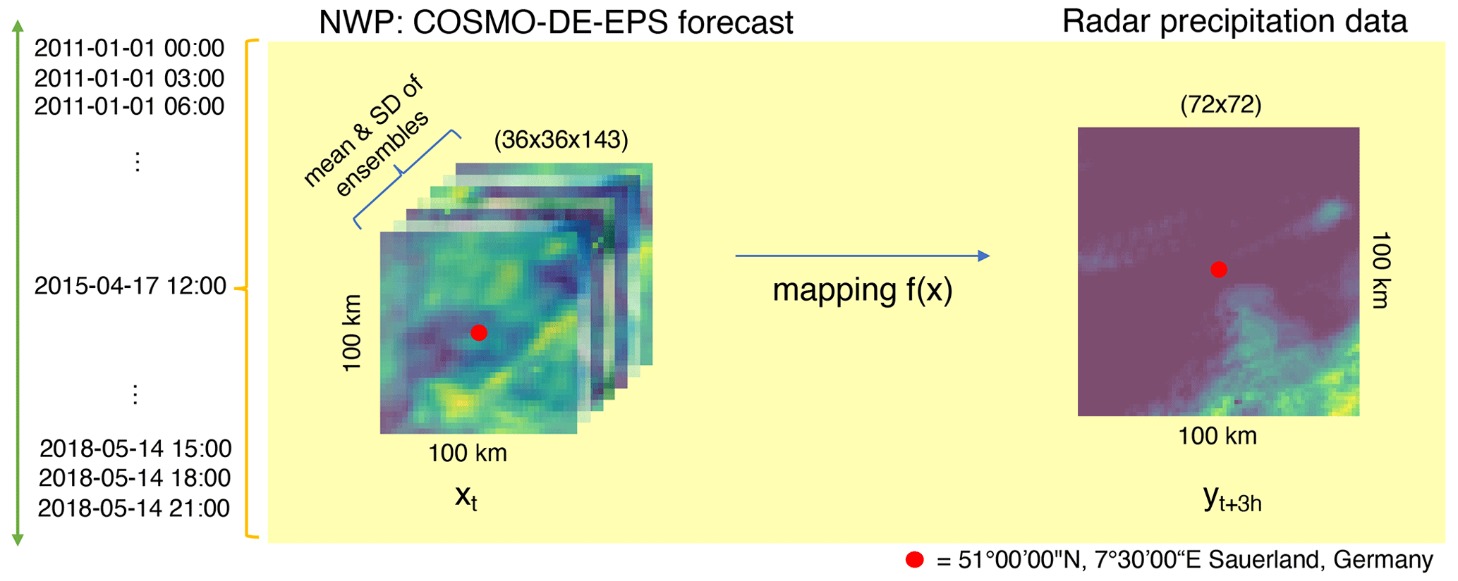
Figure 1 Task description: our research goal is to perform a direct mapping between the low-resolution atmospheric forecast and the high-resolution radar observations using the complete information of the NWP as input.

In this matter, we propose a new and alternative solution: to use the complete low-resolution weather simulations (NWP) as an informed prior for training a system that produces high-resolution precipitation maps. This translates into using deep learning algorithms to directly map the low-resolution meteorological forecast with high-resolution radar observations, generating short-term (3 h) and high-resolution (1.4 km) precipitation maps based on the nonlinear combination of all variables of the numerical weather simulations (NWP), correcting forecast inaccuracies in the process (see Fig. 1).

Our research goal is to achieve this mapping by developing and testing different deep learning algorithms in their ability to generate precipitation maps while increasing the resolution of the output. We will start by describing the data we worked on: the COSMO-DE-EPS simulations as input and precipitation radar images as output. Later, we present the different algorithms we trained and tested, their implementation and optimization procedures, and the metrics used to evaluate the generated predictions. The results obtained by each model are examined using the current literature.

2 Data

The complete dataset was composed of all eight initializations of the COSMO-DE-EPS forecast with 3 h lead time and their target precipitation radar observations over the period between the beginning of 2011 until the end of May 2018, in a selected area of about 100×100 km² in the region of West Germany (see Fig. 2).

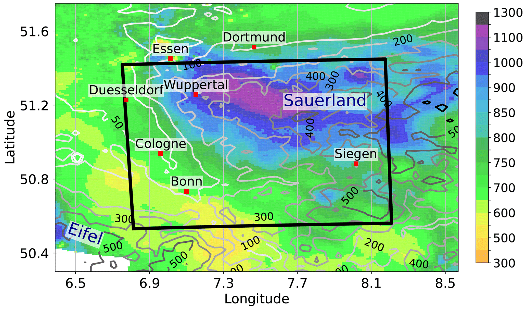
Figure 2 Average yearly precipitation (colors, mm yr⁻¹) from 2001–2021 compiled from the RW product (rain-gauge-adjusted hourly precipitation) of the RADKLIM dataset (see Sect. 2.2). The lateral boundary of the target region is highlighted by the black box. Contour lines show the surface elevation retrieved from the SRTM dataset (NASA JPL, 2013).

The selected area is located in the central parts of West Germany where interaction between low mountain ranges and the dominant flow patterns induces strong spatial variability in the yearly precipitation amount (see also, e.g., Kreklow et al., 2020). Due to prevailing westerly and southwesterly winds, the southwestern part of the target area is characterized by low precipitation amounts between 500 and 700 mm yr⁻¹ due to lee effects of the Eifel mountain range. By contrast, yearly precipitation exceeds 1200 mm yr⁻¹ between Wuppertal and Luedenscheid due to lee effects at the Sauerland mountain range. The high spatial variability in precipitation together with a good data coverage due to the overlapping observation area of different radar stations (see Fig. 1 in Pejcic et al., 2020) make the region suitable for testing our deep neural networks.

2.1 NWP output

We use the output of the COSMO-DE-EPS forecast (Peralta et al., 2012) as input; this was known as the German Meteorological Service (DWD) operational ensemble predictions system until May 2018, providing numerous data points for developing and testing deep learning applications. The COSMO-DE-EPS is the German adaptation of the COSMO model, a well documented and reliable NWP model operating in several EU countries (Marsigli et al., 2005; Valeria and Massimo, 2021).

We selected the forecast with 3 h of lead time. We calculate the mean and standard deviation (i.e., ensemble spread) from the 20 ensemble members for a total of 143 forecasts. Each of the forecast variables provided information about meteorological states (wind speed, temperature, pressure, etc.) and soil and surface states (water vapor on the surface, snow amount, etc.), providing a multidimensional description of the atmospherical state for the time predicted. A detailed description of the COSMO-DE-EPS output can be consulted in Schättler et al. (2019).

Given that each pixel of the COSMO-DE-EPS grid covered 7.8 km² (2.8×2.8 km), the correspondent 100 km² forecast around the coordinates (51^∘00^′00^′′ N, 7^∘30^′00^′′ E​​​​​​​) has an extension of 36×36 pixels and we have 143 variables (channels); this give a final shape of $\mathrm{36}\times \mathrm{36}\times \mathrm{143}$ forecast for the area.

2.2 Radar precipitation observations

Our prediction target constitutes quality controlled precipitation observations of the German radar network provided by the DWD. Here, we use version 2017.002 of the RADar KLIMatologie (RADKLIM – radar climatology) dataset (Winterrath et al., 2018). This dataset is based on the RADar OnLine AdjustemeNt (RADOLAN) procedure which converts the reflectivity measured by 17 ground-based C-band radar stations to precipitation rates (Bartels et al., 2004). The procedure constitutes a synthesis between radar and rain gauge observations and includes several corrections to eliminate backscattered noise due to non-meteorological targets (e.g., insects or solid objects like wind power plants). Additional corrections are included for the RADKLIM dataset compared to the RADOLAN procedure (Winterrath et al., 2018).

The radar data are given on a polar stereographic grid which provides a quasi-equidistant grid coverage over Germany at a resolution of 1 km. For consistency between the input and the target, the Climate Data Operators (CDO) software (Schulzweida, 2019) is used to remap the data onto the same rotated pole grid as the COSMO data (see Sect. 2.1), but at a higher spatial resolution of 1.4 km for downscaling purposes. The first-order conservative remapping method provided by the YAC (Yet Another Coupler) interpolation stack (Hanke et al., 2016) ensures that the area-integrated precipitation amount is approximately conserved during the remapping process. Additionally, the YW product which provides precipitation rates for every 5 min is used to retrieve hourly precipitation. This is mandatory, since the original hourly RQ product is not valid at full hours but at minute 50, which would in turn result in a mismatch with the time stamp of the NWP data. The resulting target data then comprise 72×72 pixels which are aligned with the coarser NWP input data.

3 Methodology

According to the recent literature, two main deep learning approaches can be considered helpful to solve this task: deconvolution models and conditional generative adversarial models. Both of these approaches perform a nonlinear mixing of the input variables to generate high-resolution precipitation maps.

Deconvolution models use deconvolution layers to increase the resolution of the input. The deconvolution operation (also called transposed convolution or unsampled convolution) works inversely to convolution. Instead of creating an abstract representation of the input by reducing its spatial dimension, deconvolution upsamples the input to the desired feature map using learnable parameters by multiplying it by a kernel (Dumoulin and Visin, 2018). Deconvolution techniques have been widely used in super-resolution (Long et al., 2015) and image-segmentation tasks (Ronneberger et al., 2015). However, applications of deconvolution networks to generate precipitation maps (Ayzel et al., 2020) have generated blurry outputs with high spatial smoothing, making the images look unrealistic and fail to predict high precipitation events.

On the other hand, generative adversarial networks (GANS) have been used to generate realistic precipitation maps that do not incur spatial smoothing or blurring (Ravuri et al., 2021). Generative adversarial networks are a generative model composed of two separate networks: a generator network that creates a fake image from a random input and a discriminator network, with the job of discriminating between the real and the fake images. While the generator is trained to try to deceive the discriminator, the discriminator is trained to separate the authentic images from the fake ones. Both networks are trained against each other, which forces the generator to create realistic outputs (Goodfellow et al., 2014).

Generative adversarial networks can also be used to solve image-to-image translation tasks by substituting the random input for a conditional input (Isola et al., 2016) (now called conditional generative adversarial networks or CGANs). While the task of the discriminator remains unchanged, the generator is asked to not only fool the discriminator but also be near the truth value, combining the loss with the distance between output and true values regulated by a hyperparameter lambda. In this way, the generator produces an output that is not only accurate but also resembles the characteristics of a real image.

Table 1 Summary of the deep learning models trained and tested in this study.

In this work, five different deep learning models were developed and tested: two baseline models for comparison with previously published algorithms, two deconvolution models and the CGAN. The development of the deconvolution models and the CGAN were guided by previously published literature about deep learning applications for super-resolution tasks but adapted to our dataset characteristics and the results of hyperparameter experimentation. Validation of hyperparameters and parameters is performed by testing the model against unobserved data (test set). Each of the models is explained in detail next and summarized in Table 1.

3.1 Deep learning models

3.1.1 Baseline model

As a baseline comparison point, a single 7×7 deconvolution kernel with a ReLU (rectified liner unit) activation function is used to generate a single precipitation map. The kernel combined the local input information to calculate a high-resolution rain map. The goal of this model was to offer a baseline comparison point of the simplest model to compare with more complex models.

3.1.2 U-Net

As mentioned in the introduction, the U-Net architecture (Ronneberger et al., 2015) was previously used to nowcast and downcast meteorological data. The U-Net is composed of an initial contracting path followed by an expansive path that increases the resolution of the output, adding skip connections between the stages of the paths.

Due to its proven good performance in the abovementioned tasks, it was considered essential to explore its performance in solving our present task and have it as a reference point to evaluate the performance of our models. In this work, we adapt the architecture used by Ayzel et al. (2020) to the dimensionality of our input and output data while conserving the essential contracting and expanding paths. The detailed architecture can be found in Appendix A.

3.1.3 One-level deconvolution (Deconv1L v1)

In the Deconv1L, a first 7×7 deconvolution kernel is applied to the input that generates 32 high-resolution feature maps. Next, batch normalization is applied to avoid overfitting, followed by a convolution kernel that combines the 32 feature maps into a single precipitation image as output.

3.1.4 Three-level deconvolution (Deconv3L v1)

The Deconv3L model first applies max pooling to the input information to reduce its resolution to half (4.8 km²). After that, it applies a first deconvolution 5×5 kernel to generate 32 feature maps, followed by batch normalization. An additional deconvolution kernel is applied over the generated feature maps to generate 16 combined feature maps. Finally, a single convolutional kernel estimates the output layer based on the previously mixed maps.

3.1.5 Conditional adversarial generative networks (CGAN v1)

For the CGAN, the Deconv3L was used as a generator to create rain maps based on the COSMO-DE-EPS input. Additionally, a discriminator model was implemented with the task of distinguishing between authentic images and generated images. The discriminator network was composed by three blocks of a convolution kernel together with a dropout layer, followed by a flattening of the feature maps and a fully connected output. Different from the previous models, the difference between the generated images and the actual values was not directly back-propagated to the weights. Instead, the generator loss is a combination of the distance between the predictions and outputs with an attempt to fool the discriminator, which leads the generator to create realistic outputs based on the input without blur.

3.2 Implementation

The training of the models was performed on the JUWELS Supercomputer at the Jülich Supercomputing Centre (JSC), on standard compute nodes. Each node contained 2 Intel Xeon Platinum 8168 CPU with 24 cores each of 2.7 GHz, and 96 GB DDR4 of ram at 2666 MHz. The training took between 30 min and 1 h, depending on the complexity of the model. The implementation was based on Python 3.8.3 (Van Rossum and Drake, 1995). Array operations were performed using Numpy 1.19.1 (Harris et al., 2020) and TensorFlow 2.3.1 (Abadi et al., 2015) was utilized to implement the deep learning algorithms together with the Keras 2.4.0 library (Chollet et al., 2015). The mpi4py 3.0.3 library (Dalcin et al., 2019) was used to distribute the initializations training on different JUWELS JSC cores. Scikit-Learn metrics 0.23.2 (Pedregosa et al., 2011) were used for verification and Matplotlib (Hunter, 2007) for plotting the results.

The complete implementation was subdivided into three sections. First, preprocessing was needed to prepare the data for training and to generate the different datasets from the complete set of forecasts and observations. Given that the performance of deep learning models can be affected by the random initialization of the kernel parameters, 20 independent random initializations were trained for each of the models of interest to make the study's results robust. Thereafter, each model initialization was trained using the training set and monitored using the validation set. Lastly, the performance of each model initialization was evaluated using the test set. Each of the steps is explained in detail in the following subsections.

3.2.1 Preprocessing

The first step of the preprocessing was to match each of the COSMO-DE-EPS forecasts with their corresponding radar observation. All forecast–precipitation pairs containing any missing values were discarded (3.93 % of the total). Next, the original values of the forecast were standardized in order to avoid numerical problems due to inputs in different units of measurement. The complete dataset was split into train, test and validation set by date. All forecasts with dates of 1st, 9th, 17th and 25th, regardless of month and year, were selected as part of the test set (2671 forecasts and observations, 12.96 % of the samples). In the same way, the validation set was built with the forecast of the 5th, 13th, 21st and 28th of all months and years (2725 forecast and observations, 13.25 % of the complete set). Then, all remaining dates were chosen as part of the training set (15 189 forecast and observations, 73.79 % of the dataset). Finally, the three datasets were stored and retrieved using the TFRecords format from the TensorFlow library (Abadi et al., 2015) (the complete preprocessing routine was implemented and can be found in the notebook preprocessing.ipynb, part of the repository part of this paper).

3.2.2 Training

One single script was developed (baseline.py, unet.py, deconv1l.py, deconv3l.py, and cgan.py) for each model. The 20 initializations of each model were distributed between 20 independent cores of the JSC HPC in the mpi4py library (Dalcin et al., 2019). Each core reads the training set stored as TFRecords, initializes a model with random initial weights and fits the parameters to the training set. The training was performed during 24 epochs using a mini-batch size of 20. Mean squared logarithmic error (MSLE) was used as the loss measure due to the gamma-like distribution of the rain amount on the radar images (see Fig. 3), and Adam, with a learning rate of 0.001, was used as the optimizer. Once each core finished its respective training, the resulting model was stored in TensorFlow HDF5 format, and their loss during training was saved and plotted to check for convergence.

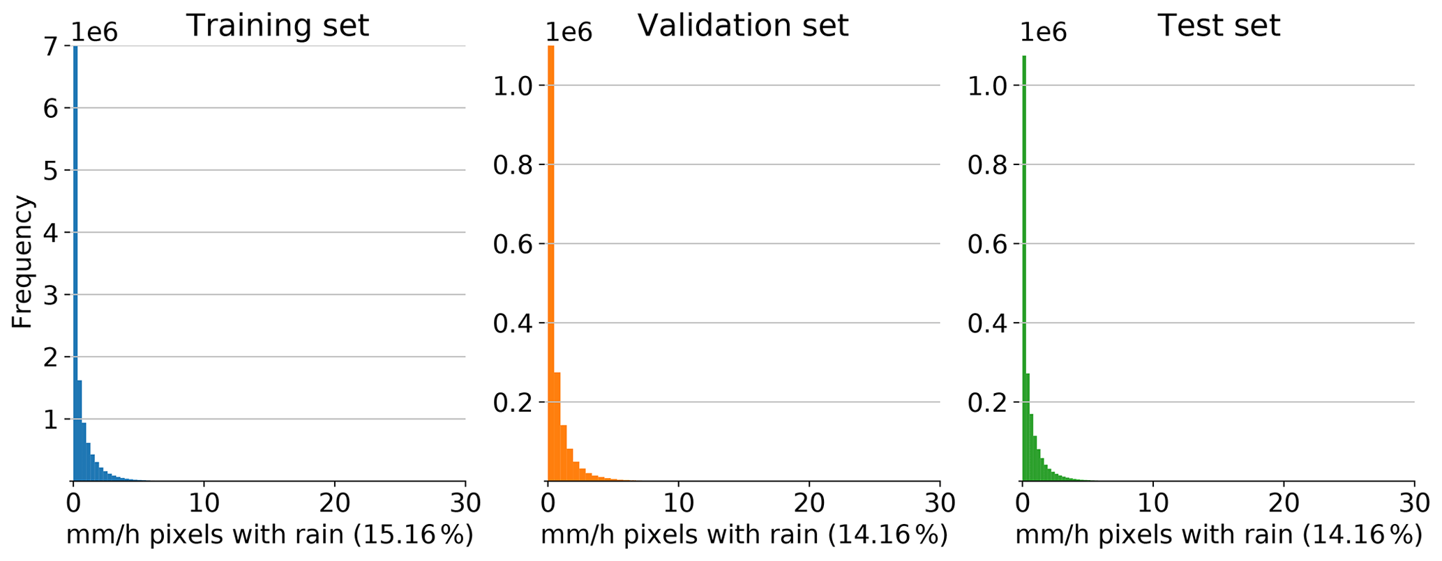
Figure 3 Distribution of registered precipitation for pixels with precipitation > 0 mm h⁻¹ in the radar observations. In all datasets, the majority of the pixels registered no rain. For the pixels with rain, we found the rain amounts to characteristic gamma-like distribution.

3.2.3 Verification and plotting

Once the trained models were stored, their performance was evaluated using the test set (evaluate.ipynb). Each of the 20 initializations was loaded and used to generate predictions for the input test set. Next, the predictions were evaluated using the verification methods (detailed in the following section) and the results were stored. Finally, the evaluations of each model were plotted and illustrated (plot.ipynb).

3.3 Verification methods

Predictions generated by the trained models, as well as the predictions from COSMO-DE-EPS, were evaluated using two different types of metrics: continuous and dichotomous. The continuous verification metrics were skill scores based on mean absolute error (MAE) and linear error in probability space (LEPS). The output of the models was also evaluated using three different dichotomous metrics based on the truth table – critical success index (CSI), equitable threat score (ETS) and frequency bias – for which five different thresholds were applied to the output: 0.2, 0.5, 1, 2 and 5 mm h⁻¹. Each of the verification metrics is presented in detail in the following paragraphs.

3.3.1 MAE-based skill score

The mean absolute error measures the absolute difference between paired observations expressing the same phenomenon, in this case, the difference between the forecast and the observed radar images. Considering F as the forecast vector and O as the observations, the MAE is defined as follows:

$$\begin{array}{}\text{(1)}& \mathrm{MAE}={\displaystyle \frac{\mathrm{1}}{N}}\sum _{i=\mathrm{1}}^N|{\mathit{F}}_i-{\mathit{O}}_i|.\end{array}$$

The term “skill score” indicates the degree of improvement of the new predictions compared to the original COSMO-DE-EPS forecast. The forecast is perfect when the skill score equals 1, while a skill score of 0 and below indicates that there is no improvement or less skill in the new predictions compared to the reference. The MAE-based skill score is calculated as follows:

$$\begin{array}{}\text{(2)}& \mathrm{skill}\mathrm{score}=\mathrm{1}-{\displaystyle \frac{{\mathrm{MAE}}_{\mathrm{model}\mathrm{predictions}}}{{\mathrm{MAE}}_{\text{COSMO-DE-EPS predictions}}}}.\end{array}$$

3.3.2 LEPS-based skill score

The linear error in probability space is the mean absolute difference between the values that the forecast and observation take in the climatological cumulative distribution function (CDF) of the observations, i.e., LEPS is analogous to the MAE but in a CDF space (Ward and Folland, 1991). Considering F as a distinct forecast, O as the respective observation and CDF_o as the CDF of the observations determined by an appropriate climatology, LEPS is defined as follows:

$$\begin{array}{}\text{(3)}& \mathrm{LEPS}={\displaystyle \frac{\mathrm{1}}{N}}\sum _{i=\mathrm{1}}^N\left|{\mathrm{CDF}}_{\mathrm{o}}\right({\mathit{F}}_i)-{\mathrm{CDF}}_{\mathrm{o}}({\mathit{O}}_i\left)\right|.\end{array}$$

Similar to other skill scores, a perfect forecast obtains a skill score equal to 1 and a skill score of 0 and below would indicate a decrease in the performance compared to the reference models. The LEPS-based skill score is calculated as follows:

$$\begin{array}{}\text{(4)}& \mathrm{skill}\mathrm{score}=\mathrm{1}-{\displaystyle \frac{{\mathrm{LEPS}}_{\mathrm{model}\mathrm{predictions}}}{{\mathrm{LEPS}}_{\text{COSMO-DE-EPS predictions}}}}.\end{array}$$

3.3.3 Equitable threat score (ETS)

The ETS measures the skill of the forecast relative to chance by measuring the fraction of the observed forecast events that were correctly predicted, adjusted for corrected predictions associated with random chance. It ranges between $-\mathrm{1}/\mathrm{3}$ and 1, with 0 and below indicating no skill and 1 representing a perfect forecast. Specifically, it is calculated in the following way:

$$\begin{array}{}\text{(5)}& \mathrm{ETS}={\displaystyle \frac{\mathrm{hits}-{\mathrm{hits}}_{\mathrm{random}}}{\mathrm{hits}+\mathrm{misses}+\mathrm{false}\mathrm{alarms}-{\mathrm{hits}}_{\mathrm{random}}}},\end{array}$$

where

$$\begin{array}{}\text{(6)}& {\mathrm{hits}}_{\mathrm{random}}={\displaystyle \frac{(\mathrm{hits}+\mathrm{misses})(\mathrm{hits}+\mathrm{false}\mathrm{alarms})}{\mathrm{total}}}.\end{array}$$

3.3.4 Critical success index (CSI)

The CSI measures the fraction of observed and/or forecast events that were correctly predicted. It ranges between 0 and 1, with 0 indicating no skill and 1 representing a perfect score:

$$\begin{array}{}\text{(7)}& \mathrm{CSI}={\displaystyle \frac{\mathrm{hits}}{\mathrm{hits}+\mathrm{false}\mathrm{alarms}+\mathrm{misses}}}.\end{array}$$

3.3.5 Frequency bias (BIAS)

The frequency bias measures the ratio of the frequency of forecast events to the frequency of observed events. It indicates whether the forecast has a tendency to under-forecast (BIAS < 1) or over-forecast (BIAS > 1). It ranges from 0 to ∞ with a perfect score of 1 and does not measure how well the forecast corresponds to the observations, only relative frequencies:

$$\begin{array}{}\text{(8)}& \mathrm{BIAS}={\displaystyle \frac{\mathrm{hits}+\mathrm{false}\mathrm{alarms}}{\mathrm{hits}+\mathrm{misses}}}.\end{array}$$

4 Results

Our research goal was to explore the application of deep learning models to generate high-resolution precipitation maps using low-resolution NWP simulations as input. We developed and tested five deep learning algorithms to achieve this goal. For each model, 20 independent runs with initial randomization were performed, and their predictions were evaluated using the aforementioned metrics.

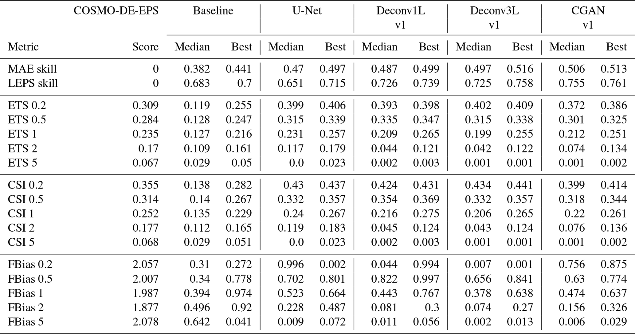
Table 2 Summary of the results: median and best-performing model are presented for each of the metrics.

Perfect score for all metrics =1.

The results of this work demonstrate the general ability of deep learning algorithms to calculate high-resolution precipitation maps. As in most machine learning applications, a significant influence of the architecture and the total number of parameters was found; this suggests that the algorithm's ability to solve these tasks depends on finding the right level of complexity for the problem. The scores are summarized in Table 2 and illustrated in Figs. 4 and 5. The models' predictions are shown in Fig. 6. A detailed analysis of the performance of each model is presented next.

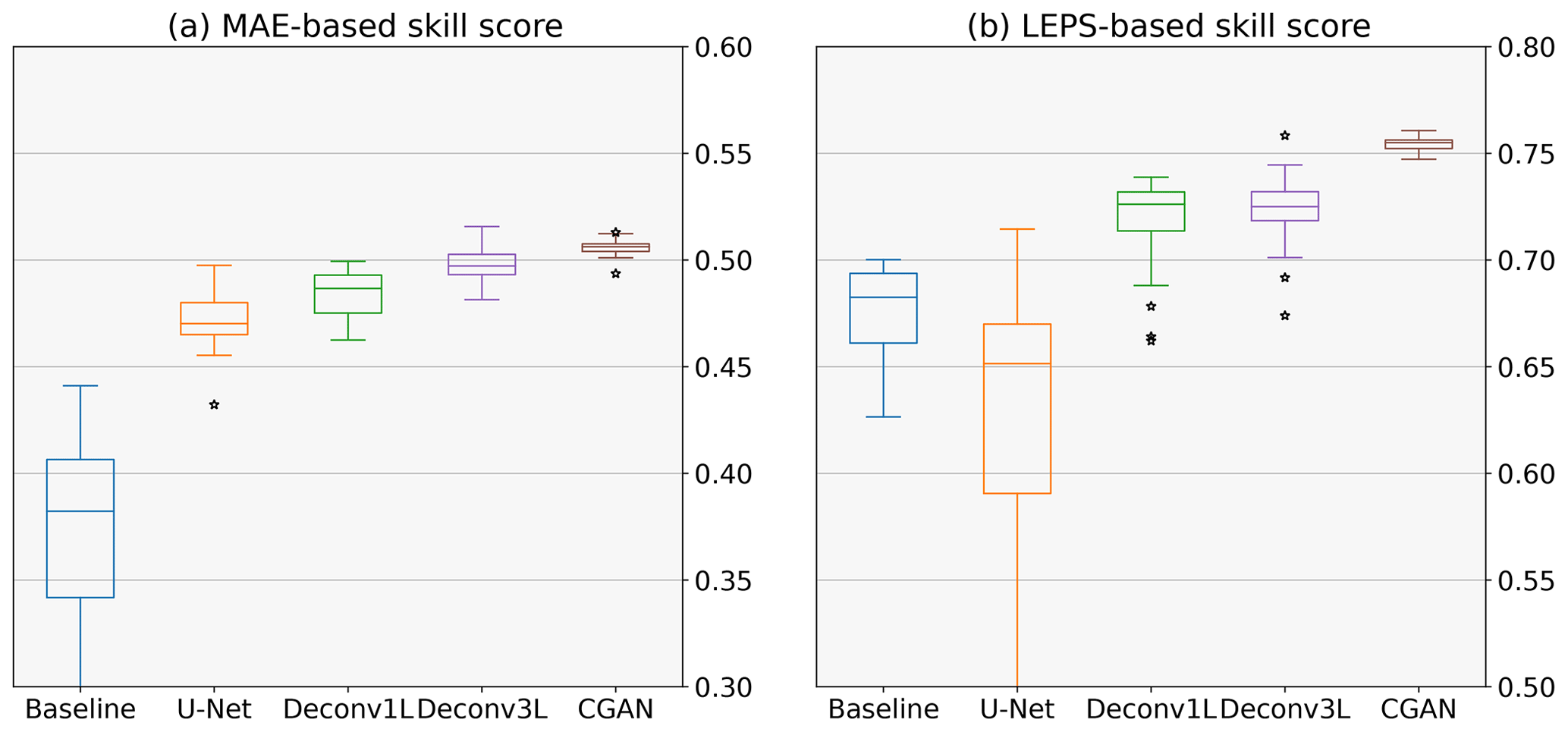
Figure 4 Quantitative metrics: each subplot compares the skill score of the different models. In panel (a), each boxplot illustrates the MAE-based skill score, and in panel (b), the LEPS-based skill score of 20 runs for each model with different initializations is depicted. The higher the skill score, the higher the improvement over the reference (in this case, COSMO-DE-EPS). A skill score of 0 represents no improvement, and a negative skill score indicates decay in the performance.

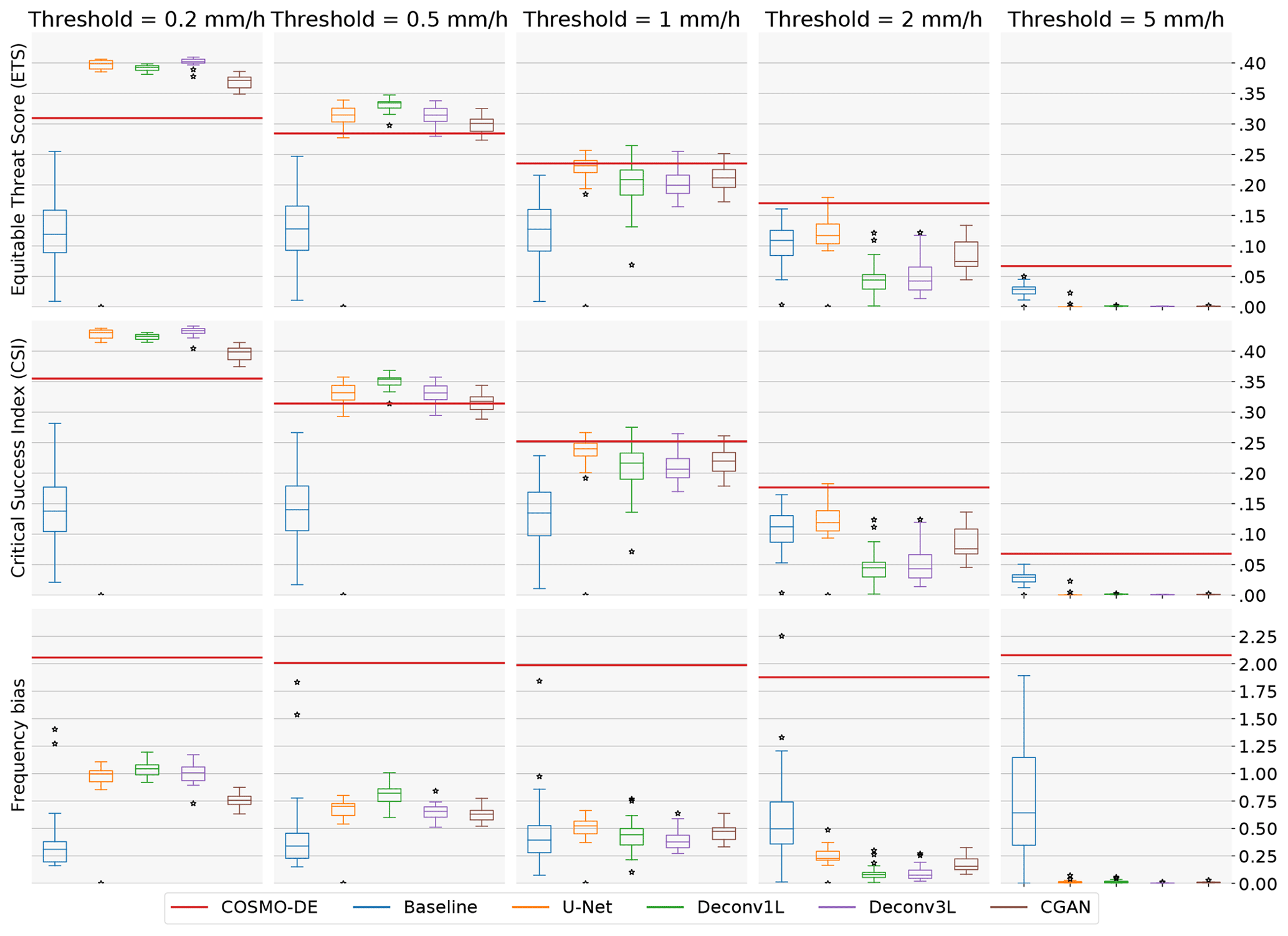
Figure 5 Dichotomous metrics: each subplot illustrates the metrics score of 20 independent models with different initial conditions after a certain threshold was applied. The ETS and CSI vary between 0 and 1, with 0 indicating no skill and 1 a perfect forecast. Frequency bias ranges from 0 to +∞, with bias < 1 indicating under-forecasting, bias > 1 indicating over-forecasting and a perfect score =1.

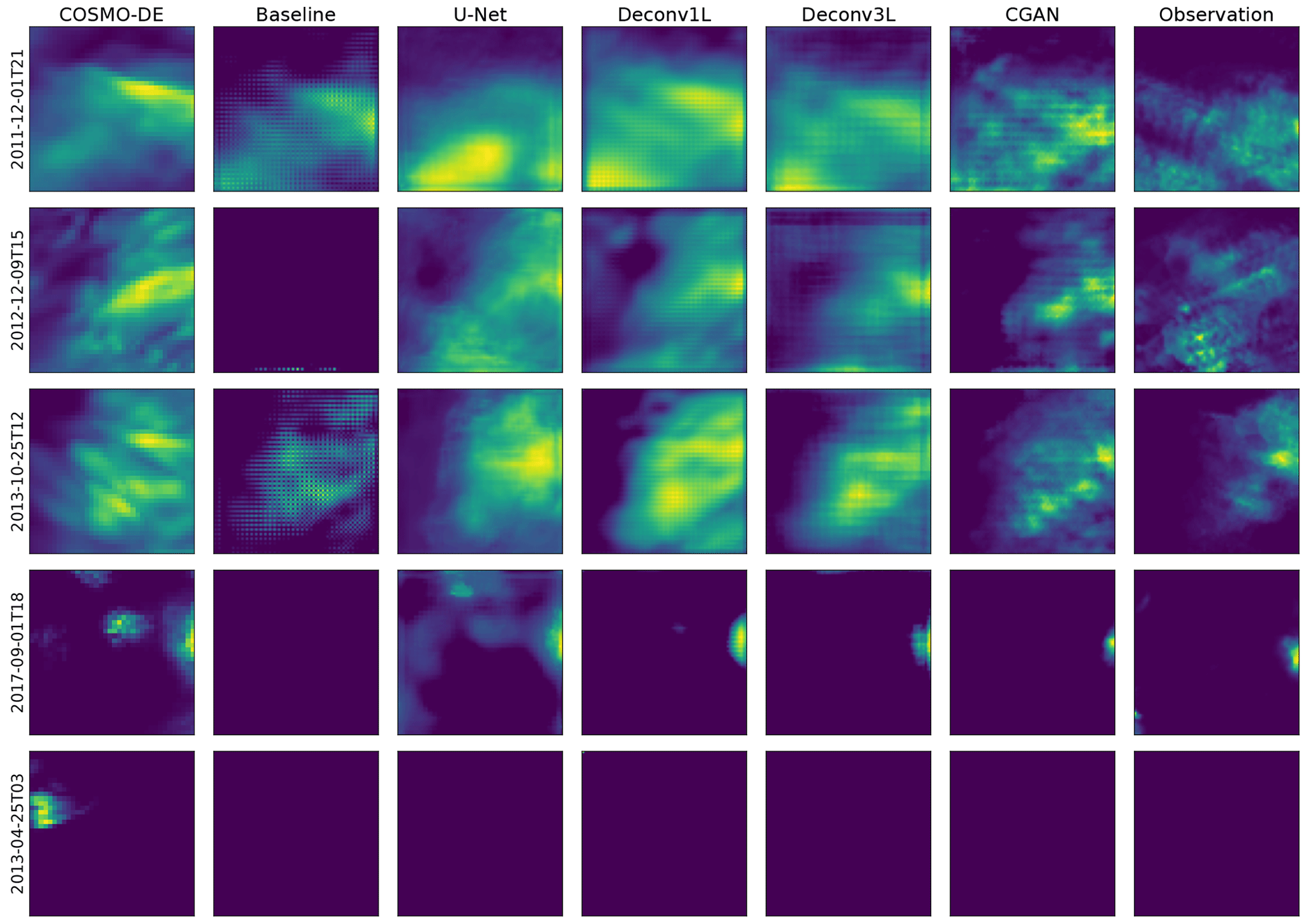
Figure 6 Example of predictions made by the different models versus the true values. For each of the models, the initialization with the highest LEPS-based skill score was selected to generate the predictions.

First, we need to evaluate the skill of the original COSMO-DE-EPS to forecast precipitation. To do so, we compared the total precipitation variable against a low-resolution version of the radar observation using all metrics. To merge the RADKLIM data onto the rotated pole grid of the COSMO-DE-EPS data, a conservative remapping step with CDO is performed, similar to the procedure described in the “Data availability” section.

Given that MAE- and LEPS-based skill scores are calculated in reference to the COSMO-DE-EPS performance, the respective skill scores are equal to 0. Following the ETS and CSI scores, we observe an initial high performance of the model in low-threshold events and a progressive decline with the threshold increase. This finding indicates a good general skill to predict low rain events and less skill to predict high precipitation events. However, COSMO-DE-EPS presents the highest scores in predicting high precipitation events (2 and 5 mm h⁻¹). Analyzing the frequency bias, a strong tendency to over-forecast rain regardless of the thresholds can be observed, a tendency that can be confirmed by examining the example predictions in Fig. 6.

Starting with the baseline model, we can observe an increase in both skill scores concerning COSMO-DE-EPS. This improvement is limited compared to more complex models, which is expected due to the simplicity of the model and the reduced amount of parameters involved. Regarding ETS and CSI, a significant decrease in the median scores in all thresholds can be viewed, together with high variability, which signalizes a lack of consistency in the models' performance. Observing the example precipitation maps, the problem comes to light: the precipitation maps show checkerboard artifacts which lead to numerous rain points being missing. This artifact is caused by the superposition of the kernel operation caused by the only deconvolution layer included in the model. Despite the artifacts, the model generates a significant improvement in the frequency bias, obtaining values close to 1 in small thresholds. However, these results disappear at higher thresholds, indicating that the model does not produce stable results.

The second comparison point was the U-Net-based model. The U-Net model presents a significant improvement in absolute error but a decrease with very high variability in the LEPS-based skill score. By observing the ETS, CSI and frequency bias scores, a substantial improvement can be observed in its ability to predict low rain events. Regarding the performance for thresholds of 1 and 2 mm h⁻¹, this architecture obtains even better median scores than the more complex models, indicating a good ability to predict mid-range rain events. These scores suggest that the U-Net model has a lower bias towards rain amounts of 0 than the baseline model and is prone to generating medium rain forecasts, which generates a higher average error that is reflected by the high variability of the LEPS-based skill score. This effect can be confirmed in the precipitation maps with more extensive and more intense precipitation regions.

Moving to the main models of this work, the first deconvolution model, Deconv1L, significantly outperforms the baseline and U-Net models in the MAE- and LEPS-based skill scores. Observing the ETS and CSI scores, we can see a significant improvement in predicting low rain events, obtaining the best scores between all models for 0.5 and 1 mm h⁻¹ thresholds. However, this ability starts to decrease significantly with the utilization of higher thresholds, which indicates the presence of a bias from the model to favor low precipitation events and difficulties in predicting high rain events. This tendency can be confirmed by observing the frequency bias, where the Deconv1L model obtains almost perfect scores for low thresholds but under-forecasts for rain events of higher intensity. The example rain maps confirmed a solid tendency to predict low rain events when generating spatial smoothing of the rain maps, which also explains the increase in the skill scores.

In the case of Deconv3L, we found a similar but slightly better performance compared to Deconv1L for the quantitative metrics. The median MAE-based skill score is above all previous models, and the median LEPS-based skill score is comparable to the Deconv1L, with the best initialization outperforming all previous models. Looking at the ETS and CSI, we found a similar performance to the Deconv1L model, with minor improvements in the 0.2 mm h⁻¹ threshold but a slight decrease in the performance of all other thresholds; this indicates a higher bias to perform spatial smoothing and to favor low rain events. This bias can be confirmed by observing the frequency bias scores, where the performance improves for the small thresholds but then decays compared to Deconv1L in all other thresholds. Example predictions confirm similar spatial smoothing found in other deconvolution models. However, it is essential to consider that this model reaches comparable performance to Deconv1L using approximately half of the parameters, enabling more efficient use of computational resources.

Considering the superior performance shown by the Deconv3L model, we used it as a generator model in a conditional generative adversarial model (CGAN). A significant improvement in performance and consistency can be found using Deconv3L as a generator in the MAE- and LEPS-based skill scores. For lower thresholds (0.2 and 0.5 mm h⁻¹), we observe a decay in the performance compared to the deconvolution models but improved scores for higher thresholds. Additionally, the CGAN models have a lower frequency bias for these same thresholds. These metrics indicate a better model performance to predict high precipitation events, indicating a correction of the spatial smoothing caused by the deconvolution operation. This correction is confirmed by observing the prediction examples, where we can find the more realistic high-resolution outputs between all models.

In summary, COSMO-DE-EPS tends to overpredict rain events shown by a high-frequency bias and poor scores in ETS and CSI for lower thresholds. This tendency can be partially corrected by implementing deconvolution models that present a superior performance to the reference models (baseline, U-Net). However, these deconvolution models induce a new type of bias towards low rain events which provoke spatial smoothing in the examples and reduces the total level of error; it also increases the accuracy for low rain events while deteriorating the skill to predict high precipitation events. This blurry effect can be countered by integrating the deconvolution model as a generator in a conditional generative model which can generate accurate outputs resembling real rain maps. An additional finding was that the U-Net architecture did not achieve superior or stable scores for this problem. Possible reasons for this are discussed in the following section. Additionally, all models present a decrease in the scores when increasing the rain thresholds, indicating a general difficulty in predicting high precipitation events.

5 Conclusions

The results obtained in this work provide significant evidence for the application of deep learning models to perform bias correction of the NWP input and to generate high-resolution rain maps with improved accuracy. This improvement proves that using the complete information of the NWP variables and combining them in a nonlinear fashion using feature maps helps to achieve higher quality and more precise precipitation forecasts.

The direct mapping between the physical simulations of the weather and the precipitation maps captured by radars can be achieved with the use of deep learning algorithms in a single step that combines increasing the resolution and correcting such inaccuracies of the original forecast. A significant amount of improvement performed by the deep learning models consisted of correcting the tendency of the COSMO-DE-EPS to over-forecast, but the application of the developed models introduced new different types of bias.

The U-Net-based model presented an important bias to mid-range precipitation, which increased the average error of the predictions and made it less suitable to solve the task. A possible reason is that the contracting path of the architecture destroyed a significant part of the needed information to generate high-resolution predictions, causing the network to overestimate the amount of rain registered and, therefore produce inaccurate predictions.

This conclusion is sustained by the observation that the architecture of one of the best-performing models (Deconv3L) is inspired by the U-Net architecture, except for the contracting path that is substituted with a single max-pooling layer. The performance and consistency shown by the Deconv3L model are highly superior to the U-Net network. This is in contrast with a series of works in the last years that used the U-Net architecture for super-resolution tasks with meteorological data (Ayzel et al., 2020; Serifi et al., 2021). In this particular case, where the input has an elevated number of channels (in this case, 143), the expanding path alone provided higher performance than the complete U-shaped structure.

On the other hand, the spatial smoothing caused by the deconvolution operation that has been reported in previous works (Ayzel et al., 2020; Ravuri et al., 2021) was also reproduced by our deconvolution models. Consistent with the work of Ravuri et al. (2021), using the Deconv3L model as a generator in a conditional generative model helped to find the right trade-off between accuracy and realistic outputs and generated realistic high-resolution rain maps with the lowest error between all models. This gain in performance is due to back-propagating a combined loss function (chances to fool the discriminator and distance to real values) instead of only the difference between the real values and the model predictions, which avoids the fact that the model only optimizes in terms of the mean squared logarithmic error, causing the spatial smoothing.

An additional conclusion from this work is the relevance of using multiple metrics for the evaluation of precipitation predictions. Our results showed that the utilization of the LEPS could reveal inconsistencies first unattended by the MAE. Especially in the case of precipitation, the single use of MAE as a performance metric can be misleading due to the values' closeness to 0.

We provided important information about the characteristics of the application of models with different characteristics to the mapping between meteorological simulations and high-resolution rain maps that could guide the development of potential real-world implementations. The first limitation of our results is the limited spatial and temporal resolution of our predictions. Our scope was limited to a forecast lead time of 3 h and an area of 100×100 km², which is a small domain when compared to real meteorological applications. Also, nowcasting applications usually provide predictions for several time points in the future while our work is limited to one. Additionally, modern practical meteorological applications offer probabilistic outputs, and our models generate deterministic predictions which would be a limitation for a direct application of the algorithms. Most of these limitations are caused by our intention to generate an initial approximation of the capabilities of deep learning to solve this task instead of generating a fully functional and applicable model.

The key element for the improvement of the quality of the forecast is the inclusion of multiple variables (as channels) which provide enough information about the different states of the atmosphere and soil. The developed models combine and weights the input information (and its combinations), learning the relevant patterns in the input information to correct the precipitation predictions and increase its resolution. Nonetheless, combining multiple variables entails two consequences: first, it requires higher computational resources to train the models than single or fewer variables. Second, it makes it very difficult to distinguish which variables are relevant to improve the forecast, given the nonlinear mixing performed by the algorithm. Future research must explore the relevance of single variables and train models with subsets of variables that make more efficient use of the computational resources.

Another shortcoming of our approach is overlooking the different types of precipitation. Our models make no explicit differentiation between the different types of rain (stratiform/convective). However, it could be that the best-performing models have learned different patterns of input information to improve each type of phenomenon, but proving this requires a different analysis that is out of the scope of the present work. Future research could explore generating distinct models for the different types of precipitation and the role of the different input variables for each type of precipitation.

The accurate prediction of high rain events remains a challenge, which is partially due to the limited number of samples to train the algorithms, making this an extremely difficult event to predict from the deep learning perspective. The integration of deep learning in meteorological workflows seems to be a useful tool for improving meteorological models. In our case, the use of deconvolution networks as a part of a CGAN provides promising results for the generation of accurate high-resolution precipitation outputs. Future research should extend the application of these models to bigger spatial and temporal domains, as well as more complex topographies, and at the same time, search for the set of hyperparameters that allows for decreasing inaccuracies in the predictions.

Appendix A: U-Net architecture

Table A1 Following the architecture proposed by Ronneberger et al. (2015) and Ayzel et al. (2020), the U-Net architecture was adapted to the input and output size of the current task using the following architecture.

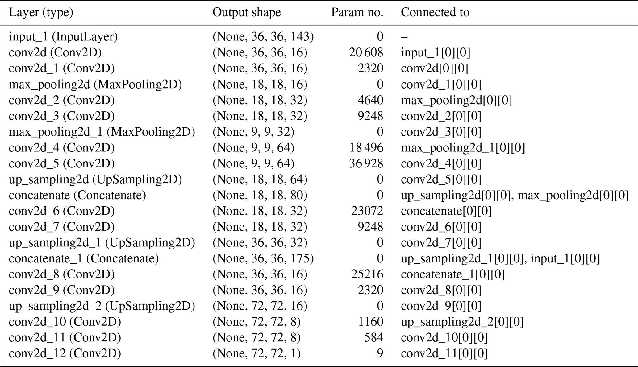
Total parameters: 153 849, trainable parameters: 153 849, non-trainable parameters: 0.