Sensitivity of NEMO4.0-SI³ model parameters on sea ice budgets in the Southern Ocean

The seasonally dependent Antarctic sea ice concentration (SIC) budget is well observed and synthesizes many important air–sea–ice interaction processes. However, it is rarely well simulated in Earth system models, and means to tune the former are not well understood. In this study, we investigate the sensitivity of 18 key NEMO4.0-SI³ (Nucleus for European Modelling of the Ocean coupled with the Sea Ice Modelling Integrated Initiative) model parameters on modelled SIC and sea ice volume (SIV) budgets in the Southern Ocean based on a total of 449 model runs and two global sensitivity analysis methods. We found that the simulated SIC and SIV budgets are sensitive to ice strength, the thermal conductivity of snow, the number of ice categories, two parameters related to lateral melting, ice–ocean drag coefficient and air–ice drag coefficient. An optimized ice–ocean drag coefficient and air–ice drag coefficient can reduce the root-mean-square error between simulated and observed SIC budgets by about 10 %. This implies that a more accurate calculation of ice velocity is the key to optimizing the SIC budget simulation, which is unlikely to be achieved perfectly by simply tuning the model parameters in the presence of biased atmospheric forcing. Nevertheless, 10 combinations of NEMO4.0-SI³ model parameters were recommended, as they could yield better sea ice extent and SIC budgets than when using the standard values.

1 Introduction

The Southern Ocean sea ice, a crucial component of the climate system, has experienced a slight but statistically significant expansion from 1979 to 2015 and remarkable fluctuations in the last few years (Comiso et al., 2017; Parkinson, 2019; Raphael and Handcock, 2022; Wang et al., 2022a). Several state-of-the-art climate models have successfully simulated the near-realistic annual cycle of sea ice area (SIA; Holmes et al., 2019), but they typically still fail to capture the observed sea ice variability and trends (Zunz et al., 2013; Turner et al., 2013; Shu et al., 2015, 2020). This implies that standard metrics commonly used for model evaluation, such as sea ice extent (SIE), SIA and total volume (SIV), are rather rudimentary and of limited use in improving the model skill (Notz, 2014, 2015), and better metrics are needed to optimize models.

Holland and Kwok (2012) proposed an analysis of sea ice concentration (SIC) budgets, i.e. decomposing the dynamic and the other processes leading to changes in SIC to compare with the same processes in observations, as an extension of the commonly used diagnostics for individual variables (e.g. SIC, ice thickness and ice drift). Diagnostics using SIC budgets for fully coupled climate models and ocean–sea ice models driven by atmospheric reanalysis showed that the relatively realistic sea ice extent in the models was the result of excessive sea ice velocity bias (Uotila et al., 2014; Lecomte et al., 2016). Correcting the sea ice velocity field in the model with satellite observations was able to simulate the trend of expanding sea ice extent in the Southern Ocean during 1992–2015 (Sun and Eisenman, 2021). Furthermore, correctly modelling the sea ice budget is so important, as the ocean can only be driven correctly if the sea ice budget is realistic (Holmes et al., 2019), which is related to the importance of sea ice in transporting fresh water (Abernathey et al., 2016; Haumann et al., 2016) and the role of sea ice as a mediator of polar air–ocean matter and energy exchange (Thomas and Dieckmann, 2010).

Sensitivity experiments with three different atmospheric reanalyses indicated that, at least in winter (April to October), SIC budgets are sensitive to atmospheric forcing, as sea ice models driven by these atmospheric reanalysis products show large errors compared to observations (Barthélemy et al., 2018). This was further validated by the fact that, even when using the same atmospheric reanalysis, the SIC budget in the ice–ocean reanalysis products can vary considerably (Nie et al., 2022). On the other hand, some studies have shown that simulations of the Southern Ocean sea ice area are not sensitive to model parameters (e.g. Massonnet et al., 2011; Uotila et al., 2012; Rae et al., 2014), but this is likely due to the dynamic and thermodynamic biases in the SIC budget cancelling out (Uotila et al., 2014), i.e. wrong processes lead to a right-looking result. Therefore, a hypothesis was proposed that model physics could be more important than previously recognized for improving sea ice modelling skills in the Southern Ocean (Barthélemy et al., 2018). Indeed, the conclusions of Uotila et al. (2014) showed that the SIC budget is sensitive to model configuration, and they surmised that it may be possible to adjust the model parameters to make the SIC budget components more realistic. An example is that, by changing the ice–ocean stress turning angle from 0 to 16^∘, the advection contribution to sea ice area change would be halved, although the divergence contribution would become unrealistic (Uotila et al., 2014). However, the sensitivity of the sea ice budgets to the model parameters has not been systematically assessed to date.

The most common approach for sensitivity experiments is to adjust a single variable of interest at a time while keeping all other parameters fixed (e.g. Fichefet and Morales Maqueda, 1997; Rae et al., 2014), but due to the complexity and strong non-linearity of the model, there are often interactions between variables that cannot be identified with this approach. Another approach is to adjust several variables simultaneously. Kim et al. (2006) tested the sensitivity of 22 parameters of the Los Alamos sea ice model (CICE) based on the automatic-differentiation method and adjusted the parameters to make the simulation as close as possible to the observations. Uotila et al. (2012) conducted experiments on 100 combinations of 10 parameters in a coupled ocean–ice model and recommended several optimal sets of parameters that would produce a realistic global sea ice distribution. To address the problem of the above sensitivity experiments being unable to fully explore the entire high-dimensional parameter space, a more attractive option is to do a global sensitivity analysis (GSA; Saltelli et al., 2008). However, a completely performed GSA requires a very large number of runs of the model – for example, O(10⁴) runs for O(10) parameters (Saltelli et al., 2010). One option is to build an emulator to quickly and with modest computational requirements predict the possible model outputs for a given input and as a substitute for the full dynamic model (Sacks et al., 1989; Kennedy and O'Hagan, 2000; Oakley and O'Hagan, 2004). In brief, an emulator is a machine learning method that statistically constructs relationships between inputs and outputs from existing model results.

There has been some success in quantifying the parameter uncertainty using emulators in ocean–sea ice models. For example, Urrego-Blanco et al. (2016) applied a Gaussian process (GP) emulator to perform the GSA on 39 parameters in CICE. Williamson et al. (2017) built an emulator for the NEMO ocean model and quantified the effect of uncertainty on the model for 24 parameters. In this paper, our research objective is to quantify the sensitivity of the Southern Ocean SIC and SIV budgets to key parameters in a coupled ocean–sea ice model by constructing a GP emulator and, furthermore, to verify whether the model parameters can be adjusted to obtain near-realistic SIC budget components. It is worth noting that NEMO4.0-SI³ parameters' default values are generally optimized based on Arctic observations (e.g. Warren et al., 1999; Perovich, 2002; Lüpkes et al., 2012), and here, we are investigating their optimal values from the perspective of the Southern Ocean SIC budget, which has not been done so far.

2 Materials and data

2.1 Model configuration and parameter space elicitation

Sea ice simulations in this study were performed using the version 4.0.7 revision 15 731 of the Nucleus for European Modelling of the Ocean (NEMO; NEMO System Team, 2022) coupled with the Sea Ice modelling Integrated Initiative (SI³; NEMO Sea Ice Working Group, 2019), hereafter called NEMO4.0-SI³. The model represents the global ocean via a commonly used nominal 2^∘ tri-polar grid (ORCA2), which has a resolution of about 85 km between 55 and 75^∘ S. The ORCA2 was chosen because it is already capable of identifying features of the Southern Ocean SIC budget at this resolution (Nie et al., 2022), and considering that hundreds of experiments will be performed, using ORCA2 is computationally comparably cheap. The ORCA2 grid configuration has 31 unevenly spaced vertical layers from 10 m thick (near surface) to 500 m thick (at 5500 m depth). The vertical physics of the ocean is solved by the combination of the turbulent kinetic energy (TKE) turbulent closure scheme (Marsaleix et al., 2008), an enhanced vertical diffusion scheme applied on tracer (Madec et al., 1998), and a double diffusive mixing scheme (Merryfield et al., 1999).

The sea ice momentum equation is calculated by using the adaptive elastic–viscous–plastic (EVP) method (Kimmritz et al., 2016, 2017), which is formulated on a C grid and improves the numerical efficiency of the modified EVP scheme. The default number of sea ice thickness categories is five, with each category having two vertical layers of ice and one layer of snow on top of ice. The thermodynamic component of NEMO4.0-SI³ includes the 1D energy-conserving model (Bitz and Lipscomb, 1999) and a time-dependent vertical salinity profile (Vancoppenolle et al., 2009). The sea ice model uses the same 1.5 h time step as the ocean model.

In this study, the NEMO4.0-SI³ model is forced with the DRAKKAR Forcing Set version 5.2 (DFS5.2; Dussin et al., 2016), based primarily on the ERA-Interim with some corrections (Dee et al., 2011) and covering the time period 1979–2017. The DFS5.2 provides the atmospheric field required for the NCAR bulk formula (Large and Yeager, 2004) in NEMO4.0-SI³, which includes 2 m air temperature, 2 m specific humidity, 10 m zonal and meridional wind speeds, mean sea level pressure, downward long-wave and short-wave radiation, and the total and solid precipitation rates. In these atmospheric fields, the frequency of radiation and precipitation is 1 d and 3 h for all other surface boundary conditions. The spatial resolution of DFS5.2 is approximately 80 km, close to that of ORCA2 in the Southern Ocean. The continental discharge rates followed the climatological dataset of Dai and Trenberth (2002) and do not include ice mass loss in Antarctica. The simulations are initialized at rest via the temperature and salinity fields from the World Ocean Atlas 2018 monthly climatology (WOA18; Zweng et al., 2019), run from January 1979 to December 2017, with only the last decade of model output (2008–2017) being used for analysis.

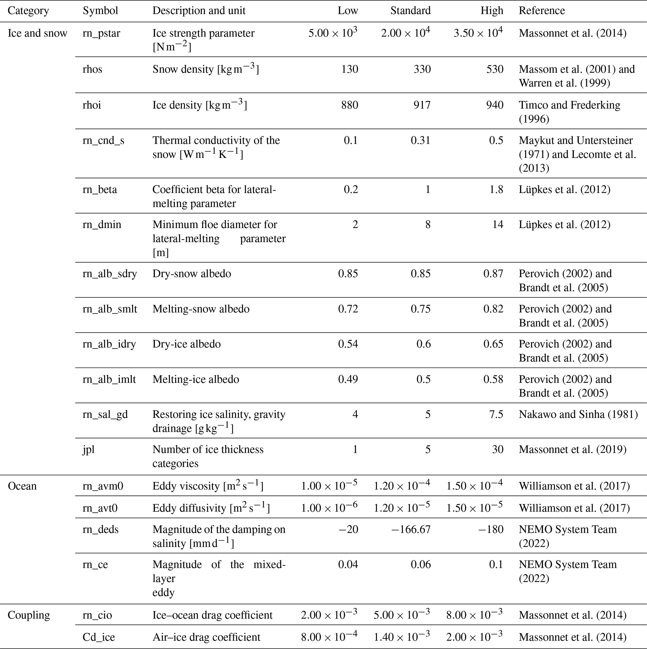
To investigate the sensitivity of sea ice budgets, we selected 18 parameters and determined their uncertainties (Table 1), which cover a number of important processes in sea ice modelling, such as ice and snow physical properties, ocean mixing and eddies, and ice–ocean and air–ice interactions. The lower and upper bounds of the parameters were selected according to the listed references, and the uncertainty intervals were suitably extended to avoid under-sampling at the edge of the interval. The standard values of the parameters used for the control experiment (CTRL) are the default values for NEMO4.0-SI³.

Table 1 The 18 parameters investigated, including their realistic ranges taken from the listed references.

2.2 Experimental design

The flow chart describing the procedure for obtaining the optimized model parameter values based on evaluation metrics is shown in Fig. 1. We start with the definition of the 18-dimensional parameter space (as already done in Table 1); the next steps are to sample from this parameter space and to run the NEMO4.0-SI³ model with a limited number of sampled sets of parameter values (the sampling method is described in the next section). Three sets of metrics are then calculated from the NEMO4.0-SI³ model output: (1) the area integrals of SIC budget components, (2) the area integrals of SIV budget components, and (3) the root-mean-square errors (RMSEs) between the simulated and observed SIC budgets (RMSE_SICB).

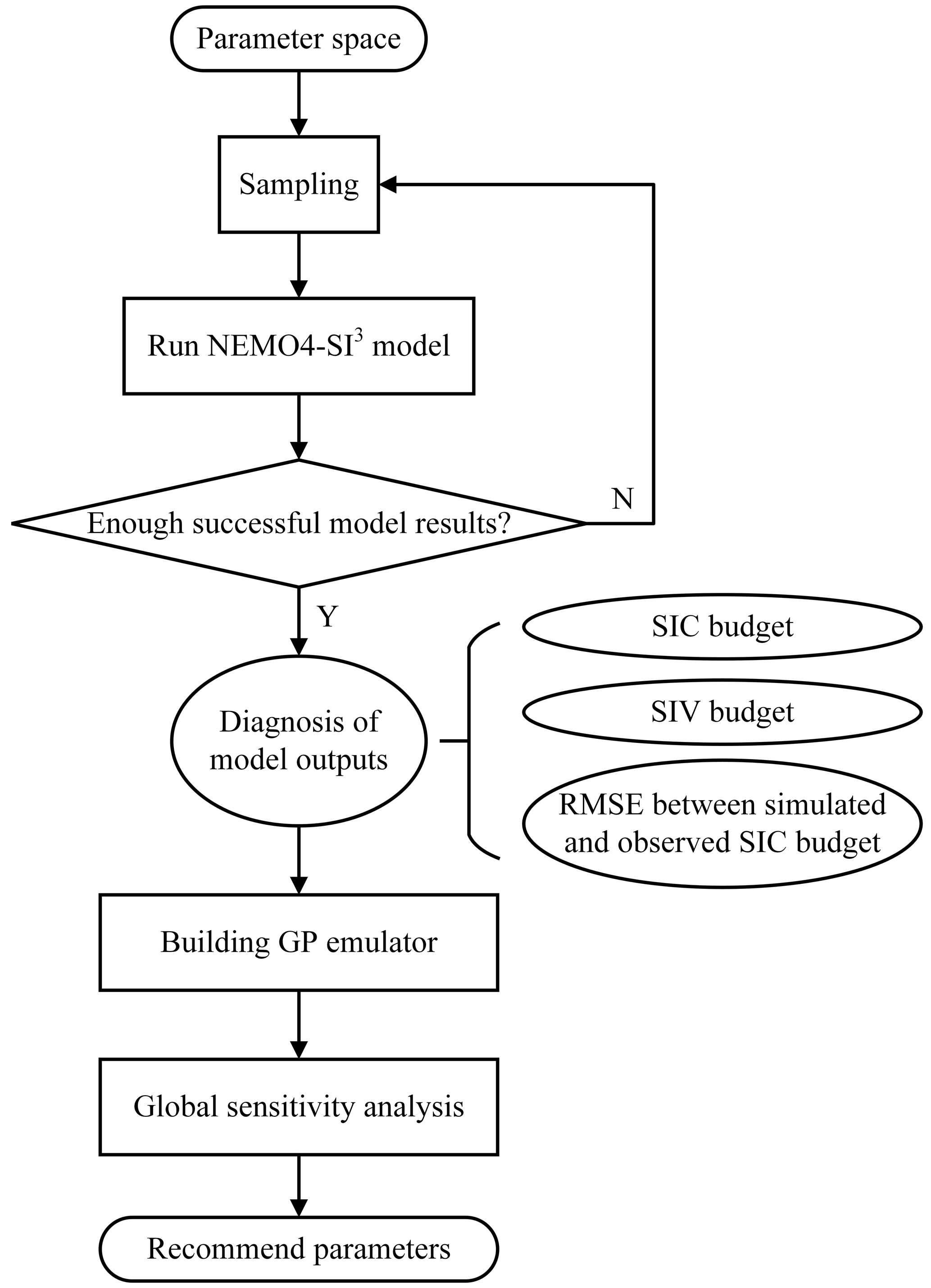
Figure 1 Flow chart describing how to obtain optimized parameter values for the NEMO4.0-SI³ model.

After the calculation of the three sets of metrics, GP emulators are trained (to be described in Sect. 2.4) to link the parameter sets with the evaluation metrics based on the NEMO4.0-SI³ simulations. Two GSA methods are used, the PAWN method (Pianosi and Wagener, 2015) and the Sobol method (Sobol, 2001; both described in Appendix A), with a large amount of input data to comprehensively explore the full parameter space covered by NEMO4.0-SI³ simulations and complemented by the GP emulators. Finally, once the key parameters have been identified by the GSA methods, parameter sets that provide results closest to the observations can be identified.

2.3 Latin hypercube sampling

We use the Latin hypercube sampling (LHS) method with a max–min property to generate low-discrepancy sequences from the 18-dimensional parameter space (step 2 in Fig. 1) to identify parameter set values for the NEMO4.0-SI³ simulations. The LHS is a stratified sampling method that divides each dimension evenly to ensure that samples are available in all intervals and therefore allows for a more evenly drawn sample than the usual random sampling methods (Morris and Mitchell, 1995; McKay et al., 2000). Additionally, the max–min property is a space-filling criteria that aims to maximize the minimum Euclidean distance between two sampling points and thus improves the effectiveness of the GP emulation (Joseph and Hung, 2008) to be carried out after the NEMO4.0-SI³ simulations. The recommendation for the number of samples to build a GP emulator is N=10p (Loeppky et al., 2009), where p is the dimension of parameter space and is equal to 18 in this study. In practice, however, we decided to use about 20p samples in order to build the GP emulator as accurately as possible (Williamson et al., 2017). Based on this principle, and taking into account possible model run failures, we first perform a sampling of 800 points in parameter space to run the NEMO4.0-SI³, and if the number of successful experiments ends up being too little (less than 360), we will continue the sampling.

2.4 Gaussian process emulator and model selection

The amount of computation using NEMO4.0-SI³ required to cover comprehensively the 18-parameter space for the model evaluation remains practically too large, and the use of a much faster GP emulator is required to emulate the behaviour of NEMO4.0-SI³ given the 18 parameter values. The emulator functionality is described next.

Let $X_{\mathrm{t}}=({\mathit{x}}_{\mathrm{1}},{\mathit{x}}_{\mathrm{2}},\mathrm{\cdots },{\mathit{x}}_N{)}^T$ and ${\mathit{Y}}_{\mathrm{t}}=(y_{\mathrm{1}},y_{\mathrm{2}},\mathrm{\cdots },y_N{)}^T$ denote the total number of N simulations; each x_i is a column vector of 18 values, sampled from the 18-dimensional parameter space by the LHS, and each y_i is a real number representing the corresponding model output metric, which is assumed to be noiseless here. A GP emulator f(⋅) for a model output metric Y_t=f(X_t) can generally be represented as

$$\begin{array}{}\text{(1)}& f(\cdot )\sim \text{GP}\left(\mathit{\mu }\right(\cdot ),K(\cdot ,\cdot \left)\right),\end{array}$$

where μ(⋅) and $K(\cdot ,\cdot )$ are prior mean function and covariance function respectively. Then the posterior distribution for parameter values X^∗ can be obtained as

$$\begin{array}{}\text{(2)}& f\left({\mathbf{X}}^{\ast }\right)\mathrm{|}f\left({\mathbf{X}}_{\mathrm{t}}\right)\sim N({\mathit{\mu }}^{\ast },K^{\ast }),\end{array}$$

where

$$\begin{array}{}\text{(3)}& {\displaystyle }{\mathit{\mu }}^{\ast }=\mathit{\mu }+K(X^{\ast },X_{\mathrm{t}})K(X_{\mathrm{t}},X_{\mathrm{t}}{)}^{-\mathrm{1}}(f\left(X_{\mathrm{t}}\right)-\mathit{\mu }),\text{(4)}& {\displaystyle }{K}^{\ast }=K(X^{\ast },X^{\ast })-K(X^{\ast },X_{\mathrm{t}})K(X_{\mathrm{t}},X_{\mathrm{t}}{)}^{-\mathrm{1}}K(X_{\mathrm{t}},X^{\ast }).\end{array}$$

We used the GPy software (GPy, 2012), with the prior of the mean function set to zero by default, and the user only had to choose the covariance function K to build the GP emulator for each evaluation metric. To achieve this, we used a 10-fold cross-validation method for model selection (Geisser, 1975). The idea is to divide the dataset {X_t,Y} evenly into 10 parts, each time using 9 parts as the “training data” to train the emulator and 1 part as the “true data” for model validation and so on for 10 cycles, taking the average as a proxy for model performance. Using this approach, we traversed the linear, squared exponential, exponential, Matern 3/2 and Matern 5/2 covariance functions and their sums and products (Rasmussen and Williams, 2006) for a total of 177 different combinations and then selected the covariance function with both the minimum RMSE and the highest correlation coefficient between the simulated and emulated values.

2.5 Sea ice concentration and volume budgets

Following the ice conservation law, the change of a sea ice state field Θ, such as SIC and SIV, can be attributed to dynamic and other processes (Leppäranta 2011, chap. 3.4):

$$\begin{array}{}\text{(5)}& {\displaystyle \frac{\partial \mathrm{\Theta }}{\partial t}}=-\mathbf{u}\cdot \mathrm{\nabla }\mathrm{\Theta }-\mathrm{\Theta }\mathrm{\nabla }\cdot \mathbf{u}+(f-r)\end{array}$$

where u is the sea ice velocity, f represents the change from freezing or melting, and r stands for any other processes (e.g. ridging and rafting). Integrating Eq. (5) over time, then the net changes in Θ over a period of time (t₂−t₁) can be obtained as follows:

$$\begin{array}{}\text{(6)}& \underset{t_{\mathrm{1}}}{\overset{t_{\mathrm{2}}}{\int }}{\displaystyle \frac{\partial \mathrm{\Theta }}{\partial t}}\mathrm{d}t=-\underset{t_{\mathrm{1}}}{\overset{t_{\mathrm{2}}}{\int }}\mathbf{u}\cdot \mathrm{\nabla }\mathrm{\Theta }\mathrm{d}t-\underset{t_{\mathrm{1}}}{\overset{t_{\mathrm{2}}}{\int }}\mathrm{\Theta }\mathrm{\nabla }\cdot \mathbf{u}\mathrm{d}t+\underset{t_{\mathrm{1}}}{\overset{t_{\mathrm{2}}}{\int }}(f-r)\mathrm{d}t,\end{array}$$

where the term on the left-hand side is the change or dadt (also referred to specifically as $\mathrm{d}C/\mathrm{d}t$ and $\mathrm{d}V/\mathrm{d}t$ for changes in SIC and SIV respectively), and the first term on the right-hand side represents the contribution of advection (adv), the represents the contribution of divergence (div), and the last term represents the residual (res). A positive value for each term is defined as an increase of Θ, and a negative value is defined as a decrease.

The budgets for SIC and SIV were calculated in our study, including seasonal climatologies for each SIC or SIV budget term, following the same approach as Holland and Kimura (2016). First, the daily dadt was obtained by central differencing of the ice fields on the day before and the day after; the advection and divergence were first calculated on each day and then averaged over the corresponding 3 d periods to be consistent with the daily dadt. Second, adv and div were subtracted from the dadt to obtain the daily res; and finally, all daily terms were summed over each season and averaged over the years 2008–2017.

2.6 Observational data

Daily sea ice velocity observations from Kimura et al. (2013), hereafter referred to as KIMURA, and SICs from the National Oceanic and Atmospheric Administration/National Snow and Ice Data Center (NOAA/NSIDC) Climate Data Record of Passive Microwave Sea Ice Concentration, version 4 (Meier et al., 2021; hereafter referred to as CDR) were used to calculate the observed SIC budget. The ice velocity dataset KIMURA was generated from the brightness temperature of the 36 GHz channel of the Advanced Microwave Scanning Radiometer-Earth Observing System (AMSR-E) using the maximum cross-correlation technique (Kimura et al., 2013) and ultimately deriving a 60 km resolution product. Therefore, the KIMURA data share the same period as AMSR-E and its successor AMSR2, covering from 2002 to the present. Following Holland and Kwok (2012), a 3×3 grid filter was used in the calculations to smooth out the grid-scale noise present in the satellite-derived ice drift. Regarding the SIC satellite observations, the CDR SIC is a rule-based combination of the NASA Team (Cavalieri et al., 1984) and NASA Bootstrap (Comiso, 1986) ice concentration datasets in the same 25 km×25 km grid, covering the years from 1978 to 2021, with daily, grid-based uncertainty estimates. The other three SIC observational products are only used as references in the calculation of SIE (integral of grid cells areas where SIC >15 %) and SIA (integral of grid cells areas multiplied by the SIC in each grid cell); they are AMSR-E and AMSR2 provided by NSIDC (Cavalieri et al., 2014; Meier et al., 2018), Ocean–Sea Ice Satellite Application Facilities (OSISAF) from the Copernicus Marine Service, and CERSAT developed by the French National Institute for Ocean Science (IFREMER; Ezraty et al., 2007).

The observed SIC budget (Fig. B1) shows that the Southern Ocean sea ice is generally transported to the ice edge at lower latitudes by advection and melts there, while divergence yields open water and thus promotes freezing of ice (Holland and Kwok, 2012; Uotila et al., 2014). It is important to note that the calculated SIC budget observations were considered to be “true values” in our study despite the uncertainties and biases in the ice drift observations, such as the overall overestimation of 5 % compared to the buoy-measured velocities (Kimura et al., 2013). The simulated SIC budgets and the root-mean-square errors from the observed one were only calculated at grid points with SICs larger than 15 % and at dates where ice drift observations existed to minimize the uncertainty of results caused by missing observations and observational errors.

3 Results

3.1 Sea ice concentration and thickness in the model ensemble

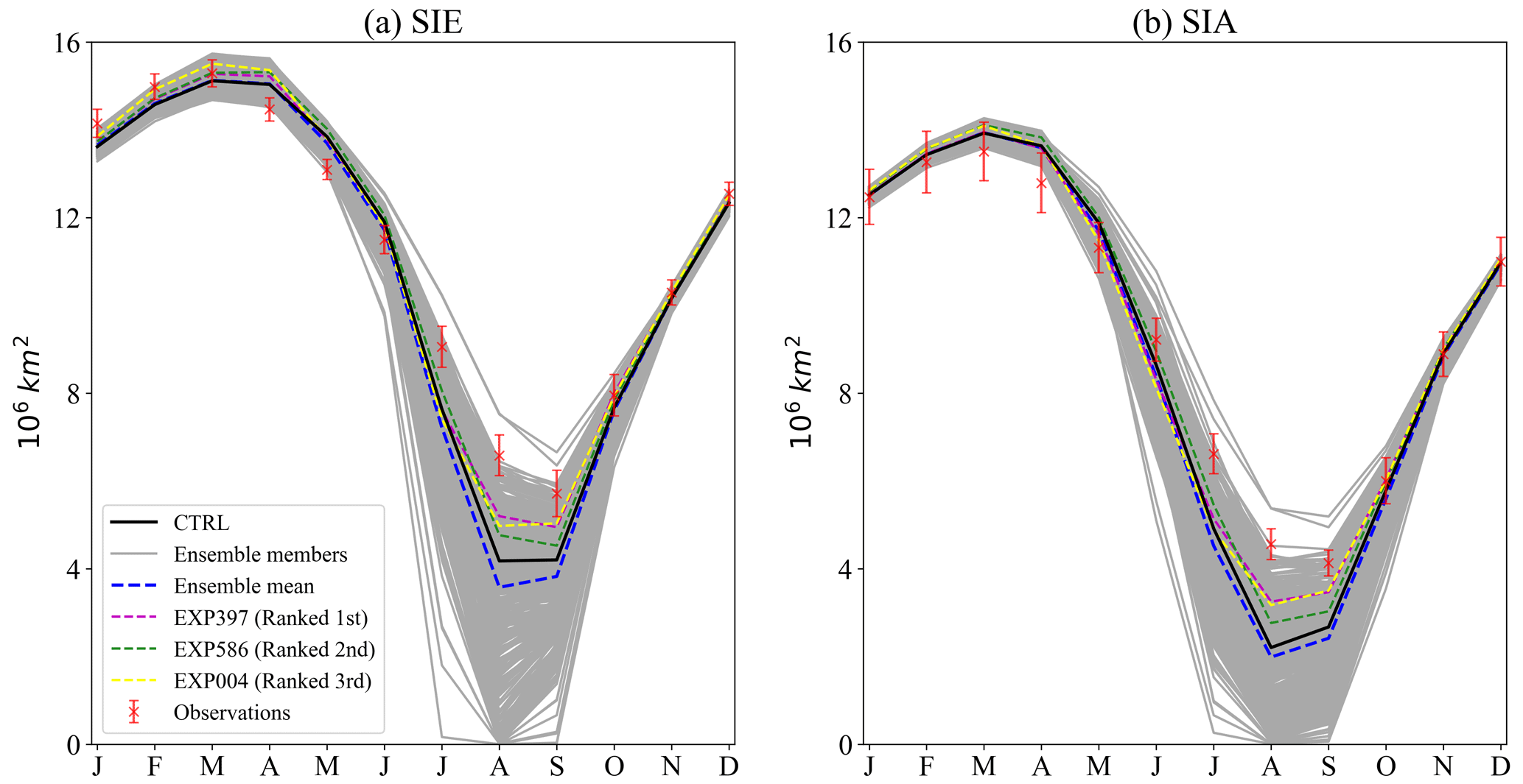
Out of 800 experiments, 44 % were terminated due to model instability caused by parameter combinations, resulting in an ensemble of models of size 449, which included the CTRL experiment. The seasonal cycles of SIE and SIA for the model ensemble are shown in Fig. 2. The SIE and SIA intervals for the ensemble cover the observed values fairly well, except for September, when SIA is systematically slightly overestimated. Inter-model disagreement due to parameter uncertainty is greatest in summer (ranging from 0.42 to 8.26×10⁶ km²), when SIE and SIA are at a minimum (observed at 4.26×10⁶ km²), while there is little disagreement between models during the autumn months. Among the members of the model ensemble, the CTRL run essentially overlaps with the ensemble mean and matches well with the observations.

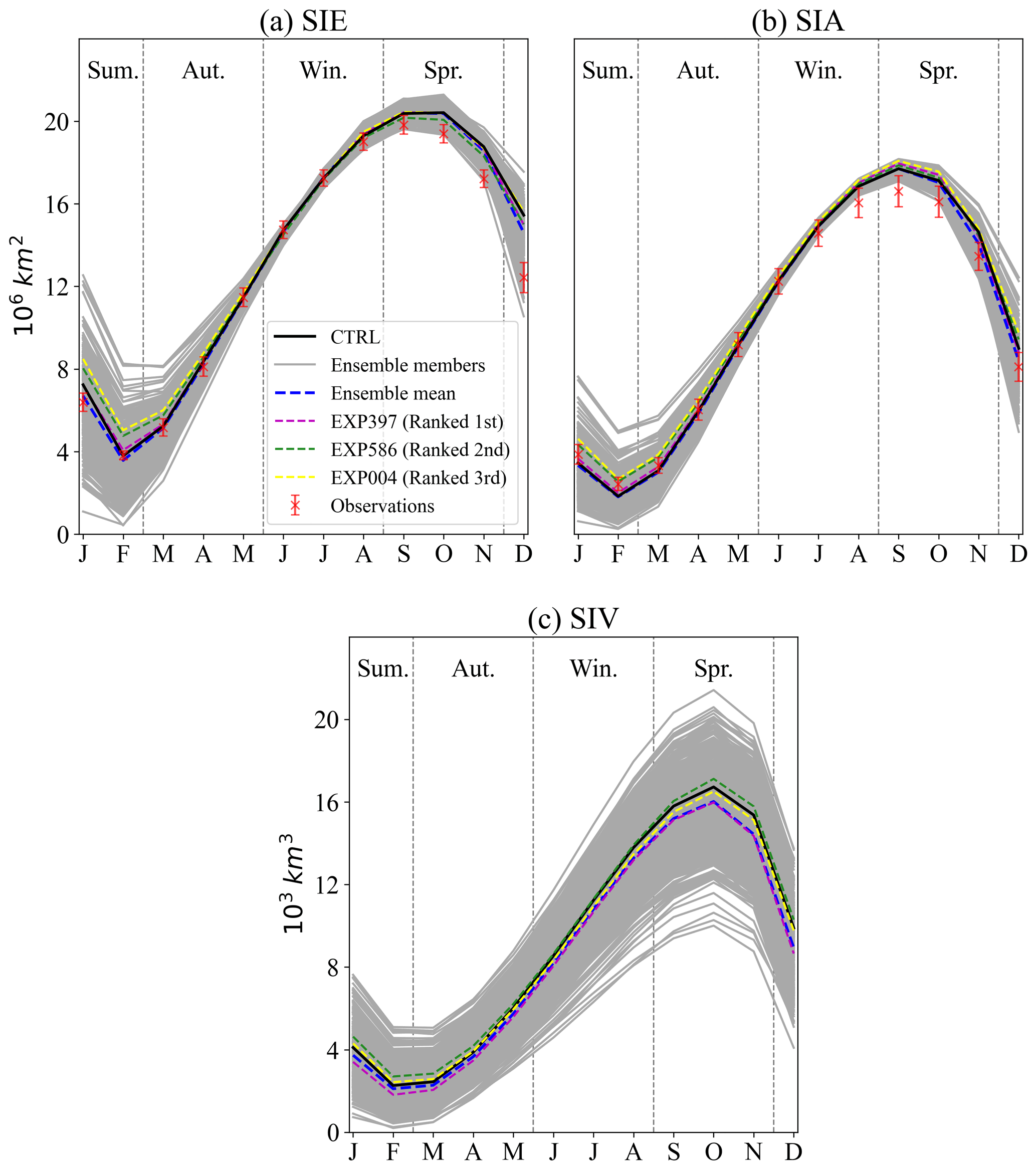
Figure 2 Simulated monthly climatologies of (a) sea ice extent (SIE), (b) area (SIA) and (c) volume (SIV) from 2008 to 2017; ensemble model means and results from four sets of experiments of interest are also highlighted. The SIE and SIA calculated from the CDR, AMSR-E and AMSR2, CERSAT, and OSISAF are used as references in the form of mean ± 1 deviation.

In February, comparing the ensemble mean SIC (Fig. B2a and b) with the CDR observation shows that there are still challenges in the modelling of the local patterns, especially as the NEMO4.0-SI³ significantly underestimates the SIC near the East Antarctic coast. In addition, the ensemble standard deviation for February stands at a high level (around 20 %) in most regions. On the other hand, in September (Fig. B2d–f) the ensemble mean SIC is more consistent with the observations than it is in February, although differences between the ensemble members remain relatively high (around 10 %) in marginal ice areas where the SIC is low. Overall, the discrepancies between ensemble members due to parameter uncertainty are smaller in high-SIC areas (SIC>90 %) than in low-SIC areas.

Similarly to the seasonal cycles of SIE and SIA, the CTRL run's SIV remains close to the ensemble mean. However, the differences between SIVs simulated based on different parameter sets are much greater than for SIEs (Fig. 2c) – for instance, in winter, the maximum values of SIVs in the ensemble members are more than twice as large as the minimum values. Additionally, the SIV cycles show a larger spread in winter than in summer, which is opposite to that of SIE cycles. For the ensemble mean sea ice thickness, thicker sea ice of up to 2 m is maintained year-round in the western Weddell Sea (Fig. B3a and c), which appears to be higher than the previous observation-based dataset of 1.2 to 1.5 m (Haumann et al., 2016, in their Extended Data Fig. 2). However, there is a lack of observations from the same period, as this study precludes a direct comparison. The spatial pattern of ice thickness standard deviation between model ensembles (Fig. B3) is similar to that of sea ice thickness, which means thicker sea ice is usually accompanied by a larger standard deviation.

3.2 Sea ice concentration and volume budgets in the model ensemble

The diagnostics of the SIC and sea ice thickness of the model ensemble in the last section show that the NEMO4.0-SI³ model driven by DFS5.2 provides reasonable results. The mean states of the model ensemble being close to the CTRL experiment, particularly for SIC, matches the observations very well, which provides a good basis for the budget analysis. In this section, we first calculated the SIC budget and SIV budget for the ensemble of 449 model runs by applying the same approach as for the calculation of the observed SIC budget (see Fig. B1) and then computed the RMSE_SICB (step 5 in Fig. 1).

3.2.1 Model ensemble mean and standard deviation

As can be seen in Fig. 3, the spatial-pattern characteristics of the ensemble mean of $\mathrm{d}C/\mathrm{d}t$ and adv for each season are generally consistent with observations. The magnitudes of the model ensembles of $\mathrm{d}C/\mathrm{d}t$ and adv are significantly larger due to the fact that the observed ice drift has some missing values and that the $\mathrm{d}C/\mathrm{d}t$ term is only integrated over the grids with ice drift observations. However, the simulated divergence appears to be systematically biased when compared to the observational data; the simulated div in the inner ice pack is smaller than the observed one, even considering there are missing data in the observations; and some sporadic convergence (positive value of divergence) scattered in the marginal ice zone is not captured by the model. The lack of divergence in the inner ice pack also leads to a lack of open water and thus insufficient freezing of sea ice, which can be seen from the winter and spring res in Fig. 3 and in summer in the south Weddell Sea. In summer, the overall contribution of model-simulated advection and divergence to sea ice change is minimal, with thermodynamic sea ice melt dominating, which is consistent with the observational data.

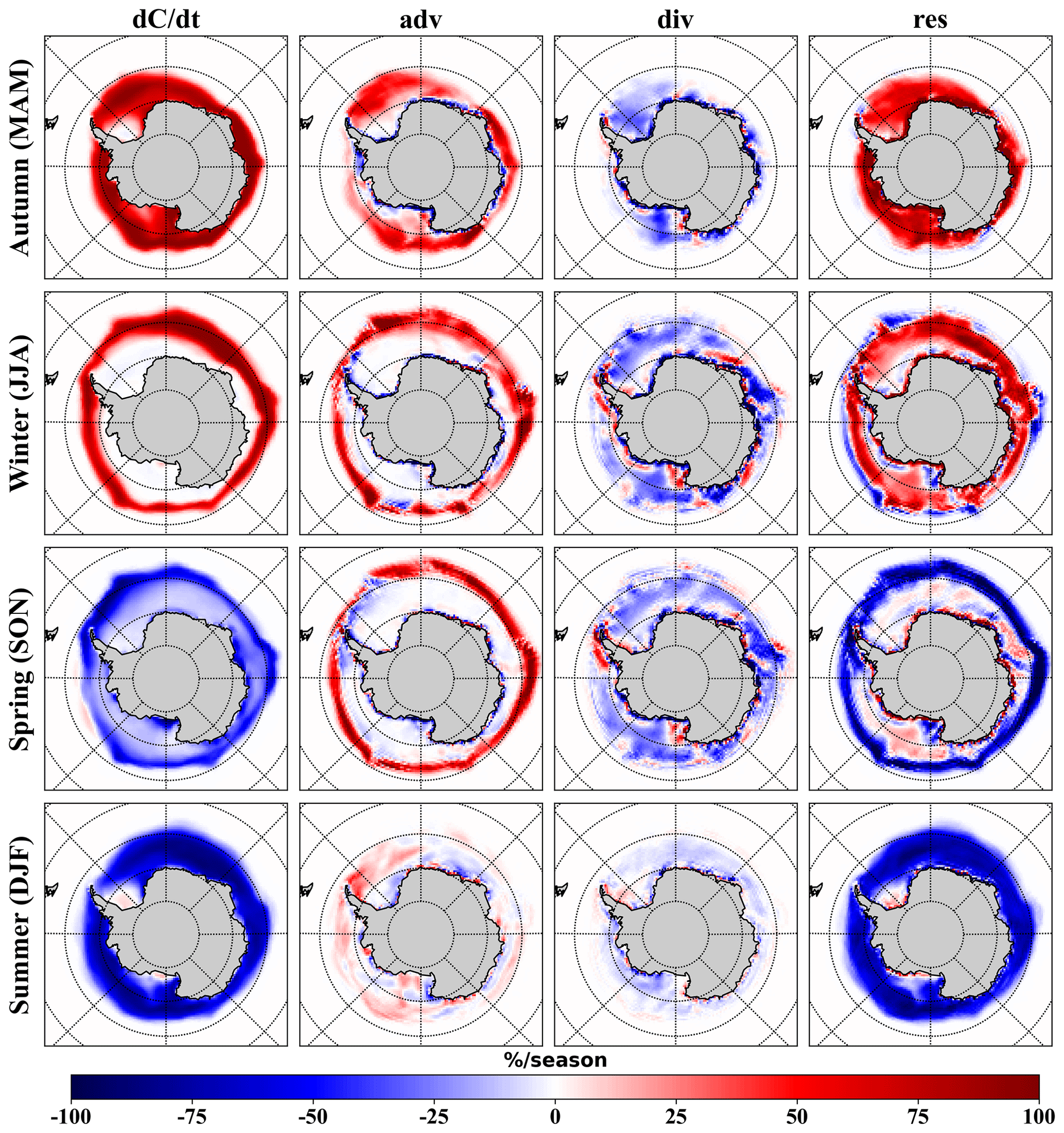
Figure 3 Mean seasonal SIC budget components for the ensemble of 449 model runs from 2008 to 2017. The specific meaning of each term has been described in Sect. 2.5. A positive or negative percentage value indicates an increase or decrease in SIC during the season. The first column is the sum of other columns. The SIC budget for each member was first calculated separately and then averaged together.

The standard deviation of each budget term for the model ensemble was also calculated (Fig. 4); the deviations between simulated sea ice changes are mainly concentrated in autumn and summer and are mainly located in the Weddell and Ross seas, with insignificant deviations in winter and autumn. For the advection term, the inter-model deviation is large at the ice edge, where sea ice is transported by the advection, and in the coastal area, where winds and currents are strong. The deviations of the divergence term in the model ensemble are mostly concentrated in the coastal region, while the model ensemble is more consistent in the inner ice pack, although the greatest differences between simulations and observations are found there. Since the res term was calculated by subtracting adv and div from $\mathrm{d}C/\mathrm{d}t$, the deviations in these three terms are generally combined in the res term, with the possible exception of some cancelling-out of deviations in these terms – for example, in the Weddell Sea, in autumn, res deviates less than $\mathrm{d}C/\mathrm{d}t$.

Figure 4 Standard deviation of seasonal SIC budget components for the ensemble of 449 model runs. The maximum value of the colour map is limited to 30 % per season for the best presentation. A higher percentage value means that the model ensemble is more divergent here.

The SIV increases extensively in the Southern Ocean in autumn and winter and decreases in summer ($\mathrm{d}V/\mathrm{d}t$ column in Fig. 5) and generally decreases in spring, except for a slight increase in the Amundsen–Bellingshausen seas and along the south Weddell Sea. Differing from the SIC budget (Fig. 3), in which advection contributes little to sea ice changes in the inner ice pack, the ensemble model mean shows that advection will lead to a reduction in SIV (adv column in Fig. 5), although SIC remains high in this region. The spatial pattern of the divergence of SIV does not differ much from that of SIC, and since the contribution of simulated SIC divergence to sea ice change is underestimated compared to the observational data, as mentioned earlier, it is safe to assume here that divergence should similarly underestimate the change in SIV, given the strong interdependence of SIC and SIV. The inner ice pack maintains an increase in SIV from autumn to spring as the sea ice freezes, and from spring onwards, the sea ice starts to melt from the marginal ice zone and reaches a full melting of all the Southern Ocean sea ice in summer (res column in Fig. 5).

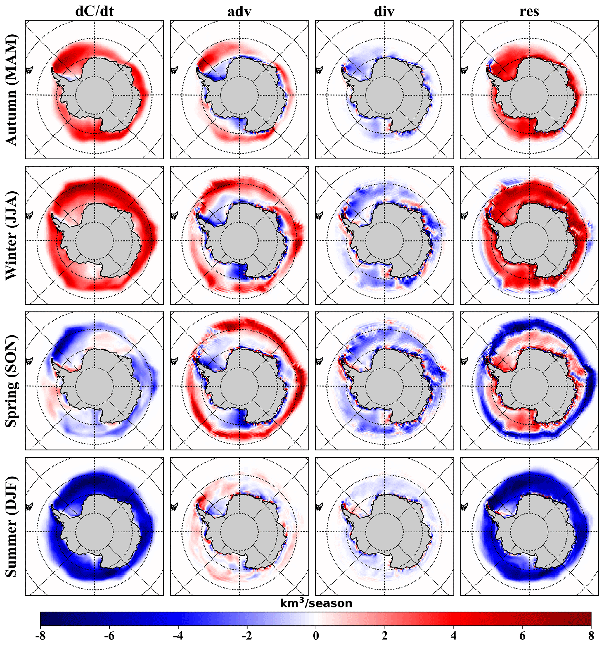
Figure 5 The same as Fig. 3 but for SIV budget. A positive or negative value indicates an increase or decrease in SIV, respectively.

For simulations of overall changes in SIV, the standard deviation between ensemble members is only slightly greater in summer than in other seasons (Fig. 6). The disagreement between members originates mainly from the contribution of advection to SIV change, which is most pronounced along the west Weddell Sea and Antarctic Peninsula coasts, in marginal ice zones, and along the East Antarctic coast. In addition, the contribution of advection and divergence to SIV that is simulated based on different parameter sets varies considerably in the Antarctic coastal region, similar to the SIC budget. The residual term, which equals the thermodynamic contribution as SIV is conserved, still has the largest standard deviation, as it retains the deviations of the other terms.

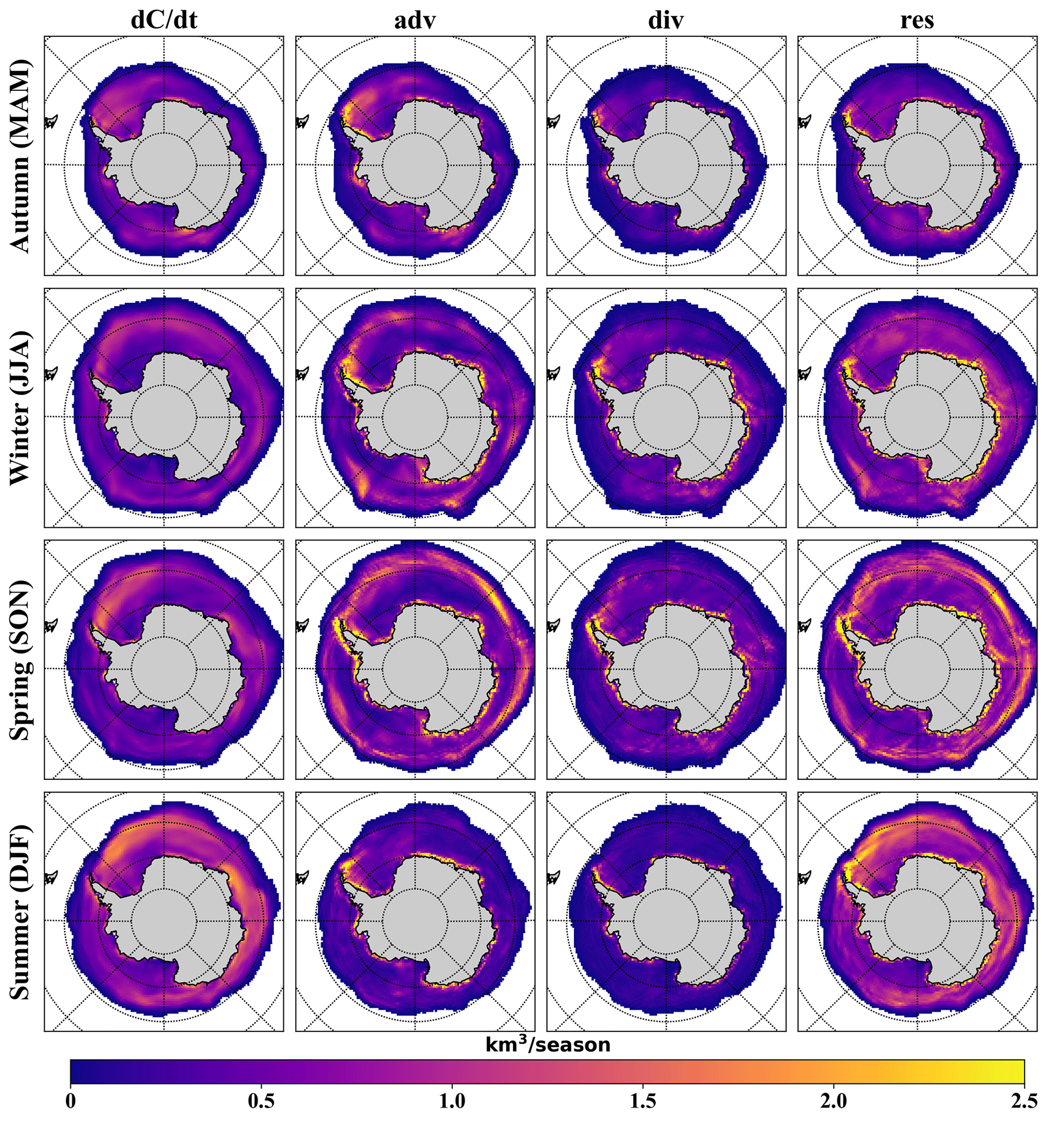
Figure 6 The same as Fig. 4 but for SIV budget. The maximum value of the colour map is limited to 2.5 km³ per season for the best presentation.

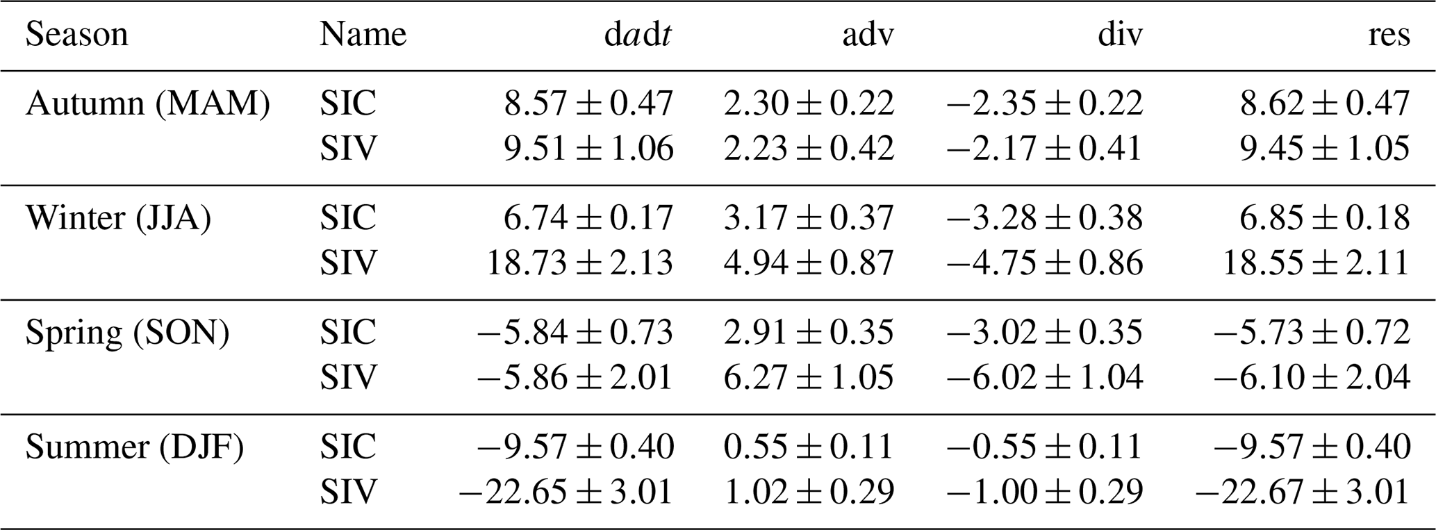
The area and time integrals of each budget term for the simulated SIC and SIV are presented in Table 2. Although this quantification of the contribution of each term to sea ice change does not consider local differences and cancels out positive and negative sea ice change to some extent, it is a simple and easy-to-implement method for quantifying the sensitivity of the sea ice budget to parameters. As can be seen from the ensemble mean of SIC and SIV budget terms, the area integrals of the advection and divergence contributions to sea ice change largely cancel each other out. For SIV, this is because these two processes do not change the total amount of sea ice, and for SIC, this also holds approximately, considering that in the Southern Ocean sea ice is close to free drifting, and the non-conservative nature of SICs due to ridging can be neglected (Uotila et al., 2014; Holland and Kimura, 2016). Therefore, when studying the effects of model parameter uncertainty on sea ice budgets in the following sections, it is necessary to only use the area integrals of res (or dadt) and adv (or div).

Table 2 Area integrals of sea ice concentration (SIC) and sea ice volume (SIV) budget components for the ensemble of 449 model runs. Data are listed in the form of mean ± 1 standard deviation. The units are 10⁶ km² and 10³ km³ for the SIC and SIV budget, respectively.

3.2.2 RMSEs between the simulated and observed SIC budgets

The RMSE_SICB is calculated as a complement to the area integrals of each SIC budget term. In matching the simulated results to the observational data, we first linearly interpolated the modelled data onto the grid cells containing observed data and then calculated daily budgets for only those dates for which observations were available and for grids with SICs greater than 15 %; finally, we calculated the seasonal SIC budget climatology. Figure 7 counts the RMSE_SICB for all model ensemble members. The model ensemble has the smallest RMSE_SICB with observations in terms of net sea ice change (∼15 %), followed by advection (∼25 %), and a larger RMSE_SICB for the divergence term, which is consistent with the results shown in Figs. 3 and B1. In the model ensemble, the RMSE_SICB of the CTRL experiment is essentially at or below the median level, and the distributions of the RMSE_SICB in the model ensemble are not symmetric; i.e. there are more flier points outside of the third quartile plus 1.5 times the inter-quartile range.

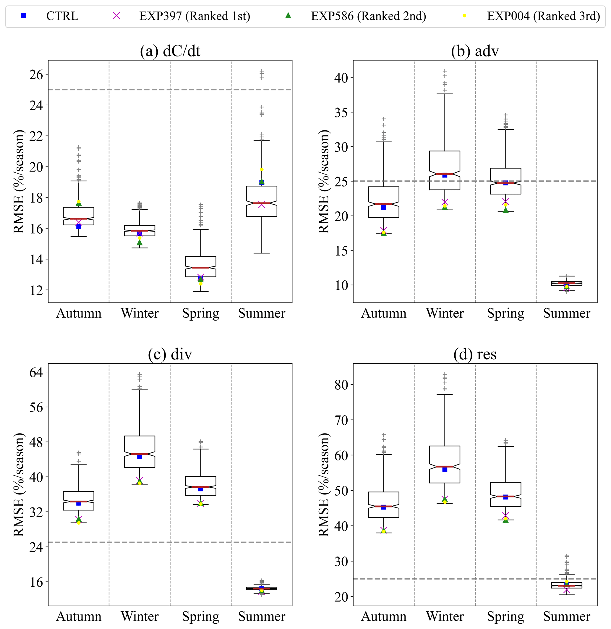
Figure 7 Boxplots of RMSE for each component of the simulated and observed SIC budget. Boxes extend from the first quartile (top border) to the third quartile (bottom border). The red line represents the median of all 449 model results. The CTRL experiment and three best-performing experiments are also flagged. The whiskers extend outwards from the box to 1.5 times the inter-quartile range, with a few flier points beyond the whiskers. The 25 % horizontal dashed lines are marked as references.

3.3 Sensitivity of ice concentration and volume budgets to parameters

Based on the results of the last section, the area integrals of adv and res in the SIC (and SIV) budget and the RMSE_SICB are used as the metrics to assess the sensitivity of the model's sea ice budget to 18 parameters in this section. Before conducting the GSA, Fig. B4 shows the cross-validation results for the best GP emulator for each of the adv and res term area-integral metrics of the SIC and SIV budgets (step 6 in Fig. 1). Overall, the emulated and simulated values have very high correlation coefficients (typically greater than 0.98); thus, the built emulator is considered successful and will be used as a proxy for NEMO4.0-SI³ in the subsequent sensitivity analysis.

The sensitivity of each metric of the 18 parameters, quantified by the Sobol and PAWN methods, is illustrated in Fig. 8. It should be noted that the sensitivity scores for the two methods are independent and not comparable in absolute terms. Following Urrego-Blanco et al. (2016), the Sobol sensitivity index below 0.02 is considered insignificant, and for the Kolmogorov–Smirnov (KS) mean index in PAWN, the critical value at a confidence level of 0.05 is about $\mathrm{6.65}\times {\mathrm{10}}^{-\mathrm{2}}$. Both GSA methods show that the advection is very sensitive to ice strength (rn_pstar) outside of summer in the SIC budget. Ice–ocean drag coefficients (rn_cio) and air–ice drag coefficients (Cd_ice) have an influence on the modelled advection contribution to sea ice change from summer to autumn and spring, respectively. In summer, the snow thermal conductivity (rn_cnd_s) and two lateral-melting parameters (rn_beta and rn_dmin) also have some effect on the advection of SIC budget. The total and first-order Sobol indices are not very different, which is usually the case for both indices of the PAWN method, with the exception of the number of ice thickness categories (jpl) where the KS max is shown to be much larger than the KS mean (e.g. in autumn and summer). For other metrics, this also happens for the sensitivity assessment of some other parameters, which will be discussed further in the next section. The residual term of the SIC budget shows considerable sensitivity to the ice–ocean drag coefficient (rn_cio), which persists from autumn to spring. Meanwhile, the effect of the air–ice drag coefficient (Cd_ice) on res increases continuously from autumn to summer. Ice strength still has a weak effect, much less of an effect than that on adv. In addition, snow thermal conductivity (rn_cnd_s) and number of ice thickness categories (jpl) have a non-negligible effect on the modelling of res in winter and summer, respectively.

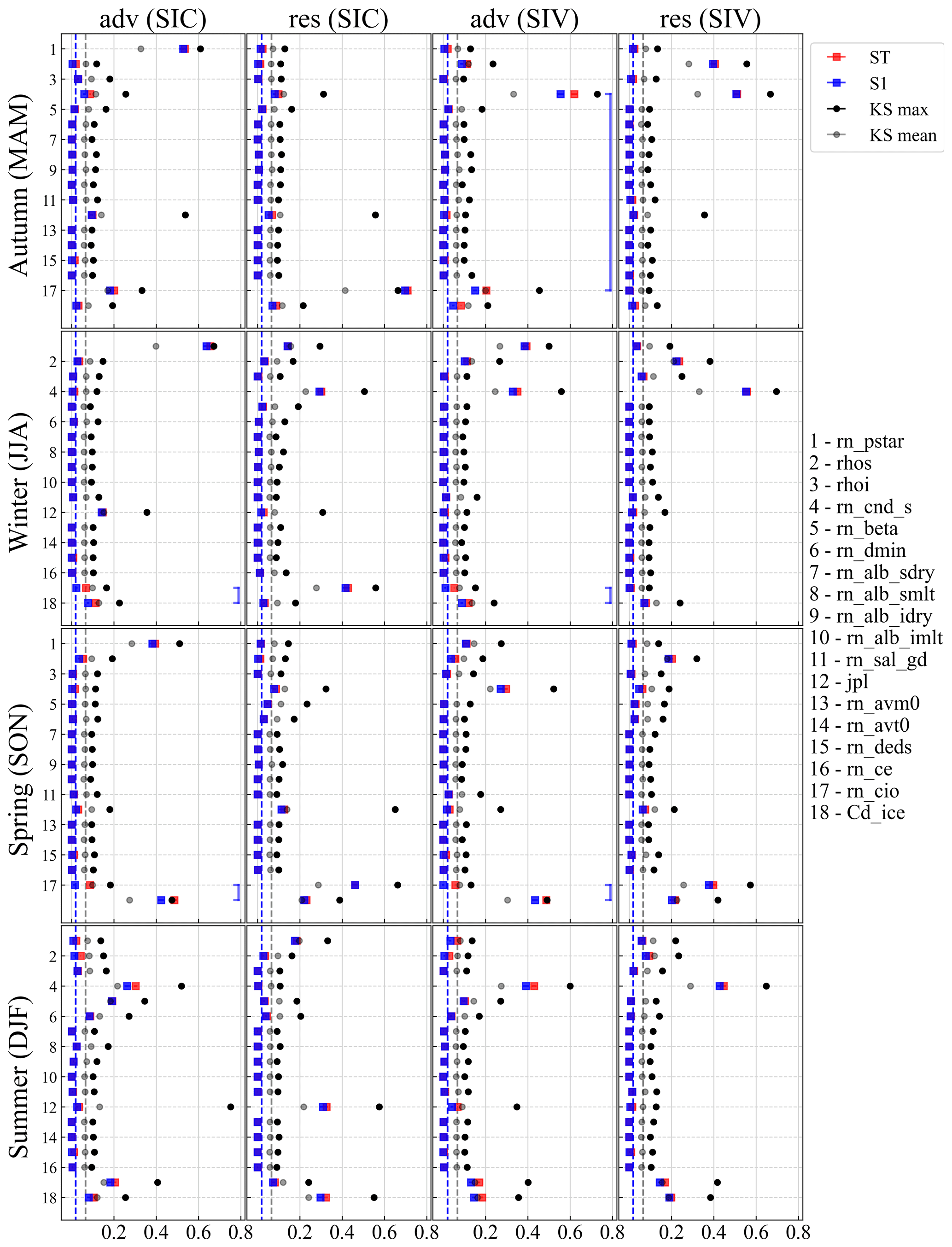
Figure 8 The total (ST) and first-order (S1) Sobol sensitivity indices and the maximum (KS max) and mean (KS mean) PAWN sensitivity indices for each sea ice budget component of 18 parameters. The dashed blue and grey lines are the thresholds for S1 and KS mean indices, respectively. Larger Sobol and PAWN index values indicate that the metric is more sensitive to this parameter. The blue connecting line indicates that the Sobol second-order index for the combination of these two parameters is greater than 0.02.

Among the sensitivity indices of the SIV budget, the most noticeable parameter is snow thermal conductivity (rn_cnd_s), to which both adv and res are very sensitive at all times of the year, except in the spring, when it has less impact on res (Fig. 8). Another physical parameter related to the snow on sea ice (rhos, i.e. snow density) is important for res simulations in the SIV budget, especially from autumn to winter, the period when sea ice freezes fast (Fig. 2c). Similar to the SIC budget, the air–ice and ice–ocean drag coefficients remain crucial for the SIV budget in spring and summer, while the ice strength is only important for advection in winter and spring.

3.4 Sensitivity of SIC budget errors to parameters

The results for four RMSE_SICB metrics based on the best-performing GP emulators are shown in Fig. B5. The GP emulator performs well for the RMSE_SICB of adv, div and res, with a correlation coefficient greater than 0.998, except in summer. As can be seen in Fig. 7, in the summer months, the difference in RMSE_SICB for these three terms is very small compared to in other seasons, and this small difference is likely to be random and therefore difficult for the GP emulator to capture well. The GP emulator also does not perform well in terms of $\mathrm{d}C/\mathrm{d}t$ RMSE_SICB (Fig. B5, first column), and there is also likely to be a large randomness in the difference in $\mathrm{d}C/\mathrm{d}t$ between the model ensemble and the observational data. Given the poor performance of the GP emulator in terms of $\mathrm{d}C/\mathrm{d}t$ RMSE_SICB, as well as in terms of RMSE_SICB over the summer, the GSA results obtained by using it instead of the NEMO4.0-SI³ dynamical ocean model are subject to uncertainty, and this should be kept in mind in the following analysis.

Figure 9 demonstrates quite clearly that for adv, div and res RMSE_SICB in autumn, winter and spring (which are also the terms and seasons with the largest RMSE_SICB values; Fig. 7), only air–ice and ice–ocean drag coefficients are the most critical parameters, while ice strength also has, but only weakly, an effect. Besides these two important drag coefficients, Fig. 9 also shows that the $\mathrm{d}C/\mathrm{d}t$ RMSE_SICB between model and observational data might be sensitive to the snow thermal conductivity and ice category number to some extent. The analysis is more complicated in summer, as is the sensitivity of the SIC budget and SIV budget to the parameters. In addition to all the previously mentioned parameters that have an impact, Fig. 9 shows that, in summer, the RMSE_SICB may also be sensitive to the minimum floe diameter for the lateral-melting parameter (rn_dmin) and the magnitude of the damping on salinity (rn_deds), which is a parameter belonging to the ocean module. Further comparing Figs. 8 and 9, it can be found that, overall, both the simulation of the SIC budget by the NEMO4.0-SI³ model and its RMSE_SICB are most sensitive to the air–ice and ice–ocean drag coefficients, both of which belong to the coupling category in Table 1. Also important are ice strength and the thermal conductivity of snow, identified by the six metrics related to SIC budget. In summer, some thermodynamic melting-related parameters, such as rn_beta (coefficient beta in the lateral-melting parameterization scheme) and rn_dmin (minimum floe diameter in the lateral-melting parameterization scheme), are important. In contrast, the SIC budget simulated by the model is sensitive to the number of ice thickness categories (jpl), unlike the RMSE_SICB metrics.

Figure 9 The same as Fig. 8 but for the sensitivity of the RMSE between SIC budgets of the model and the observational data to 18 parameters. The red connecting lines are the same as the blue ones but for the Sobol second-order index larger than 0.1.

As it has been identified that the RMSE_SICB metrics are sensitive to the two most critical parameters (air–ice and ice–ocean drag coefficients) and one relatively important parameter (ice strength), Fig. 10 illustrates the RMSE_SICB for all SIC budget terms and all seasons, averaged over 449 model runs, in relation to the values of these three parameters, with the top 10 combinations listed in Table 3. It can be seen in Fig. 10b that the RMSE_SICB broadly decreases with increasing ice–ocean drag coefficient (rn_cio) and decreasing air–ice drag coefficient (Cd_ice), such that the 10 sets of model runs with the smallest RMSE_SICB are concentrated in the top-left corner of the figure, where air–ice drag coefficient is from approximately $\mathrm{8}\times {\mathrm{10}}^{-\mathrm{4}}$ to $\mathrm{1}\times {\mathrm{10}}^{-\mathrm{3}}$ and where ice–ocean drag coefficient is from approximately $\mathrm{5.5}\times {\mathrm{10}}^{-\mathrm{3}}$ to $\mathrm{7.5}\times {\mathrm{10}}^{-\mathrm{3}}$ (Table 3). In contrast, the best 10 ice strength values are more dispersed and greater than 15×10³ (Fig. 10a and c), and the RMSE_SICB does not depend linearly on it, as with air–ice and ice–ocean drag coefficients (i.e. Cd_ice and rn_cio).

Table 3 The 10 best-performing experiments in terms of mean RMSE_SICB (i.e. RMSE between simulated and observed SIC budget) and the values of the three key parameters they used. Note that these values highly correspond to the DRAKKAR Forcing Set version 5.2 (Dussin et al., 2016) atmospheric forcing used in this study.

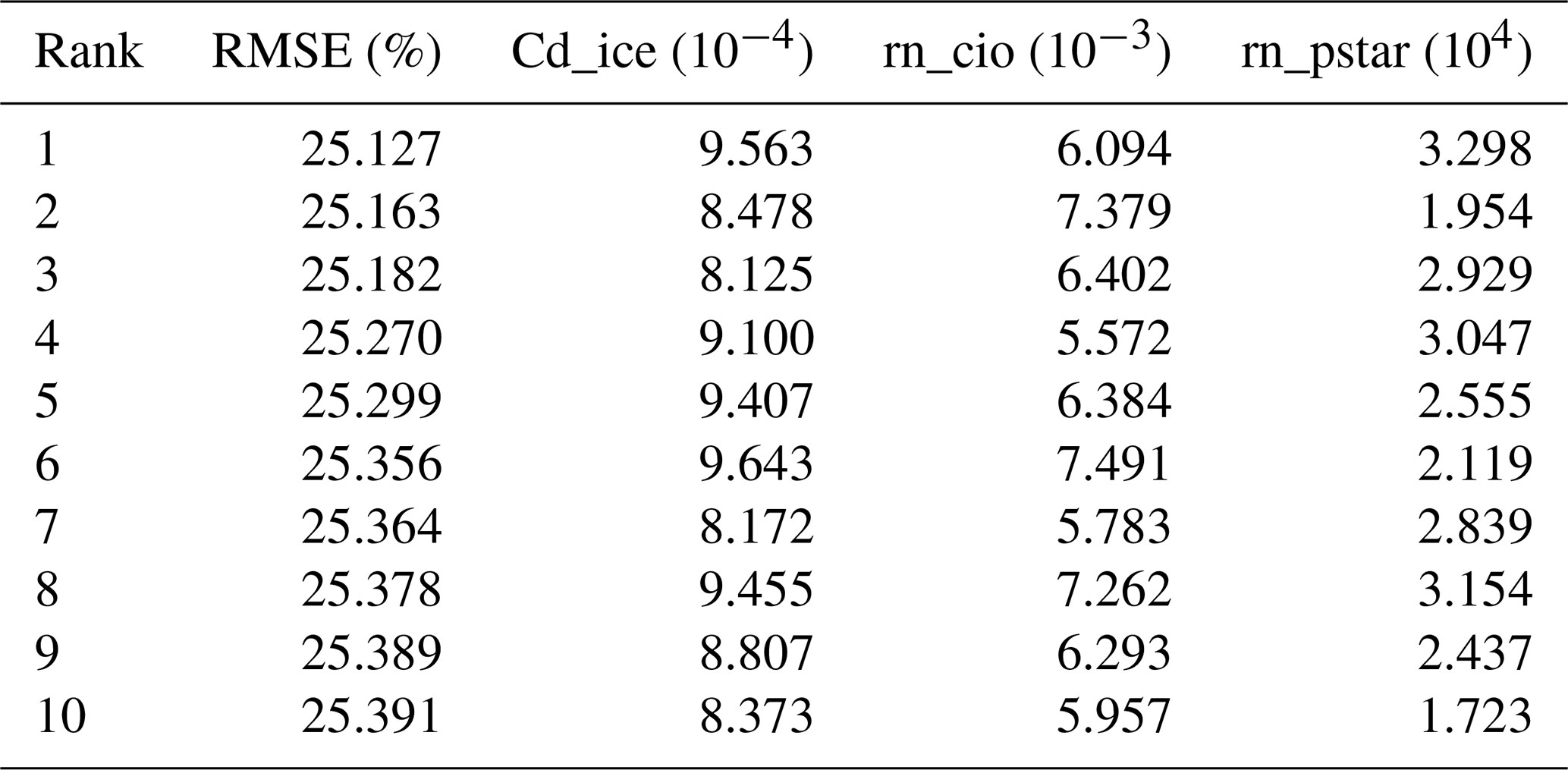
Figure 10 Average RMSE_SICB for all four SIC budget components for different combinations of key parameters. The numbers 1 to 10 indicate the results of the 10 best parameter sets in ascending order of the average RMSE_SICB, and the points with red edges indicate the standard values used for the CTRL experiment.

4 Discussion

4.1 Key parameters and their physical effects

Several parameters have been identified in Sect. 3.3 and 3.4 as having a significant impact on the simulated SIC and SIV budgets in the Southern Ocean. In this section, we present how these parameters specifically act on the SIC and SIV budget by looking at the impact of parameter changes on the cumulative distribution function (CDF) in the PAWN method.

Considering the performance of the GP emulator (Fig. B4), as well as the number of sensitive parameters (Fig. 8), the area integral of the res component in the SIC budget in spring and the area integral of the adv component in the SIV budget in winter have been selected here as examples to be discussed. Figures 11 and 12 show how the CDF of the model output changes as one parameter is fixed to vary across a range of values and as other parameters are varied freely.

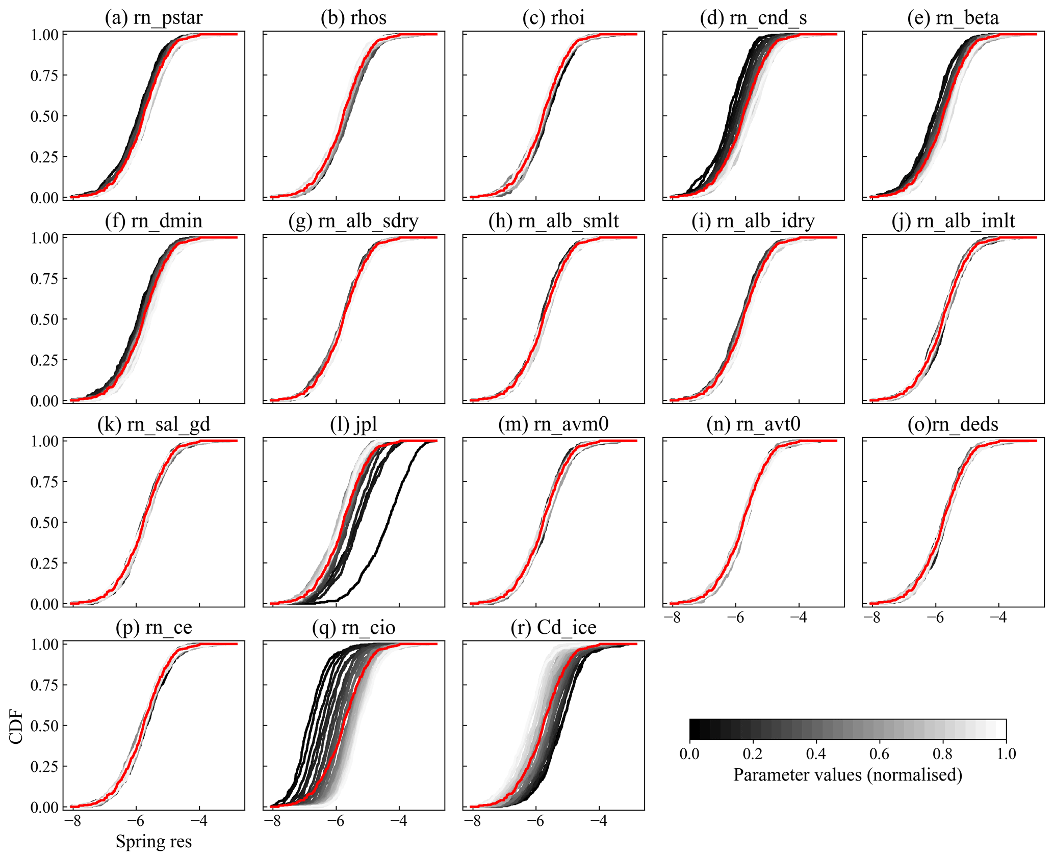
Figure 11 Cumulative distribution function (CDF) of the area integral of the res component in the spring SIC budget (see Fig. 3). Red lines are the unconditional CDF for the ensemble of 449 model runs, and the grey lines stand for conditional CDF at different fixed values of parameters calculated by the GP emulator. The units of the x axis are 10⁶ km².

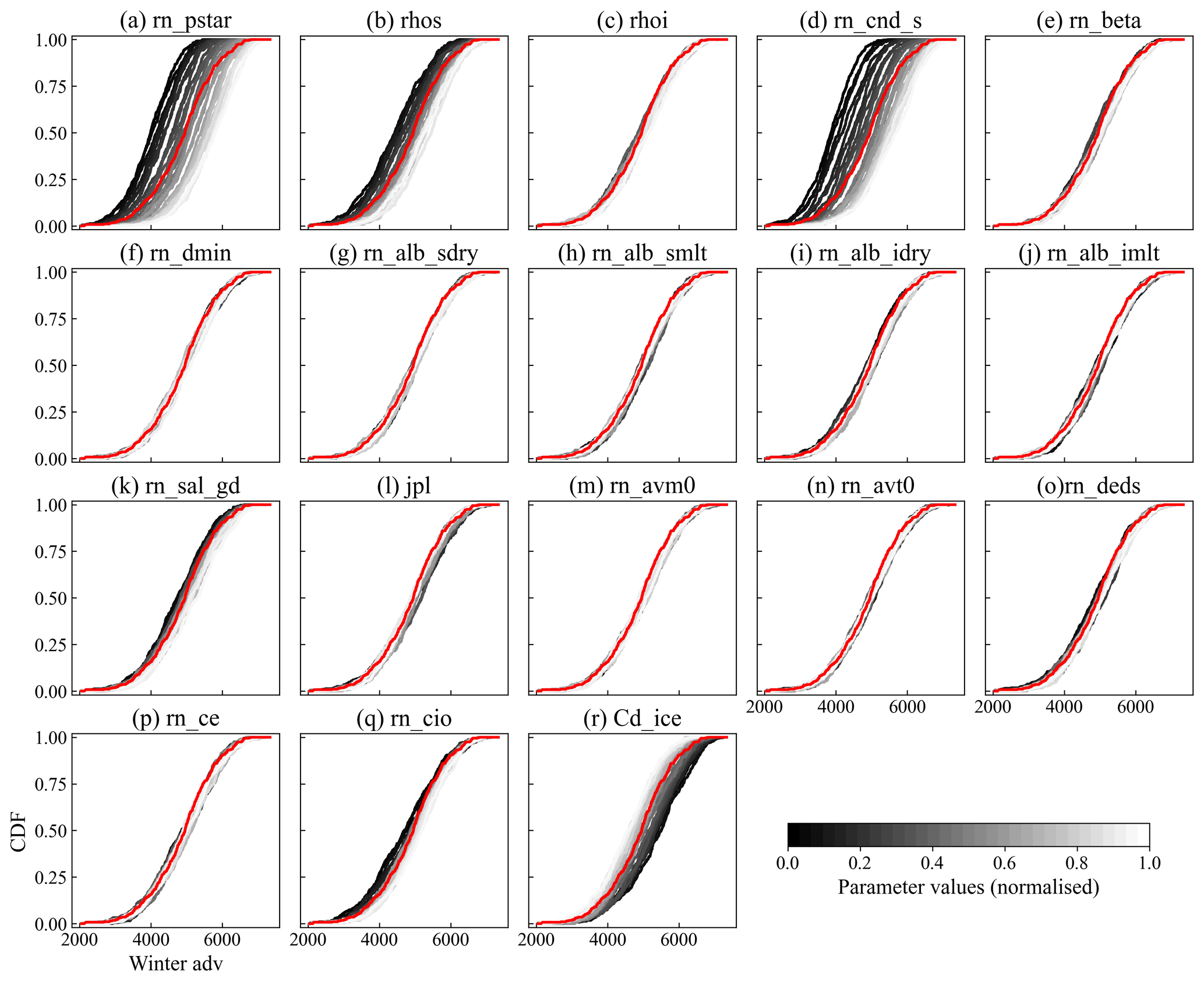
Figure 12 The same as Fig. 11 but for the area integral of the adv component of the winter SIV budget. The units of the x axis are 10³ km³.

Since the low thermal conductivity of the snow reduces the heat transfer from the bottom of the ice to the atmosphere, it reduces the ice growth rate (Fichefet et al., 2000; Lecomte et al., 2013) and therefore leads to less freezing inside the ice pack, and res moves more towards negative values (Fig. 11d). The reduction in freezing due to the reduction in snow thermal conductivity is more pronounced in winter (Fig. 8), and the SIV budget simulation is more sensitive to this parameter than the SIC budget is, as it primarily affects the vertical ice growth.

The rn_beta and rn_dmin are the two parameters that determine the minimum floe diameter of sea ice, and their decrease implies a decrease in sea ice floe sizes, which promotes the lateral melting (Lüpkes et al., 2012). Consequently, in contrast to the reduction of snow thermal conductivity (rn_cnd_s), which inhibits ice freezing, rn_beta and rn_dmin lead to more negative values of res (Fig. 11e and f) by promoting sea ice melting at low-latitude regions (Fig. 3). Furthermore, this effect is greater in summer than in spring and plays a weak role in winter (Fig. 8), which fits well with the magnitude of the SIC reduction in the res column in Fig. 3, although it is not the only process that affects SIC.

Compared to rather continuous-looking variations in CDFs of other parameters, the variation in CDFs due to changes in the number of ice thickness categories (jpl) is more dispersed (Fig. 11l), with several lines clearly being outliers, which were checked to match jpl=1. This is because the multi-category sea ice thickness takes into account the subgrid-scale variations in sea ice properties (Thorndike et al., 1975; Massonnet et al., 2019; Moreno-Chamarro et al., 2020) and is therefore significantly different from the single-thickness category (jpl=1). For instance, the presence of thin sea ice categories in multi-category sea ice schemes allows for greater melt rates compared to a single-category scheme (Uotila et al., 2017).

The ice–ocean drag coefficient and the air–ice drag coefficient should be discussed jointly, as the sea ice drift velocity is related to the Nansen number $\mathit{\text{Na}}=\sqrt{{\mathit{\rho }}_{\mathrm{a}}{C}_{\mathrm{a}}/{\mathit{\rho }}_{\mathrm{w}}{C}_{\mathrm{w}}}$, where ρ_a/w and C_a/w are air and water density and air–ice and ice–ocean drag coefficient. The Figs. 11q and r illustrate that a decrease in $C_{\mathrm{a}}/C_{\mathrm{w}}$ leads to a larger res, which has two possibilities: either sea ice melt is inhibited or freezing is intensified by assuming that sea ice deformation is comparably small (Holland and Kwok, 2012). Since the solution of free sea ice drift (Leppäranta, 2011, chap. 6.1.1) indicates that the decrease in $C_{\mathrm{a}}/C_{\mathrm{w}}$ leads to a decrease in sea ice velocity, we argue that this causes a more limited transport of sea ice to low-latitude regions, leading to the inhibited melting (see spring adv and res in Fig. 3).

With the exception of snow thermal conductivity (rn_cnd_s), ice–ocean drag coefficients (rn_cio) and air–ice drag coefficients (Cd_ice), whose physical effects have been elucidated, the adv term in the winter SIV budget is also sensitive to ice strength (rn_pstar; Fig. 12a). This can be explained by the fact that the weaker ice is more easy to deform and to have ice thickness increased (Docquier et al., 2017), leading to a smaller drift speed and therefore resulting in a smaller absolute value of the area integral of adv or div. This is also true in spring (Fig. 8), as ice drift speeds are greater in winter and spring compared to in other seasons during the period of this study (not shown but similar to e.g. Holland and Kimura, 2016), making the ridging of weak ice more pronounced.

For the NEMO4.0-SI³, the snow thickness on sea ice is determined by the snow density as the solid-precipitation equivalent, which is determined by atmospheric reanalyses and other factors affecting the snow depth (e.g. wind packing and/or windblown-snow lost to leads; Petty et al., 2018) that are not included (NEMO Sea Ice Working Group, 2019). When the snow density decreases in the model, the snow thickness increases, thereby reducing the heat exchange between the ice and the atmosphere, which in turn limits the vertical increase in sea ice thickness. Thus, for the SI³ model, the effects of reducing snow thickness and of reducing snow thermal conductivity on the simulation of sea ice thickness are equivalent. This is the reason why the res term in the SIV budget shows similarly high sensitivities to snow thermal conductivity (rn_cnd_s) and ice density (rhos) (Fig. 8). These two parameters have the greatest influence on the total SIV and thus also on the area integral of the adv during autumn and winter, the seasons when sea ice vertical growth is most pronounced. When sea ice thickening is limited, the value of SIV itself becomes smaller, resulting in a smaller area integral for adv (Fig. 12b).

However, of the seven parameters discussed above that have an impact on the SIC budget, only two drag coefficients play a critical role in the RMSE of the simulated and observed SIC budgets, followed by the weak effect of sea ice strength (Fig. 9). This means that while adjusting snow thermal conductivity has an impact on the simulation of SIE (Urrego-Blanco et al., 2016) and may improve the SIE seasonal cycle to be closer to the observations (Lecomte et al., 2013), it does not make the model's simulation of the SIC budget any more realistic. In addition, although the remaining parameters display sensitivity during the summer months (bottom row in the Fig. 9), the robustness of this result is not guaranteed given the already low level of RMSE in the summer and the mediocre performance of the GP emulator (bottom row in the Fig. B5).

4.2 Interactions between the parameters

In addition to the sensitivity of the model to individual parameters discussed in the previous section, using the second-order sensitivity indices provided by the Sobol method, the interaction between the parameters can be further explored. We have added some vertical connector lines in Figs. 8 and 9 to indicate that a simultaneous change in two parameters has a significant impact. Not surprisingly, the interconnection of the ice–ocean and air–ice drag coefficients causes their simultaneous changes to have the greatest impact on the advection metric in both SIC and SIV budgets, especially in winter and spring, the two seasons with the largest sea ice speeds. Furthermore, for the SIV budget, the contribution of its advection term to SIV change is also sensitive to the simultaneous changes in snow thermal conductivity (rn_cnd_s) and the ice–ocean drag coefficient (rn_cio) in autumn. This makes sense, considering that sea ice starts to grow vertically in autumn and that the advection is significantly affected by the ice–ocean drag coefficient (Fig. 8). However, snow thermal conductivity (rn_cnd_s) does not interact with any drag coefficient in winter, when ice vertical growth is also rapid (Fig. 2c); thus, the interaction in autumn remains somewhat uncertain due to the fact that the GP emulator does not perform very well for adv in the autumn SIV budget (r=0.961).

The ratio between the ice–ocean and air–ice drag coefficients continues to dominate the sensitivity of the four RMSE metrics, as the sea ice velocity is controlled by $C_{\mathrm{a}}/C_{\mathrm{w}}$ (Fig. 9). Although the GSA results also show some sensitivity to ice strength, there is little interaction between this parameter and the two drag coefficients in the SIV budget, except in the case of the adv term in summer. Despite this, considering that the adv RMSE_SICB itself fluctuates very little in summer and that the GP emulator is not a perfect performer, there is uncertainty in this result. Figure 9 also shows that the $\mathrm{d}C/\mathrm{d}t$ RMSE_SICB is sensitive to simultaneous changes in rn_beta (coefficient beta in the lateral-melting parameterization scheme) and rn_cio (ice–ocean drag coefficient) in the autumn, which we argue may be an error introduced by the poorer-performing GP emulator (r=0.915), as the rn_beta is a parameter related to lateral melting that should not have a significant effect in the autumn.

4.3 Recommended set of parameters

The previous sections have shown the sensitivity of the simulated sea ice budget to parameters, and there are a number of parameter sets that are recommended (Table 3). In this section, we provide further insight into how these parameter sets perform in terms of other metrics. Figure 2 highlights the SIE, SIA and SIV seasonal cycles of the three experiments that performed best in terms of the mean RMSE_SICB (as listed in Table 3). An interesting thing is that, although these three experiments used rn_cio/Cd_ice values that were clearly above or below the standard values, they all exhibit SIE and SIA seasonal cycles that are very close to the model ensemble mean and the CTRL. The EXP397, which is the best-performing one, has an SIV seasonal cycle that almost overlaps with the ensemble mean, while the second and third best are both close to the CTRL. This evidence again suggests that, even if the realistic SIE is modelled, there is no guarantee of a reasonable SIC budget (Uotila et al., 2014; Nie et al., 2022).

Regionally, the recommended parameter sets match the observed SIC budgets much better in all sectors of the Southern Ocean (Fig. B6). On the other hand, even the optimal set of parameters recommended in this study (EXP397) would only reduce the $\mathrm{d}C/\mathrm{d}t$, adv, div and res RMSE_SICB by about 2 %, 5 %, 8 % and 10 % respectively (Figs. 7 and B6), which is a rather modest impact. This indicates that the accurate modelling of the SIC budget does not appear to be possible by simply changing the atmospheric-forcing product or tuning the ocean model's parameters, as the atmospheric forcing itself is systematically biased (Barthélemy et al., 2018). As shown in Fig. B7, all model ensembles have similarly shaped ice speed seasonal cycles that all differ significantly from observations, meaning that adjusting the parameter values alone will not correct errors caused by biases in the atmospheric forcing. Nevertheless, the parameter sets in Table 3 can be confidently recommended to NEMO4.0-SI³ modellers to optimize the southern hemispheric sea ice in the ORCA2 grid, provided that DFS5.2 is used as the atmospheric forcing.

In addition, Fig. B8 shows that the recommended parameter sets also provide some improvements in the Arctic SIE and SIA simulations compared to the default parameters, as reflected by more sea ice in summer months, which is closer to observations than in the CTRL experiment. However, given that SIE and SIA are limited metrics (Notz, 2014, 2015) and that the key parameters affecting sea ice simulations may not be the same between the Northern Hemisphere and the Southern Hemisphere due to the vast geographical differences (e.g. ocean and land locations, atmospheric and oceanic circulations), whether these parameter sets, which perform well in the Southern Ocean SIC budget, can be safely applied to the Arctic merits further investigation.

5 Conclusions

To investigate the impacts of model parameter uncertainty on sea ice budgets in the Southern Ocean, we drove the NEMO4.0-SI³ ice–ocean coupled model with DFS5.2 atmospheric forcing and simultaneously adjusted 18 potentially critical model parameters and generated the model ensemble with a size of 449. Preliminary diagnostics of the model output for the SIE and SIA seasonal cycles revealed that the model results are generally reasonable, with the ensemble model mean being very close to observations. The ensemble model mean SIC budget shows the basic characteristics of the observed SIC budget, although differing a lot in details, and the adjustment of the parameters indeed leads to a certain degree of perturbation of the SIC and SIV budgets, which sets the stage for the sensitivity experiments that followed.

Benefiting from the overall excellent performance of the GP emulator, GSA was carried out with adequate computational resources. The results show that the contribution of the modelled advection to the changes in SIC is very sensitive to ice strength and ice–ocean and air–ice drag coefficients from autumn to spring and to snow thermal conductivity in summer, followed by two other parameters related to lateral melting, as well as the ice–ocean drag coefficient. Additionally, the res term in summer is very sensitive to the number of ice categories, which is attributed to the significant difference in sea ice melt rates between single and multi-category sea ice categories. In addition to several parameters that have an impact on the simulation of the SIC budget, the SIV budget also shows a high sensitivity to snow density, which is also one of the parameters that leads to a high uncertainty in the satellite-derived sea ice thickness (e.g. Liao et al., 2022; Wang et al., 2022b). However, considering the simple approach to snow in the current NEMO4.0-SI³ model (e.g. one layer, and the effect of windblown is not taken into account, etc.), the effects of snow density and snow thermal conductivity on sea ice thickness are largely equivalent.

The sensitivity of the RMSE_SICB to 18 parameters was assessed. Overall, the ice–ocean and air–ice drag coefficients are the most important ones, followed by ice strength. Moreover, there are other parameters that significantly affect RMSE_SICB during the summer months, but since RMSE_SICB values are inherently small during the summer months, we consider the effects of these parameters on the RMSE_SICB to be negligible. Based on these results, we recommend 10 combinations of ice–ocean drag coefficient, air–ice drag coefficient and ice strength that can be safely used for the DFS5.2-driven NEMO4.0-SI³ model with the ORCA2 grid. The recommended combinations of these parameters allow for the simulations of near-observed SIE and SIA seasonal cycles, as well as similar SIV seasonal cycles with the CTRL experiment; more importantly, the recommended combinations result in a more realistic SIC budget compared to the standard parameters.

Apart from the success of the GP emulator, another reason why the GSA results are considered to be reliable is that the two GSA methods used in this paper show a high degree of consistency in the identification of key parameters. Nevertheless, we recommend the use of two or more GSA methods together to target the same problem, as the variance-based Sobol method and the density-based PAWN method each have their own characteristics and can be cross-referenced and complement each other, which has also been revealed in other studies (e.g. Pianosi and Wagener, 2015; Zadeh et al., 2017; Mora et al., 2019).

There are at least two limitations in this study. The first is that we selected the area integrals of adv and res as metrics, and although they can be used as proxies for the total contribution of dynamical and other processes to sea ice change respectively, the local biases may counteract and affect the integrals. We therefore complemented this with another set of metrics using the RMSE_SICB. The second limitation stems from the fact that uncertainties in observations cannot be accurately assessed, and the observed budgets were simply referred to as “true”, which could be re-evaluated after more accurate observations become available or when the uncertainties in observed ice motion can be more accurately estimated.

In summary, the key to reproducing a realistic SIC budget for an ice–ocean coupled model driven by atmospheric reanalysis is to simulate realistic sea ice velocities, which undoubtedly remains a challenge. It would be very useful to correct the biases in the atmospheric reanalysis, and the model could then be further optimized by adjusting several key parameters identified in this study. The recommended parameter sets are determined based on the current climate scenario, and their optimal values are expected to change to some extent when applied to simulate sea ice in a warming world. In general, one might expect the global or hemispheric optimal parameter values to change little because, even now, global sea ice models can reasonably reproduce regional sea ice characteristics, ideally being associated with a wide range of optimal parameter values.

Appendix A: Global sensitivity analysis

Two different kinds of GSA methods were performed here, as only one may not adequately bring out all the characteristics (Baki et al., 2022; Pianosi et al., 2015). The first one is the variance-based sensitivity analysis, which is also referred to as Sobol indices (Sobol, 2001). Suppose the relationship between model output Y and parameter sets X is Y=f(X), where $X_i\in [\mathrm{0},\mathrm{1}]$, $i=\mathrm{1},\mathrm{2},\mathrm{\dots },p$, and it can be decomposed as follows (Sobol, 1990):

$$\begin{array}{ll}{\displaystyle }Y=f_{\mathrm{0}}+& {\displaystyle }\sum _{i=\mathrm{1}}^p{f}_i\left(X_i\right)\\ {\displaystyle }+& {\displaystyle }\sum _{i<j}^p{f}_{ij}(X_i,X_j)+\mathrm{\cdots }\\ \text{(A1)}& {\displaystyle }& {\displaystyle }+f_{\mathrm{1},\mathrm{2},\mathrm{\dots },p}(X_{\mathrm{1}},X_{\mathrm{2}},\mathrm{\dots },X_p),\end{array}$$

where f₀ is a constant, f_i and f_ij are functions of X_i and X_ij respectively, and so on. Then the ith parameter's first-order indices (S_i) and total-effect index (S_Ti) are estimated as follows (Sobol, 2001; Saltelli et al., 2010):

$$\begin{array}{}\text{(A2)}& {\displaystyle }{S}_i\approx {\displaystyle \frac{\frac{\mathrm{1}}{N}{\sum }_{j=\mathrm{1}}^{N}f\left(\mathbf{B}{)}_j\right(f({\mathbf{X}}_B^i{)}_j-f(\mathbf{X}{)}_j)}{{\sum }_{i=\mathrm{1}}^p{V}_i+{\sum }_{i<j}^p{V}_{ij}+\mathrm{\cdots }+V_{\mathrm{12}\mathrm{\dots }p}}},\text{(A3)}& {\displaystyle }{S}_{\text{Ti}}\approx {\displaystyle \frac{\frac{\mathrm{1}}{\mathrm{2}N}{\sum }_{j=\mathrm{1}}^N\left(f\right({\mathbf{X}}_B^i{)}_j-f(\mathbf{X}{)}_j{)}^{\mathrm{2}}}{{\sum }_{i=\mathrm{1}}^p{V}_i+{\sum }_{i<j}^p{V}_{ij}+\mathrm{\cdots }+V_{\mathrm{12}\mathrm{\dots }p}}},\end{array}$$

where $V_i={\text{Var}}_{X_i}\left(E_{{\mathbf{X}}_{\sim i}}\right(Y\mathrm{|}{X}_i\left)\right)$, $V_{ij}={\text{Var}}_{X_{ij}}\left(E_{{\mathbf{X}}_{\sim ij}}\right(Y\mathrm{|}{X}_i,X_j\left)\right)-V_i-V_j$, and so on; the X_∼i indicates the set of all parameters except X_i. The matrix B is an N×p matrix generated by sampling the parameter space with the LHS method and used as a “perturbation matrix”. N denotes the number of model simulations. The matrices ${\mathbf{X}}_B^i$, $i=\mathrm{1},\mathrm{2}\mathrm{\dots },p$ are obtained by replacing the ith column of X with the same column of B.

The other GSA method named PAWN (Pianosi and Wagener, 2015) is a density-based method, in which sensitivity is assessed by quantifying the effect of parameter changes on the cumulative distribution function (CDF) of the model output Y. In brief, the distance between the CDF of Y obtained from the control simulation (i.e. unconditional CDF) and the CDF of the output perturbed by changing the parameters (i.e. conditional CDF) is calculated by the Kolmogorov–Smirnov statistic (KS):

$$\begin{array}{}\text{(A4)}& \text{KS}\left(X_i\right)=\underset{Y}{max}\left|F_Y\right(Y)-F_{Y|X_i}(Y\left)\right|,\end{array}$$

where F_Y(Y) is the unconditional CDF, and $F_{Y|X_i}\left(Y\right)$ is the conditional CDF with the fixed X_i. Since the KS statistic may vary due to X_i taking different values, the PAWN index T_i, which indicates the sensitivity of Y to X_i, is then obtained by considering a statistic (e.g. maximum or median) over all possible X_i:

$$\begin{array}{}\text{(A5)}& T_i=\underset{X_i}{\text{stat}}\left[\text{KS}\right(X_i\left)\right].\end{array}$$

Appendix B: Supplementary figures

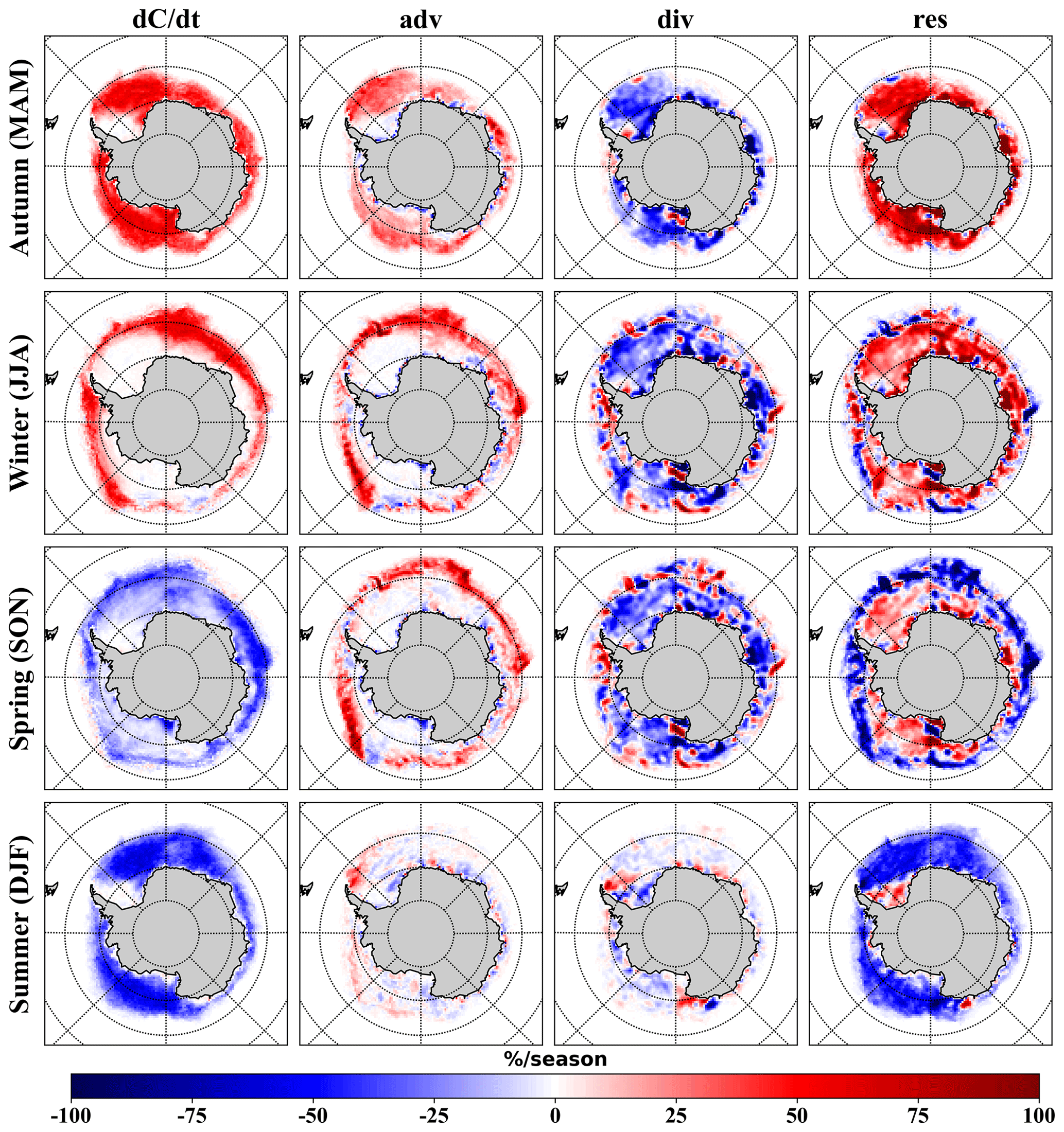
Figure B1 Seasonal mean of sea ice concentration (SIC) budget components for 2008–2017, calculated based on satellite-derived sea ice velocity (Kimura et al., 2013) and SIC (Meier et al., 2021) observations. The positive value stands for the SIC increase, and the negative value stands for the decrease.

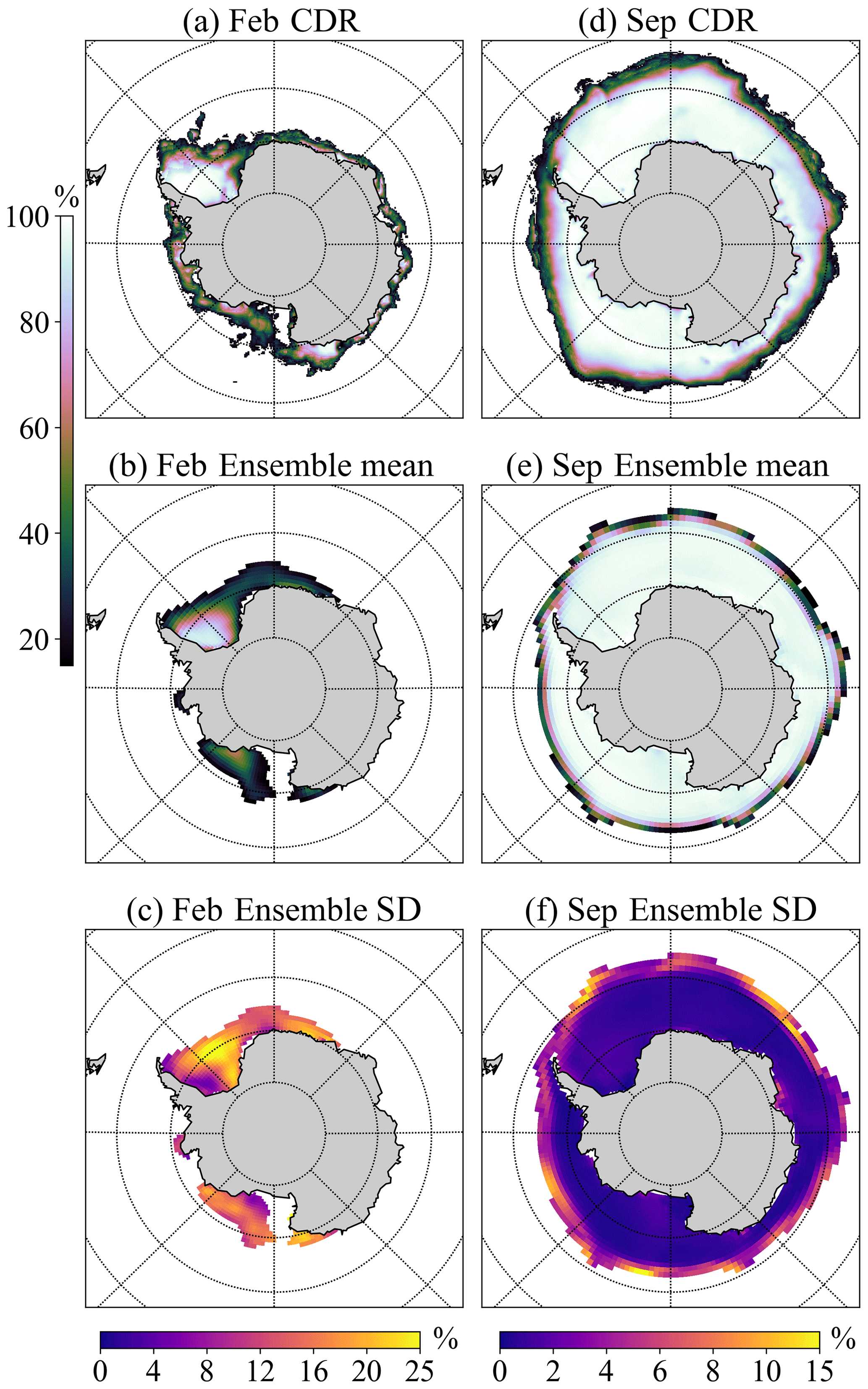
Figure B2 (a, b) Observed (NOAA/NSIDC Climate Data Record of Passive Microwave Sea Ice Concentration, version 4; CDR) and model ensemble mean February SIC climatologies (only SIC>15 % are shown). (c) Standard deviation of all model runs. (d–f) The same as (a–c) but for September.

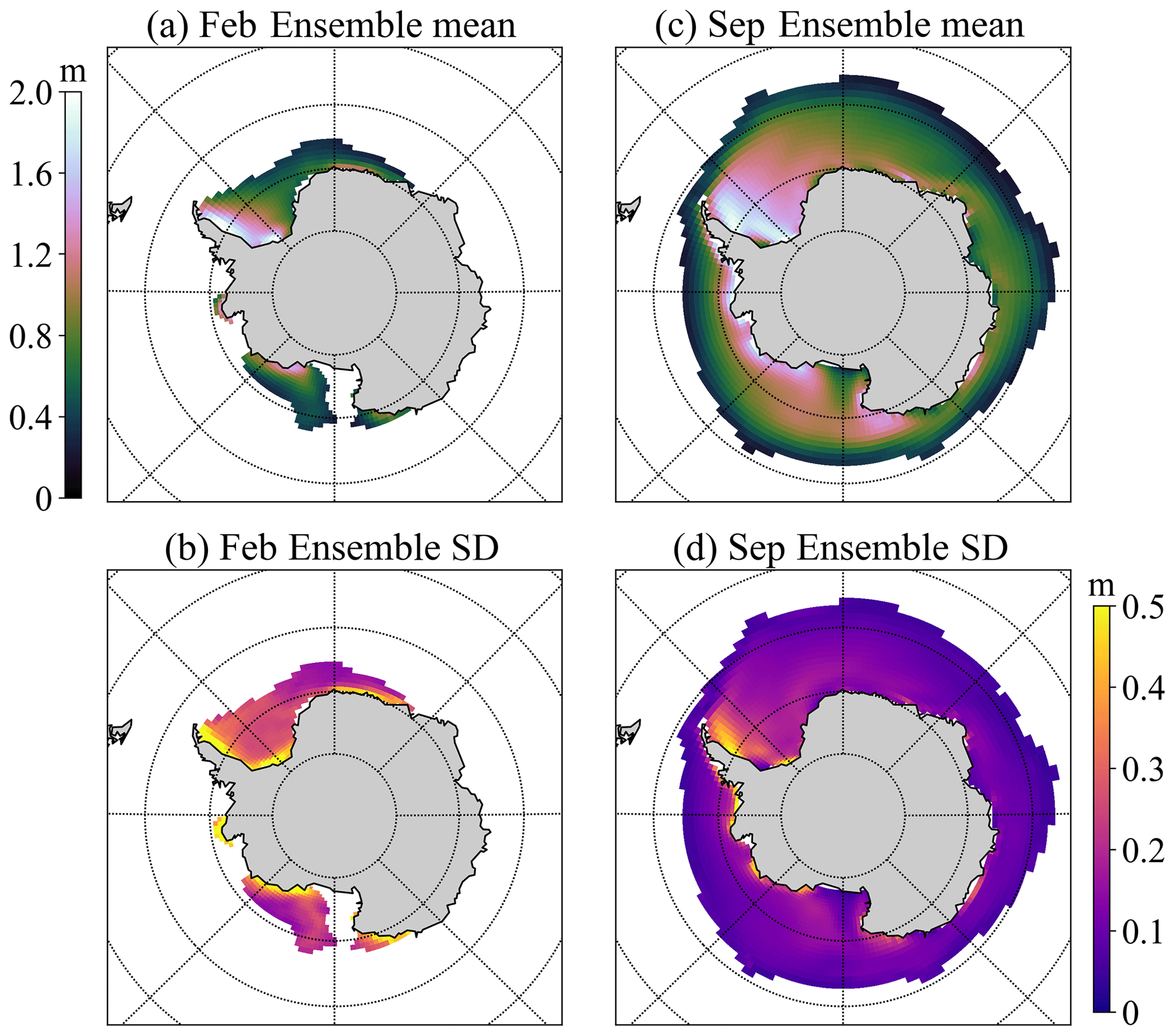
Figure B3 (a) Ensemble model mean February sea ice thickness climatologies (only SIC>15 % are shown) and (b) the standard deviation. (c, d) The same as (a, b) but for September.

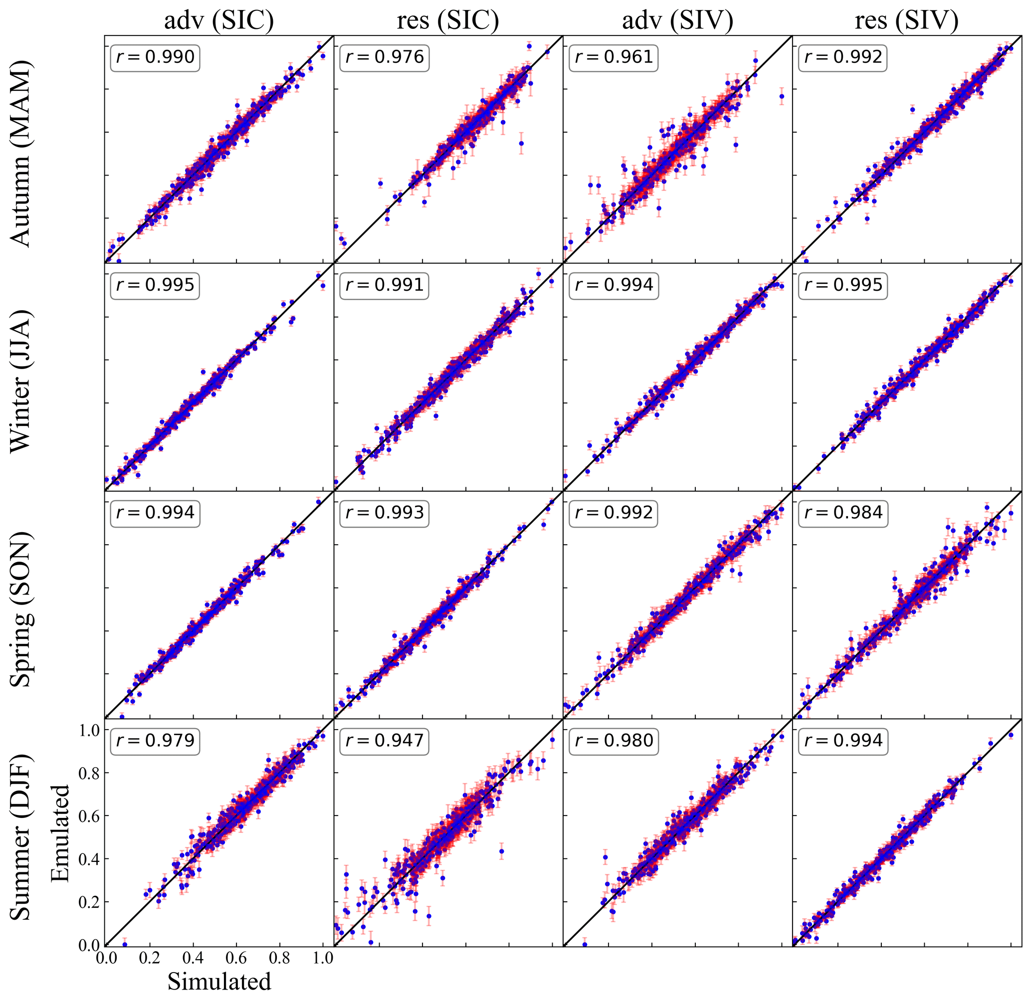
Figure B4 Validation results of the best Gaussian process (GP) emulators for each of the four metrics (area integrals of adv and res components in SIC and SIV budgets) selected by the 10-fold cross-validation. Each subplot consists of 449 error bars and a 1:1 line, and Pearson correlation coefficients are also listed. Each metric has been normalized (scaled to 0, 1 using the difference between the maximum and minimum values of the simulation) for better presentation.

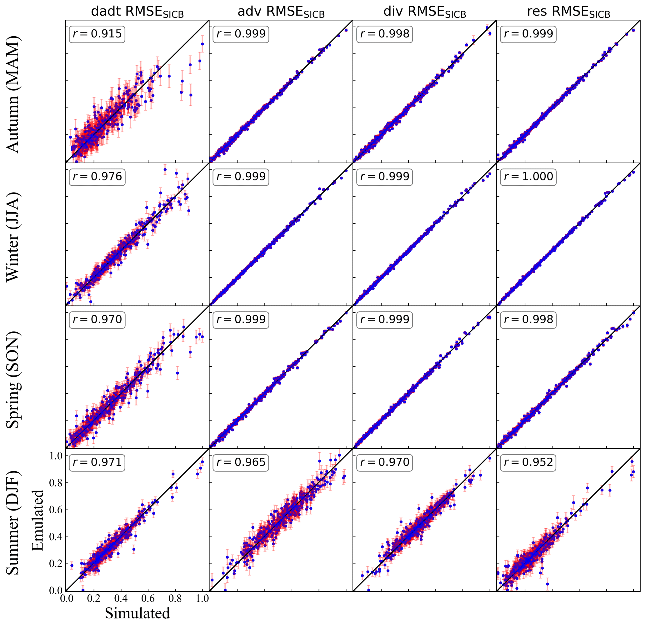
Figure B5 The same as Fig. B4 but for the root-mean-square error between SIC budget components of the simulation and the observation (RMSE_SICB).

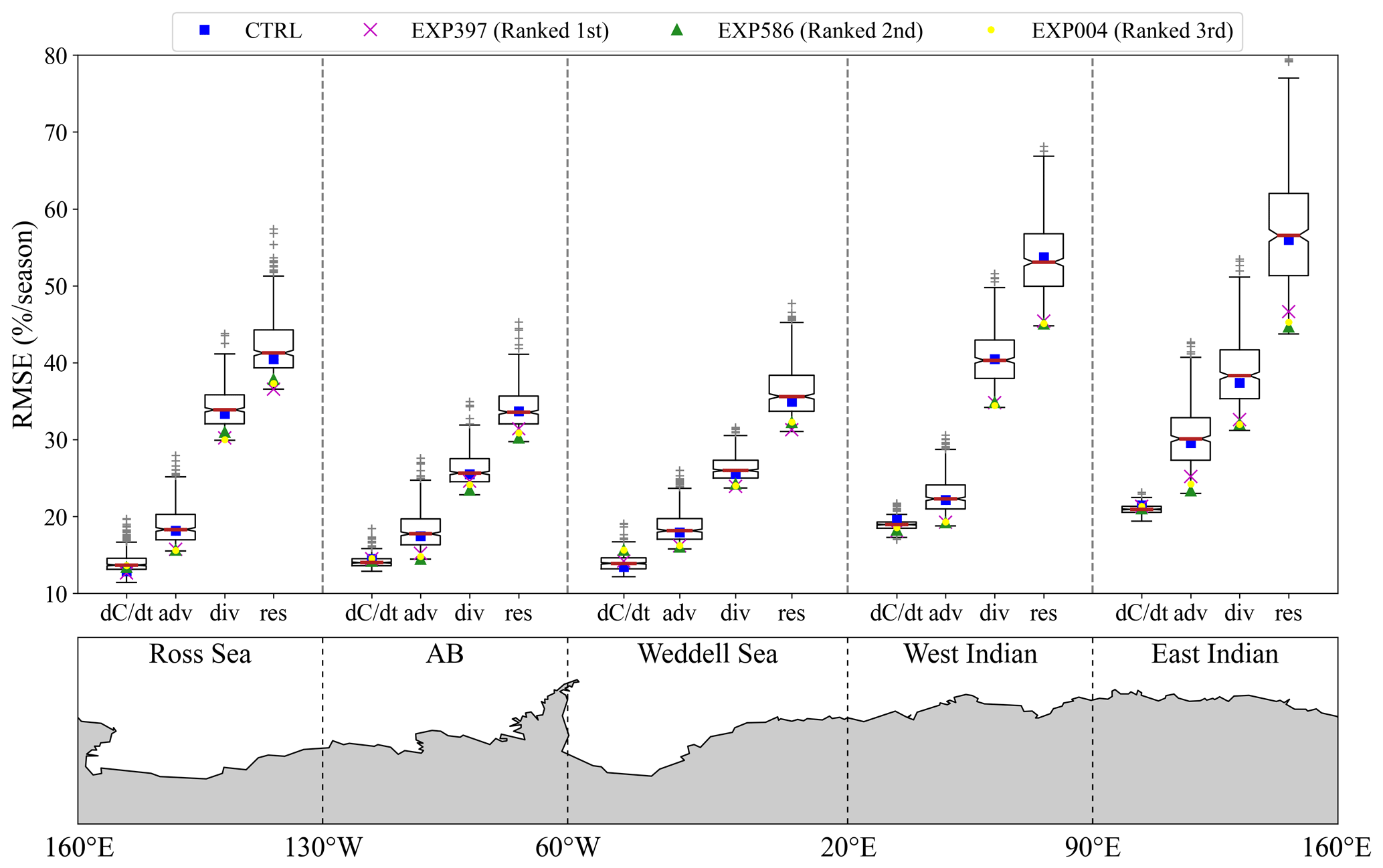
Figure B6 The same as Fig. 7, but the RMSE of each SIC budget term is averaged over four seasons and counted separately in each Southern Ocean sector. The dotted vertical line marks the demarcation of each sector. AB: Amundsen–Bellingshausen seas.

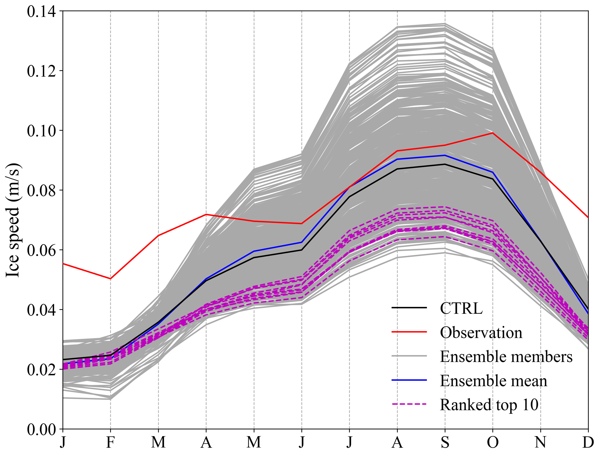
Figure B7 Sea ice speed seasonal cycles for the observation (Kimura et al., 2013) and simulations over 2008–2017. The simulated sea ice velocities are first interpolated onto the KIMURA data grid, then the spatial average of the ice speed is calculated in the areas where observations are available. The ice speeds of the 10 experiments with the closest SIC budget to the observation are marked with dashed magenta lines.

Figure B8 The same as Fig. 2a and b but for the Arctic.