the Creative Commons Attribution 4.0 License.
the Creative Commons Attribution 4.0 License.
 | 24 Feb 2023
Modeling large‐scale landform evolution with a stream power law for glacial erosion (OpenLEM v37): benchmarking experiments against a more process-based description of ice flow (iSOSIA v3.4.3)
Jörg Robl
Stefan Hergarten
David Lundbek Egholm
Kurt Stüwe
Following the tradition of modeling fluvial landscape evolution, a novel approach describing glacial erosion based on an empirical stream power law was proposed. This approach differs substantially from well-established process-based models applied to describe glacial erosion in mountain landscapes. Outstanding computational performance but a number of potential limitations compared to process-based models requires extensive testing to evaluate the applicability of this novel approach. In this study, we test the validity of the glacial stream power law and its implementation into a 2-D landform evolution model (OpenLEM) by benchmarking it against a state of the art surface process model based on the integrated second-order shallow-ice approximation (iSOSIA).
Despite completely different approaches, OpenLEM and iSOSIA predict similar ice flow patterns and erosion rates for a wide range of climatic conditions without re-adjusting a set of calibrated parameters. This parameter set is valid for full glacial conditions where the entire precipitation is converted to ice but also for an altitude-dependent glacier mass balance as characteristic for most glaciated mountain ranges on Earth.
In both models characteristic glacial features, such as overdeepenings, hanging valleys and steps at confluences emerge roughly at the same locations, resulting in a consistent altitude-dependent adjustment of channel slope and relief. Compared to iSOSIA, however, distinctly higher erosion rates occur in OpenLEM at valley flanks during the initial phase of the fluvial to glacial transition. This is mainly due to the simplified description of glacier width and ice surface in OpenLEM.
In this respect, we found that the glacial stream power approach cannot replace process-based models such as iSOSIA but is complementary to them by addressing research questions that could not previously be answered due to a lack of computational efficiency. The implementation of the glacial stream power law is primarily suitable for large-scale simulations investigating the evolution of mountain topography in the interplay of tectonics and climate. As coupling glacial and fluvial erosion with sediment transport shows nearly the same computational efficiency as its purely fluvial counterpart, mountain-range-scale simulations at high spatial resolution are not exclusively restricted to the fluvial domain anymore, and a series of exciting research questions can be addressed by this novel approach.
- Article
(20016 KB) - Full-text XML
- BibTeX
- EndNote


Glacial landforms, such as overdeepened valleys with U-shaped cross-sectional profiles, hanging valleys and bowl-shaped cirque valleys are common features throughout all mountain ranges with a distinct glacial imprint (e.g., Penck, 1905).
Their characteristic forms differ clearly from those of fluvially shaped mountains and represent some of the most consistent observations related to the interaction between glaciers and their beds (e.g., Anderson et al., 2006; Salcher et al., 2014). This enables the identification of climate impact on mountain topography via the prevailing erosional agent (i.e., glacier or river) through the analysis of landscape geometry. The quantification can be done with well-established topographic metrics, such as slope in longitudinal and cross-sectional profiles, valley curvature or local relief, and the dependence of these metrics on elevation (e.g., Egholm et al., 2009; Brocklehurst and Whipple, 2004; Pedersen et al., 2010; Prasicek et al., 2015; Sternai et al., 2011; Robl et al., 2015; Liebl et al., 2021; Salcher et al., 2021).
In the past, two completely different approaches were employed to describe the evolution of fluvial and glacial landscapes, respectively. Erosion rates of rivers were computed with the stream power law, which is a simple empirical relationship of geometrical properties of the drainage network (channel slope and catchment size) (Howard, 1994). Despite its simplicity, stream power incision models were extremely successful in explaining the evolution of topographic patterns over large temporal and spatial scales (e.g., Whipple and Tucker, 1999; Whipple, 2004; Wobus et al., 2006).
From the beginning of model development, glacial erosion models aimed at describing individual processes and their rates at the boundary layer between moving ice of the glacier and its bedrock (e.g., Braun et al., 1999; Egholm et al., 2011). While glacial landforms can be surveyed on a large scale after glacial retreat, the process of glacial erosion itself is elusive. Consequently, the complexity of glacial erosion is only poorly understood so far (e.g., Alley et al., 2019). However, during the last 2 decades, process-oriented landscape evolution models significantly contributed to determining the relationships between ice flow and different types of glacial erosion (e.g., plucking, abrasion).
Process-oriented models typically simulate the flow of ice over the considered topography and compute the erosion rate from the shear stress exerted to the bedrock. Since solving the full 3-D Stokes equations for the flow of ice over a complex topography is numerically expensive, a depth-averaged version – also known as the shallow-ice approximation (SIA) (Fowler and Larson, 1978; Hutter, 1980) – is implemented in 2-D landscape evolution models. This concept was inspired by models of fluvial erosion. The erosion rate is also derived from the shear stress exerted to the river bed here, and the SIA can be seen as a modified version of the shallow water approximation, which is widely used in modeling fluvial dynamics.
The model ICE-CASCADE (Braun et al., 1999) was the first 2-D landform evolution model based on the SIA. The integrated second-order shallow-ice approximation (iSOSIA) introduced by Egholm et al. (2011) additionally takes into account stresses arising from horizontal variations in flow velocity. This improvement is important to reproduce the characteristic cross-sectional shape of glacial valleys and enables the application to alpine topography with high topographic gradients. Furthermore, it overcomes the problem of deep and narrow gorges below the ice, which occurred in the original version of the SIA, in a physically reasonable way.
As a major challenge in modeling glacial erosion, the flow of ice consists of internal deformation and sliding along the bedrock. The sliding component is particularly relevant for erosion, but it is exposed to a high uncertainty since it also depends on the pressure of meltwater. Progress was made in this context by integrating models of glacier hydrology (Egholm et al., 2012; Herman et al., 2011) and recently by implementing more sophisticated models of subglacial erosion (e.g., Ugelvig et al., 2016, 2018). This facilitates the simulation of erosion on a sufficiently high level of detail to allow a direct comparison between the morphology of existing glacial landforms and those predicted by numerical models (e.g., Ugelvig et al., 2018; Egholm et al., 2017; Sternai et al., 2013; Liebl et al., 2021; Bernard et al., 2021). As a disadvantage, process-oriented models are still computationally expensive and face several limitations and stability issues when considering the mathematical and numerical complexity of ice dynamics and steep terrain. Furthermore, these models often include numerous parameters describing, e.g., the bedrock lithology, crack density, basal thermal conditions and water pressure fluctuations (Ugelvig et al., 2018; Leith et al., 2014; Egholm et al., 2017; Lai and Anders, 2021). These parameters are often difficult to constrain with field observations. Altogether, this limits the ability of this model type to describe the evolution of glacial topography at the mountain range scale.
Recently, a simplified concept for modeling the erosion of valley glaciers was proposed by Deal and Prasicek (2021). Not much later, a slightly different version of this concept was developed by Hergarten (2021a) and implemented in the landform evolution model OpenLEM. The concept is motivated by models of fluvial landform evolution at large scales, where rather simple models have been applied successfully. In contrast to more process-oriented models, these models do not simulate the flow of water and the resulting shear stress explicitly but use simple parameterizations of the erosion rate or the transport capacity along a river in terms of topographic properties.
The stream power incision model (SPIM) is the simplest model of this type. It implements the idea of detachment-limited erosion (Howard, 1994), which means that all particles entrained by the river are immediately swept out of the system. The SPIM predicts the long-term mean erosion rate E as a function of the channel slope S and the upstream catchment size A (a proxy for the long-term mean discharge) in the form
and involves only three parameters K, m and n. The stream power concept is not restricted to detachment-limited conditions. Kooi and Beaumont (1996) proposed a model describing transport-limited conditions, where the transport capacity was described in terms of channel slope and discharge. Since then, several formulations describing the general situation between the detachment-limited and transport-limited end-members were proposed (e.g, Whipple and Tucker, 2002; Davy and Lague, 2009; Hergarten, 2020). As such, models of the stream power type apparently provide a reasonable description of fluvial landform evolution at large scales without simulating the involved processes in detail.
The glacial stream power law proposed by Deal and Prasicek (2021) and Hergarten (2021a) proceeds from the more process-oriented models simulating ice flow and shear stress towards simple topography-based models. Formally, the expression for the erosion rate can even be written in the same form as the SPIM (Eq. 1), where the catchment size A has to be replaced by a proxy for the ice flux instead of the discharge, and the channel slope S must refer to the ice surface.
The implementation of the glacial stream power law in the landform evolution model OpenLEM (Hergarten, 2021a) offers a seamless combination with fluvial processes and an unprecedented numerical performance. Therefore, it could enable novel orogen-wide experiments on evolving topographic patterns under changing climatic conditions and examination of the relationship between Earth surface processes, crustal thickness, flexural isostatic uplift (Robl et al., 2020) and orographic precipitation (Hergarten and Robl, 2022). On the other hand, the glacial stream power law is exposed to a higher uncertainty than the fluvial version and has not yet been extensively tested. Furthermore, the implementation in OpenLEM required additional assumptions beyond the glacial stream power law. In contrast to rivers, glaciers are typically not much smaller than their valleys, meaning that their width and the rates of erosion across the valley have to be included in the model explicitly. In addition, the slope of the ice surface may differ strongly from the slope of the bed. Thus, replacing S in Eq. (1) with the slope of the bed is not a good approximation in contrast to the fluvial version. Hence, the implementation in OpenLEM required further assumptions, which may limit the applicability of the model to real-world scenarios.
Due to these assumptions, the question arises whether the glacial stream power law and the respective implementation in OpenLEM indeed open the doors towards large-scale simulations over long time spans or whether the simplifications cost too much of the complexity found in glacial landform evolution. In this study, we benchmark the implementation of the glacial stream power law against the state of the art ice flow model iSOSIA as a reference to get a clearer view under which conditions the simple model may be appropriate or could even compete with a more process-oriented models.
In this section, we briefly describe the theoretical principles, basic assumptions and peculiarities of the two employed models, focusing on the properties that are responsible for the major differences. Both landscape evolution models are able to simulate glacial, fluvial and hillslope erosion. However, benchmarking focuses on the fluvial to glacial landscape transformation, and hence the fluvial component is only considered to produce the initial landscape.
2.1 iSOSIA
The iSOSIA model describes the flow of ice and associated processes that eventually lead to erosion of the bed and, over long periods of time, to the formation of glacial landforms. The glacial mass balance is represented by the two-dimensional equation of continuity, which describes the change of ice thickness h through time according to
where qi is ice flux per unit width (m2 a−1) and div is the two-dimensional divergence operator. The rate of ice accumulation or ablation pi (m a−1) is simulated using a simple positive degree-day approach based on temperature and precipitation.
Glacier flow dynamics are computed by an integrated second-order shallow-ice approximation scheme (iSOSIA) (Egholm et al., 2011), where the relationship between ice deformation and stress is given by Glen's flow law
where
In these equations, and sij are the components of the strain rate tensor and the deviatoric stress tensor, respectively. Glen's flow law involves two parameters, where the factor AGlen depends on temperature and the exponent ψ≈3 (e.g., Cuffey and Paterson, 2010) describes the nonlinearity.
The combination of iSOSIA and Glen's flow law leads to depth-averaged horizontal velocities expressed as polynomials of the local ice thickness, which are solved iteratively due to velocity dependence (Egholm et al., 2011).
As a merit of the iSOSIA, variations in the shear stress exerted to the bed are resolved well (Braedstrup et al., 2016). This basal shear stress is an essential component of modeling glacial erosion. For temperate glaciers, however, sliding of the ice along the bed contributes much to the total velocity and even controls glacial erosion. Predicting the sliding velocity is more challenging than predicting the deformation velocity since it depends on glacial hydrology and on properties of the bed. The simplest model for subglacial sliding (Weertman, 1957; Budd et al., 1979) estimates the sliding velocity vs from the basal shear stress (ts) and the effective normal stress σe in the form
with the sliding coefficient Cw. To keep the model as simple as possible, we do not explicitly consider glacial hydrology here, but instead make the simple approximation that water pressure (which affects effective normal stress) is 80 % everywhere, as used in the earliest version of the iSOSIA model (e.g., Harbor, 1992; Egholm et al., 2011; Braun et al., 1999; Braedstrup et al., 2016).
In the original version of the iSOSIA model, erosion at the glacier base is solely driven by ice sliding:
The parameter Ka is an erosional coefficient, and l is an exponent describing the nonlinearity between erosion rate (E) and sliding velocity (vs). While this glacial erosion model is in principle only supported by the theory of glacial abrasion (Hallet, 1979), it also reproduces the patterns of glacial quarrying at least qualitatively, despite the fact that the influence of subglacial hydrology is strongly simplified (Egholm et al., 2012; Iverson, 2012; Ugelvig et al., 2016). Numerical simulations integrating a power law for quarrying (Ugelvig et al., 2016) and the effects of abrasive tools on glacial erosion (Ugelvig et al., 2018) show that the resulting landforms are qualitatively similar, regardless of the applied erosion law. Empirical data suggest that the value of l varies from to 2 and that Ka ranges from 10−7 to 10−4, depending on the choice of l (Herman et al., 2015; Cook et al., 2020; Koppes et al., 2015). All experiments are performed with l=1 and l=2 to explore the influence of nonlinearity in the erosion law (Eq. 12) on the pattern of glacial erosion and adjust the erosion constant Ka in order to result in fairly similar erosion rates for the different sliding exponents. Valley flank gradients tend to increase with duration of glacial occupation and progressive fluvial to glacial landscape transformation. While this landscape peculiarity is abundantly observed in nature, steep surface slopes strongly reduce the performance of the numerical model. First and foremost, hillslope erosion based on a nonlinear diffusion equation is implemented to efficiently remove material of steep valley flanks exceeding a pre-defined threshold slope, which can also be interpreted as some kind of landsliding in oversteepened terrain (e.g., Egholm et al., 2012; Roering et al., 1999). Practically, the model performance in accurately describing ice flow velocity and dynamics does not allow slopes exceeding 1 (45∘) and only a very simple landscape structure enables threshold slopes up to 2 (63∘). A detailed description of the iSOSIA model including highlights and limitations can be found in Egholm et al. (2011, 2012) and Braedstrup et al. (2016).
2.2 OpenLEM
The implementation of glacial erosion in OpenLEM is based on the glacial stream power law proposed by Deal and Prasicek (2021) and Hergarten (2021a). While OpenLEM also offers extensions towards sediment transport and fluvio-glacial processes, we only consider the simplest detachment-limited version here, where the glacial erosion rate is
This version involves only three parameters – the glacial erodibility Kg and the exponents m and n. The slope exponent n is identical to the exponent l in Eq. (6) used in iSOSIA.
In order to keep the formulation as close as possible to the fluvial stream power law, Hergarten (2021a) expressed the ice flux (volume per time) in terms of an equivalent catchment size Ai (area). For this purpose, the ice flux has to be divided by an arbitrary reference precipitation rate. The value of this reference precipitation rate is absorbed in the erodibility Kg, meaning that the erodibility implicitly carries information about the precipitation rate. Since Ai is still a measure of the ice flux and was only converted formally into an area, Eq. (7) is fully equivalent to the version proposed by Deal and Prasicek (2021).
In contrast to iSOSIA and to the glacial stream power law proposed by Deal and Prasicek (2021), the version implemented in OpenLEM assumes that the entire ice flux arises from sliding along the bed and neglects the contribution of deformation, which becomes increasingly relevant with increasing ice thickness (e.g., Cuffey and Paterson, 2010). At a given ice flux, neglecting deformation causes an overestimation of the sliding velocity and thus of the erosion rate (e.g., Deal and Prasicek, 2021; Prasicek et al., 2020a; Hergarten, 2021a). While neglecting deformation limits the applicability to thick glaciers, it turned out to be an advantage for simulating coupled fluvial and glacial systems. The ratio of the exponents m and n was found to be very close to the respective ratio for fluvial erosion by Hergarten (2021a), where typically 0.45 or 0.5 are used. As shown by Deal and Prasicek (2021), including deformation preserves the shape of Eq. (7) at least approximately but with a lower ratio . For simplicity, we use the default setting of OpenLEM with in all simulations.
As a fundamental difference towards models directly based on the SIA (Fig. 1a), the glacial stream power law uses the total ice flux instead of the flux per unit width. In order to implement this concept, OpenLEM considers dendritic networks where ice flows towards the neighbor with the steepest descent (D8 scheme, O'Callaghan and Mark, 1984), as widely used in fluvial landform evolution models. The glacial mass balance follows the steady-state version of Eq. (2), written in terms of fluxes (expressed as catchment size equivalents) for a discrete grid. This implies that glaciers are described by a single cardinal flow line in OpenLEM.
In contrast to rivers, however, including glaciers as linear objects in a 2-D landform evolution model is not useful. While rivers are typically much narrower than the width of their valleys and also narrower than the grid spacing of the model, this is not the case for glaciers. As a consequence, treating a glacier as a single-pixel line would underestimate the eroded volume and thus the sediment flux arising from glacial erosion. Therefore, OpenLEM uses an ad hoc approach for expanding glacial erosion over a wider area, which is illustrated in Fig. 1.
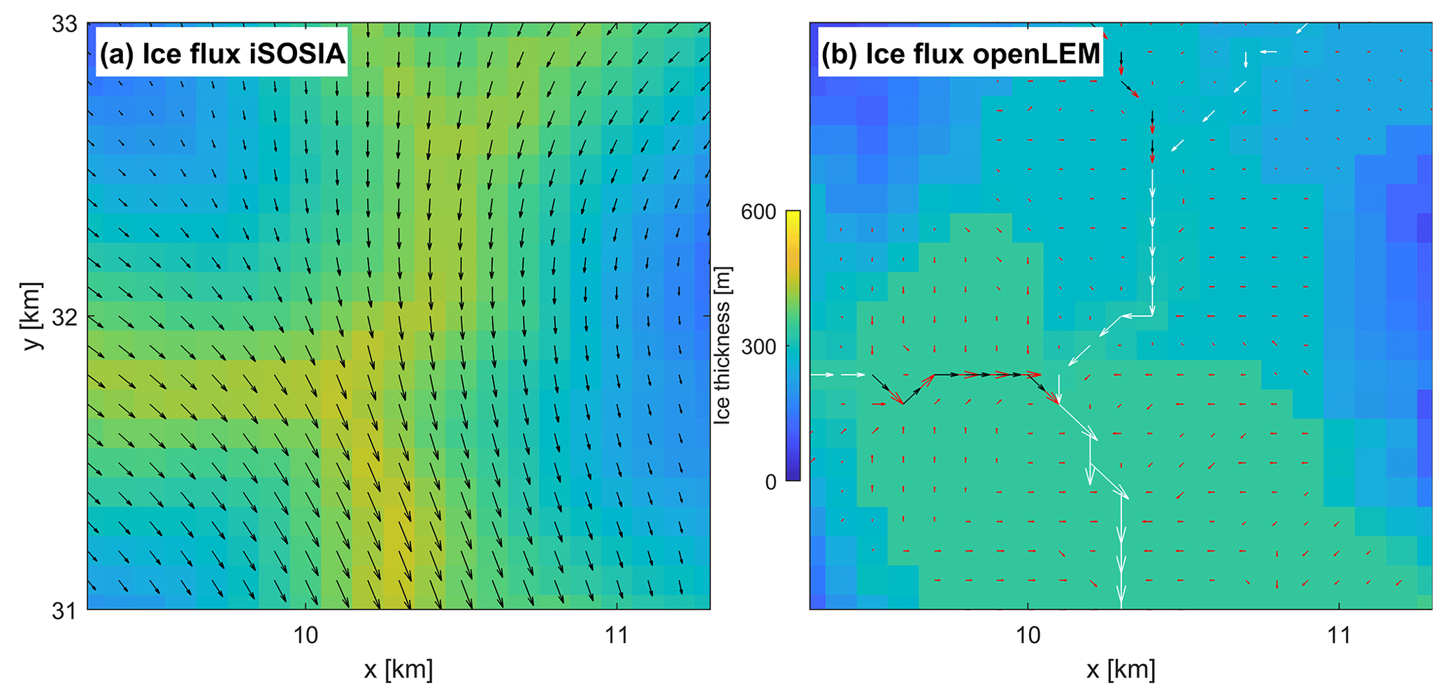
Figure 1Illustration of the different approaches to describe the ice flow pattern. (a) Ice fluxes per unit width in iSOSIA. (b) Ice fluxes in OpenLEM. Black and white arrows correspond to the ice flux obtained from the mass balance. Fluxes along the cardinal flow line are emphasized by white arrows. Red arrows are the artificially increased fluxes in a swath around the cardinal flow line, which are finally used in Eq. (7) for computing the erosion rate. The arrows are scaled arbitrarily in both parts. The domain corresponds to the red square in Fig. 2a and b.
In a first step, the cardinal flow line (white arrows in Fig. 1b) is extended to a swath of a given width w according to the empirical relation
with two parameters a and α, which was already used for developing the glacial stream power law. It is then assumed that the erosion rate of all points in the swath still follows Eq. (7) but with an artificially increased ice flux Ai derived from the respective value on the cardinal flow line (Fig. 1b – red arrows). This approach, which is the most complicated part of the implementation, is described in detail by Hergarten (2021a). It leads to a transition of V-shaped fluvial valleys to valleys with a rather flat floor, where some residual V-shape persists in order to avoid parallel flow patterns. Without going deeper into the details here, this ad hoc model for the across-valley shape is the most fundamental difference between the implementation in OpenLEM and in more process-oriented models such as iSOSIA.
In principle, OpenLEM could be used with zero ice thickness. This would mean that the slope S of the ice surface in Eq. (7) is identical to the channel slope at the bedrock. This simplification would, however, seriously affect the model's capabilities. In particular, the walls of glacial valleys would not be steeper than those of fluvial valleys. Since deriving the thickness h of the ice layer properly from a mass balance would cost most of the numerical efficiency, a constant thickness-to-width ratio
is assumed in OpenLEM. In other words, OpenLEM uses three parameters, a, α and δ, for characterizing the geometry of the ice layer. For the width-scaling exponent α, we use the value α=0.3 proposed by Hergarten (2021a) based on empirical data (e.g., Bahr, 1997; Prasicek et al., 2020b). In turn, the values of a and δ strongly depend on the initial valley geometries. Therefore, we perform several experiments in OpenLEM to estimate these parameters and find the best agreement with the landscape evolution produced by iSOSIA (see Sect. 3.1).
The rates of ice production and melting along the glacier have a strong influence on landform evolution (Pedersen and Egholm, 2013; Seguinot et al., 2018; Lai and Anders, 2021; Magrani et al., 2022). However, the implementation in OpenLEM by Hergarten (2021a) did not pay much attention to a realistic description of these rates since focus was on the formulation and the implementation of the glacial stream power law. It was assumed that these rates only depend on the actual elevation Hi of the ice surface (implicitly via the surface temperature). A simple linear approach with a cutoff was used,
where p is the total precipitation rate and pi is the rate of ice production (pi>0) or melting (pi<0). This rate is zero at the equilibrium line altitude (ELA) He, while the entire precipitation is converted into ice above a given elevation Hf.
While this approximation is not fundamentally different from the approach used in iSOSIA above the ELA, melting below the ELA turned out to be more critical. The recent version of OpenLEM offers two options here. In the original version (Hergarten, 2021a), Eq. (10) was simply continued to elevations Hi<He, i.e., to negative rates of ice production. However, making this approach compatible with the description of glaciers by a cardinal flow line requires allowing negative ice fluxes. Otherwise, melting would practically act only on the cardinal flow line instead of the entire surface of the glacier. The alternative concept allows for defining an arbitrary function for the melting rate along the cardinal flow line. In order to obtain the total volume of melting ice per time and glacier length, this rate is multiplied by the width of the glacier according to Eq. (8). Both concepts of describing the rate of melting will be tested against the model implemented in iSOSIA in Sect. 3.2.
Our work aims to assist potential users in selecting the ideal model for the specific issue they are trying to solve. Therefore, we are performing a series of experiments that ensure balanced benchmarking between OpenLEM and iSOSIA. While the two models compared in this study start from basically the same equations, the approximations made are so different that they finally lead to totally different differential equations. In its simplest form, the implementation in OpenLEM uses a single equation for the erosion rate as a function of the topography and the ice flux instead of a coupled system of equations for the ice surface, the flow velocities and the erosion rate. As an immediate consequence, OpenLEM involves highly lumped parameters, such as the glacial erodibility, which combine parameters related to different processes. A central question is whether these lumped parameters can be calibrated with respect to a given parameter set of iSOSIA. In the best case, the calibration should not be restricted to an individual example but valid for a large range of scenarios.
As a challenge beyond the different model parameters, both models were designed for applications on different scales. While the flow of ice and glacial erosion are the key components of iSOSIA, the glacial component of OpenLEM was developed as an extension of a fluvial model with a focus on large-scale simulations over millions of years. Hence, the benchmarking scenarios have to be designed carefully. For the first set of experiments, we use a synthetic initial topography that has already been used in a benchmark study of iSOSIA against the full-Stokes Elmer/Ice model (Braedstrup et al., 2016), as well as in studies on the impact of subglacial quarrying (Ugelvig et al., 2016), subglacial sediment transport (Ugelvig et al., 2018) and contrasting climatic forcing (Magrani et al., 2022) on glacial erosion. This topography represents a synthetic mountain topography based on the detachment-limited version of the stream power incision law for fluvial conditions. It does not contain any glacial landform elements, and its valleys have V-shaped cross sections and graded longitudinal river profiles with steep headwaters and decreasing channel slopes in the downstream direction. The model domain is 20×40 km and consists of 200×400 cells at a spatial resolution of 100 m. This system size allows for simulations with iSOSIA at a moderate computing effort. While 100 m is also a typical resolution for OpenLEM, this model allows for simulating much larger domains, e.g., 5000×5000 nodes (see examples of Hergarten, 2021a).
In order to distinguish differences between the two models arising from the erosion model from differences owing to the glacial mass balance, the first set of experiments was conducted on two levels. At the first level (Sect. 3.1), fully glaciated conditions are considered, where the entire precipitation is converted into ice, and melting is disregarded. This scenario provides insights into the differences between the two erosion models but poses some technical challenges. While the simplified treatment of the ice flux in OpenLEM allows for open boundary conditions where ice can leave the domain, iSOSIA assumes closed boundaries by default. However, it is possible to operate both models with zero ice thickness at the downward boundary, which means that we assume an instantaneous melting of the entire ice immediately at the boundary. Such a scenario is not necessarily realistic, but it ensures the same boundary conditions for both models and also provides insights into the evolution of overdeepenings in both models.
At the second level, a glacial mass balance is introduced (Sect. 3.2). This can be seen as a minimum scenario of glacial erosion at given climatic conditions. Both models for melting available in OpenLEM (Sect. 2.2) are tested here, where the key question is whether the calibrated parameters can be adopted from the fully glaciated scenario or a recalibration is required. Finding that a recalibration is necessary would seriously limit the applicability of OpenLEM since we would probably also need a recalibration if the climatic conditions change. The first series of experiments is concluded by a short investigation of the effect of nonlinearity in the erosion law (Sect. 3.3).
The next experiment (Sect. 3.4) proceeds in a direction further away from what OpenLEM was designed for. Using a simpler topography with a single valley, the conversion from a V-shaped fluvial cross section to a U-shaped glacial cross section is investigated in detail. Reproducing U-shaped valleys without further assumptions was one of the major achievements of the second-order shallow-ice equations introduced in iSOSIA compared to the original shallow-ice approximation. In turn, OpenLEM relies completely on an ad hoc assumption that the glacial stream power erosion law (Eq. 7) holds for the entire glacier with a modified ice flux.
The final experiment (Sect. 3.5) is not a direct comparison of the two models. Here we will consider long-term landform evolution of an entire mountain range over several glacial cycles. Such simulations are still not feasible at a reasonable computing effort with iSOSIA. Therefore, this experiment illustrates what kind of simulations are possible if we accept the limitations of OpenLEM found in the previous experiments.
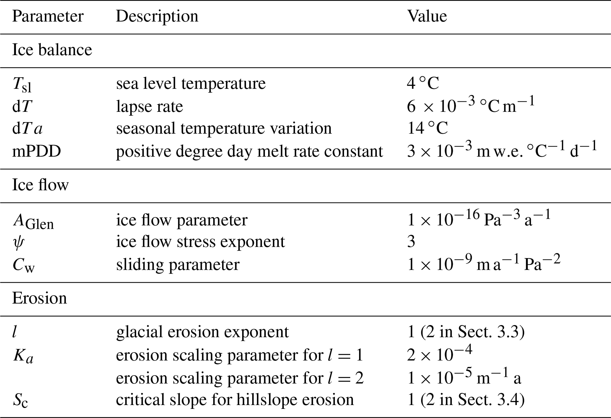
Since the model parameters of iSOSIA are related more closely to the involved processes than those of OpenLEM, we define parameter values for iSOSIA (Table 1) based on the experience from previous studies (Egholm et al., 2012; Pedersen and Egholm, 2013; Braedstrup et al., 2016; Ugelvig et al., 2016; Liebl et al., 2021; Magrani et al., 2022). The parameter values required in OpenLEM are then calibrated.
3.1 Experiment 1.1: fully glaciated conditions
Full glacial conditions with a spatially and temporally uniform ice production rate represent the simplest benchmarking experiment because the feedback between erosion, area above the ELA and ice flux is avoided. While changes in topography affect the ice flux locally, the large-scale flow pattern is not affected much in such a setup. In particular, the total ice flux through a cross section of a large valley only depends on the (constant) rate of ice production and on the catchment size, meaning that it does not change much through time and is also similar in both models.
For this scenario, OpenLEM involves only three parameters beyond the rate of ice production, where we assume 0.1 m a−1. These are the glacial erodibility Kg (Eq. 7), the factor a in Eq. (8)m which defines the glacier width, and the ratio of thickness and width δ (Eq. 9). In principle, the respective equations additionally contain the exponents m and α. However, these are constrained better by real-world data, meaning that we do not consider them adjustable parameters and used the default values m=0.5 and α=0.3.
The glacial erodibility was adjusted to Kg=19 Ma−1, based on the criterion that the cumulative eroded volume after 100 ka of glacial occupation is the same in both models (Fig. 3a). The two other parameters, which define the width and the thickness of the glacier, were adjusted more visually. The factor a in Eq. (8) was set to 1.5 in nondimensional coordinates (digital elevation model, DEM, pixels). This means that a glacier with an ice flux equivalent to the ice production of 1 pixel at a given reference production rate has a width of 1.5 pixels. In all of our simulations, we assume a reference precipitation (and thus also reference ice production rate) of 1 m a−1 (so that the nondimensional ice production rate is 0.1 in this simulation). Therefore, the choice a=1.5 means that an ice flux of 104 m3a−1 generates a glacier width of 150 m (a=150 m0.4). For the thickness-to-width ratio (δ in Eq. 9), the default value of 0.25 from Hergarten (2021a) was adopted. These parameter values will be used in all subsequent simulations, meaning that further calibration will only relate to the influence of the climatic conditions.
3.1.1 Ice configuration
The simulations were performed over a time span of 100 kyr. Figure 2 illustrates the ice configuration in an early phase of the transformation (t=4 ka) and at the end of the simulation (t=100 ka). The choice of t=4 ka instead of the initial situation takes into account that iSOSIA builds up the ice cover gradually, whereas OpenLEM assumes an instantaneous adjustment.
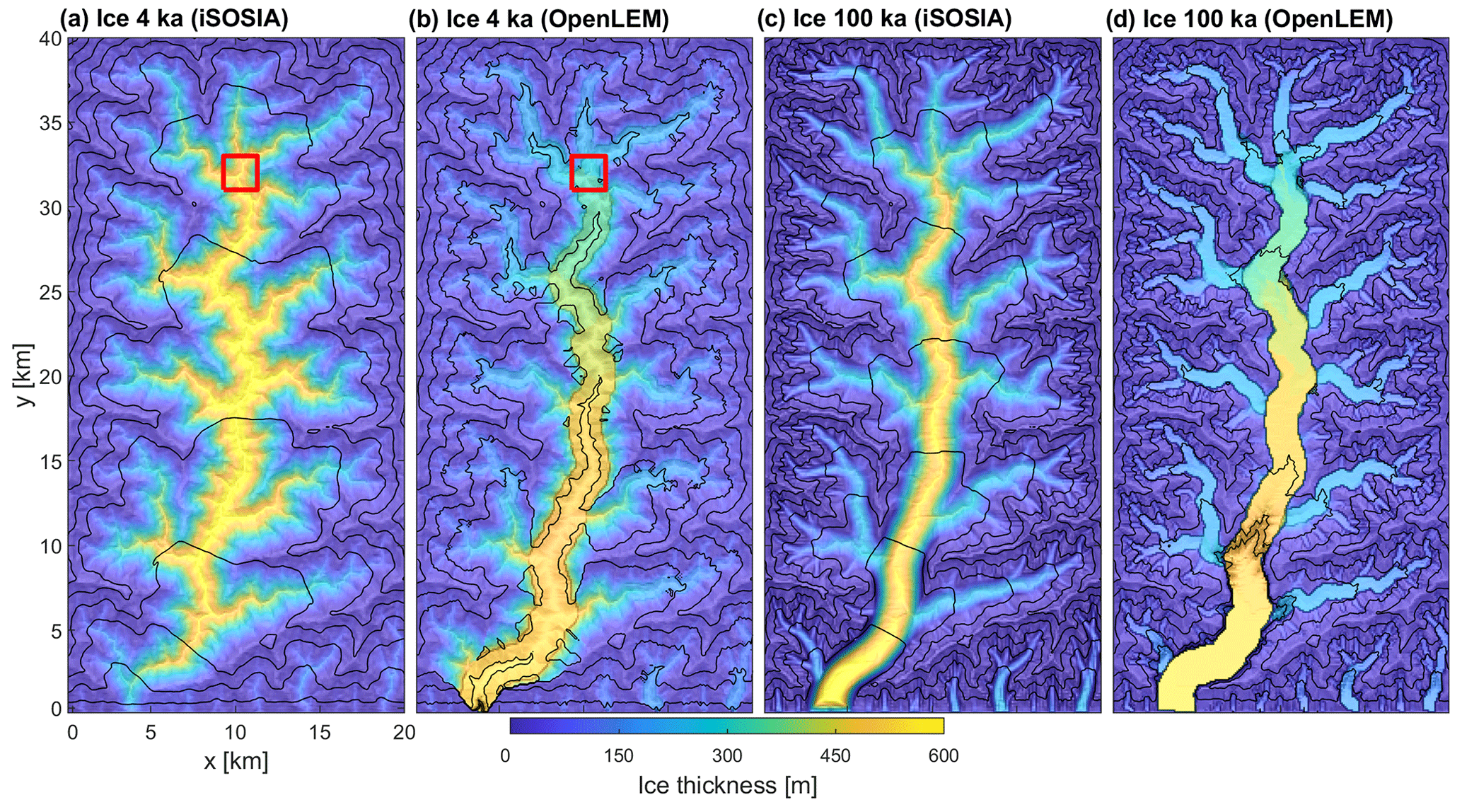
Figure 2Differences in ice configuration in the numerical experiments with a constant ice production rate of 0.1 m a−1. (a, b) Ice thickness after 4 ka and (c, d) after 100 ka for iSOSIA and OpenLEM (δ=0.25, a=150 m0.4), respectively. Spacing of contour lines is 200 m. The red square in (a) and (b) depicts the domain of Fig.1.
The ice configurations show clear deviations between the models, owing to the different complexity in describing the distribution of the ice over the topography. OpenLEM expands the glacier to a swath centered on the cardinal flow line and assumes a more or less constant ice thickness across the valley (Fig. 2b). Starting from a steep V-shaped fluvial valley, the resulting ice configuration is obviously unrealistic. However, the ice configurations of both models become increasingly similar with increasing time of glacial occupation and the corresponding transition to U-shaped glacial valleys (Fig. 2c, d). By widening and flattening the valley floors, glaciers of a predefined width fit better into their valleys, and the initially large gradients of the ice surface in OpenLEM disappear.
3.1.2 Altitude-dependent erosion over time
As shown in Fig. 3, the deviations in the ice configuration go along with differences in erosion rates. These are strongest in the early phase of the simulation. For clarity, the erosion rates of both models were not compared on a point-by-point basis but integrated over four distinct elevation slices (Fig. 3c). The slices were derived from the initial topography (without ice) and kept throughout the simulation in order to avoid a feedback of the erosion rate on the definition of the slices.
OpenLEM predicts significantly higher erosion rates in the two lowest elevation slices (H≤1000 m) at the onset of landscape transformation than iSOSIA (Fig. 3b). In the beginning, OpenLEM predicts considerably higher erosion rates than iSOSIA at elevations below 1000 m, (green lines in Fig. 3b). However, the difference vanishes or is even reverted partly after about 25 ka. The increased erosion rates in OpenLEM at the onset of glacial occupation are related to the rapid adjustment of V- to U-shaped valley cross sections, particularly at the trunk glacier.
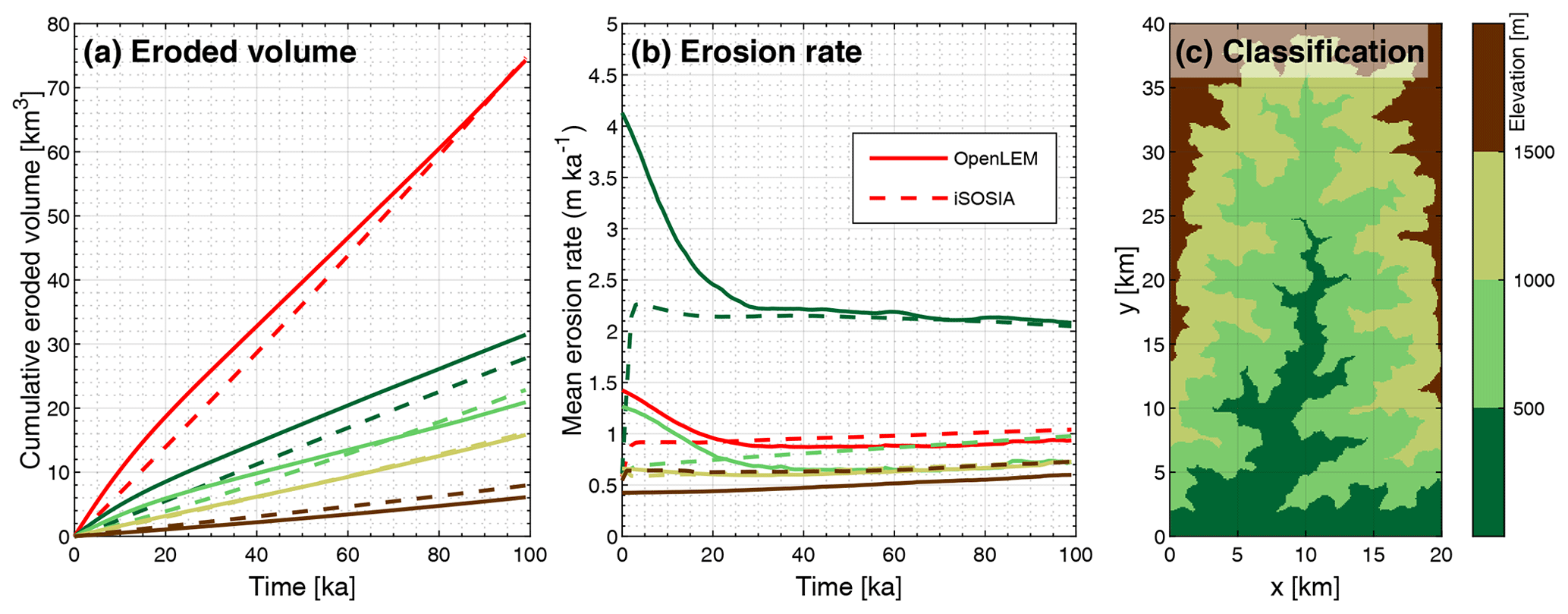
Figure 3Differences and similarities in the erosion history as computed by iSOSIA and OpenLEM (shown as dashed and solid lines, respectively). (a) Cumulative eroded volume and (b) mean erosion rate of the entire landscape (red lines) and the rising elevation ranges as shown in (c).
While the erosion rates still decrease slowly in the lowermost elevation range after the initial adjustment has taken place, they increase continuously in the higher ranges. This trend is consistent in both models, but a systematic shift between the models is found. OpenLEM increasingly underestimates the erosion rates with increasing elevation compared to iSOSIA. This difference is not immediately related to the distribution of the ice, but rather to neglecting the contribution of deformation to the ice flux in OpenLEM as discussed in Sect. 2.2. If the ice flux is given, neglecting deformation causes an overestimation of the sliding velocity and thus of the erosion rate. Since deformation becomes more relevant with increasing thickness (e.g., Cuffey and Paterson, 2010), the erosion rates are overestimated at low elevations, where the trunk glacier becomes thick. By focusing on the total eroded volume in the calibration of the erodibility Kg, we shifted the overestimation at low elevations towards an underestimation at high elevations.
3.1.3 Propagation of knickpoints
Setting the southern boundary cells to an ice thickness of zero (technically required in iSOSIA) generates a strong gradient in the ice surface. Since erosion is driven by the gradient of the ice surface in both models, the bedrock is rapidly eroded until the ice surface has flattened. This results in the formation of a strong overdeepening with a depth controlled by the initial ice thickness. While this overdeepening expands progressively upstream in both models, shape and evolution of the longitudinal profiles are different (Fig. 4). The glacial stream power law implemented in OpenLEM leads to an advection equation, which generates distinct knickpoints moving upstream as widely observed for fluvial erosion (e.g., Royden and Perron, 2013; Hergarten, 2021b). Downstream of the knickpoint, a flat valley floor and ice surface emerges, which impedes further erosion (Fig. 4). In turn, the shallow-ice equations contain a strong diffusion component since the flow velocity depends on the actual slope of the ice surface. This diffusive component keeps both the ice surface and the velocity field smooth. Taking into account horizontal stresses in the second-order approximation implemented in iSOSIA strengthens this effect further. Since the sliding velocity is the primary control on the erosion rate, the smoothness is transferred to some degree to the topography. As a result, the overdeepened region expands upstream without generating a distinct step in elevation. Only a break in slope can be observed in the early phase, but this discontinuity fades through time.
In our example, the difference between the advective behavior of the glacial stream power model used in OpenLEM and the more diffusive shallow-ice equations implemented in iSOSIA is emphasized by the artificial boundary condition. The difference may become relevant in real-world applications if rapid changes in the climatic conditions occur. OpenLEM may exaggerate the effect of such changes on the topography. Noting that transport-limited fluvial erosion models also show a rather diffusive behavior (Hergarten, 2021b), one may be tempted to switch from the detachment-limited erosion model to a transport-limited model for glacial erosion. While OpenLEM would allow this option, we should be careful not to generate a coincidence of the results for the wrong reason.
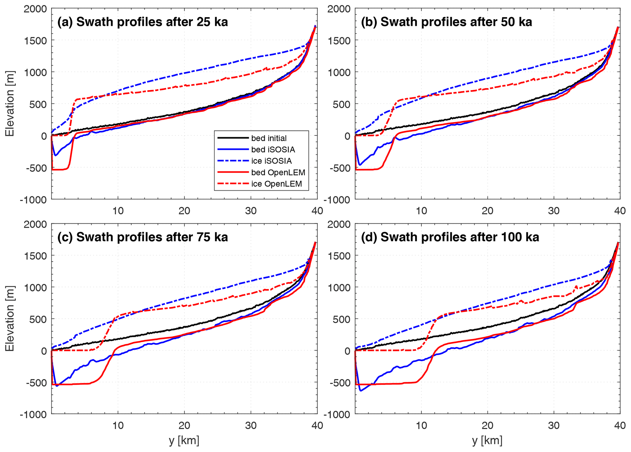
Figure 4Topographic evolution of an initially fluvial landscape (Fig. 2) subject to glacial erosion. (a–d) The minimum elevations of the longitudinal swath profiles (across the entire landscape) in the iSOSIA and OpenLEM experiments are shown as blue and red lines, respectively. The corresponding ice surface is shown as a dashed line.
Apart from the differences in the evolution of the receding valley floor, similar erosion patterns emerge in both models. However, we observe a slightly less pronounced valley incision in the lower part and a slightly stronger incision in the upper part in OpenLEM compared to iSOSIA (Fig. 4).
3.2 Experiment 1.2: simulations with glacial mass balance
In the previous section, a reasonable agreement of the ice configurations and the erosion rates was achieved by adjusting the erodibility Kg and the geometry factors a and δ for fully glaciated conditions (except for the initial phase). As discussed in Sect. 3, however, glacial landform evolution is very sensitive to the glacial mass balance (ice production and melting). The next step is to test whether the simple approach used in OpenLEM works sufficiently well under predefined climatic conditions where the surface is only partly covered with ice.
In order to focus on the differences between the two models, factors such as orographic effects on precipitation, snow avalanches and exposure to the sun are not considered, although they exert some influence on the glacier mass balance in alpine valleys. However, these are more external influences that could be included in both models. As a further simplification, we kept the climatic conditions constant in order to enforce a continuous fluvial to glacial landscape transformation. This allows a direct comparison of process rates and emerging landforms over the entire time span of the benchmark simulations without considering transient climatic effects.
3.2.1 Ice mass balance models and ice configuration
For the parameter values listed in Table 1 and a uniform precipitation rate of 1 m a−1, the positive degree-day (PDD) model used in iSOSIA predicts an ELA of around 1330 m. Precipitation is entirely converted into ice above an elevation of about 1830 m, which is called the full ice altitude (FIA) in the following. These two elevations are the same as He and Hf in the simple linear glacial mass balance of OpenLEM (Eq. 10) and thus define the calibration for this model. While the simple linear mixing approach agrees well with the more elaborate approach used in iSOSIA between the ELA and the FIA, Fig. 5a reveals that extrapolating the linear relation below the ELA – the default approach in OpenLEM (gray lines) – increasingly underestimates the melt rate with decreasing elevation.
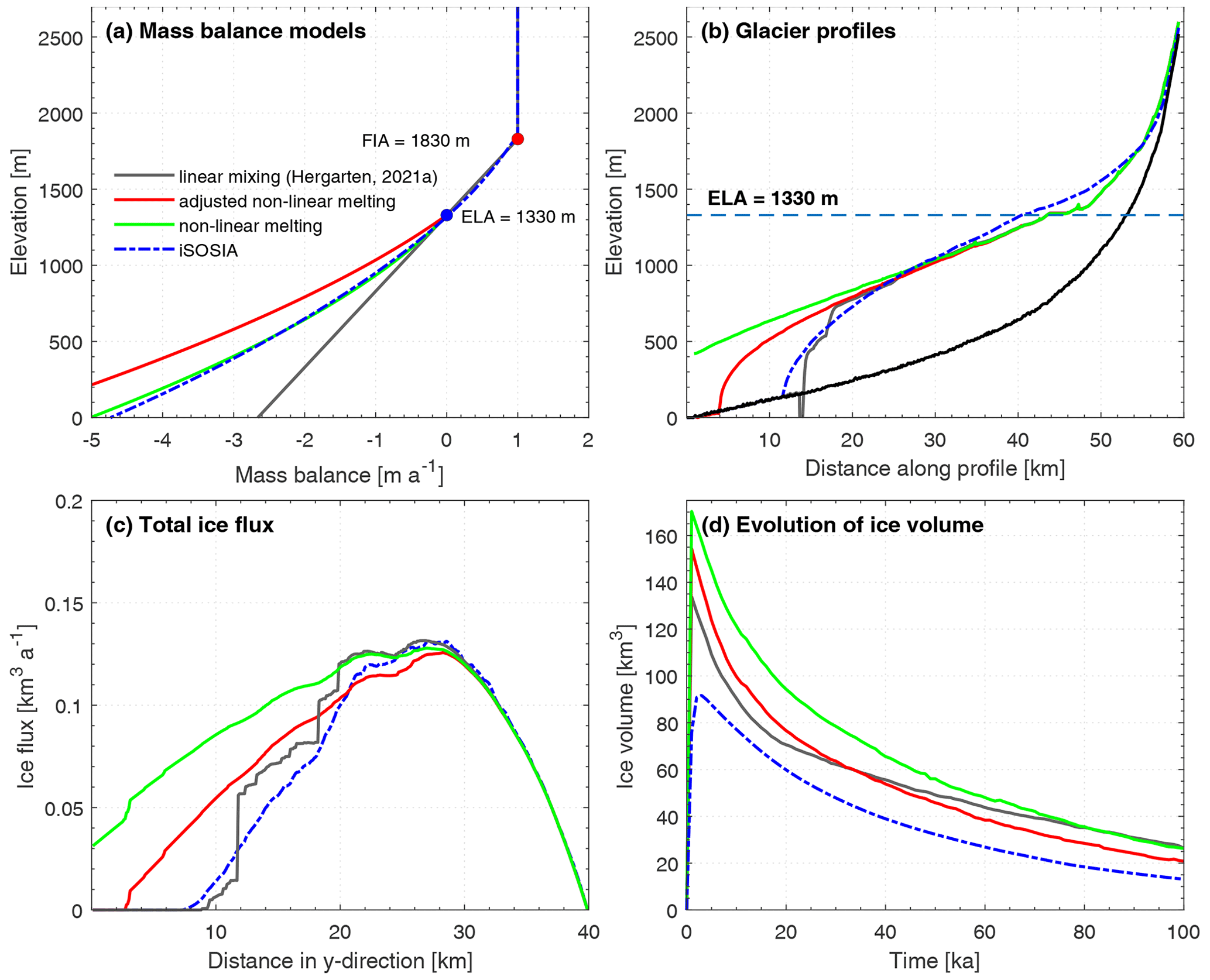
Figure 5Comparing the ice mass balance models. (a) Different altitude-dependent mass balance models for iSOSIA (dashed blue line) and OpenLEM (solid lines). Impact of the mass balance models on (b) ice thickness along the cardinal flow line, (c) total ice flux in the y direction and (d) total ice volume. Note that (b) and (c) represent the ice configuration after 4 ka, which coincides with the time of the maximum ice volume of iSOSIA.
Despite the underestimation of the melt rate, the initial longitudinal glacier profile and the respective ice fluxes agree surprisingly well between OpenLEM and the prediction of iSOSIA (Fig. 5b, c). However, this approach generates steep gradients in the ice surface and a sharp drop in ice flux. This effect is directly related to the implementation in OpenLEM, where confluences with tributaries that include large areas below the ELA cause a rapid melting of the glacier. As already visible in the results of Hergarten (2021a), these steep gradients cause a rapid, localized incision and thus an irregular pattern of overdeepenings. This effect is already visible at t=4 ka in Fig. 5b. Apart from this probably unrealistic behavior, we should be careful with the simple default approach implemented in OpenLEM since the origin of the rapid melting at the glacier terminus is so different in both models that the apparently good agreement is probably coincidental.
Therefore, we also tested the option to introduce a custom function to describe melting of ice in OpenLEM. As shown in Fig. 5a (green line), extending the linearly extrapolated rate by a quadratic term in the form
provides a reasonable approximation down to quite low elevations. However, it is immediately recognized in Fig. 5b, c that melting is then too slow. This discrepancy is related to the treatment of the glacier width. The implementation in OpenLEM concentrates the total volume of melting ice to the cardinal flow line by multiplying the melt rate (Eq. 11) by the glacier width (Eq. 8). However, the width scaling factor a in Eq. (8) was adjusted in Sect. 3.1 mainly with regard to the overall erosion rate and not to replicate the exact ice surface. In Fig. 2, it looks as if the glacier was wider in OpenLEM than in iSOSIA, but this impression arises from the region with a thick ice cover. Owing to the different cross-sectional shapes, the ice surface is even wider in iSOSIA, particularly in the early phase. To counteract this, we adjusted the total melting rate of OpenLEM by a factor of 1.5 (Fig. 5a – red line), which leads to a better agreement with the results of iSOSIA regarding the longitudinal glacier profile and the ice flux (Fig. 5b, c).
In general, all experiments show the same trend, with ice volume quickly reaching its maximum value and decreasing with duration of glacial occupation (Fig. 5d). This trend is a direct effect of reducing the elevation by glacial erosion. However, the different mass balance models result in distinctly different initial and evolving ice volumes. Owing to the simple parameterization of the glacier width, all OpenLEM scenarios predict a considerably higher ice volume than iSOSIA, particularly during the first phase where the topography is still dominated by V-shaped fluvial valleys. However, the rapid transformation of the valley cross section causes the ice volume to decrease more rapidly than in iSOSIA. For the scenario with the adjusted melt rate and the increased effective width (red curve), the difference towards the iSOSIA simulation approaches a rather constant value of about 12 km3 quite quickly. This residual extra volume can be attributed to the different shape of the final valley, which is rather rectangular in OpenLEM and rather parabolic in iSOSIA.
While Fig. 6 confirms the overall similarity of the ice configurations of both models, we observe some deviations by comparing the results in detail. In the early phase (Fig. 6a, b), OpenLEM not only predicts a longer downstream extension of the main glacier but also a stronger filling of tributary valleys with ice, although these valleys receive little ice from their upstream catchment. In reality, this effect occurs as soon as the ice surface in the trunk valley is higher than the valley floor of the tributaries. In iSOSIA, this upstream flux of ice is modeled dynamically (following the actual ice surface) and also reduces the ice flux of the trunk glacier. In turn, OpenLEM uses a steady-state mass balance and simply fills up the tributaries with a horizontal ice surface, meaning that the flux into tributary valleys is zero. While the effect on erosion in tributary valleys is small in both models, it makes a difference concerning the mass balance, which is partly responsible for the longer extension of the glacier in OpenLEM.
As a second difference, the trunk glacier retreats somewhat faster in OpenLEM than in iSOSIA (Fig. 6c, d). Therefore, the ice volume remaining after 100 ka is more concentrated in wide valleys with a rather flat floor, and the larger ice volume compared to iSOSIA (Fig. 5d) does not correspond to a larger area covered by ice.

Figure 6Differences in ice configuration in the numerical experiments with a elevation-dependent ice production rate (ELA = 1330 m). (a, b) Ice thickness after 4 ka and (c, d) after 100 ka for iSOSIA and OpenLEM (δ=0.25, a=150 m0.4). The spacing of the contour lines is 200 m. The 1330 m contour line is highlighted in white. The path of the cross-sectional and glacier-long profiles depicted in Figs. 5 and 9 are shown as a dashed and continuous red line, respectively.
Overall, adopting the nonlinear increase in melt rate at low elevations (Eq. 10) and assuming a wider ice surface than the glacier width parameterized by Eq. (8) appears to be a viable way to make the glacial mass balance of OpenLEM consistent with that of iSOSIA. Revisiting Fig. 5, the scaling factor of 1.5 by which we increased the width artificially for computing the melt rate may even look too large. However, we must keep in mind that OpenLEM is not a model for simulating ice patterns on a surface, but landform evolution. Therefore, the choice of the scaling factor was not only based on the results shown in Fig. 5 but also on the results concerning erosion discussed in the following.
3.2.2 Altitude-dependent erosion over time
Figure 7 provides the analysis of the erosion rates and the cumulative eroded volume for the elevation ranges defined in Fig. 3c. As the most striking difference towards the fully glaciated scenario, the ranking of the domains has changed. While the lower ranges experienced the highest erosion rates under fully glaciated conditions, this applies to the highest regions now since the ice flux decreases with decreasing elevation below the ELA. Due to the decrease in elevation by erosion, the two lowermost regions (green curves) are even deglaciated at the end of the simulation, meaning that glacial erosion ceases.
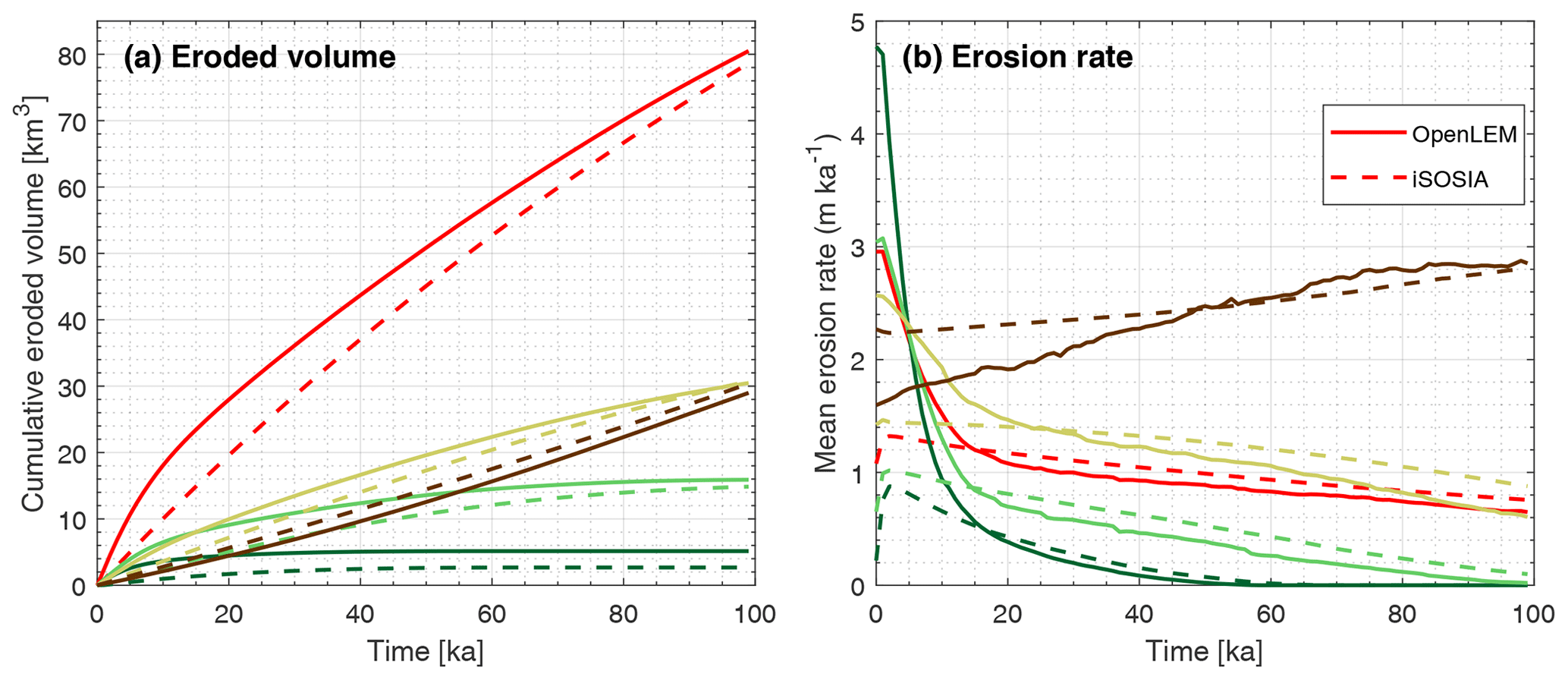
Figure 7Differences and similarities in the erosion history as computed by iSOSIA (dashed lines) and OpenLEM (solid lines). (a) Cumulative eroded volume and (b) mean erosion rate of the entire landscape (red lines) and the rising elevation ranges as shown in Fig. 3c.
Similar to the fully glaciated scenario, OpenLEM predicts considerably higher erosion rates than iSOSIA during the early phase of the simulation, owing to the rapid adjustment of V- to U-shaped valley cross sections. The deviation in the early erosion rates is particularly strong in the lowest range (dark region). Here the deviation mainly arises from the greater initial extent of the glacier predicted by OpenLEM in combination with a faster retreat. An opposite effect is observed in the uppermost range (brown curve). Also similar to the fully glaciated scenario, OpenLEM starts with lower erosion rates than iSOSIA here. However, the effect vanishes through time here, while it persisted in the fully glaciated scenario. After about 20 ka, the erosion rates of the other elevation slices do not differ much between the two models. The cumulative volumes over the entire simulation even agree quite well since the lower rates predicted by OpenLEM for t⪆20 ka compensate the higher rates of the early phase. A considerable difference only persists for the lowermost region, where the erosion predicted by OpenLEM is very strong initially and ceases quite quickly.
Both models show that glacial erosion primarily modifies the landscape along the initial fluvial drainage lines, while the ridges and steep hillslopes are less affected. Besides similarities in the evolution of large-scale topographic patterns, Fig. 8 reveals some differences in the erosion patterns. In iSOSIA, erosion is focused at the steep headwaters and along the main valley trunk, progressively removing interlocking spurs of the initially fluvial landscape. This results in an erosion pattern with many local maxima at an early stage of landscape transformation. Over long times, the removal of the interlocking spurs leads to a distinct valley straightening and widening (Fig. 8a). In OpenLEM, glacial erosion is initially concentrated at the valley flanks (Fig. 8b), where both local slope and ice thickness are high. As a consequence of the initial phase of rapid valley widening and flattening, local slope and ice thickness across the valley become uniform, which in turn results in uniform valley incision rates. At a late stage of glacial landscape formation, the erosion patterns of both models become similar, with major differences occurring only locally at some valley flanks (Fig. 8d–f). When comparing the final landscapes of both models, the main valley of the OpenLEM simulation appears much wider. This is mainly due to the geometry of the valley flanks, which are almost vertical in OpenLEM and hardly steeper than 45∘ in iSOSIA.

Figure 8Model-dependent evolution of erosion patterns. Glacial erosion computed by (a) OpenLEM and (b) iSOSIA and (c) differences in erosion between the two models over the first 10 ka of glacial occupation. Panels (d), (e) and (f) show the same properties but for the time slice between 90 and 100 ka. Contour spacing for surface elevation is 200 m.
3.2.3 Evolution of longitudinal and cross-sectional profiles
While the results of Sect. 3.2.2 suggest that the adjusted nonlinear model for the melt rate (Eq. 10) is not only a reasonable approach for the glacial mass balance but also approximates the large-scale erosion pattern predicted by iSOSIA quite well, we now focus on the specific differences between the two models using various topographic metrics.
A transverse profile at y=27.5 km is chosen to highlight the spatial variations of the glacial erosion pattern at different times and parts of the landscape (Fig. 9). While the valley is widened and lowered simultaneously in the experiment of iSOSIA (blue lines), the widening in OpenLEM (red lines) takes place entirely during the first 25 ka, followed by solely vertical incision afterwards. As the glacier retreats, the ice flux becomes smaller and the valley floor narrower. With a total incision of about 350 m predicted by iSOSIA, the deepest point of the valley floor is finally about 30 m lower than predicted by OpenLEM. The discrepancy between the two models in erosion amounts is less than 10 %. The width of the resulting glacial trough – measured at the valley shoulder – is fairly similar, but the geometry is distinctly different in both models (Figs. 8d, e, 9).
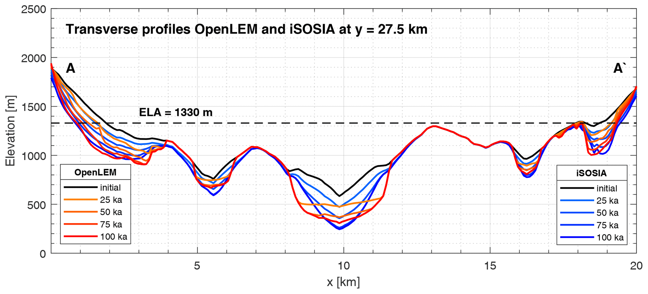
Figure 9Time series of the evolution of the transverse profiles in the OpenLEM and iSOSIA experiment shown as red and blue lines, respectively. The position of the cross section is depicted in Fig. 6.
Changes in the long profile are shown by a time series of a catchment-wide swath profile (Fig. 10). Both models consistently describe the large-scale topographic pattern of a fluvial to glacial landscape transformation. This includes several hundred meters of erosion at the trunk valley and distinctly lower erosion at the nearby ridgelines. In combination, this results in an increase in valley relief and also applies to the formation of very steep headwalls at the uppermost reach of the trunk valley. Deviations between the models occur only at small-scale topographic features. While the length profile of OpenLEM (red line) remains largely smooth during glacial excavation, the iSOSIA profile is punctuated by many differently sized steps, which are related to the formation of small overdeepenings whenever tributaries enter the main valley (Fig. 10, blue line).
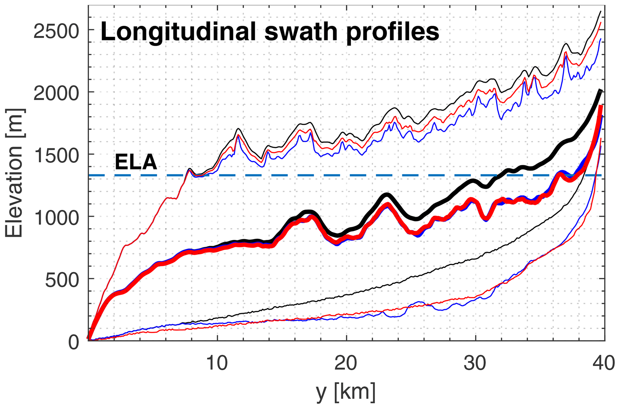
Figure 10Topographic evolution of an initially fluvial landscape subject to glacial erosion. Maximum, mean and minimum elevations of longitudinal swath profiles of the initial (black) and final landscapes in the iSOSIA and OpenLEM experiment are shown as blue and red lines, respectively.
3.2.4 Altitudinal distribution of slope, relief and erosion
The altitudinal distribution of channel slope, local relief and total erosion is sensitive to glacial imprint and allows the quantification of the glacial impact on fluvial topography. The distribution of channel slope versus surface elevation has been applied to characterize both fluvial and glacial terrain (Hergarten et al., 2010; Kühni and Pfiffner, 2001; Robl et al., 2015; Liebl et al., 2021). Channel slopes in the direction of steepest descent are calculated for each cell and for cells with a threshold flow accumulation area of 1 km2 by a standard single-flow algorithm (D8) implemented in Topotoolbox (Schwanghart and Kuhn, 2010; Schwanghart and Scherler, 2014). Local relief is computed by subtracting the minimum from the maximum topography within a sliding window with a radius of 1000 m.
The initial topography is characterized by a channel slope–elevation distribution with a narrow interquartile range at all elevations and maximum slopes below 0.4. Taking a subset with catchment sizes larger than 1 km2, mean channel slopes are in general smaller but show the same altitudinal trend (Fig.11a, b – blue lines). As soon as glacial erosion starts reshaping the fluvial topography, the mean and interquartile range of the slope increases above an altitude of 800 m in both models. This trend amplifies with ongoing glacial occupation (see supplementary videos – video02-OpenLEM and video02-iSOSIA; https://doi.org/10.5281/zenodo.6557805), and after 100 ka the topography shows a slope maximum between 2000 and 2400 m (Fig. 11a, b). The shape of the resulting slope–elevation distributions of both models is quite similar. However, the topography resulting from the OpenLEM simulation features a greater increase in mean channel slope with elevation compared to iSOSIA, as well as a larger spread between the first and third slope quartiles (Fig. 11a, b – error bars).
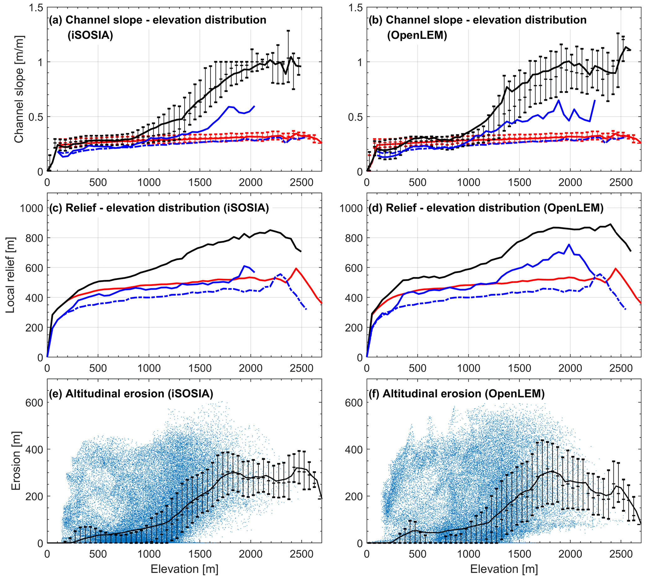
Figure 11Altitudinal changes in topography. Panels (a) and (b) show channel slope–elevation distributions of iSOSIA and OpenLEM and (c) and (d) present local relief–elevation distributions with local relief as the difference of maximum and minimum elevation within a sliding window with a radius of 1000 m. Solid red and black lines represent mean values for the original fluvial and the resulting glacial landscape, respectively. Thin bars show the interquartile range. Solid (glacial landscape) and dashed (original landscape) blue lines show mean values representing the drainage system (A>1 km2). Mean values and the interquartile range of all plots are derived from elevation bins with a bin size of 50 m. (e, f) Altitudinal correlation of erosion. Each blue dot represents the cumulative erosion of a single cell. Black lines indicate the mean accumulated erosion, and black bars represent the interquartile range for the respective elevation slice.
These deviations among the two models represent differences in the valley geometries with flat floors and very steep flanks in OpenLEM and smooth rounded glacial troughs getting continuously steeper from the valley floors towards the flanks in iSOSIA. This is, on the one hand, due to the different approaches to describe glacial erosion (i.e., governed by the flow of ice in iSOSIA and parameterized in OpenLEM) but, on the other hand, also due to technical limitations of iSOSIA handling steep landforms, where slopes greater 1 lead to a dramatic decrease in numerical efficiency and ultimately to numerical instability. Defining a threshold slope of 1 avoids such technical issues but causes steep topography (i.e., valley flanks) to decay quickly by mass diffusion. As a result, iSOSIA loses the ability to form largely vertical valley flanks, landforms that are, however, characteristic of most iconic glacial landscapes on Earth.
As qualitatively shown in valley-long and cross-sectional profiles, spatial variations in the glacial erosion pattern change the local relief from the original fluvial to the resulting glacial landscapes. The original topography shows a strong increase in mean relief at low elevations up to 400 m followed by a slow steady increase up to an altitude of about 2400 m. At the highest elevations, mean relief drops (Fig. 11c, d – red lines). In both models, 100 ka of glacial erosion causes a similar increase in local relief compared to the initial landscape at all elevation levels, with the highest increase being from mid-altitudes to high altitudes (Fig. 11c, d – black and blue lines). Again, the small differences between the models are due to model-dependent differences in valley geometry.
The altitudinal correlation of erosion is consistent with changes in relief and channel slope–elevation distributions (Fig. 11e, f). Up to an elevation of 1200 m, mean cumulative erosion increases slightly but does not exceed 100 m in both models. Mean cumulative erosion strongly increases above the ELA (1330 m) with maximum values exceeding 250 m at mid-altitudes (1800 m). At high elevations, erosion in iSOSIA remains consistently high, while in OpenLEM it decreases continuously toward the summit region. While the mean cumulative erosion is similar in both models, the spread between the first and third quartiles is larger in OpenLEM. We observe a clear trend that the iSOSIA model is more erosive at the highest elevations.
3.3 Experiment 1.3: nonlinear erosion law
As discussed in Sect. 2.1, the uncertainty in describing glacial erosion quantitatively even concerns the exponent l in Eq. (6). Therefore, we also tested the value suggested by Herman et al. (2015) and Koppes et al. (2015), which means that the erosion rate increases quadratically with the sliding velocity instead of linearly. We kept all parameter values of both models except for the factors Ka (iSOSIA) and Kg (OpenLEM). These factors were adjusted in such a way that the total volume eroded over 100 kyr is close to that of the respective linear model. For iSOSIA, we set the erosion constant Ka to 10−5 m−1 a instead of . The ratio of these two values, 20 ma−1, tells us that the erosion is stronger for l=2 than for l=1 at sliding velocities above 20 m a−1 and vice versa. For OpenLEM, we used Kg=24 instead of Kg=19 Ma−1.
The respective erosion patterns are shown in Fig. 12. While the large-scale patterns are not affected strongly by the choice , distinct differences occur along the large glaciers. The erosion predicted by iSOSIA becomes more heterogeneous, with several patches where more than 500 m are eroded. These occur preferably at inside bends of the valley. Consequently, iSOSIA makes the valleys more straight in map view and thus shorter for l=2, while the course of the valleys is governed by the initial cardinal flow line in OpenLEM under all conditions.
Flattening of the valley floor takes places even faster for n=2 in OpenLEM, although it was already faster than in iSOSIA for n=1. In turn, the erosion along the cardinal flow line decreases and is finally much weaker than in iSOSIA. This difference in the long profiles may be more relevant than the patches of strong erosion, which are mainly a horizontal shift of the valleys.
Overall, it must be pointed out that the differences between the two considered models increase if a nonlinear erosion law is used, although the discrepancies in the large-scale erosion patterns still seem to not be crucial.

Figure 12Differences in the evolving erosion pattern with n and l=1 or 2 of OpenLEM and iSOSIA. Erosion is measured over a time span of 100 kyr. Contour spacing is 100 m.
3.4 Experiment 2: V to U shape conversion
The geometry of glacial valleys with their characteristic U-shaped cross sections represents one of the most striking features of glacial erosion in mountain landscapes. Here we test OpenLEM's ability to gradually form glacial valley cross sections and compare the rates of transformation from a fluvial to a glacial geometry to those of iSOSIA. Experiments were conducted with different precipitation rates to investigate how the resulting valley width increases with ice flux. To isolate the effect of valley widening and deepening as function of ice flux, we use a simple topographic structure mimicking a single fluvial valley with a concave longitudinal profile and a V-shaped cross-sectional form (Fig. 13). The valley structure and its elevation is given by
where ΔH=2250 m and R=750 m are the relief in the longitudinal and transverse direction, respectively. The valley features a length of L = 40 km and width of W=4 km. The exponent b is set to 0.5 and controls the concavity of the longitudinal profile. The application of the best fit parameters for the glacier mass balance and the scaling of glacier width and ice thickness as determined in Sect. 3.1 and 3.2 results in glacier fronts, which align fairly well in both models in the considered range in precipitation rates from p=0.1 to 1 m a−1. To study the continuous evolution of glacial valley cross sections, we choose a cross-sectional profile at the upper reach (at y=6 km). This guarantees a continual ice flow over the entire duration of the simulation for all investigated precipitation rates. Although glacial erosion gradually lowers the contributing area upstream from the cross section, the ice surface area remains entirely above the ELA, causing an fairly constant ice flux over the duration of glacial erosion.
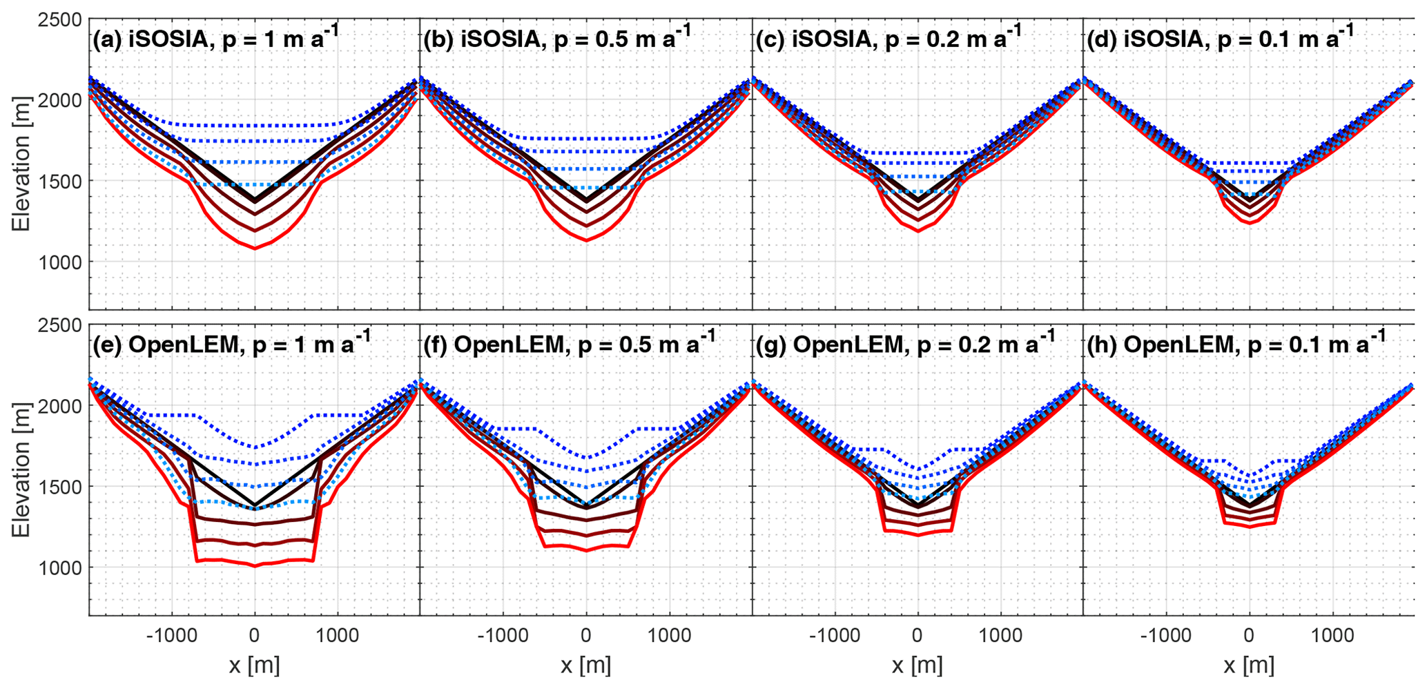
Figure 13Evolution of cross sections as a function of precipitation rate (p=1, 0.5, 0.2 and 0.1) for (a–d) iSOSIA and (e–h) OpenLEM. The black line is the initial profile. The four red lines are after 5, 25, 50 and 75 ka. The lines turn from black to red with time. The ice surfaces are shown for the same time steps as dashed blue lines.
In both models, erosion is focused at the valley flanks, resulting in a wide, flat-bottomed trough with steep sides (Fig. 13). Valley widening and valley deepening scale consistently in both models with the precipitation rate and hence the ice flux. However, the resulting geometry of the trough and the rates of adaptation to this geometry differ between the two models.
In iSOSIA, we observe a continuous glacial transformation with a smooth, low-gradient ice surface and a valley that grows with a fairly steady pace in width and depth. This results in rounded, parabolic cross sections (Fig. 13a–d). The initial ice surface in OpenLEM parallels the bedrock topography due to laterally extending the ice thickness of the cardinal flow line (uppermost dashed blue line in Fig. 13e, f). Hence, the ice surface shows large gradients at the valley flanks. In combination with the same ice thickness as along the cardinal flow line, this leads to high erosion rates and as a consequence to a rapid widening of the valley floor (uppermost red line in Fig. 13e, f). The shape of the valley and of the ice surface adjusts as long as the transverse slope is considerably larger than the longitudinal slope of the cardinal flow line. Compared to iSOSIA, this leads to a significantly faster transformation from the original V-shaped valley towards a valley with a fairly flat floor confined by almost vertical flanks.
Apart from the valley geometry, the rates of erosion observed at the center of the valley agree well in both models. At a precipitation rate of p=1 m a−1, OpenLEM predicts an approximately 20 % higher erosion rate compared to iSOSIA throughout the simulation period. The difference decreases towards dry conditions and vanishes for p=0.1 m a−1. As discussed in Sect. 3.1.2, OpenLEM tends to overestimate erosion rates for thick glaciers since ice deformation is neglected.
Despite the model-specific differences in valley geometry, the resulting valley widths agree quite well in both models. In OpenLEM, the valley width measured at the base of the glacier trough decreases from about 1.5 km for p=1 m a−1 to 0.75 km for p=0.1 m a−1 (lowermost red lines in Fig. 13e, f). Owing to the almost vertical walls, the width increases by less than 100 m from the bottom to the valley shoulder. The scaling of the glacier width p is an immediate consequence of the parameterization of the width by the ice flux in OpenLEM. Using the default value α=0.3 for the exponent in Eq. (8), the width becomes proportional to p0.3. Then 1 decade in p changes the width by a factor of 100.3=2, as observed above.
Due to its parabolic shape, the glacial trough emerging in iSOSIA increases in width from the valley floor towards the valley shoulder. Measured at the valley shoulder, however, the valley width of iSOSIA and OpenLEM simulations agree almost perfectly.
The results of this section confirm that the parameterization of the glacier width and the calibration of the erodibility holds for a considerable range in ice fluxes. At large ice fluxes, neglecting the deformation of ice leads to a moderate overestimation of the erosion at the center. As the most important difference, the cross-sectional shape of the valleys differ strongly, and the final shape is approached in OpenLEM much faster than in iSOSIA.
3.5 Experiment 3: the next step – large-scale simulations over several glacial cycles
In our third experiment, we take advantage of the superior computational performance of OpenLEM by performing a mountain-range-wide simulation over several cycles of glaciation, which would be hardly solvable by iSOSIA due to the high computational effort.
For understanding such a coupled fluvial–glacial system and its potential imprint in the present-day topography, transport and deposition of sediments are particularly relevant. OpenLEM is not limited to fluvial and glacial incision but is also able to simulate sediment transport at almost the same numerical efficiency. Sediment transport is implemented in OpenLEM in the form of the shared stream power model, which was introduced by Hergarten (2020) and discussed in detail by Hergarten (2021b). It is a generic model based on the idea that the stream power term AmSn (Eq. 1) is used jointly by erosion and sediment transport in the form
where Q is the sediment flux (volume per time). In contrast to the SPIM (Eq. 1), which uses a single parameter for the erodibility, the shared stream power model involves two parameters Kd and Kt with the same physical units, where Kd describes the ability to erode the bedrock and Kt the ability to transport sediment. The shared stream power model is used here in the most recent version proposed by Hergarten (2022). This version switches to a fully transport-limited model, characterized by Kd→∞, at sites where sediment is deposited in order to avoid an artificially long transport range in combination with low rates of deposition.
We adopt the parameter values Kd=6.5 Ma−1 and Kt=4.1 Ma−1 used by Hergarten and Robl (2022). While OpenLEM can also simulate glacial sediment transport using the shared stream power model, we stay at the detachment-limited version with Kg=19 Ma−1 used in the previous experiments.
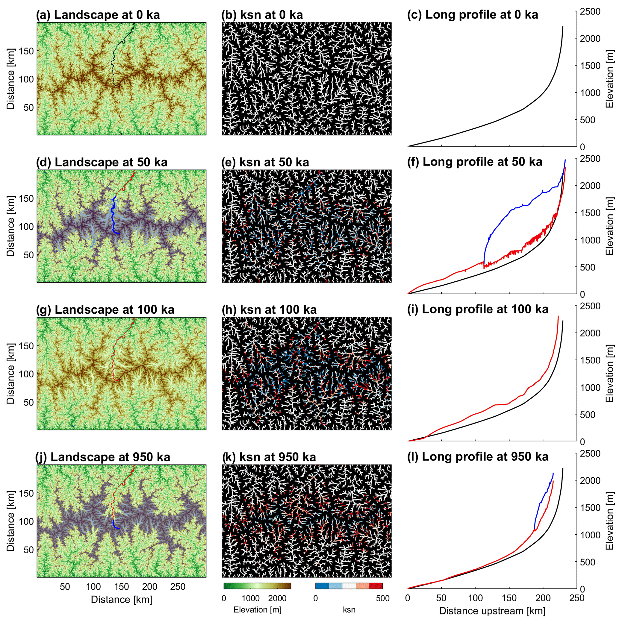
Figure 14Glacial landscape transformation of a mountain range over 10 total 100 ka cycles. Plotted stages refer to the initial fluvial topography, the first glacial maximum (50 ka), the first interglacial (100 ka) and 10th glacial maximum (950 ka). The ice cover is highlighted in light blue in the maps. The long profiles refer to the longest river, which is also drawn in the maps. Red lines describe the actual river profile, blue lines the ice surface and black lines the initial fluvial topography.
The model domain consists of 3000×2000 cells with a cell size of 100 m (Fig. 14). While the southern and northern boundaries are kept at zero elevation, periodic boundary conditions are used at the western and eastern boundaries. A uniform uplift rate U=0.625 mm a−1 was assumed and the respective fluvial steady-state topography was used as an initial state. In contrast to the previous experiments, uplift is maintained over the entire simulation covering 10 cycles of glaciation. Mass balance parameters are chosen to result in a sinusoidal variation of the ELA between 1950 and 2950 m with a period of 100 kyr. All other climatic parameters were adopted from the calibration performed in Sect. 3.2.
The fluvial steady-state topography features a contiguous, largely west–east-trending central ridge line (representing the principal drainage divide) with a maximum elevation of 3365 m (Fig. 14a).
The longitudinal extent of the glaciers in the individual valleys shows strong variations, in particular during the first period of glaciation (t=50 ka, Fig. 14d). It is related to the high sensitivity to the glacial mass balance already observed in Sect. 3.2. There it was found that even small changes in the model describing the melt rate strongly affect the glacial extent, meaning that it had to be adjusted carefully in order to keep the two models consistent. Similarly, the size and shape of the individual catchment have a strong influence on the mass balance. In this example, the longest glacier indeed occurs in the largest catchment, but some other large catchments experience little glaciation. So there seem to be properties beyond the catchment size that are responsible for the susceptibility to strong glaciation. In particular, the supply of ice by tributaries with high-elevation catchments may help the glaciers to persist over long distances. However, recognizing which catchments are particularly prone to massive glaciation from the fluvial topography alone (Fig. 14a) is not trivial and would go beyond the scope of this study.
Changes in river-long profiles can be quantified conveniently by the so-called normalized steepness index
For the initial fluvial equilibrium topography used here, it has a constant value of ksn=250 m in the entire domain. Since ksn is directly proportional to the channel slope S, maps of ksn reveal where and how much the valley-long profiles have become steeper or less steep compared to the fluvial equilibrium topography. The middle column of Fig. 14 shows maps of ksn where only sites with a catchment size A≥10 km2 are considered for clarity.
In particular during the first glaciation cycle, a rapid transformation from fluvial to glacial valley geometries occurs, which is indicated by distinct deviations in ksn from fluvial steady-state conditions (Fig. 14e). Ice-covered trunk valleys predominantly show a decrease in channel steepness, while the ice-free continuations of these valleys become steeper. There is no clear trend towards steeper or less steep channels in the middle reaches but a distinct decrease in channel steepness in the headwater regions. Surprisingly, the main changes in channel steepness are not owing to the incision of major valleys but to the deposition of glacier-borne sediments that come mainly from the valley flanks. The sediment flux at the glacier terminus exceeds the transport capacity of the contiguous river by far and causes extensive deposition of glacial sediments at the transition from the glacier to the river. Advancing glaciers overrun this thick layer of sediment and erode it again, but bedrock incision occurs only at the headwaters. This characteristic sequence of deposition and erosion, well known in natural glacio-fluvial systems, can be observed strikingly along the largest valley (Fig. 14f). Over more than 200 km of the lower reaches, and thus more than 90 % of the main valley, is still covered by more than 100 m thick sediments at the first glacial maximum. This results in a valley floor being significantly higher than those at the fluvial steady state. Note that uplift amounts only about 30 m from the simulation start to the first glacial maximum. The steep segment close to the outlet marks the transition from the sediment-filled valley to the stable base level of the model boundary.
With climate warming, the glaciers have largely retreated at t = 100 ka and fluvial incision dominates the evolution of mountain topography (Fig. 14g–i). However, fluvial erosion shows strong spatial variations. The steep river segments that originally formed near the model boundary feature erosion rates distinctly exceeding uplift rates. As the rivers erode the sediments, the steep segments migrate upstream and leave behind steady-state channel segments. Further upstream, the valleys are characterized by flat valley floors indicating hundreds of meters of valley infill. Due to the low channel length gradients in these sections, fluvial erosion is almost zero, which eventually leads to an increase in the elevation of the upper reaches.
Further glacial cycles successively reduce the area at high elevations, leading to a substantial decrease in ice production and ultimately to smaller glacial advances at the peak of the cold period (Fig. 14j–l; see also supplementary video – video03; https://doi.org/10.5281/zenodo.6557805). After 10 glacial cycles (t=950 ka), large parts of the mountain range are controlled by fluvial erosion even during cold climate conditions. As the extent of glacial occupation is much smaller than during the first glacial cycle and glacial valley widening is largely completed with the first glaciation, sediment delivery from the glaciers to the rivers is distinctly reduced, which leads to the situation that large parts of the drainage system are at or close to fluvial steady state. Channels at mid-altitudes with glaciers in their headwaters are still distinctly affected by the delivery of sediments and hence systematically steeper, as both uplift and sediment delivery rate have to be balanced by the fluvial erosion rate. In contrast, headwaters that are directly affected by glacial erosion show a reduced channel steepness (Fig. 14k).
However, these results should be interpreted cautiously. In our experiment, we assume that the sediments have the same erodibility as the bedrock, which is most likely inaccurate and overestimates the duration of excavating the valley fill strongly. Furthermore, erosion by the glaciers is based entirely on detachment-limited conditions. However, it can be assumed that transport-limited conditions prevail at least in some parts of the glacier where a till layer would protect the bed from further erosion, resulting in lower sediment production overall. In this sense, further studies with different parameter sets are needed to provide sufficient insight into the modeling of the complex system of joint fluvial and glacial mountain denudation, which is beyond the scope of this benchmark study.
The implementation of glacial erosion in OpenLEM relies on several simplifications. While some of these simplifications are approximations, some are rather ad hoc assumptions. The glacial stream power model can be seen as the core of the model. This stream power law was derived by simplifying existing relations for ice dynamics (flow and erosion) in combination with a parameterization of glacier width. As stated by Hergarten (2021a), the parameterization of glacier width is not fully based on existing empirical relations but relies on intuition to some extent. However, our numerical results on glacier-long profiles and glacier width are well in line with the results obtained from iSOSIA. Thus, the glacial stream power law in itself seems not to introduce a major limitation for typical alpine glaciers, at least not for the linear model (n=1). Neglecting the deformation of ice in OpenLEM seems to be the most critical point here. It leads to a moderate overestimation of glacial erosion at large ice fluxes. This issue was already discussed by Hergarten (2021a), and a possible solution was proposed in that study. Alternatively, the version of the glacial stream power law proposed by Deal and Prasicek (2021) avoids this problem. However, an extension in this direction is not yet available in OpenLEM and could thus not be tested. On the other hand, the overestimation of erosion rates at large ice fluxes is not crucial compared to the points discussed in the following.
As a main result of our comparison, it turned out that the components around the glacial stream power law are more critical than the glacial stream power law itself. While these components are necessary for setting up a 2-D landform evolution model, they rely on ad hoc assumptions to a large extent.
The model for the glacial mass balance (and thus for production and melting of ice) may be mentioned first in this context. The default approach for melting implemented in OpenLEM turned out not to reproduce the pattern of glaciation predicted by iSOSIA. However, OpenLEM is not an all-in-one model that attempts to capture all influences on glacial erosion. In the spirit of OpenLEM, the glacial mass balance is instead an external component. Therefore, OpenLEM offers users the opportunity to define their own models for the rate of melting. Our tests have shown that the model for the mass balance implemented in iSOSIA can be transferred to OpenLEM reasonably well. In any case, however, the glacial occupation and the resulting erosion are very sensitive to the mass balance, which also applies to iSOSIA (Pedersen and Egholm, 2013). Hence, a model-based reconstruction of the glacial history of real orogens is challenging and involves considerable uncertainties even without taking into account topographic changes (Seguinot et al., 2018). In the realm of simulations starting from synthetic topographies, however, these uncertainties are not crucial as long as the fundamental interactions between glacial erosion and topography are captured fairly well. In this context, the main difference between the two models is that iSOSIA derives the mass balance directly from more or less well-constrained climatic parameters, while users of OpenLEM are rather left alone in defining the model for the mass balance. However, the calibration obtained in Sect. 3.2.1 may be helpful for future studies.
The most serious limitations of OpenLEM arise from the simplified treatment of the ice surface. While physically based numerical models of ice flow consider the free ice surface as a variable, OpenLEM adopts a numerical scheme originally designed for fluvial erosion, where the deviation of the free water surface from the topography is neglected. The numerical scheme was extended in OpenLEM in such a way that the ice surface is not necessarily parallel to the topography. However, as the ice thickness is parameterized by the ice flux, gradients of the bedrock topography and the overlying ice surface are similar. Thus, the glaciers in OpenLEM are somewhere between glaciers with a free surface (as in iSOSIA) and artificially widened rivers in terms of their properties. However, we must keep in mind that the applications for which OpenLEM was developed do not explicitly require the simulation of ice patterns on a surface but aim to predict the evolution of landforms on large scales.
As a main consequence of the simple parameterization, the thickness of the ice is constant across the valley, regardless of its shape. As discussed in Sect. 3.2.3, this results in valleys with a quite flat floor and almost vertical walls, while glacial valleys simulated by iSOSIA are rather parabolic. However, iSOSIA is also not free of problems concerning the cross-sectional shape of valleys. Since its numerical performance breaks down if landforms become steep, the slopes practically have to be limited by adding hillslope processes to the model. Overall, the cross-sectional shape of valleys may be more realistic in iSOSIA than in OpenLEM, but we should be careful when defining a reference shape. In addition, we should keep in mind that the erosion model used in iSOSIA is finally rather simple, which may also affect the shape of the valleys (e.g., Ugelvig et al., 2016; Egholm et al., 2017; Bernard et al., 2021).
Beyond the cross-sectional shape of the valleys, the timescale of the conversion of a V-shaped fluvial valley into a U-shaped glacial valley is an issue in OpenLEM. The constant ice thickness results in a steep inclination of the ice surface towards the cardinal flow line and thus in high erosion rates during the early phase of glaciation. These erosion rates are considerably higher than in iSOSIA and lead to a faster transformation to a U-shaped valley. Although erosion rates are indeed assumed to be high when topography is not yet adapted to glacial conditions (e.g., Harbor, 1992), it is difficult to evaluate the model-specific differences because it is still unclear where individual processes and net erosion are most effective in natural landscapes (e.g., Alley et al., 2019). However, the speed of the adjustment is owing to adopting the glacial stream power law for the across-valley slope, which lacks a clear physical basis. Thus, the transformation into a U-shaped valley may be too fast in OpenLEM. Noteworthy, this is not a matter of calibrating parameter values since the timescale of adjustment is inherently linked to the erosion along the cardinal flow line.
The fast transformation into U-shaped valleys also affects the glacial mass balance since the average elevation of the ice surface across the valley decreases rapidly. As the glacial mass balance is very sensitive to this elevation, a strong retreat of the glaciers is observed during the initial phase. This retreat is not unrealistic in itself and also occurs in iSOSIA, although it is weaker there. In combination with the rapid change in cross-sectional shape, however, it results in a considerable part of the valley being shaped by a short but intense glaciation. This effect is in contrast to the prediction of iSOSIA and probably unrealistic.
In sum, assuming a constant ice thickness across the valleys appears to be the most important source of limitations in OpenLEM. This simplification also affects the pattern of erosion along the valleys. Here the parameterization of the thickness by the ice flux does not enforce a constant thickness, but still restricts the dynamic evolution of the ice surface. While this simple approach is able to predict overdeepened valleys at locations where the ice flux rapidly decreases downstream, it cannot reproduce the smoothing effect of the ice surface. As a consequence, steep gradients in the ice surface may also occur along the valley, which are transferred rapidly to the topography of the bedrock. Since the glacial stream power law inherited concepts from fluvial erosion, distinct knickpoints are formed and move upstream. This behavior is typical for rivers but not observed in simulations with iSOSIA. So some of the properties of glaciers in OpenLEM are closer to what we expect for rivers than to what we expect for glaciers. However, the example with the artificial boundary condition investigated in Sect. 3.1.3 is extreme, and we did not observe such strong effects in the subsequent scenarios. Nevertheless, effects of steep gradients in the ice surface should be kept in mind as a potential source of artifacts and bear some potential for future improvement. Deal and Prasicek (2021) proposed an approach to compute the ice surface at a moderate numerical effort if the ice flux is given. Since this approach avoids steep gradients, it would be worth finding out whether it harmonizes with the concept of the cardinal flow line implemented in OpenLEM.
In the context of sudden changes, the steady-state approximation for the ice flux should also be questioned. It implies that a rapid cooling immediately results in a fully developed pattern of glaciers. This concept was also inherited from the fluvial model. While effects of climatic changes on water fluxes indeed propagate almost instantaneously through rivers, the reference simulations with iSOSIA show that the response times of glaciers to sudden climatic changes are instead hundreds to thousands of years. Hence, high-frequency fluctuations in climate are strongly damped by the inertia of the natural system (Herman et al., 2018), but this damping is not captured by OpenLEM. While it is not clear to what extent this is a problem for long-term landform evolution, replacing the steady-state approximation in OpenLEM with a finite response time might also help to reduce the overestimation of the initial retreat of the glaciers. Thus, introducing a finite response time may be another option for future improvement.
The fundamental question concerning future developments of OpenLEM is whether extending it or improving the existing components is more promising. At the present level, the implementation of glacial erosion in OpenLEM is some kind of minimum model, while iSOSIA offers several extensions. Glacial hydrology is probably the most important extension since the fluid pressure at the bed has a strong influence on the sliding velocity and thus on glacial erosion (Herman et al., 2011; Egholm et al., 2012). On the other hand, reasonable results were also obtained from glacial erosion models without taking into account hydrology explicitly (Harbor, 1992; Egholm et al., 2011; Braun et al., 1999; Braedstrup et al., 2016). Taking into account the deformation of ice would be another useful extension. In turn, the results of our benchmarking experiments suggest that working on the issues arising from the constant ice thickness across the valley is more urgent. It is, however, not yet clear whether this is possible without losing the simplicity and the high numerical performance of the current implementation.
Given that the limitations arising from the simple parameterization of the ice thickness cannot be overcome soon, we should be clear what the fields of application of both models are in their present state. While the numerical implementation of the glacial stream power law is not a comprehensive model for the evolution of glacial landforms, it allows for a whole new group of experiments. It is therefore intended more as a complement to dynamic ice models such as iSOSIA. The latter allows the incorporation of sophisticated models for, e.g., glacial hydrology, basal sliding, sediment transport, thermal heat flow and glacial erosion. However, describing the individual processes in detail requires a large number of parameters. Empirical evidence to constrain these parameters is often lacking, which in turn limits our ability to determine the controlling factors of how glaciers erode topography. In contrast, the glacial stream power law as implemented in OpenLEM requires only a few parameters, which facilitates the interpretation of possible feedbacks and greatly improves the computational performance, meaning that temporal and spatial scales are no longer limiting factors in modeling glacial landform evolution.
The principal application field of OpenLEM is studying the relationship between glacier erosion, climate and topography at large spatial and temporal scales by roughly approximating the structure of alpine glacier networks (Sect. 3.5). Small-scale studies of form–process interactions that eventually improve our understanding of the evolution of individual glacial landforms (e.g., Egholm et al., 2017; Bernard et al., 2021) are limited to models such as iSOSIA because they are able to adjust ice flow and accurately resolve variations in basal shear stress as valley geometries change (Braedstrup et al., 2016). However, benchmarking experiments (Sect. 3.2) have shown that, apart from local differences in erosion, the conversion of fluvial to glacial landscapes produces a consistent glacial signal in topography in both models, which is also in agreement with natural examples (e.g., Liebl et al., 2021; Robl et al., 2015, 2017).
The seamless coupling of fluvial and glacial processes enables the investigation of the regional effects of glaciation on sediment transport and deposition, flexural isostasy, and orographic precipitation over millions of years. In this way, a simple model of glacial erosion, which has strong similarities to a model for fluvial erosion, provides an opportunity to interpret the evolutionary state of glacial imprinted mountain topography. Filling this research gap in the field of tectonic geomorphology is urgently needed because so far there are only a few approaches that provide theory (Headley et al., 2012; Prasicek et al., 2020b; Deal and Prasicek, 2021) and application (Pedersen et al., 2010; Liebl et al., 2021; Robl et al., 2015).
The stream power law for glacial erosion and its implementation into the 2-D landform evolution model OpenLEM (Hergarten, 2021a) were recently developed with special relevance for understanding the large-scale topographic signature of glacial erosion in alpine regions. Even though the ice flow dynamics are not directly computed, OpenLEM performs well in describing the fluvial to glacial landscape transformation. Benchmark experiments against the higher‐order ice sheet model iSOSIA (Egholm et al., 2011) show that both models produce a consistent glacial topographic signal with U-shaped valley cross sections and a valley length geometry with flat valley floors and distinct knickpoints at confluences. Erosion rates and the altitudinal adjustment of channel slopes and relief with glacial occupation time are largely consistent in both models. The major uncertainties are due to the ad hoc treatment of the valley shape in OpenLEM. The parameterization of the glacier width inhibits the investigation of feedbacks between form and processes at small scales. However, the consistency of characteristic glacial-valley-long profiles in both models provide a solid basis to investigate the topographic signal of glacial erosion at the scale of a mountain range. So far, large temporal and spatial scales in concert with a high spatial resolution have been limiting factors in modeling glacial landform evolution. The glacial stream power law implemented in OpenLEM has a computational effort that is only moderately larger than its fluvial counterpart. Hence, it is orders of magnitude more efficient than the also very efficient iSOSIA models. The superior computational performance allows for mountain-range-scale simulations in a coupled glacio-fluvial system over several glacial–interglacial cycles on standard desktop computers. The first promising results of this study indicate new research avenues by exploring the influence of tectonics and climate on mountain topography and the supporting crust over million-year timescales.
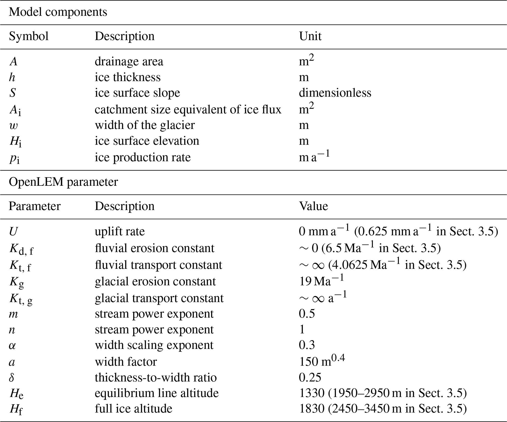
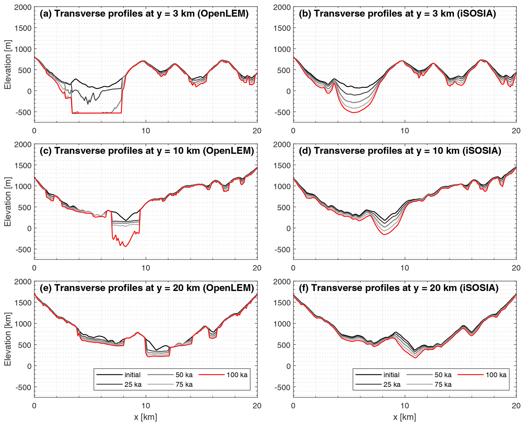
Figure B1Time series of the evolution of the transverse profiles in the OpenLEM and iSOSIA experiment (Sect. 3.1) at 3, 10 and 20 km upstream of the longitudinal swath profile.

Figure B2Differences in the evolving topography based on the width factor of the initial ice configuration of experiment (Sect. 3.2). (a–c) Evolving topographies with varying width factors (a=125, 150 and 175 m0.4) after 100 ka. (d–f) Ice configuration after 4 ka for each width factor. The same width to depth ratio of 0.25 is used in all three experiments. Spacing of contour lines in (a–c) is 200 m.
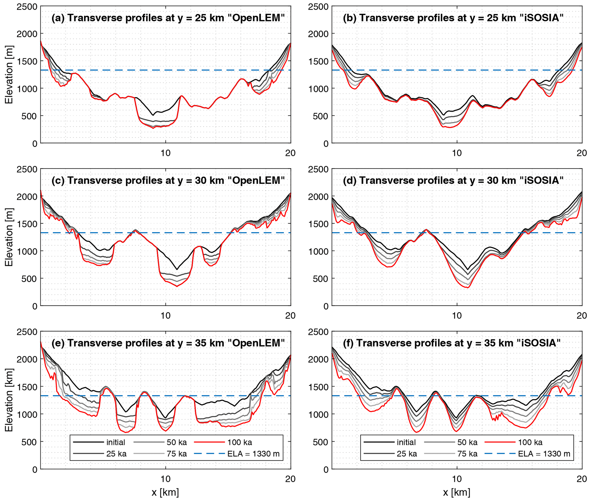
The code used for and results of the simulations are available at https://doi.org/10.5281/zenodo.6557805 (Liebl, 2022). The latest version of the open-source landform evolution model OpenLEM is freely available at http://hergarten.at/openlem (Hergarten, 2023). The authors are happy to assist interested readers in reproducing the results and performing subsequent research.
The video supplement includes the time-dependent simulations of the developing overdeepenings of experiment 1.1 (video01), and the respective landscape evolution of experiments 1.2 (video02-OpenLEM and video02-iSOSIA) and 3 (video03). It is available online at https://doi.org/10.5281/zenodo.6557805 (Liebl, 2022).
ML, JR and SH designed the study. The models iSOSIA and OpenLEM with the supervision to use them were provided by DLE and SH, respectively. ML conducted the experiments. ML, JR and SH prepared the manuscript with contributions from co-authors. Acquisition of funding was done by JR and KS. All authors have read and agreed to the final version of the manuscript.
The contact author has declared that none of the authors has any competing interests.
Publisher's note: Copernicus Publications remains neutral with regard to jurisdictional claims in published maps and institutional affiliations.
The authors would like to thank Leif S. Anderson and Eric Deal for their constructive comments and Andrew Wickert for the editorial handling.
This research has been supported by the Austrian Science Fund (grant no. P 31609) and the Salzburger Landesregierung (grant no. P 31609).
This paper was edited by Andrew Wickert and reviewed by Eric Deal and Leif S. Anderson.
Alley, R. B., Cuffey, K. M., and Zoet, L. K.: Glacial erosion: status and outlook, Ann. Glaciol., 60, 1–13, https://doi.org/10.1017/aog.2019.38, 2019. a, b
Anderson, R. S., Molnar, P., and Kessler, M. A.: Features of glacial valley profiles simply explained, J. Geophys. Res.-Earth, 111, F01004, https://doi.org/10.1029/2005jf000344, 2006. a
Bahr, D. B.: Width and length scaling of glaciers, J. Glaciol., 43, 557–562, https://doi.org/10.3189/S0022143000035164, 1997. a
Bernard, M., Steer, P., Gallagher, K., and Egholm, D. L.: The Impact of Lithology on Fjord Morphology, Geophys. Res. Lett., 48, e2021GL093101, https://doi.org/10.1029/2021GL093101, 2021. a, b, c
Brædstrup, C. F., Egholm, D. L., Ugelvig, S. V., and Pedersen, V. K.: Basal shear stress under alpine glaciers: insights from experiments using the iSOSIA and Elmer/Ice models, Earth Surf. Dynam., 4, 159–174, https://doi.org/10.5194/esurf-4-159-2016, 2016. a, b, c, d, e, f, g
Braun, J., Zwartz, D., and Tomkin, J. H.: A new surface-processes model combining glacial and fluvial erosion, Ann. Glaciol., 28, 282–290, https://doi.org/10.3189/172756499781821797, 1999. a, b, c, d
Brocklehurst, S. H. and Whipple, K. X.: Hypsometry of glaciated landscapes, Earth Surf. Proc. Land., 29, 907–926, https://doi.org/10.1002/esp.1083, 2004. a
Budd, W. F., Keage, P. L., and Blundy, N. A.: Empirical Studies of Ice Sliding, J. Glaciol., 23, 157–170, https://doi.org/10.3189/S0022143000029804, 1979. a
Cook, S. J., Swift, D. A., Kirkbride, M. P., Knight, P. G., and Waller, R. I.: The empirical basis for modelling glacial erosion rates, Nat. Commun., 11, 1–7, https://doi.org/10.1038/s41467-020-14583-8, 2020. a
Cuffey, K. M. and Paterson, W. S. B.: The physics of glaciers, Academic Press, ISBN 9780123694614, 2010. a, b, c
Davy, P. and Lague, D.: Fluvial erosion/transport equation of landscape evolution models revisited, J. Geophys. Res.-Earth, 114, F03007, https://doi.org/10.1029/2008JF001146, 2009. a
Deal, E. and Prasicek, G.: The sliding ice incision model: A new approach to understanding glacial landscape evolution., Geophys. Res. Lett., 48, e2020GL089263, https://doi.org/10.1029/2020GL089263, 2021. a, b, c, d, e, f, g, h, i, j
Egholm, D. L., Nielsen, S. B., Pedersen, V. K., and Lesemann, J. E.: Glacial effects limiting mountain height, Nature, 460, 884–887, https://doi.org/10.1038/nature08263, 2009. a
Egholm, D. L., Knudsen, M. F., Clark, C. D., and Lesemann, J. E.: Modeling the flow of glaciers in steep terrains: The integrated second‐order shallow ice approximation (iSOSIA), J. Geophys. Res.-Earth, 116, F02012, https://doi.org/10.1029/2010JF001900, 2011. a, b, c, d, e, f, g, h
Egholm, D. L., Pedersen, V. K., Knudsen, M. F., and Larsen, N. K.: Coupling the flow of ice, water, and sediment in a glacial landscape evolution model, Geomorphology, 141–142, 47–66, https://doi.org/10.1016/j.geomorph.2011.12.019, 2012. a, b, c, d, e, f
Egholm, D. L., Jansen, J. D., Braedstrup, C. F., Pedersen, V. K., Andersen, J. L., Ugelvig, S. V., Larsen, N. K., and Knudsen, M. F.: Formation of plateau landscapes on glaciated continental margins, Nat. Geosci., 10, 592–597, https://doi.org/10.1038/Ngeo2980, 2017. a, b, c, d
Fowler, A. C. and Larson, D. A.: On the flow of polythermal glaciers – I. Model and preliminary analysis, Proc. R. Soc. Lond., 363, 217–242, https://doi.org/10.1098/rspa.1978.0165, 1978. a
Hallet, B.: A theoretical model of glacial abrasion, J. Glaciol., 23, 39–50, https://doi.org/10.3189/S0022143000029725, 1979. a
Harbor, J. M.: Numerical modeling of the development of U-shaped valleys by glacial erosion, Geol. Soc. Am. Bull., 104, 1364–1375, https://doi.org/10.1130/0016-7606(1992)104<1364:Nmotdo>2.3.Co;2, 1992. a, b, c
Headley, R. M., Roe, G., and Hallet, B.: Glacier longitudinal profiles in regions of active uplift, Earth Planet. Sci. Lett., 317, 354–362, 2012. a
Hergarten, S.: Transport-limited fluvial erosion – simple formulation and efficient numerical treatment, Earth Surf. Dynam., 8, 841–854, https://doi.org/10.5194/esurf-8-841-2020, 2020. a, b
Hergarten, S.: Modeling glacial and fluvial landform evolution at large scales using a stream-power approach, Earth Surf. Dynam., 9, 937–952, https://doi.org/10.5194/esurf-9-937-2021, 2021a. a, b, c, d, e, f, g, h, i, j, k, l, m, n, o, p, q
Hergarten, S.: The influence of sediment transport on stationary and mobile knickpoints in river profiles, J. Geophys. Res.-Earth, 126, e2021JF006218, https://doi.org/10.1029/2021JF006218, 2021b. a, b, c
Hergarten, S.: Theoretical and numerical considerations of rivers in a tectonically inactive foreland, Earth Surf. Dynam., 10, 671–686, https://doi.org/10.5194/esurf-10-671-2022, 2022. a
Hergarten, S.: OpenLEM, OpenLEM [code], http://hergarten.at/openlem, last access: 20 February 2023. a
Hergarten, S. and Robl, J.: The linear feedback precipitation model (LFPM 1.0) – a simple and efficient model for orographic precipitation in the context of landform evolution modeling, Geosci. Model Dev., 15, 2063–2084, https://doi.org/10.5194/gmd-15-2063-2022, 2022. a, b
Hergarten, S., Wagner, T., and Stüwe, K.: Age and prematurity of the Alps derived from topography, Earth Planet. Sci. Lett., 297, 453–460, https://doi.org/10.1016/j.epsl.2010.06.048, 2010. a
Herman, F., Beaud, F., Champagnac, J.-D., Lemieux, J.-M., and Sternai, P.: Glacial hydrology and erosion patterns: A mechanism for carving glacial valleys, Earth Planet. Sci. Lett., 310, 498–508, 2011. a, b
Herman, F., Beyssac, O., Brughelli, M., Lane, S. N., Leprince, S., Adatte, T., Lin, J. Y. Y., Avouac, J. P., and Cox, S. C.: Erosion by an Alpine glacier, Science, 350, 193–195, https://doi.org/10.1126/science.aab2386, 2015. a, b
Herman, F., Braun, J., Deal, E., and Prasicek, G.: The Response Time of Glacial Erosion, J. Geophys. Res.-Earth, 123, 801–817, https://doi.org/10.1002/2017JF004586, 2018. a
Howard, A. D.: A detachment-limited model for drainage basin evolution, Water Resour. Res., 30, 2261–2285, https://doi.org/10.1029/94WR00757, 1994. a, b
Hutter, K.: Time-dependent surface elevation of an ice slope, J. Glaciology, 25, 247–266, https://doi.org/10.3189/S0022143000010479, 1980. a
Iverson, N. R.: A theory of glacial quarrying for landscape evolution models, Geology, 40, 679–682, https://doi.org/10.1130/G33079.1, 2012. a
Kooi, H. and Beaumont, C.: Large-scale geomorphology: classical concepts reconciled and integrated with contemporary ideas via a surface process model, J. Geophys. Res., 101, 3361–3386, 1996. a
Koppes, M., Hallet, B., Rignot, E., Mouginot, J., Wellner, J. S., and Boldt, K.: Observed latitudinal variations in erosion as a function of glacier dynamics, Nature, 526, 100–103, https://doi.org/10.1038/nature15385, 2015. a, b
Kühni, A. and Pfiffner, O. A.: The relief of the Swiss Alps and adjacent areas and its relation to lithology and structure: topographic analysis from a 250-m DEM, Geomorphology, 41, 285–307, https://doi.org/10.1016/S0169-555x(01)00060-5, 2001. a
Lai, J. and Anders, A. M.: Climatic controls on mountain glacier basal thermal regimes dictate spatial patterns of glacial erosion, Earth Surf. Dynam., 9, 845–859, https://doi.org/10.5194/esurf-9-845-2021, 2021. a, b
Leith, K., Moore, J. R., Amann, F., and Loew, S.: Subglacial extensional fracture development and implications for Alpine valley evolution, J. Geophys. Res.-Earth, 119, 62–81, https://doi.org/10.1002/2012JF002691, 2014. a
Liebl, M.: C++ (OpenLEM, v37), C (iSOSIA, v3.4.3) and Matlab codes, Zenodo [code and data set], https://doi.org/10.5281/zenodo.6557805, 2022. a, b
Liebl, M., Robl, J., Egholm, D. L., Prasicek, G., Stüwe, K., Gradwohl, G., and Hergarten, S.: Topographic signatures of progressive glacial landscape transformation, Earth Surf. Proc. Land., 46, 1964–1980, https://doi.org/10.1002/esp.5139, 2021. a, b, c, d, e, f
Magrani, F., Valla, P. G., and Egholm, D.: Modelling alpine glacier geometry and subglacial erosion patterns in response to contrasting climatic forcing, Earth Surf. Proc. Land., 47, 1054–1072, https://doi.org/10.1002/esp.5302, 2022. a, b, c
O'Callaghan, J. F. and Mark, D. M.: The extraction of drainage networks from digital elevation data, Comput. Vision Graph., 28, 323–344, https://doi.org/10.1016/S0734-189X(84)80011-0, 1984. a
Pedersen, V. K. and Egholm, D. L.: Glaciations in response to climate variations preconditioned by evolving topography, Nature, 493, 206–210, https://doi.org/10.1038/nature11786, 2013. a, b, c
Pedersen, V. K., Egholm, D. L., and Nielsen, S. B.: Alpine glacial topography and the rate of rock column uplift: a global perspective, Geomorphology, 122, 129–139, https://doi.org/10.1016/j.geomorph.2010.06.005, 2010. a, b
Penck, A.: Glacial features in the surface of the Alps, J. Geol., 13, 1–19, 1905. a
Prasicek, G., Larsen, I. J., and Montgomery, D. R.: Tectonic control on the persistence of glacially sculpted topography, Nat. Commun., 6, 8028, https://doi.org/10.1038/ncomms9028, 2015. a
Prasicek, G., Hergarten, S., Deal, E., Herman, F., and Robl, J.: A glacial buzzsaw effect generated by efficient erosion of temperate glaciers in a steady state model, Earth Planet. Sci. Lett., 543, 116350, https://doi.org/10.1016/j.epsl.2020.116350, 2020a. a
Prasicek, G., Hergarten, S., Deal, E., Herman, F., and Robl, J.: A glacial buzzsaw effect generated by efficient erosion of temperate glaciers in a steady state model, Earth Planet. Sci. Lett., 543, 116350, https://doi.org/10.1016/j.epsl.2020.116350, 2020b. a, b
Robl, J., Prasicek, G., Hergarten, S., and Stüwe, K.: Alpine topography in the light of tectonic uplift and glaciation, Glob. Planet. Change, 127, 34–49, https://doi.org/10.1016/j.gloplacha.2015.01.008, 2015. a, b, c, d
Robl, J., Hergarten, S., and Prasicek, G.: The topographic state of fluvially conditioned mountain ranges, Earth Sci. Rev., 168, 290–317, https://doi.org/10.1016/j.earscirev.2017.03.007, 2017. a
Robl, J., Hergarten, S., and Prasicek, G.: Glacial erosion promotes high mountains on thin crust, Earth Planet. Sci. Lett., 538, 116196, https://doi.org/10.1016/j.epsl.2020.116196, 2020. a
Roering, J. J., Kirchner, J. W., and Dietrich, W. E.: Evidence for nonlinear, diffusive sediment transport on hillslopes and implications for landscape morphology, Water Resour. Res., 35, 853–870, https://doi.org/10.1029/1998wr900090, 1999. a
Royden, L. and Perron, J. T.: Solutions of the stream power equation and application to the evolution of river longitudinal profiles, J. Geophys. Res.-Earth, 118, 497–518, https://doi.org/10.1002/jgrf.20031, 2013. a
Salcher, B., Prasicek, G., Baumann, S., and Kober, F.: Alpine relief limited by glacial occupation time, Geology, 49, 1209–1213, https://doi.org/10.1130/G48639.1, 2021. a
Salcher, B. C., Kober, F., Kissling, E., and Willett, S. D.: Glacial impact on short-wavelength topography and long-lasting effects on the denudation of a deglaciated mountain range, Global Planet. Change, 115, 59–70, https://doi.org/10.1016/j.gloplacha.2014.01.002, 2014. a
Schwanghart, W. and Kuhn, N. J.: TopoToolbox: A set of Matlab functions for topographic analysis, Environ. Modell. Softw., 25, 770–781, https://doi.org/10.1016/j.envsoft.2009.12.002, 2010. a
Schwanghart, W. and Scherler, D.: Short Communication: TopoToolbox 2 – MATLAB-based software for topographic analysis and modeling in Earth surface sciences, Earth Surf. Dynam., 2, 1–7, https://doi.org/10.5194/esurf-2-1-2014, 2014. a
Seguinot, J., Ivy-Ochs, S., Jouvet, G., Huss, M., Funk, M., and Preusser, F.: Modelling last glacial cycle ice dynamics in the Alps, The Cryosphere, 12, 3265–3285, https://doi.org/10.5194/tc-12-3265-2018, 2018. a, b
Sternai, P., Herman, F., Fox, M. R., and Castelltort, S.: Hypsometric analysis to identify spatially variable glacial erosion, J. Geophys. Res.-Earth, 116, F03001, https://doi.org/10.1029/2010jf001823, 2011. a
Sternai, P., Herman, F., Valla, P. G., and Champagnac, J.-D.: Spatial and temporal variations of glacial erosion in the Rhône valley (Swiss Alps): Insights from numerical modeling, Earth Planet. Sci. Lett., 368, 119–131, https://doi.org/10.1016/j.epsl.2013.02.039, 2013. a
Ugelvig, S., Egholm, D., and Iverson, N. R.: Glacial landscape evolution by subglacial quarrying: A multiscale computational approach, J. Geophys. Res.-Earth, 121, 2042–2068, https://doi.org/10.1002/2016jf003960, 2016. a, b, c, d, e, f
Ugelvig, S., Egholm, D., Anderson, R., and Iverson, N. R.: Glacial erosion driven by variations in meltwater drainage, J. Geophys. Res.-Earth, 123, 2863–2877, https://doi.org/10.1029/2018JF004680, 2018. a, b, c, d, e
Weertman, J.: On the Sliding of Glaciers, J. Glaciol., 3, 33–38, https://doi.org/10.3189/S0022143000024709, 1957. a
Whipple, K. X.: Bedrock rivers and the geomorphology of active orogens, Annu. Rev. Earth Planet. Sci., 32, 151–185, https://doi.org/10.1146/annurev.earth.32.101802.120356, 2004. a
Whipple, K. X. and Tucker, G. E.: Dynamics of the stream-power river incision model: Implications for height limits of mountain ranges, landscape response timescales, and research needs, J. Geophys. Res.-Sol. Ea., 104, 17661–17674, https://doi.org/10.1029/1999JB900120, 1999. a
Whipple, K. X. and Tucker, G. E.: Implications of sediment-flux-dependent river incision models for landscape evolution, J. Geophys. Res., 107, 2039, https://doi.org/10.1029/2000JB000044, 2002. a
Wobus, C., Whipple, K. X., Kirby, E., Snyder, N., Johnson, J., Spyropolou, K., Crosby, B., and Sheehan, D.: Tectonics from topography: Procedures, promise, and pitfalls, in: Tectonics, Climate, and Landscape Evolution, edited by: Willett, S. D., Hovius, N., Brandon, M. T., and Fisher, D. M., vol. 398 of GSA Special Papers, 55–74, Geological Society of America, Boulder, Washington, D.C., https://doi.org/10.1130/2006.2398(04), 2006. a
- Abstract
- Introduction
- Considered models
- Benchmark scenarios
- Scope, limitations and perspectives
- Conclusions
- Appendix A: Model components
- Appendix B: Additional figures
- Code and data availability
- Video supplement
- Author contributions
- Competing interests
- Disclaimer
- Acknowledgements
- Financial support
- Review statement
- References