the Creative Commons Attribution 4.0 License.
the Creative Commons Attribution 4.0 License.
 | 23 Feb 2023
Barotropic tides in MPAS-Ocean (E3SM V2): impact of ice shelf cavities
Nairita Pal
Kristin N. Barton
Mark R. Petersen
Steven R. Brus
Darren Engwirda
Brian K. Arbic
Andrew F. Roberts
Joannes J. Westerink
Damrongsak Wirasaet
Oceanic tides are seldom represented in Earth system models (ESMs) owing to the need for high horizontal resolution to accurately represent the associated barotropic waves close to coasts. This paper presents results of tides implemented in the Model for Prediction Across Scales–Ocean or MPAS-Ocean, which is the ocean component within the U.S. Department of Energy developed Energy Exascale Earth System Model (E3SM). MPAS-Ocean circumvents the limitation of low resolution using unstructured global meshing. We are at this stage simulating the largest semidiurnal (M2, S2, N2) and diurnal (K1, O1) tidal constituents in a single-layer version of MPAS-O. First, we show that the tidal constituents calculated using MPAS-Ocean closely agree with the results of the global tidal prediction model TPXO8 when suitably tuned topographic wave drag and bottom drag coefficients are employed. Thereafter, we present the sensitivity of global tidal evolution due to the presence of Antarctic ice shelf cavities. The effect of ice shelves on the amplitude and phase of tidal constituents are presented. Lower values of complex errors (with respect to TPXO8 results) for the M2 tidal constituents are observed when the ice shelf is added in the simulations, with particularly strong improvement in the Southern Ocean. Our work points towards future research with varying Antarctic ice shelf geometries and sea ice coupling that might lead to better comparison and prediction of tides and thus better prediction of sea-level rise and also the future climate variability.
- Article
(7912 KB) - Full-text XML
- BibTeX
- EndNote


Ocean tides are generated due to the gravitational force from celestial bodies – the Sun, Moon and the Earth. Such gravitational dynamics causes the sea surface height of the global ocean to oscillate at well-defined amplitude and frequency (Mellor, 1996). These oscillations are dominated by diurnal (daily) and semidiurnal (twice daily) constituents or frequencies. The tide plays an important role in a broad range of global oceanic processes including oceanic mixing and heat, salt and biogeochemical (BGC) fluxes (Vic et al., 2019; Ledwell et al., 2000; Munk, 1997), sedimentation (Kidder, 2011), and biological processes and resulting habitats (Knox et al., 2018). Oceanic mixing due to tides, winds and waves contributes to the redistribution of heat from the Equator to the poles. Thus understanding and predicting tides and tidal mixing is essential to predicting global climate variability. Accurate representation of tides is necessary, not only to predict ocean currents and future climate variability but also to remove tidal noise during satellite altimetry or satellite gravimetry (Coleman, 2001; Zaron and DeCarvalho, 2016) since tidal signals affect different kinds of observational data, ranging from space geodetic observations to the measurement of ocean currents.
In this paper, we focus on the mechanical interactions of the ocean tides with the Antarctic ice shelf cavities. Needless to say, accurately representing such tidal interactions with ice shelves is indispensable in the current scenario of a warming climate, melting ice shelves and constantly evolving ice shelf geometries (De Kleermaeker et al., 2017; Blakely et al., 2022; Wang et al., 2021; Richter et al., 2022; Verfaillie et al., 2022). Ice shelves are permanent floating sheets of ice that are connected or “grounded” to a landmass (see Fig. 1). Most of the world's ice shelves hug the coast of Antarctica. However, ice shelves can also form wherever ice flows from land into cold ocean waters, including some glaciers in the Northern Hemisphere. The point at which the ice shelf loses contact with the bed is called the “grounding line”. This grounding line can migrate with the tide, due to the elastic interactions between the tides and ice or the tidal flexure on the surface of an ice shelf (Brunt et al., 2010; Padman et al., 2018). The region over which the ice shelf loses contact with the bedrock and just floats in open ocean is called the “grounding zone”, and in this region the ice shelves directly interact with oceans and thus ocean tides. There are a number of detailed works on ocean–ice-shelf interactions (Jacobs et al., 1992; Straneo et al., 2013; Warburton et al., 2020; Turner et al., 2017). In this work, we present the impacts of the Antarctic ice shelf cavities on the dynamics of global tides, simulated using the Los Alamos National Laboratory (LANL)-led global ocean model known as the Model for Prediction Across Scales–Ocean or MPAS-Ocean (Ringler et al., 2013; Petersen et al., 2015). We have modified MPAS-Ocean to work in a barotropic or “single-layer” framework to increase computational efficiency.
The barotropic, or single-layer, global tide model within MPAS-Ocean is supplemented with specific schemes to dissipate tidal energy. The total energy of the tidal motion in the oceans across the world is about 3.5 TW (Egbert and Ray, 2003), which was originally believed to be dissipated only through bottom friction in shallow coastal shelf seas (Taylor, 1920). Thus, in the early barotropic tide models the tidal dissipation term was either linear or quadratic bottom drag in the coastal oceans, with the drag coefficients appropriately tuned to match observations (Schwiderski, 1980; Le Provost et al., 1994). However, works of Egbert and Ray (2000) showed that about a third of the barotropic tidal dissipation occurs in the deep ocean, thus debunking previous assumptions that all tidal energy is dissipated in shallow water. Works of Munk (1966) and Munk and Wunsch (1998) established that baroclinic tides contribute strongly to tidal energy dissipation. Tidal currents flowing over topography in a stratified ocean can give rise to tidal-period oscillations, known as internal or baroclinic tides. In fact, energy is transferred from the barotropic to the baroclinic tide in rough topography (Munk and Wunsch, 1998). The energy conversion from barotropic to the baroclinic tide in rough topography is represented through a linear wave drag term (Stigebrandt, 1999; Jayne and St. Laurent, 2001). Such wave drags are commonly known as “internal wave drag” in the literature (Egbert et al., 2004; Arbic et al., 2004) and have been shown to improve tidal elevations by reducing root-mean-square elevation error with observations (Egbert et al., 2004; Arbic et al., 2004; Green and Nycander, 2013; Lyard et al., 2006). The internal wave drag scheme can be implemented with or without a tunable parameter. In our work, which is an early effort at introducing a linear wave drag scheme in a tide model implemented in MPAS-Ocean, we use a scalar wave drag formulation with a tunable parameter. Our scheme, originally implemented by Jayne and St. Laurent (2001), is based on a linear scaling relationship and strongly depends on a tunable parameter. As we show later, our tuning parameter essentially sets the length scale associated with dissipation.
Some drag schemes (Egbert et al., 2004) are derived using linear transformations of the bottom topography (Bell, 1975) and do not have a tunable parameter. Such schemes have been shown to perform better when applied to barotropic models, with global dissipation rates close to TPXO7.2 (Green and Nycander, 2013). However, the drawback of schemes without a tunable parameter is that the dissipation rates and root-mean-square errors strongly depend on the global bathymetry and stratification databases and thus do not guarantee an optimal prediction of elevation and dissipation rates. For example, bathymetric databases might not resolve all abyssal features. The analytically computed Nycander scheme has been shown to increase regional and global dissipation rates due to the inclusion of abyssal hill roughness on ocean spreading ridges (Melet et al., 2013). On the other hand, high-resolution bathymetric databases increase the linear wave drag strength indicating a need for more tuning (Nycander, 2005; Zilberman et al., 2009). The reason for such an increase in wave drag has been attributed to a supercritical topography (Nikurashin and Ferrari, 2011; Scott et al., 2011), but a tunable parameter is still needed to correct the effect.
The particular scalar drag scheme that we utilize in this study is the Jayne and St. Laurent (2001) scheme. This drag acts on a barotropic global ocean model forced with five major tidal constituents: M2, S2, N2, K1 and O1. We show that our model performs very well with respect to root-mean-square tidal elevation comparisons against TPXO8 data (https://doi.org/10.5281/zenodo.7084790; Pal, 2023). We present a sensitivity study using meshes of varying resolution and show that the root-mean-square error values improve when we use high-resolution meshes. In the last section of the paper, we focus on the mechanical interactions of the ocean tides with the Antarctic ice shelf cavities and show that inclusion of ice shelf cavities improves the tidal elevation comparison results against TPXO8 data.
One other important factor that must be accounted for in global tide models is the self-attraction and loading (SAL). SAL accounts for a combination of effects: the deformation of the Earth's crust due to mass loading and the self-gravitation of the load-deformed Earth as well as of the ocean tide itself (Hendershott, 1972). Self-attraction and loading can change tidal amplitudes to first order (up to 20 % in some regions) and also significantly impact tidal phases and amphidromic points (Gordeev et al., 1977). A full calculation of SAL calls for the convolution of tidal elevation with a proper Green's function or a multiplication with load Love numbers in the spectral – i.e., spherical harmonic – domain (Ray, 1998). However, due to computational efficiency, we have used a scalar SAL term in the major part of this study (Accad and Pekeris, 1978). A full calculation of SAL has been recently investigated in detail in Barton et al. (2023) and Brus et al. (2023).
The paper is organized as follows. In Sect. 2, we present a brief overview of our model components, with a focus on new modifications and developments within the MPAS-Ocean framework. In Sect. 3, we show some verification and validation results for our barotropic single-layer MPAS-Ocean ocean framework against analytical solutions from a planar two-dimensional ocean test case. We show that our barotropic ocean model reproduces known theoretical results. In Sect. 4, we present some background on TPXO8 data and the MPAS-Ocean mesh used for the simulations. In Sect. 5, we present the MPAS-Ocean model's sea surface elevation root-mean-square error results against observational TPXO8 data, the sensitivity of the results to different meshes, the impact of adding Antarctic ice shelf cavities, and the effect of adding a full (inline) self-attraction and loading term in our simulations. We finish our paper with discussions, conclusions and future directions in Sect. 6.
This work is a systematic analysis of tides implemented in MPAS-Ocean, including the addition of ice shelf cavities. MPAS-Ocean is the ocean component of the DOE's Energy Exascale Earth System Model (E3SM) (Golaz et al., 2019; Petersen et al., 2019) (we use E3SM version V2 here). MPAS-Ocean is solved using finite-volume methods (FVMs) on an unstructured grid, and this is where our work has an extra edge. The MPAS-Ocean code has the ability to run on unstructured meshes, which helps resolve sharp bathymetry critical for tides. This multi-resolution approach is built upon two key components: a variable-resolution mesh with exceptional mesh-quality characteristics and a finite-volume method that maintains all of its conservation properties even when implemented on a highly nonuniform grid. The unstructured variable-resolution mesh is required to resolve coastal processes in greater detail, while maintaining a relatively low resolution for the open-ocean processes which are relatively simpler to parameterize. Such variable resolution is achieved using the spherical centroidal Voronoi tessellations or SCVTs (Ringler et al., 2008). Numerical algorithms specifically designed for these grids guarantee that volume and energy are conserved (Ringler et al., 2010). The time-stepping scheme is the fourth-order Runge–Kutta method.
We present results of global tidal evolution over a number of horizontal mesh configurations, ranging from uniform 64 to 8 km configurations as well as variable-resolution designs. Such single-layer framework is ideal for a seamless implementation and testing of new features (e.g., the topographic wave drag and bottom friction schemes that we use). The governing momentum equations for MPAS-O that we use in our study are the shallow-water equations, written in so-called vector-invariant form (Ringler et al., 2010):
where u represents the depth-averaged horizontal velocity, t is the time coordinate, f is the Coriolis parameter, k is the vertical unit vector, is the kinetic energy, g is the gravitational acceleration constant, η is the sea surface height relative to the unperturbed ocean surface, ηEQ is the equilibrium tide, ηSAL is the perturbation of tidal elevations due to SAL, χ is a tunable scalar dimensionless wave drag coefficient, is a topographic wave drag timescale, H is the resting depth of the ocean, 𝒞D is the bottom friction coefficient, and h is the total ocean thickness such that . The full form of the drag terms in Eq. (1) would use the total thickness h, but our implementation uses the linearized version with the resting depth H. For the linear drag scheme, we use the formulation due to Jayne and St. Laurent (2001), with the inverse timescale computed according to Buijsman et al. (2016). Further details are provided in Sect. 2.3. Here ps represents the surface pressure on the ocean due to the floating ice shelf cavities (see Sect. 2.5), and p refers to the total pressure on the vertical column of water.
We have the following important modification to MPAS-Ocean in our model: (a) we introduce an external forcing due to astronomical tides (Barton et al., 2023; Brus et al., 2023); (b) we introduce a new drag scheme due to friction with the seabed representing the log law of wall turbulence and a new drag scheme called topographic wave drag due to scattering with rough topography; (c) dynamics due to Antarctic ice shelf cavities, together with a full inline SAL.
2.1 Tidal forcing
The tidal forcing is obtained from an astronomical potential among celestial bodies (see Barton et al., 2023, for details). Here we just state the governing equations for the sea surface height perturbation due to tides. The perturbation to the sea surface height ηEQ is a combination of principal semidiurnal and diurnal tides:
where these terms are valid for semidiurnal (sd) and diurnal (d) tidal constituents (Arbic et al., 2018). The total forcing comes from summing over each of the constituents, c. Here A and ω are the forcing amplitude and frequency, respectively, dependent on the tidal constituent; tref is a specified reference time; t is time; ϕ is latitude; λ is longitude; χ(tref) is an astronomical argument dependent on tidal constituent; and f(tref) and ν(tref) are amplitude and phase nodal factors accounting for small known astronomical modulations in the tidal forcing. represents the body tide Love numbers accounting for changes in the gravitational potential (k2) due to deformation of the Earth's crust and mantle from tidal forcing (h2).
2.2 Drag based on ocean bottom roughness
An ocean bottom-depth-based friction coefficient is important when we want to use a smaller value in deep water (for non-tidal energetic tuning, say) and a high value for tides in shallow regions. We implement a bottom friction coefficient based on the ocean bottom roughness, in the MPAS-Ocean model code. The friction coefficient CD in Eq. (1) is evaluated according to the following formula (Oey, 2006):
where κ=0.4 is the von Kármán constant (Von Kármán, 1931), z0 is the roughness parameter and zb is the ocean layer thickness (i.e., the sea surface height + the ocean bottom depth). CD,min is the minimum quadratic bottom friction coefficient. Typically, in previous studies, z0=10 mm and . The derivation of CD is given in Oey (2006) and is obtained by matching the near-bottom modeled velocity to the law of the wall (Schlichting and Gersten, 2016).
2.3 Topographic wave drag
As we discuss in the Introduction, we utilize the Jayne and St. Laurent (2001) scheme to calculate the topographic wave drag in this study. This is a scalar scheme, in which the wave drag strength is independent of the flow direction. Works by Egbert et al. (2004) show that the scalar scheme produces reasonable agreement with observations after being appropriately tuned. This scalar scheme is easier to implement than the more sophisticated tensor-based scheme (Nycander, 2005). In the tensor-based scheme, the tensor components are functions of the directionality of topographic roughness, and hence, the wave drag strength depends on the flow direction relative to the rough topography.
The term represents the topographic wave drag on the velocity u. The factor is an inverse timescale, and χ is a tunable drag coefficient. As we discussed in the Introduction, this is a scalar linear wave drag scheme, or the Jayne and St. Laurent formulation for wave drag (Jayne and St. Laurent, 2001; Buijsman et al., 2015):
Here is the bottom roughness, Nb is the buoyancy frequency at the bottom, and L is the wavelength of the bottom topography typically set as 10 km (Jayne and St. Laurent, 2001; Buijsman et al., 2015). We implement the wave drag term as χ𝒞u representing a linear drag on the velocity u. The factor 𝒞 () is a data field we obtain following the procedure described in Buijsman et al. (2015), and χ is a tunable drag coefficient. It is interesting to note here that after tuning, the optimum value of χ settles at a value between 1.08 and 1.44 for the high-resolution meshes, which is in the same range as the pre-factor in Eq. (7).
2.4 Self-attraction and loading (SAL)
In the first part of the work, SAL is implemented in MPAS-Ocean via the scalar approximation (Accad and Pekeris, 1978; Ray, 1998):
where η is the sea surface height prior to alterations and β=0.09 is a scalar parameter used to approximate the influence of SAL. This approximation is a computationally inexpensive method that is sufficiently accurate for many cases. However, this does not capture the spatial dependence and large-scale smoothing of the full calculation.
To capture the full spatial dependence, in the latter part of the paper, SAL is implemented as additional body force via the sea surface height gradient term in Eq. (1). As detailed in Barton et al. (2023), we express the inline SAL for tides in terms of the spherical harmonic decomposition of the sea surface height (Hendershott, 1972):
where each spherical harmonic sea surface height term ηn is multiplied by a scalar coefficient (Wang et al., 2012). Here ρ0 is the average density of seawater, ρearth is the average density of the solid Earth, and the multiplicative term represents load Love numbers corresponding to physical effects of SAL. The “1”, and terms account for gravitational self-attraction of the ocean, gravitational self-attraction of the deformed solid Earth, and deformation due to loading of the solid Earth, respectively. However, the usage of sea surface height for calculating SAL is only appropriate for tides and wind-driven barotropic motions. For other motions one must use bottom pressure anomalies.
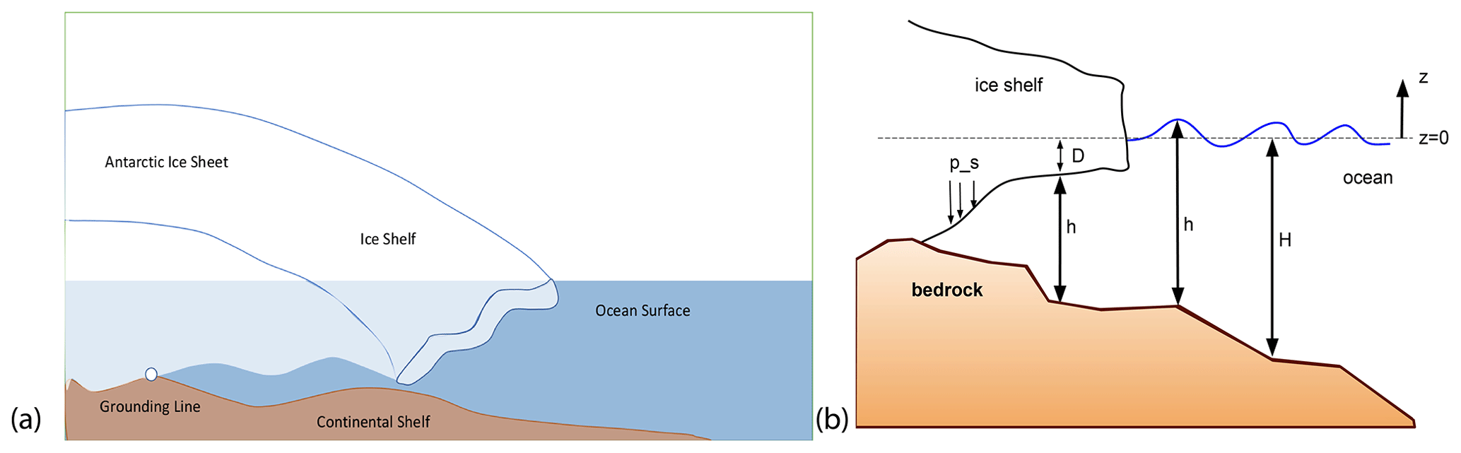
Figure 1(a) Schematic of ice shelf cavity. The grounding line (between the ice shelf and continental shelf) is marked with a white circle (b). Schematic showing the dynamic water thickness h, reference thickness H, ice draft D and surface pressure ps.
2.5 Ice shelf cavities and their connection to pressure
Within MPAS-Ocean the ocean domain is extended to include cavities under Antarctic ice shelves (Fig. 1, Jeong et al., 2020; Comeau et al., 2022). In our work, we do not study the dynamic ice-sheet–ocean coupling, so the ice-shelf–ocean interface is essentially static in time, adjusting only to the relatively small changes in dynamic pressure from the ocean. We use a constant density, salinity and temperature in our study and thus do not evolve these tracers separately. Since we have a single vertical ocean layer, we use a hydrostatic formulation for pressure with a linear dependency on the height of the vertical column (see Eq. 3). The implementation of ice shelf cavities require introducing an extra pressure term to Eq. (1) to account for the depression of sea surface height below the Antarctic ice sheet and above the continental shelf (see Fig. 1). This extra pressure ps represents the weight of floating ice shelves. The vertical coordinate below ice shelves in multi-layer MPAS-O is described in Comeau et al. (2022). For the single-layer version, the pressure is simply computed as ps=ρgD, where D is the ice shelf draft below the open-ocean sea surface datum and ρ is the density of the displaced water (Fig. 1b).
In this section we show that Eqs. (1)–(3), with the tidal forcing set to zero, reproduce known theoretical results for the ideal test cases: (a) the aquaplanet gravity wave test case and (b) Stommel's solution on a planar ocean basin. These two test cases are used to verify to operation of the single-layer shallow-water equations on the sphere, including the spatial discretization of the advection, Coriolis and pressure gradient terms and the time-stepping scheme.
An aquaplanet is a planet without any continents. If initialized with a Gaussian hump sea surface height test case, the Gaussian hump spreads at the speed of gravity waves in the ocean. The speed of gravity waves would be , where g is the acceleration due to gravity =9.8 m s−2 and H is the bottom depth of the ocean (here 1000 m). We have verified that our MPAS-Ocean simulations do indeed produce a gravity wave speed of (details in Sect. A in the Appendix).
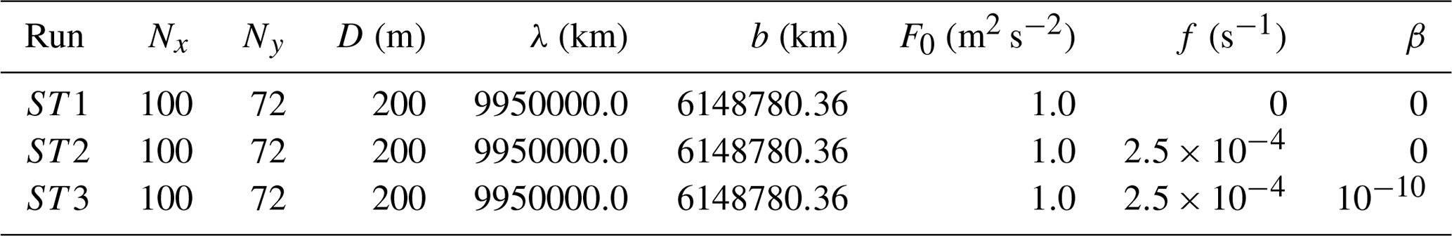
Next we check the Stommel solutions for a planar, flat-bottomed ocean basin. Stommel assumed a rectangular ocean with the origin of a Cartesian coordinate system at the southwest corner. The y axis points northward; the x axis is eastward. The shores of the ocean are at and . The values of these variables are listed in Table B1 in the Appendix. The ocean is regarded as a homogeneous layer of constant depth D when at rest. We observe that MPAS-Ocean simulation results agree very well with the analytical functions derived originally in Stommel (1948).
The system is initialized with a sinusoidal wind forcing as shown in the Appendix, Fig. B1b, and we simulate Eq. (1) for different values of Coriolis parameter. Below we show simulation results and also the corresponding analytical solutions, for a typical f plane test case, in which the Coriolis parameter is a constant (). The comparison of the MPAS-Ocean simulation results with the analytical results is shown in Fig. 2. A table with the system parameters is provided in Table B1 in the Appendix.
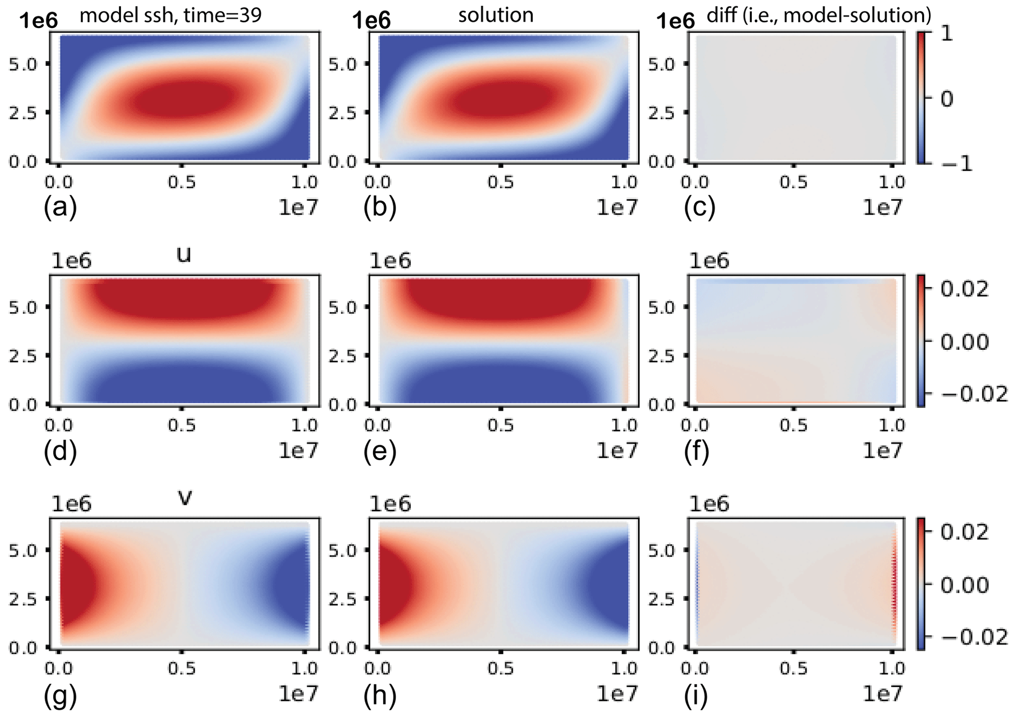
Figure 2Comparison of MPAS-Ocean results against theoretical predictions by Stommel (1948) for the f plane case: simulation (a, d, g); analytical solutions (b, e, h) and their difference (c, f, i) for the sea surface height (m), zonal velocity u and meridional velocity v (m s−1). Comparisons were made at 39 d, after the model reached an equilibrium solution. Horizontal axes are x and y (m).
4.1 Icosahedral mesh design
The horizontal meshes used throughout this study consist of quasi-uniform spherical centroidal Voronoi tessellations (SCVTs) based on a semi-structured icosahedral decomposition of the sphere. The coarsest grid is composed of 12 pentagonal Voronoi cells (primal grid) and an underlying dual triangular grid (dual grid). Refinements of this mesh are obtained by incremental bisection of the spherical triangle edges and application of an SCVT optimization procedure, which iteratively re-positions triangle vertices to lie at the center of mass of their associated Voronoi cells (Ju et al., 2011). The computational grids used in this study were generated using the JIGSAW unstructured meshing library (Engwirda, 2017). To facilitate mesh convergence analysis, we employ a set of four quasi-uniform, icosahedral-type meshes in this study, with between 7 and 10 levels of structured refinement. The icosahedron 7 configuration results in approximately 60 km global mesh spacing, while the highest-resolution icosahedron 10 configuration leads to approximately 8 km global resolution.
4.2 Variable-resolution mesh design
In addition to quasi-uniform icosahedral configurations, we also explore the use of unstructured, variable-resolution meshes to enhance the representation of coastal features and regions of high tidal dissipation through selective mesh refinement. Following previous work of Pringle et al. (2021) and consistent with Barton et al. (2023) and Brus et al. (2023), we employ a 45-to-5 km variable-resolution configuration with mesh spacing l(x) tailored to resolve barotropic wavelengths and sharp bathymetric gradients:
Here, lwav(x) and lslp(x) are barotropic tidal length-scale heuristics, with lwav increasing mesh resolution in shallow regions to resolve the wavelength of shallow-water dynamics and lslp increasing mesh resolution in areas of sharp bathymetry. βwav and βslp are tunable “mesh-spacing” parameters, set to and in this study. To control grid-scale noise, and are Gaussian-filtered () depths and gradients obtained from the GEBCO2021 bathymetry (GEBCO Compilation Group, 2020). l*(x) is a combined estimate of mesh spacing throughout the domain, clipping lwav, lslp to lmin=5 km and lmax=45 km globally. To control the gradation of the mesh overall, l*(x) is limited to enforce a sufficiently slow growth in length scale. We use in this study.
4.3 TPXO8 and tidal evaluation
To assess the accuracy of the implemented of tidal forcing, we compare the amplitude and phase of the tidal constituents obtained from the MPAS-Ocean simulations against those of data-assimilated TPXO8. We use a number of different meshes to assess their impact on the accuracy of our results. The meshes used are as follows: (1) a globally uniform icosahedron 7 mesh with a low resolution of 64 km; (2) a globally uniform icosahedron 8 mesh with a medium resolution 30 km; (3) a globally uniform icosahedron 9 mesh with a high resolution of 15 km; (4) a globally uniform icosahedron 10 mesh with an ultra-high resolution of 8 km; (5) a variable-resolution mesh ranging from 45 to 5 km. A single-layer global ocean configuration was initialized for each of the above meshes, and without any external wind forcing. An initial ramp-up time of 15 d was allowed for the tidal potential forcing, after which we observe a steady oscillation in the global mean kinetic energy. We compare the five major tidal constituents, of which three are semidiurnal, i.e., M2, S2, N2, and two are diurnal, i.e., K1, O1 as obtained from our MPAS-Ocean simulations against observational TPXO8 data. The mean harmonic decomposition of each tidal constituent over a period of 90 d was calculated from the MPAS-Ocean simulations. As a comparison metric, we choose the global complex root mean square error (RMSE) defined as follows:
where A is the tidal amplitude, θ is the phase lag, and the subscripts “o” and “m” refer to the observed and modeled values, respectively. The amplitude RMSE is defined as the limit of RMSE when θo=θm, i.e.,
The quantity RMSEA is weighted by the area dA of each cell. In our study, we perform the tidal analysis calculations for the M2 constituent of the tide only.
This section is organized in the following way: in Sect. 5.1 we show the tuning of the linear wave drag coefficient, χ, for different mesh resolutions. Thereafter, in the same section we show the impact of adding ice shelf cavities to the global tidal analysis results (in particular the amplitude and phase of the M2 tidal constituent) on the different meshes. In Sect. 5.2 we show the impact of adding inline SAL (see Barton et al., 2023, for details) to the MPAS-Ocean simulations on a variable-resolution mesh. In Sect. 5.3 we show comparisons of MPAS-Ocean simulation results against data obtained from tide gauge measurements. In Sect. 5.4 we compare the results from the different MPAS-Ocean meshes in bar chart plots. Finally, we wrap up our paper with some discussions and conclusions in Sect. 6.
Table 1RMSE values of the M2 tidal constituent, calculated for different simulations (Icos7n–VRis). “M2RMSE (global)” refers to the global RMSE value calculated without any ocean depth restrictions; “M2RMSE deep” refers to the global RMSE value calculated over ocean depths >1000 m. M2RMSER refers to RMSE values calculated between 66∘ N and 66∘ S and for ocean depths >1000 m. M2RMSESO refers to the RMSE values calculated over the Southern Ocean only, i.e., for latitudes south of 60∘ S; RMSETG refers to RMSE values obtained from the “Truth Pelagic” tide gauge database; RMSETGA refers to RMSE values obtained from the UHSLC tide gauge database along the Antarctic coastline.


Figure 3Tuning of the topographic wave drag coefficient χ for runs Icos8n (solid red with crosses) and Icos8is (dashed red with crosses), Icos9n (solid green with circles) and Icos9is (dashed green with circles), and Icos10n (solid blue with triangles) and Icos10is (dashed blue with triangles). See Table 1 for reference.
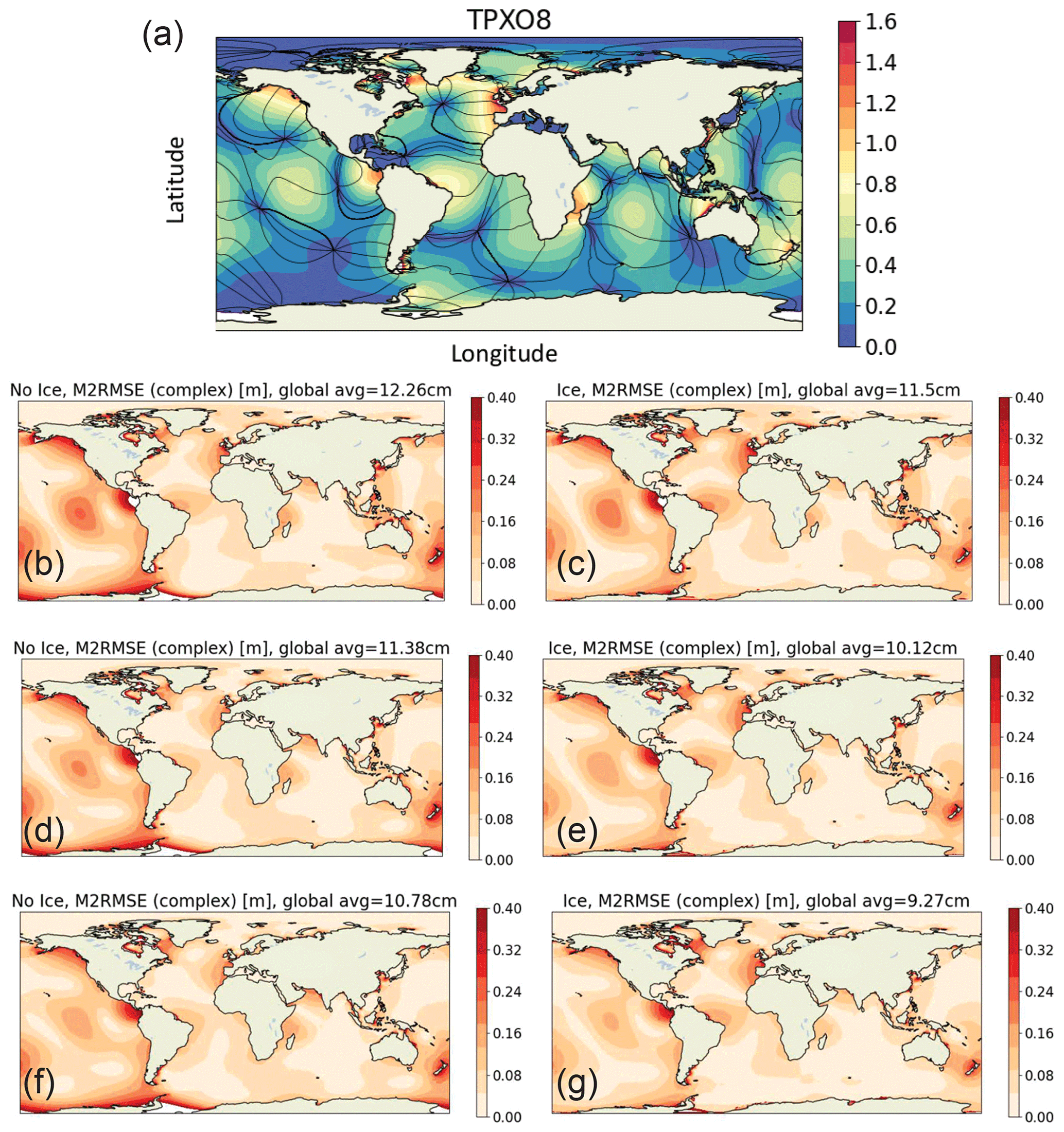
Figure 4Icosahedral global tidal simulation results: (a) reference TPXO8 re-analysis mean M2 amplitude (cm) with overlays of 90∘ phase contours. Complex RMSE (global, no depth or latitude restrictions) of M2 constituent for (b) Icos8n, (c) Icos8is, (d) Icos9n, (e) Icos9is, (f) Icos10n and (g) Icos10is.

Figure 5Difference in complex RMSE between Icos10n and Icos10is of (a) global and (b) South Polar projection. See Fig. 4f and g for reference.
5.1 TPXO8 comparisons and wave drag tuning
Due to the presence of a tunable parameter, χ, in the internal wave drag formulation, we carry out a series of simulations on each mesh configuration (icosahedron 8, 9 and 10) to find the optimum χ which gives the best agreement against TPXO8 data, i.e., the lowest value of RMSEA (see Sect. 4.3 for details). These simulations were carried out with and without adding ice shelf cavities. From these runs, we conclude that the optimum χ lies between 0.5 and 2.5 (see Fig. 3). The icosahedron N mesh is henceforth referred to as IcosNis and IcosNn for cases with and without ice shelf, respectively (here ). Note that the optimum value of χ for Icos9is (χ=1.08) and Icos9n (χ=1.44) are different. Similarly for the Icos10is and Icos10n meshes. In particular, the optimum value of χ is lower when there are ice shelf cavities in the simulation. This fact suggests that ice shelf cavities are responsible for the extra dissipation arising from a lower wave drag in the ocean. The lowest error obtained from these icosahedron mesh simulations is 0.088 m (Icos10is). It must be noted that we have used a scalar SAL term in these simulations.
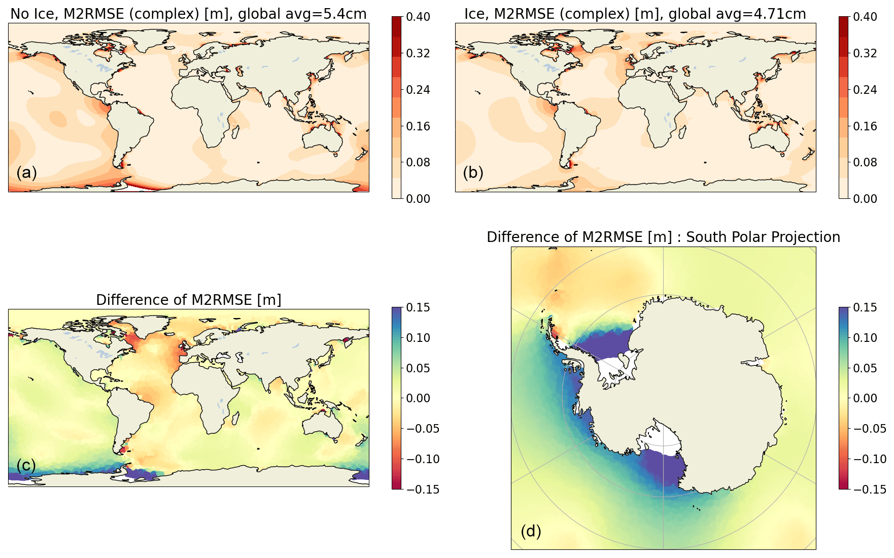
Figure 6M2 RMSE for the variable-resolution mesh and inline SAL (a) without and (b) with ice shelf cavities. The differences between plots (a) and (b) are shown in (c), along with a South Polar projection in (d).
The effects of tuning χ on the spatially varying RMSE of the M2 constituent, for Icos8n,is, Icos9n,is and Icos10n,is, are shown in Fig. 4b–g. Evidently, RMSEA improves when ice shelf cavities are added in the simulation. In particular, the global RMSEA decreases from 8.77 cm (Fig. 4b) to 8.3 cm (Fig. 4c) for the Icos8n,is meshes. The global RMSEA decreases from 8.0 cm (Fig. 4d) to 7.6 cm (Fig. 4e) for the Icos9n,is meshes and similarly from 7.9 cm (Fig. 4f) to 7.4 cm (Fig. 4g) for the Icos10n,is meshes.
As Fig. 4 shows, we perform two simulations for each mesh resolution: one with no Antarctic ice shelf cavities and one with Antarctic ice shelf cavities. As is apparent from a visual comparison of Fig. 4f and g, the Antarctic ice shelf cavities have the impact of reducing the errors along the Antarctic coastline. For a quantitative estimate of the reduction in errors, in Fig. 5a we show the difference in complex RMSE as obtained from Icos10n and Icos10is. Figure 5b shows a South Polar projection of the difference in RMSE between Icos10n and Icos10is.
5.2 Effect of ice shelf cavities and SAL
In this subsection we show that adding inline SAL (described in Sect. 2.4) improves the quality of MPAS-Ocean simulations substantially. In addition, the RMSE values show further improvement when we add Antarctic ice shelf cavities to our simulation. We use a variable-resolution horizontal mesh for this part of our work. We show the M2 RMSE plots for the MPAS-Ocean simulations without and with ice (VRn and VRis) in Fig. 6. The global deep water RMSE is 0.053 m for VR45–5n, which improves to 0.044 m (VR45–5is) when ice shelf cavities are added. The compounded effect of the inline SAL, ice shelf cavity forcing and the variable-resolution mesh results in the improvement in RMSE values for these two simulations. This is the lowest error achieved using the current stage of development of tides within MPAS-Ocean. As discussed later in this paper, state-of-the-art simulations by Schindelegger et al. (2018) and Shihora et al. (2022) have errors of 0.044 and 0.034 m, which are very close to the RMSE values in this study. We have shown that carefully tuned internal tide parameter, inline-SAL, ice shelves and a locally high-resolution mesh are all necessary to obtain accurate, high-quality tides simulations.
5.3 Tide gauge comparison
To further investigate the impact of ice shelf cavities on tidal dynamics, we compare the results of MPAS-Ocean to tide gauge datasets including the “ground truth” stations from the University of Hawaii Sea Level Center (UHSLC). The locations of these tide gauges are shown in Fig. 7e. Tidal harmonic data at these stations were consolidated by Pringle (2019). These data include directly provided tidal harmonics or those derived from using the Matlab Function for Unified Tidal Analysis and Prediction (UTIDE) (Codiga, 2011) on time level histories. Figure 7a–d show the model vs. tide gauge amplitudes and phases for runs VRn and VRis. These plots include gauges at latitudes south of 60∘ S. Figure 7a and b show scatterplots of the mean amplitude and phase of the tidal M2 constituent for the run VRn (i.e., no ice shelf cavity case). Similarly, Fig. 7c and d show scatterplots of the mean amplitude and phase of the tidal M2 constituent for the run VRis (i.e., with ice shelf cavity case). For the phase data, we shifted the values so that the phase differences were all within 180∘. The RMSE when comparing against the 21 UHSLC stations is 0.07 m for the variable-resolution mesh and 0.085 m for the 8 km quasi-uniform mesh (Table 1), which is consistent with the results seen from the TPXO8 comparison of 0.06 and 0.088 m, respectively, for the Southern Ocean.
We show values of correlation coefficient or the coefficient of determination R2 defined as follows:
Here x denotes M2 amplitude (in Fig. 7a and c) and M2 phase (in Fig. 7b and d) from MPAS-Ocean simulation data. y denotes M2 amplitude (in Fig. 7a and c) and M2 phase (in Fig. 7b and d) from tide gauge measurements. When there is no ice shelf in the simulation, the R2 values of the amplitude and phases are 0.8 and 0.83, respectively. Including ice shelf cavities increases the R2 values to 0.955 and 0.96, respectively. The ice shelf cavities, although static, provide an accurate boundary condition along the Antarctic coastline, and thus the tidal errors reduce appreciably in the Southern Ocean. The locations of the stations from which we record the tide gauge data are shown in Fig. 7e. Figure 7e shows a South Polar projection of the Southern Ocean, in particular, ocean between latitudes −90∘ and −60∘.
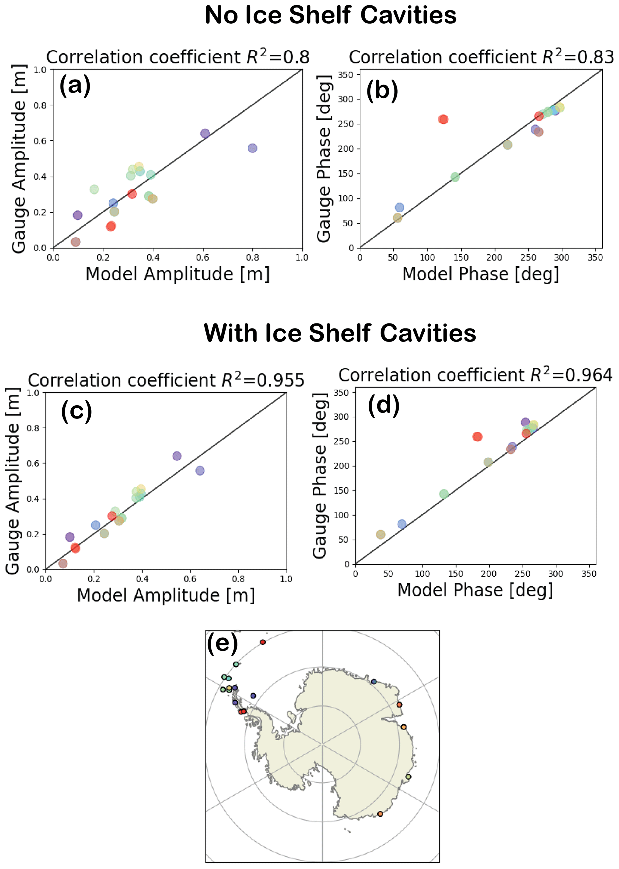
Figure 7Tide gauge comparison between the variable-resolution model simulation (horizontal axes) and observations (vertical axes) for M2 amplitude (a, c) and M2 phase (b, d), where the simulation is without ice shelves (VRn, a, b) and with ice shelves (VRis, c, d). These tide gauges are near the Antarctic coast and Drake Passage (e).
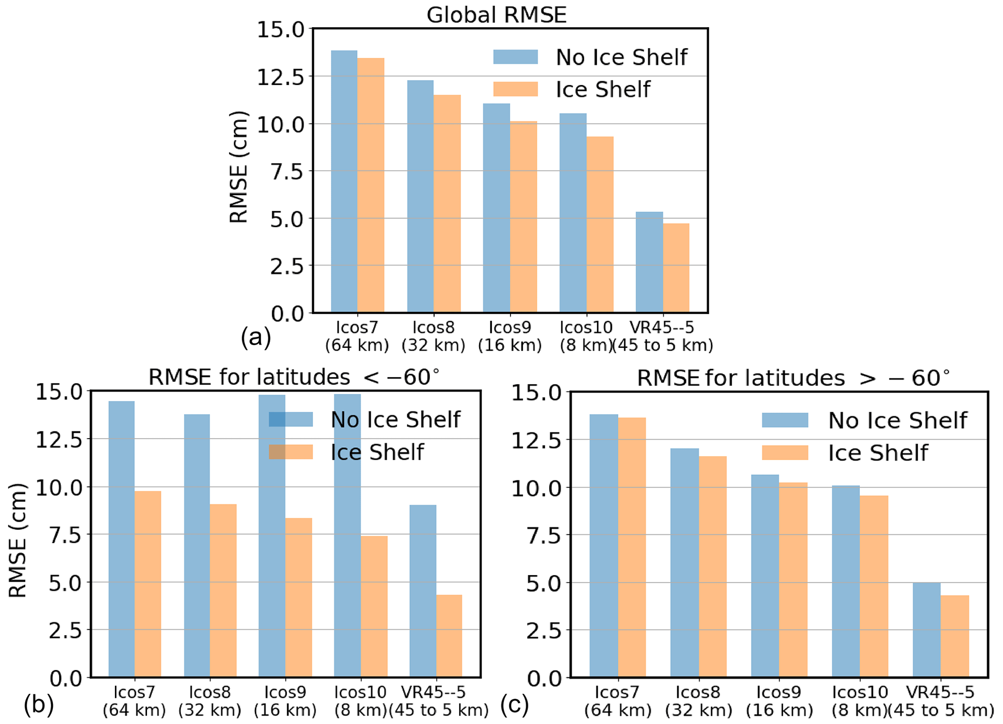
Figure 8Error for the icosahedron 7, 8, 9 and 10 meshes, with and without ice shelf cavities for (a) the global RMSE, (b) RMSE at latitudes ∘ and (c) RMSE at latitudes ∘.
5.4 Summary of all runs
Finally, Fig. 8 shows three bar chart plots exhibiting how ice shelf cavity forcing improves the RMSE in the different regions of the global ocean. In particular, the bar charts are in three categories: (a) the global ocean; (b) the Southern Ocean only (latitudes south of 60∘ S); (c) ocean for latitudes north of 60∘ S. Although the RMSE shows improvement with ice shelf cavities for all three categories, the strongest improvement is observed for the Southern Ocean (i.e., latitudes south of 60∘ S. This result further confirms that Antarctic ice shelf cavities are indeed required to accurately capture tides in an Earth system model.
The lowest error achieved is on the 45 to 5 km variable-resolutions mesh, with inline SAL and ice shelf cavities (VRis with a deep M2 RMSE of 0.044 m). As a point of comparison, Schindelegger et al. (2018) and Shihora et al. (2022) both included full inline SAL calculations in a barotropic tide model and found deep-ocean M2 RMSEs of 0.044 and 0.034 m, respectively. M2 RMSEs with the advanced circulation model ADCIRC were found to be 0.0287 m by Pringle et al. (2021), further lowered to 0.0194 m by Blakely et al. (2022). All four of the previous studies used a more optimized wave drag, and the last study implemented SAL by reading in SAL from a data-assimilated model. Stammer et al. (2014) includes a comparison of errors for various purely hydrodynamical, non-data assimilative models ranging from 0.0525–0.0776 m.
In this paper we have shown the effect of adding tides in a global ocean model and have explored the effects of drag and ice shelf cavities on global tides. We have computed the tidal analysis on meshes of different resolutions, in particular, the icosahedron meshes and also a variable-resolution mesh. In particular, we use a linear wave drag scheme, and show that a systematic tuning of the wave drag coefficient, χ, results in very accurate tides. We also found that the optimum value of χ is lower (see Fig. 3) when there are ice shelf cavities in the simulation, indicating the ice shelf cavities provide the extra dissipation. The detailed analysis of simulations with and without ice shelf cavities indicates that introducing static ice shelf cavities reduces the RMSEs appreciably along the Antarctic coastline (see Figs. 4 and 5). Finally, we have shown that using an inline self-attraction and loading term, along with ice shelf cavities, results in very accurate tides, as shown by comparison against observational TPXO8 data (see Fig. 6). Our results are further validated by comparison against tide gauge datasets (Fig. 7).
The computation of the full SAL term has been explored in detail in Barton et al. (2023) and Brus et al. (2023). In those works, the full SAL has been shown to predict better tides compared to a constant SAL coefficient. Although a detailed discussion of SAL is beyond the scope of this paper, we have shown (using one reference simulation) that inline SAL, along with ice shelf cavity forcing, reduces tidal errors appreciably.
It is clear from this work that ice shelf cavities improve tidal predictions. However, the ice shelf cavities have a fixed geometry in this work. This paper paves the way for future investigations of impacts of varying ice shelf cavity geometries on global tides. Since tides also affect the melting and freezing of ice shelf cavities as shown in Rosier et al. (2014), a two-way interaction between tides and ice shelf cavities will potentially improve tidal predictions. In this work we have primarily focused on tidal errors in the open ocean near the ice shelf cavities. However, a more detailed analysis of tides and tidal pressures near the grounding line is possible as shown by Begeman et al. (2020). Also, investigations of sea ice dynamics and floating ice shelves are expected to improve tidal errors (Sun et al., 2022; Lei et al., 2017). We would like to conduct more detailed investigations of these factors in a future effort.
The gravity wave speed on an aquaplanet domain, with no continents, is used to validate the barotropic model. If initialized with a Gaussian hump sea surface height test case (see Fig. A1a), the Gaussian hump spreads at the speed of gravity waves in the ocean (Fig. A1b–d represent the Gaussian profiles at times t=3.7, 6.1, 10 s, respectively). We calculate the velocity of propagation by tracking the position of a point at the edge of the circular patch in Fig. A1a–d. In particular, we track the maximum longitudinal coordinate where the sea surface height has a value 0.2 m. The speed of gravity waves would be , where g is the acceleration due to gravity =9.8 m s−2 and H is the bottom depth of the ocean (here 1000 m). Thus the gravity wave speed is ∼99.8 m s−1. The formula for gravity waves is the solution to the linear wave equation. Since we are running the MPAS-Ocean model with the nonlinear term, the speed will be slightly lower as shown in Fig. B1. The simulation parameters are shown in Table A1.
Table A1Parameters for an Aquaplanet test case simulated using MPAS-Ocean.

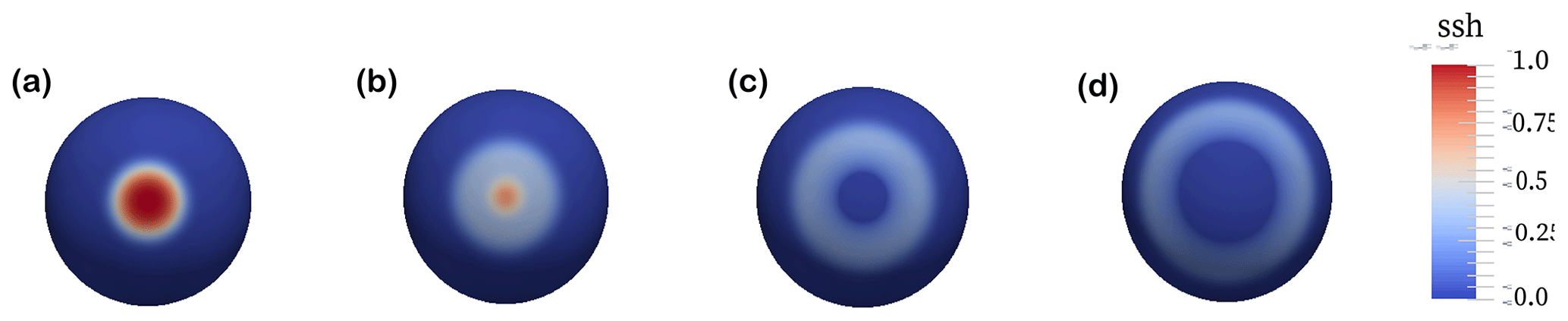
Figure A1Surface gravity wave on a sphere initiated by a Gaussian hump in sea surface height (ssh, m), at (a) t=0 s, (b) t=3.7 s, (c) t=6.1 s and (d) t=10 s.
Next we check the Stommel solutions for a planar, flat-bottomed ocean basin. Stommel assumed a rectangular ocean with the origin of a Cartesian coordinate system at the southwest corner. The y axis points northward; the x axis is eastward. The shores of the ocean are at and . The ocean is regarded as a homogeneous layer of constant depth D when at rest. Below we show the equations of motion according to Stommel (1948).
Here f is the Coriolis parameter, D is the bottom depth (200 m in our test case), h is the height above the sea surface, u is the x component of velocity, v is the y component of velocity and R is the Rayleigh friction coefficient.
Equations (B1)–(B2) are the steady-state Navier–Stokes equations. In Stommel (1948), Stommel derived analytical expressions for the sea surface height and the horizontal and vertical velocities for a planar domain and for different values of the Coriolis parameter f. The analytical solutions can be exactly verified against the MPAS-Ocean model solutions in the steady state, provided the domain configurations are the same as in Stommel (1948). Thus in MPAS, we choose a rectangular domain with the horizontal edges at xmin,xmax so that and the vertical edges at ymin and ymax so that .
Also, the coefficients in Eqs. (B1)–(B2) can be compared with those of Eq. (1). Rayleigh drag R in Eqs. (B1)–(B2) is [L][T]1, but the Rayleigh drag in MPAS is [T]−1. Thus R=0.02 m s−1 in Eqs. (B1)–(B2) corresponds to s−1 in MPAS, where H=200 m. The external force is provided by wind stress, which, for the sake of simplicity we consider to be a regular periodic function (Stommel, 1948). The wind force is given by . This simple functional form of the external force allows evaluation of analytical solution of Eqs. (B1)–(B2). The wind forcing amplitude is F0=1 N m2 in MPAS, which when divided by the density ρ gives the amplitude force per unit mass as m2 s−2. In Table B1 we give the different parameters, which are the same for the simulations in this section. We show a visualization of the wind forcing in the rectangular domain in Fig. B1.
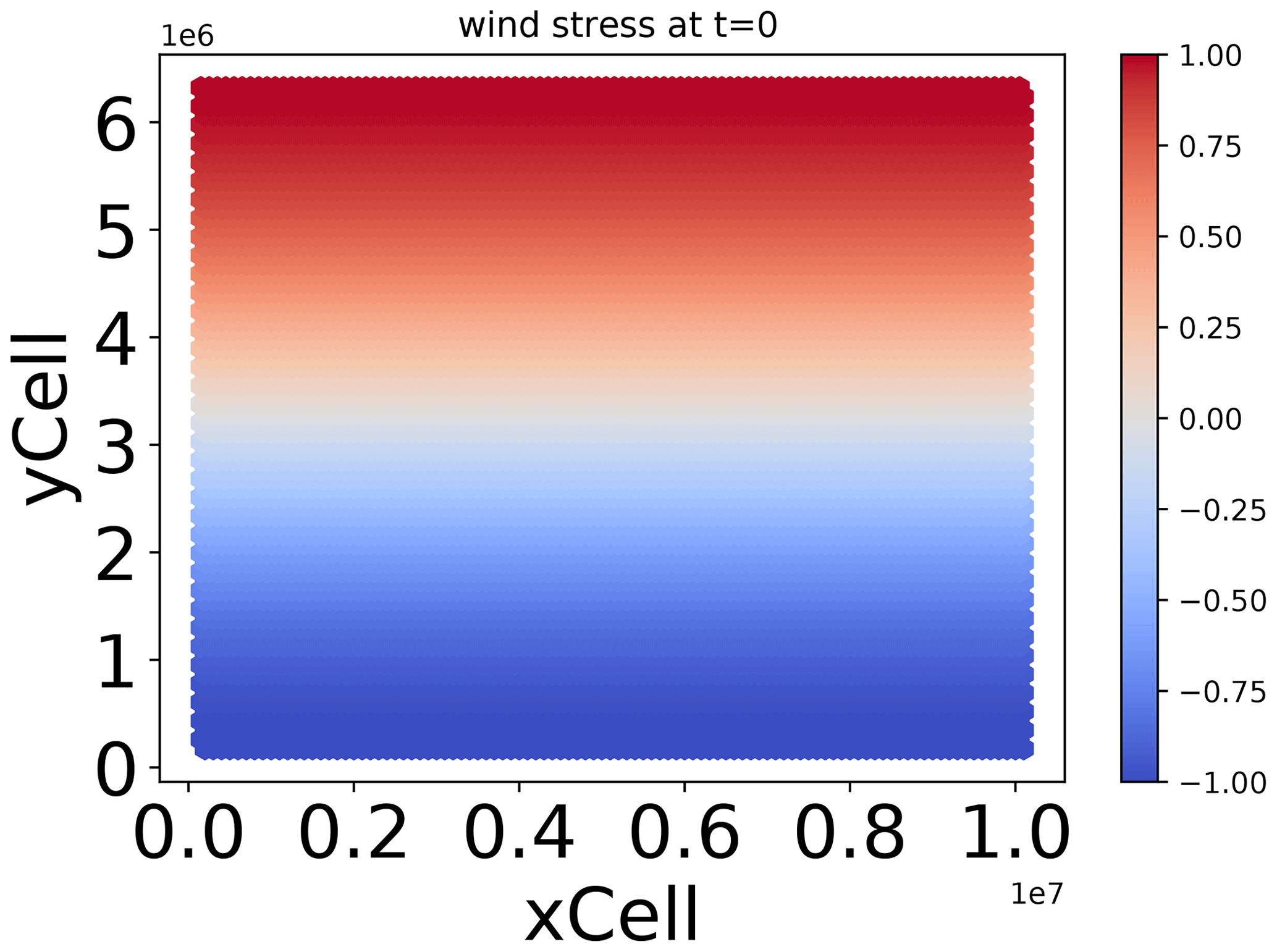
Table B1Simulation parameters for the Stommel test case on a planar ocean basin.
There is a wind forcing at t=0, with the initial condition shown in Fig. B1. We simulate Eq. (1) for different values of Coriolis parameter and list the cases below. We also provide the corresponding analytical solutions and compare the simulation results with the analytical results.
B1 Non-rotating ocean, f=0
If the Coriolis parameter is 0, the zonal and meridional velocities and the sea surface heights have the following analytical solutions in the steady state:
The corresponding comparisons are shown in Fig. 2.
B2 Ocean rotating at a constant angular velocity, i.e., f= constant
Here we have (see Table B1).
The x and y component of velocities and the sea surface height have the following expressions:
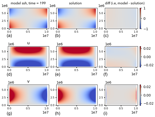
Figure B2Comparison of MPAS-Ocean results against theoretical predictions by Stommel (1948) for the non-rotating case (f=0): simulation (a, d, g); analytical solutions (b, e, h) and their difference (c, f, i) for the sea surface height (m), zonal velocity u and meridional velocity v (m s−1). Horizontal axes are x and y (m). Comparisons were made after the model reached an equilibrium solution.
B3 Rotating ocean:
Here, the Coriolis force varies linearly with latitude, i.e., , .
The x and y components of velocity and the sea surface height expressions are the following:
Code for the Energy Exascale Earth System Model (E3SM) used in this study is publicly available: https://github.com/E3SM-Project/E3SM/ (last access: 10 February 2023). A listing of the code and model configurations used in this work can be found in the following archive: https://doi.org/10.5281/zenodo.7084857 (Pal et al., 2022).
The dataset used in this study is located at https://doi.org/10.5281/zenodo.7084790 (Pal, 2023).
NP, KNB, MRP, DE and SRB prepared the paper, designed and implemented the coding upgrades into MPAS-Ocean, designed and performed the experiments, and conducted the tidal analysis. NP led the study, conducted the majority of simulations and analysis, and wrote the first draft of this paper. NP and MRP contributed to including the ice shelf cavities, topographic wave drag and bottom drag subroutines within MPAS-Ocean. DE contributed to the coding and development of the JIGSAW software integral to the horizontal mesh creation in this study. KNB and SRB and MRP contributed to the inline SAL calculation software. MRP and DE provided project oversight and code review. All authors participated in discussions to formulate the plan and provide feedback and reviewed and revised the text.
The contact author has declared that none of the authors has any competing interests.
Publisher's note: Copernicus Publications remains neutral with regard to jurisdictional claims in published maps and institutional affiliations.
This work was supported by the Earth System Model Development program area of the U.S. Department of Energy (DOE), Office of Science, Office of Biological and Environmental Research as part of the multi-program, collaborative Integrated Coastal Modeling (ICoM) project. Nairita Pal, Kristin N. Barton, Mark R. Petersen, Darren Engwirda and Brian K. Arbic acknowledge support from PNNL contract DE-AC05-76RL01830. Joannes J. Westerink and Damrongsak Wirasaet received support from the Joseph and Nona Ahearn endowment at the University of Notre Dame and by the U.S. DOE grant no. DOE DE-SC0021105. This research used resources of the National Energy Research Scientific Computing Center (NERSC), a U.S. DOE Office of Science User Facility located at Lawrence Berkeley National Laboratory, operated under contract no. DE-AC02-05CH11231, as well as resources provided by the Los Alamos National Laboratory Institutional Computing Program, which is supported by the U.S. DOE National Nuclear Security Administration under contract no. 89233218CNA000001
This research has been supported by the Biological and Environmental Research (grant no. DE-AC05-76RL01830).
This paper was edited by Rohitash Chandra and reviewed by two anonymous referees.
Accad, Y. and Pekeris, C. L.: Solution of the tidal equations for the M2 and S2 tides in the world oceans from a knowledge of the tidal potential alone, Philos. T. Roy. Soc. Lond. A, 290, 235–266, 1978. a, b
Arbic, B. K., Garner, S. T., Hallberg, R. W., and Simmons, H. L.: The accuracy of surface elevations in forward global barotropic and baroclinic tide models, Deep-Sea Res. Pt. II, 51, 3069–3101, 2004. a, b
Arbic, B. K., Alford, M. H., Ansong, J. K., Buijsman, M. C., Ciotti, R. B., Farrar, J. T., Hallberg, R. W., Henze, C. E., Hill, C. N., Luecke, C. A., Menemenlis, D., Metzger, E. J., Müller, M., Nelson, A. D., Nelson, B. C., Ngodock, H. E., Ponte, R. M., Richman, J. G., Savage, A. C., Scott, R. B., Shriver, J. F., Simmons, H. L., Souopgui, I., Timko, P. G., Wallcraft, A. J., Zamudio, L., and Zhao, Z.: A primer on global internal tide and internal gravity wave continuum modeling in HYCOM and MITgcm, New Frontiers in Operational Oceanography, edited by: Chassignet, E. P., Pascual, A., Tintoré, J., and Verron, J., GODAE OceanView, 307–392, https://doi.org/10.17125/gov2018.ch13, 2018. a
Barton, K. N., Pal, N., Brus, S. R., Roberts, A. F., Engwirda, D., Petersen, M. R., Arbic, B. K., Wirasaet, D., Westerink, J. J., and Schindelegger, M.: Global barotropic tide modeling using inline self‐attraction and loading in MPAS‐Ocean, J. Adv. Model. Earth Sy., 14, e2022MS003207, https://doi.org/10.1029/2022MS003207, 2023. a, b, c, d, e, f, g
Begeman, C. B., Tulaczyk, S., Padman, L., King, M., Siegfried, M. R., Hodson, T. O., and Fricker, H. A.: Tidal pressurization of the ocean cavity near an Antarctic ice shelf grounding line, J. Geophys. Res.-Oceans, 125, e2019JC015562, https://doi.org/10.1029/2019JC015562, 2020. a
Bell Jr., T. H.: Topographically generated internal waves in the open ocean, J. Geophys. Res., 80, 320–327, https://doi.org/10.1029/JC080i003p00320, 1975. a
Blakely, C. P., Ling, G., Pringle, W. J., Contreras, M. T., Wirasaet, D., Westerink, J. J., Moghimi, S., Seroka, G., Shi, L., Myers, E., Owensby, M., and Massey, C.: Dissipation and Bathymetric Sensitivities in an Unstructured Mesh Global Tidal Model, J. Geophys. Res.-Oceans, 127, e2021JC018178, https://doi.org/10.1029/2021JC018178, 2022. a, b
Brunt, K. M., Fricker, H. A., Padman, L., Scambos, T. A., and O’Neel, S.: Mapping the grounding zone of the Ross Ice Shelf, Antarctica, using ICESat laser altimetry, Ann. Glaciol., 51, 71–79, 2010. a
Brus, S. R., Barton, K. N., Pal, N., Roberts, A. F., Engwirda, D., Petersen, M. R., Arbic, B. K., Wirasaet, D., Westerink, J. J., and Schindelegger, M.: Scalable self attraction and loading calculations for unstructured ocean models, Ocean Model., 182, 102160, https://doi.org/10.1016/j.ocemod.2023.102160, 2023. a, b, c, d
Buijsman, M. C., Arbic, B. K., Green, J., Helber, R. W., Richman, J. G., Shriver, J. F., Timko, P., and Wallcraft, A.: Optimizing internal wave drag in a forward barotropic model with semidiurnal tides, Ocean Model., 85, 42–55, 2015. a, b, c
Buijsman, M. C., Ansong, J. K., Arbic, B. K., Richman, J. G., Shriver, J. F., Timko, P. G., Wallcraft, A. J., Whalen, C. B., and Zhao, Z.: Impact of parameterized internal wave drag on the semidiurnal energy balance in a global ocean circulation model, J. Phys. Oceanogr., 46, 1399–1419, 2016. a
Codiga, D. L.: Unified Tidal Analysis and Prediction Using the UTide Matlab Functions. Technical Report 2011-01. Graduate School of Oceanography, University of Rhode Island, Narragansett, RI. 59 pp., ftp://www.po.gso.uri.edu/pub/downloads/codiga/pubs/2011Codiga-UTide-Report.pdf (last access: 27 April 2022), 2011. a
Coleman, R.: Satellite altimetry and earth sciences: A handbook of techniques and applications, Eos Transactions American Geophysical Union, 82, 376–376, 2001. a
Comeau, D., Asay-Davis, X. S., Begeman, C. B., Hoffman, M. J., Lin, W., Petersen, M. R., Price, S. F., Roberts, A. F., Van Roekel, L. P., Veneziani, M., Wolfe, J. D., Fyke, J. G., Ringler, T. D., and Turner, A. K.: The DOE E3SM v1.2 Cryosphere Configuration: Description and Simulated Antarctic Ice-Shelf Basal Melting, J. Adv. Model. Earth Sy., 14, e2021MS002468, https://doi.org/10.1029/2021MS002468, 2022. a, b
De Kleermaeker, S., Verlaan, M., Mortlock, T., Rego, J. L., Apecechea, M. I., Yan, K., and Twigt, D.: Global-to-local scale storm surge modelling on tropical cyclone affected coasts, Australasian Coasts & Ports, 358–364, 2017. a
Egbert, G. and Ray, R.: Significant dissipation of tidal energy in the deep ocean inferred from satellite altimeter data, Nature, 405, 775–778, 2000. a
Egbert, G. D. and Ray, R. D.: Semi-diurnal and diurnal tidal dissipation from TOPEX/Poseidon altimetry, Geophys. Res. Lett., 30, 17, https://doi.org/10.1029/2003GL017676, 2003. a
Egbert, G. D., Ray, R. D., and Bills, B. G.: Numerical modeling of the global semidiurnal tide in the present day and in the last glacial maximum, J. Geophys. Res.-Oceans, 109, C3, https://doi.org/10.1029/2003JC001973, 2004. a, b, c, d
Engwirda, D.: JIGSAW-GEO (1.0): locally orthogonal staggered unstructured grid generation for general circulation modelling on the sphere, Geosci. Model Dev., 10, 2117–2140, https://doi.org/10.5194/gmd-10-2117-2017, 2017. a
GEBCO Compilation Group: GEBCO 2020 Grid, British Oceanographic Data Center [data set], https://doi.org/10.5285/a29c5465-b138-234d-e053-6c86abc040b9, 2020. a
Golaz, J.-C., Caldwell, P. M., Van Roekel, L. P., Petersen, M. R., Tang, Q., Wolfe, J. D., Abeshu, G., Anantharaj, V., Asay-Davis, X. S., Bader, D. C., Baldwin, S. A., Bisht, G., Bogenschutz, P. A., Branstetter, M., Brunke, M. A., Brus, S. R., Burrows, S. M., Cameron-Smith, P. J., Donahue, A. S., Deakin, M., Easter, R. C., Evans, K. J., Feng, Y., Flanner, M., Foucar, J. G., Fyke, J. G., Griffin, B. M., Hannay, C., Harrop, B. E., Hoffman, M. J., Hunke, E. C., Jacob, R. L., Jacobsen, D. W., Jeffery, N., Jones, P. W., Keen, N. D., Klein, S. A., Larson, V. E., Leung, L. R., Li, H.-Y., Lin, W., Lipscomb, W. H., Ma, P.-L., Mahajan, S., Maltrud, M. E., Mametjanov, A., McClean, J. L., McCoy, R. B., Neale, R. B., Price, S. F., Qian, Y., Rasch, P. J., Reeves Eyre, J. E. J., Riley, W. J., Ringler, T. D., Roberts, A. F., Roesler, E. L., Salinger, A. G., Shaheen, Z., Shi, X., Singh, B., Tang, J., Taylor, M. A., Thornton, P. E., Turner, A. K., Veneziani, M., Wan, H., Wang, H., Wang, S., Williams, D. N., Wolfram, P. J., Worley, P. H., Xie, S.,Yang, Y., Yoon, J.-H., Zelinka, M. D., Zender, C. S., Zeng, X., Zhang, C., Zhang, K., Zhang, Y., Zheng, X., Zhou, T., and Zhu, Q.: The DOE E3SM Coupled Model Version 1: Overview and Evaluation at Standard Resolution, J. Adv. Model. Earth Sy., 11, 2089–2129, https://doi.org/10.1029/2018MS001603, 2019. a
Gordeev, R., Kagan, B., and Polyakov, E.: The effects of loading and self-attraction on global ocean tides: the model and the results of a numerical experiment, J. Phys. Oceanogr., 7, 161–170, 1977. a
Green, J. M. and Nycander, J.: A comparison of tidal conversion parameterizations for tidal models, J. Phys. Oceanogr., 43, 104–119, 2013. a, b
Hendershott, M.: The effects of solid earth deformation on global ocean tides, Geophys. J. Int., 29, 389–402, 1972. a, b
Jacobs, S., Helmer, H., Doake, C., Jenkins, A., and Frolich, R.: Melting of ice shelves and the mass balance of Antarctica, J. Glaciol., 38, 375–387, 1992. a
Jayne, S. R. and St. Laurent, L. C.: Parameterizing tidal dissipation over rough topography, Geophys. Res. Lett., 28, 811–814, 2001. a, b, c, d, e, f, g
Jeong, H., Asay-Davis, X. S., Turner, A. K., Comeau, D. S., Price, S. F., Abernathey, R. P., Veneziani, M., Petersen, M. R., Hoffman, M. J., Mazloff, M. R., and Ringler, T. D.: Impacts of Ice-Shelf Melting on Water-Mass Transformation in the Southern Ocean from E3SM Simulations, J. Climate, 33, 5787–5807, https://doi.org/10.1175/JCLI-D-19-0683.1, 2020. a
Ju, L., Ringler, T., and Gunzburger, M.: Voronoi tessellations and their application to climate and global modeling, in: Numerical techniques for global atmospheric models, edited by: Lauritzen, P., Jablonowski, C., Taylor, M., and Nair, R., Springer, 313–342, https://doi.org/10.1007/978-3-642-11640-7_10, 2011. a
Kidder, D. L.: Facies models 4, Geoscience Canada, 38, 141–144, 2011. a
Knox, S., Windham-Myers, L., Anderson, F., Sturtevant, C., and Bergamaschi, B.: Direct and indirect effects of tides on ecosystem-scale CO2 exchange in a brackish tidal marsh in Northern California, J. Geophys. Res.-Biogeo., 123, 787–806, 2018. a
Le Provost, C., Genco, M., Lyard, F., Vincent, P., and Canceil, P.: Spectroscopy of the world ocean tides from a finite element hydrodynamic model, J. Geophys. Res.-Oceans, 99, 24777–24797, 1994. a
Ledwell, J., Montgomery, E., Polzin, K., St Laurent, L., Schmitt, R., and Toole, J.: Evidence for enhanced mixing over rough topography in the abyssal ocean, Nature, 403, 179–182, 2000. a
Lei, J., Li, F., Zhang, S., Ke, H., Zhang, Q., and Li, W.: Accuracy assessment of recent global ocean tide models around Antarctica, The International Archives of Photogrammetry, Remote Sensing and Spatial Information Sciences, 42, 1521, https://doi.org/10.3389/feart.2022.757821, 2017. a
Lyard, F., Lefevre, F., Letellier, T., and Francis, O.: Modelling the global ocean tides: modern insights from FES2004, Ocean Dynam., 56, 394–415, 2006. a
Melet, A., Nikurashin, M., Muller, C., Falahat, S., Nycander, J., Timko, P. G., Arbic, B. K., and Goff, J. A.: Internal tide generation by abyssal hills using analytical theory, J. Geophys. Res.-Oceans, 118, 6303–6318, 2013. a
Mellor, G. L. (Ed.): Introduction to physical oceanography, Springer, vol. 260, 1996. a
Munk, W.: Once again: once again – tidal friction, Prog. Oceanogr., 40, 7–35, 1997. a
Munk, W. and Wunsch, C.: Abyssal recipes II: Energetics of tidal and wind mixing, Deep-Sea Res. Pt. I, 45, 1977–2010, 1998. a, b
Munk, W. H.: Abyssal recipes, in: Deep Sea Research and Oceanographic Abstracts, Elsevier, 13, 707–730, 1966. a
Nikurashin, M. and Ferrari, R.: Global energy conversion rate from geostrophic flows into internal lee waves in the deep ocean, Geophys. Res. Lett., 38, 8, https://doi.org/10.1029/2011GL046576, 2011. a
Nycander, J.: Generation of internal waves in the deep ocean by tides, J. Geophys. Res.-Oceans, 110, C10, https://doi.org/10.1029/2004JC002487, 2005. a, b
Oey, L.-Y.: An OGCM with movable land–sea boundaries, Ocean Model., 13, 176–195, 2006. a, b
Padman, L., Siegfried, M. R., and Fricker, H. A.: Ocean tide influences on the Antarctic and Greenland ice sheets, Rev. Geophys., 56, 142–184, 2018. a
Pal, N.: Dataset for Barotropic tides in MPAS-Ocean (E3SM V2): impact of ice shelf cavities (GMD, 2023), Zenodo [data set], https://doi.org/10.5281/zenodo.7084790, 2023. a, b
Pal, N., Barton, K., Petersen, M., Brus, S. R., Engwirda, D., Arbic, B., Roberts, A. F., Westerink, J. J., and Wirasaet, D.: nPal/E3SM:MPAS-Ocean Tidal Dynamics in Presence of Ice Shelf Cavities, in a Barotropic Ocean, Zenodo, [code and data], https://doi.org/10.5281/zenodo.7084857, 2022. a
Petersen, M. R., Jacobsen, D. W., Ringler, T. D., Hecht, M. W., and Maltrud, M. E.: Evaluation of the arbitrary Lagrangian–Eulerian vertical coordinate method in the MPAS-Ocean model, Ocean Model., 86, 93–113, 2015. a
Petersen, M. R., Asay-Davis, X. S., Berres, A. S., Chen, Q., Feige, N., Hoffman, M. J., Jacobsen, D. W., Jones, P. W., Maltrud, M. E., Price, S. F., Ringler, T. D., Streletz, G. J., Turner, A. K., Van Roekel, L. P., Veneziani, M., Wolfe, J. D., Wolfram, P. J., and Woodring, J. L.: An Evaluation of the Ocean and Sea Ice Climate of E3SM Using MPAS and Interannual CORE-II Forcing, J. Adv. Model. Earth Sy., 11, 1438–1458, https://doi.org/10.1029/2018MS001373, 2019. a
Pringle, W.: Global Tide Gauge Database [data set], https://www.google.com/maps/d/u/0/viewer?mid=1yvnYoLUFS9kcB5LnJEdyxk2qz6g&ll=-3.81666561775622e-14,101.96502786483464&z=2, 2019. a
Pringle, W. J., Wirasaet, D., Roberts, K. J., and Westerink, J. J.: Global storm tide modeling with ADCIRC v55: unstructured mesh design and performance, Geosci. Model Dev., 14, 1125–1145, https://doi.org/10.5194/gmd-14-1125-2021, 2021. a, b
Ray, R.: Ocean self-attraction and loading in numerical tidal models, Marine Geodesy, 21, 181–192, 1998. a, b
Richter, O., Gwyther, D. E., King, M. A., and Galton-Fenzi, B. K.: The impact of tides on Antarctic ice shelf melting, The Cryosphere, 16, 1409–1429, https://doi.org/10.5194/tc-16-1409-2022, 2022. a
Ringler, T., Ju, L., and Gunzburger, M.: A multiresolution method for climate system modeling: Application of spherical centroidal Voronoi tessellations, Ocean Dynam., 58, 475–498, 2008. a
Ringler, T., Petersen, M., Higdon, R. L., Jacobsen, D., Jones, P. W., and Maltrud, M.: A multi-resolution approach to global ocean modeling, Ocean Model., 69, 211–232, 2013. a
Ringler, T. D., Thuburn, J., Klemp, J. B., and Skamarock, W. C.: A unified approach to energy conservation and potential vorticity dynamics for arbitrarily-structured C-grids, J. Computat. Phys., 229, 3065–3090, 2010. a, b
Rosier, S., Green, J., Scourse, J., and Winkelmann, R.: Modeling Antarctic tides in response to ice shelf thinning and retreat, J. Geophys. Res.-Oceans, 119, 87–97, 2014. a
Schindelegger, M., Green, J., Wilmes, S.-B., and Haigh, I. D.: Can we model the effect of observed sea level rise on tides?, J. Geophys. Res.-Oceans, 123, 4593–4609, 2018. a, b
Schlichting, H. and Gersten, K.: Boundary-layer theory, Springer, https://doi.org/10.1115/1.3641813, 2016. a
Schwiderski, E. W.: On charting global ocean tides, Rev. Geophys., 18, 243–268, 1980. a
Scott, R., Goff, J., Naveira Garabato, A., and Nurser, A.: Global rate and spectral characteristics of internal gravity wave generation by geostrophic flow over topography, J. Geophys. Res.-Oceans, 116, C9, https://doi.org/10.1029/2011JC007005, 2011. a
Shihora, L., Sulzbach, R., Dobslaw, H., and Thomas, M.: Self-attraction and loading feedback on ocean dynamics in both shallow water equations and primitive equations, Ocean Model., 169, 101914, https://doi.org/10.1016/j.ocemod.2021.101914, 2022. a, b
Stammer, D., Ray, R. D., Andersen, O. B., Arbic, B. K., Bosch, W., Carrère, L., Cheng, Y., Chinn, D. S., Dushaw, B. D., Egbert, G. D., Erofeeva, S. Y., Fok, H. S., Green, J. A. M., Griffiths, S., King, M. A., Lapin, V., Lemoine, F. G., Luthcke, S. B., Lyard, F., Morison, J., Müller, M., Padman, L., Richman, J. G., Shriver, J. F., Shum, C. K., Taguchi, E., and Yi, Y.: Accuracy assessment of global barotropic ocean tide models, Rev. Geophys., 52, 243–282, 2014. a
Stigebrandt, A.: Resistance to barotropic tidal flow in straits by baroclinic wave drag, J. Phys. Oceanogr., 29, 191–197, 1999. a
Stommel, H.: The westward intensification of wind-driven ocean currents, Eos, Transactions American Geophysical Union, 29, 202–206, 1948. a, b, c, d, e, f, g
Straneo, F., Heimbach, P., Sergienko, O., Hamilton, G., Catania, G.,Griffies, S., Hallberg, R., Jenkins, A., Joughin, I., Motyka, R., Pfeffer, W. T., Price, S. F., Rignot, E., Scambos, T., Truffer, M., and Vieli, A.: Challenges to understanding the dynamic response of Greenland's marine terminating glaciers to oceanic and atmospheric forcing, B. Am. Meteorol. Soc., 94, 1131–1144, 2013. a
Sun, W., Zhou, X., Zhou, D., and Sun, Y.: Advances and accuracy assessment of ocean tide models in the Antarctic Ocean, Front. Earth Sci., 10, 757821, https://doi.org/10.3389/feart.2022.757821, 2022. a
Taylor, G. I.: I. Tidal friction in the Irish Sea, Philos. T. Roy. Soc. Lond. A, 220, 1–33, 1920. a
Turner, J., Orr, A., Gudmundsson, G. H., Jenkins, A., Bingham, R. G., Hillenbrand, C.-D., and Bracegirdle, T. J.: Atmosphere-ocean-ice interactions in the Amundsen Sea embayment, West Antarctica, Rev. Geophys., 55, 235–276, 2017. a
Verfaillie, D., Pelletier, C., Goosse, H., Jourdain, N. C., Bull, C., Dalaiden, Q., Favier, V., Fichefet, T., and Wille, J. D.: The circum-Antarctic ice-shelves respond to a more positive Southern Annular Mode with regionally varied melting, Commun. Earth Environ., 3, 1–12, 2022. a
Vic, C., Naveira Garabato, A. C., Green, J., Waterhouse, A. F., Zhao, Z., Melet, A., de Lavergne, C., Buijsman, M. C., and Stephenson, G. R.: Deep-ocean mixing driven by small-scale internal tides, Nat. Commun., 10, 1–9, 2019. a
Von Kármán, T.: Mechanical similitude and turbulence, Tech. Mem., Report No. 611, Washington D.C., NACA, 1931. a
Wang, H., Xiang, L., Jia, L., Jiang, L., Wang, Z., Hu, B., and Gao, P.: Load Love numbers and Green's functions for elastic Earth models PREM, iasp91, ak135, and modified models with refined crustal structure from Crust 2.0, Comput. Geosci., 49, 190–199, 2012. a
Wang, P., Bernier, N. B., Thompson, K. R., and Kodaira, T.: Evaluation of a global total water level model in the presence of radiational S2 tide, Ocean Model., 168, 101893, https://doi.org/10.1016/j.ocemod.2021.101893, 2021. a
Warburton, K., Hewitt, D., and Neufeld, J.: Tidal grounding-line migration modulated by subglacial hydrology, Geophys. Res. Lett., 47, e2020GL089088, https://doi.org/10.1029/2020GL089088, 2020. a
Zaron, E. D. and DeCarvalho, R.: Identification and reduction of retracker-related noise in altimeter-derived sea surface height measurements, J. Atmos. Ocean. Tech., 33, 201–210, 2016. a
Zilberman, N., Becker, J., Merrifield, M., and Carter, G.: Model estimates of M 2 internal tide generation over Mid-Atlantic Ridge topography, J. Phys. Oceanogr., 39, 2635–2651, 2009. a
- Abstract
- Introduction
- Model formulation and equations
- Idealized experiments
- Global tidal dynamics: simulation details
- Results
- Conclusion
- Appendix A: Aquaplanet gravity wave test case
- Appendix B: Stommel basin test case
- Code availability
- Data availability
- Author contributions
- Competing interests
- Disclaimer
- Acknowledgements
- Financial support
- Review statement
- References