A new precipitation emulator (PREMU v1.0) for lower-complexity models

Precipitation is a crucial component of the global water cycle. Rainfall features (e.g., strength or frequency) strongly affect societal activities and are closely associated with the functioning of terrestrial ecosystems. Hence, predicting global and gridded precipitation under different emission scenarios is an essential output of climate change research, enabling a better understanding of future interactions between land biomes and climate change. Some current lower-complexity models (LCMs) are designed to emulate precipitation in a computationally effective way. However, for precipitation in particular, they are known to have large errors due to their simpler linear scaling of precipitation changes against global warming (e.g., IMOGEN; Zelazowski et al., 2018). Here, to reduce the errors in emulating precipitation, we provide a data-calibrated precipitation emulator (PREMU), offering a convenient and computationally effective way to estimate and represent precipitation well, as simulated by different Earth system models (ESMs) and under different user-prescribed emission scenarios. We construct the relationship between global and local precipitation and modes of global gridded temperature and find that the emulator shows good performance in predicting historically observed precipitation from Global Soil Wetness Project Phase 3 (GSWP3). The ESM-specific emulator also estimates well the simulated precipitation of nine ESMs and under four dissimilar future scenarios of atmospheric greenhouse gases (GHGs). Our ESM-specific emulator also reproduced well interannual fluctuations (R=0.82–0.93, p<0.001) of global land average precipitation (GLAP) simulated by the nine ESMs, as well as their trends and spatial patterns. The default configuration of our emulator only requires gridded temperature, also available from lower-complexity models such as IMOGEN (Zelazowski et al., 2018) and MESMER (Beusch et al., 2022; Nath et al., 2022), which themselves are calibrated against ESMs. Therefore, our precipitation emulator can be directly coupled within other LCMs, improving on, for instance, the current emulations of precipitation implicit in IMOGEN. The PREMU model has the opportunity to provide the driving conditions to model well the hydrological cycle, ecological processes and their interactions with climate change. Critically, the efficiency of LCMs allows them to make projections for many more potential future trajectories in atmospheric GHG concentrations than is possible with full ESMs due to the high computational requirement of the latter. By coupling with PREMU, LCMs will have the ability to emulate gridded precipitation; thus, they can be widely coupled with hydrological models or land surface models.

1 Introduction

Earth system models (ESMs) are the primary tools to study the impact of greenhouse gas (GHG) emissions on our climate, representing all the important Earth system processes (IPCC, 2013). However, there is a lack of sufficient computational power to run the most comprehensive, physically complete climate models for every application of interest (Nicholls et al., 2020) or for every potential future-emissions scenario. Thus, lower-complexity models (LCMs) are designed as the common approaches to improve computational efficiency in climate change research by focusing on the most impact-relevant variables (Gasser et al., 2017). By describing highly parameterized properties of the climate system, LCMs are many orders of magnitude faster than full-complexity ESMs (Nicholls et al., 2020). The simplest LCMs are energy balance models (EBMs) that use multiple parameterized numerical models to estimate the changes in greenhouse gas concentrations, radiative forcing and then global land–ocean average temperature under different emission scenarios (Meinshausen et al., 2011; Nicholls et al., 2020). However, such global “box” models do not simulate the spatial pattern of temperature. Some more complex LCMs, such as IMOGEN (Integrated Model Of Global Effects of climatic aNomalies; Zelazowski et al., 2018) and OSCAR (Gasser et al., 2017), additionally emulate the spatial pattern of temperature through the pattern-scaling method. Pattern scaling multiplies global temperature change by spatial patterns to give regional information (Zelazowski et al., 2018; Gasser et al., 2017; Huntingford et al., 2010; Tebaldi and Arblaster, 2014; Tebaldi and Knutti, 2018). Joint temperature and precipitation emulation by considering anthropogenic GHG forcing and large-scale modes of sea surface temperature (SST) variability has been proven possible (McKinnon and Deser, 2018, 2021). More recently, a spatially resolved emulator (the Modular Earth System Model Emulator with spatially Resolved output, MESMER) solely requiring global mean temperature (GMT), e.g., by coupling to the emission-driven LCM MAGICC (Model for the Assessment of Greenhouse Gas Induced Climate Change), to then generate annual temperature fields has been developed (Beusch et al., 2022). Other than temperature, however, it is still a challenge for LCMs to simulate well other climate variables such as precipitation under different emission scenarios (Gasser et al., 2017).

Precipitation has high spatio-temporal variability and is affected by atmospheric dynamics and interannual modes of variability (Li et al., 2021; Tsanis and Tapoglou, 2019), making representing it within traditional LCM approaches difficult. Thus, only two LCMs (IMOGEN and OSCAR) have tried to emulate precipitation but with poor skill (Zelazowski et al., 2018; Gasser et al., 2017). IMOGEN emulates the gridded precipitation based on the regression relationship (by month and location) between gridded precipitation and global land average temperature (Zelazowski et al., 2018). OSCAR constructs the emulator by establishing a relationship between global average precipitation and global average temperature and radiative forcing, from which a pattern-scaling method is used to deduce the gridded precipitation (Gasser et al., 2017). Nevertheless, the gridded precipitation estimated by the simple linear method is not fully reliable in either IMOGEN or OSCAR; the gridded precipitation predicted by IMOGEN explains less than 20 % of the variance of seasonal precipitation in most regions (Zelazowski et al., 2018), and OSCAR cannot capture the interannual variations of regional precipitation across the globe at all (Gasser et al., 2017). This may be because (1) the global average temperature could not fully characterize local temperature and moisture recycling (Prein et al., 2017) and large-scale circulation (Shepherd, 2014; Fereday et al., 2018; Heinze-Deml et al., 2021), and/or (2) there is at any given location a nonlinear relationship between local rainfall features and global warming (Allen and Ingram, 2002; Collins et al., 2013; Chadwick and Good, 2013). Hence, models such as IMOGEN, which rely on linear pattern scaling, by definition cannot fully capture expected future precipitation changes. Nevertheless, precipitation is a crucial component of the water cycle (Eltahir and Bras, 1996; Trenberth et al., 2003; Sun et al., 2018), has key societal implications and is closely associated with the functioning of terrestrial ecosystems. Accurately emulating precipitation change is necessary to determine the climate response to different emission scenarios and to understand feedbacks to global warming via rainfall-dependent vegetation's net primary productivity (Gasser et al., 2017).

Previous studies have confirmed the important impact of ocean–atmosphere oscillations on interannual and interdecadal variations of regional precipitation (e.g., Li et al., 2021; Tsanis and Tapoglou, 2019; Dai, 2013). As such, our noted changes in gridded surface air temperature likely contain information about sea surface temperature and ocean–atmosphere oscillations in addition to information on the background global land average temperature. To this end, we proposed a computationally efficient precipitation emulator (PREMU), which uses gridded temperature data as independent forcing variables to reconstruct the gridded precipitation. We have designed the presented emulator such that it can act as, for instance, an enhanced precipitation module for the OSCAR and IMOGEN models. Alternatively, PREMU could be coupled directly with the MAGICC-MESMER and MESMER-M emulators. When coupling with other LCMs, tracing gridded precipitation under novel trajectories for GHGs will be possible. In Sects. 2 and 3, we described the datasets (both measurement- and ESM-based) and the methods to construct the driving-data-specific emulator for historical observation and each ESM in detail. We illustrated the emulator's ability to emulate the historical and future precipitation in Sect. 4. Finally, Sect. 5 discusses the strengths and caveats of our emulator.

2 Data

In the analysis, we tested the performance of PREMU for both historical periods (1901–2016) and future periods (2015–2100). For historical periods, we used different time periods of observation data for calibration (1901–1950) and validation (1951–2016), while for the future, we used ESM data under different emission scenarios for calibration (SSP5–8.5) and validation (SSP1–2.6, SSP2–4.5 and SSP3–7.0).

2.1 Observation datasets

To verify the ability to predict historical precipitation using the emulator proposed in this study, we first demonstrated the applicability of the emulator to observational data provided by the Global Soil Wetness Project Phase 3 (GSWP3; Kim, 2017). The GSWP3 dataset is based on the 20th Century Reanalysis (20CR) version 2c (Compo et al., 2011) and has precipitation fields at a resolution of 2^∘ × 2^∘. The GSWP3 data are dynamically downscaled using spectral nudging and bias correction from the Global Precipitation Climatology Project and Climate Research Unit (Humphrey and Gudmundsson, 2019). This approach successfully keeps the low-frequency signal of the two original reanalysis products yet also provides additional high-frequency signals that were lacking in previous products but are essential for investigating extreme events (Kim, 2017). GSWP3 also provides the other seven climate variables, including 2 m air temperature (T_air), specific humidity, surface downwelling long-wave radiation, surface downwelling short-wave radiation, surface air pressure and near-surface wind speed at a 0.5^∘ × 0.5^∘ spatial resolution from years 1901 to 2016. Here, with an emphasis on precipitation, we used T_air and precipitation from GSWP3 from the period 1901 to 1950 to calibrate the emulator and from 1951 to 2016 to verify the emulator's performance in predicting historical precipitation.

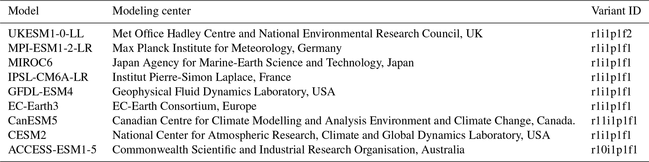
Table 1 List of the nine employed CMIP6 models and the modeling groups that provided them.

2.2 Earth system model data

To evaluate the emulator's performance in estimating future precipitation, we additionally used monthly precipitation and 2 m T_air for years 2015 to 2100 from nine ESMs operated under four shared socioeconomic pathways (SSPs; SSP1–2.6, SSP2–4.5, SSP3–7.0, and SSP5–8.5; O'Neill et al., 2016). These ESMs are included in the sixth phase of the Coupled Model Intercomparison Project (CMIP6; Table 1). The SSP5–8.5 scenario represents the largest future change of GHG concentrations compared to the other three SSPs (Hausfather and Peters, 2020) and so is associated with the largest variation in precipitation and T_air changes. Hence, we used the precipitation and T_air from SSP5–8.5 to calibrate the emulator and the other three scenarios to verify the emulator's performance at reproducing ESMs. However, note that the emulator based on this extreme-warming scenario (SSP5–8.5) may not produce well the precipitation patterns of cooler scenarios (e.g., SSP1–2.6) due to the nonlinear response of the atmosphere to warming. We discuss this further in Sect. 5. In addition, in view of the different responses of precipitation to the changes of T_air in different ESMs, we constructed the emulator for each ESM respectively. For comparison between different models, the precipitation and T_air from all nine ESMs are re-gridded to the resolution of 2.5^∘ × 2.5^∘ using the first-order conservative remapping technique (Jones, 1999). As there remains substantial error and uncertainty in gridded precipitation data, we retained only a first-order regridding method for precipitation or T_air (we note that second-order calculations have been used by others; Brunner et al., 2020).

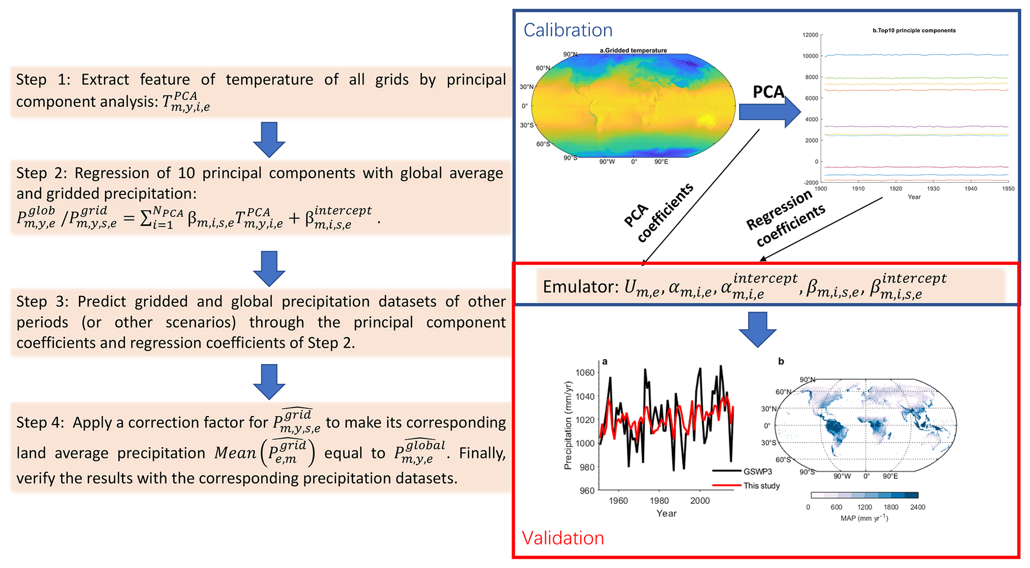
Figure 1 Illustration of the precipitation emulator driven by the gridded temperature. Step 1 is to extract the features of gridded temperature through principal-component analysis. In Step 2, we construct the parameters of the emulator by regression of GLAP or gridded precipitation and the principal components of gridded temperature. Then we use the emulator to predict the precipitation for the validation period or scenario in Step 3. Finally, we calibrate the precipitation and verify the results with precipitation from GSWP3 and ESMs. Here, $T_{e,m}^{\mathrm{PCA}}(y,i)$ is the principal components extracted by PCA. $P_{e,m}^{\mathrm{global}}\left(y\right)$ is the GLAP, and $P_{e,m}^{\mathrm{grid}}(k,y)$ is the precipitation of a given grid k. ${\mathit{\alpha }}_{e,m}\left(i\right)/{\mathit{\beta }}_{e,m}(k,i)$ represents the coefficients of each principal component of temperature in relation to global and/or gridded precipitation, and ${\mathit{\alpha }}_{e,m}^{\mathrm{intercept}}\left(i\right)/{\mathit{\beta }}_{e,m}^{\mathrm{intercept}}(k,i)$ is the intercept term. $U_{e,m}^{\mathrm{Spatial}}(k,i)$ is the PCA coefficients. Note that the gridded temperature from GSWP3 has an area-weighted average of 2.5^∘ × 2.5^∘ before PCA.

3 Methods

3.1 General approach

Given the relatively poor linear relationship between global and/or gridded (i.e., local) precipitation and global land mean temperature (as noted in Zelazowski et al., 2018), we try to build a new emulator for precipitation. We still search for a relationship between precipitation change and some function of gridded T_air (Fig. 1), albeit one that is more complex than simply linear in relation to global temperature. Since precipitation is also controlled not only by local temperature (Zhou et al., 2020), we seek links to features of T_air from all grid cells. There are 10 368 grid boxes considered at a common 2.5^∘ × 2.5^∘ resolution, which we used for both historical observations and future ESMs after remapping the latter. It is these T_air data and model simulations that we used across the globe to predict precipitation variation.

In this section, we set out underlying methods for our emulation of local precipitation by the principal-component-regression (PCR) approach, based on relating it to the dominant modes of variability of temperature. PCR is a type of regression analysis, which considers the orthogonal principal components as independent variables. As a method that can be used to overcome the problem of multi-linearity in predictor variables, the PCR technique is widely used in forecasting seasonal precipitation (Kim et al., 2017) and reconstructing the climatic modes of variability (Jones et al., 2009; Michel et al., 2020). These authors find the PCR method performs remarkably well, and the method is explained in detail in Chapter 13 of Storch and Zwiers (2011). As might be expected, therefore, our starting point is to derive the principal components of global gridded temperature. We followed the standard procedure of principal-component analysis (PCA), as used in climate research (e.g., Yan et al., 2020; Singh, 2006; Jiang et al., 2020), that consists of a set of time-invariant spatial patterns multiplied by time series of coefficients. PCA notation can vary between users, but for simplicity, we will simply refer to PCA “spatial patterns” (each of which has the dimensions of the spatial grid or, alternatively, an array of one dimension with 10 368 points) and PCA “time series”, which multiply the patterns. These time series, derived for each month, contain values applicable for each year – so, for instance, fitting to years 1901–1950 implies that they will have 50 numbers. As precipitation may be influenced by the temperature of the previous months via large-scale circulation (e.g., the lag effects of the El Niño–Southern Oscillation (ENSO) on regional precipitation; Li et al., 2011; Lu et al., 2019; Efthymiadis et al., 2007), we used the average T_air of 3 months (month of interest plus the previous two months) to apply PCA. In addition, considering that ESMs may underrepresent the effects of topography and aerosols on modeled precipitation (Samset et al., 2016; Yang et al., 2021), we calibrated the emulator for the historical period and future period separately. For the estimates of future change, we used precipitation and T_air from the SSP5–8.5 scenario of greenhouse gas increases to calibrate the ESM-specific emulator. We selected this scenario due to its representation of the most extreme changes in T_air amongst SSPs (O'Neill et al., 2016).

Table 2 List of index labels and variable symbols in the calibration.

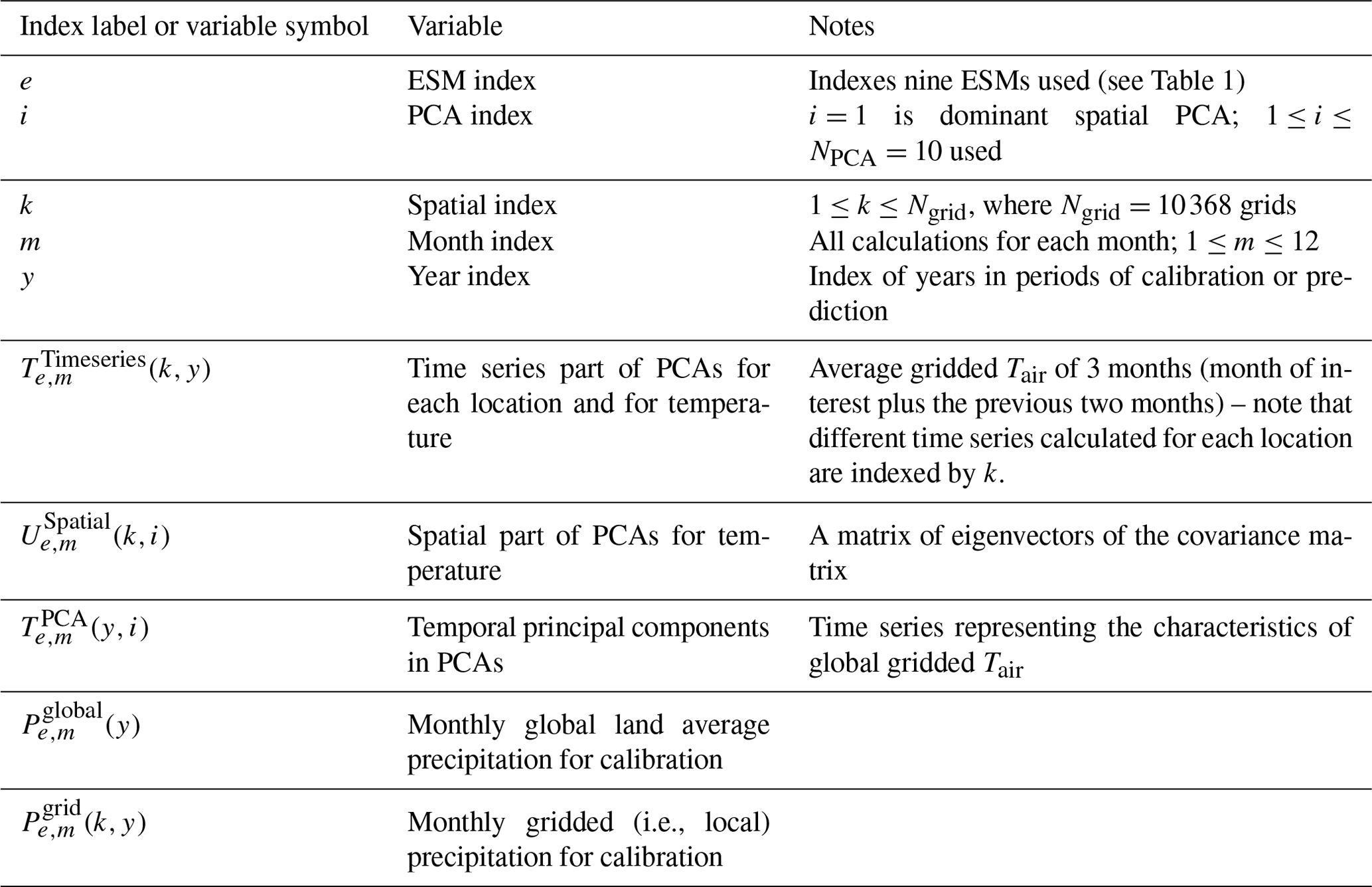
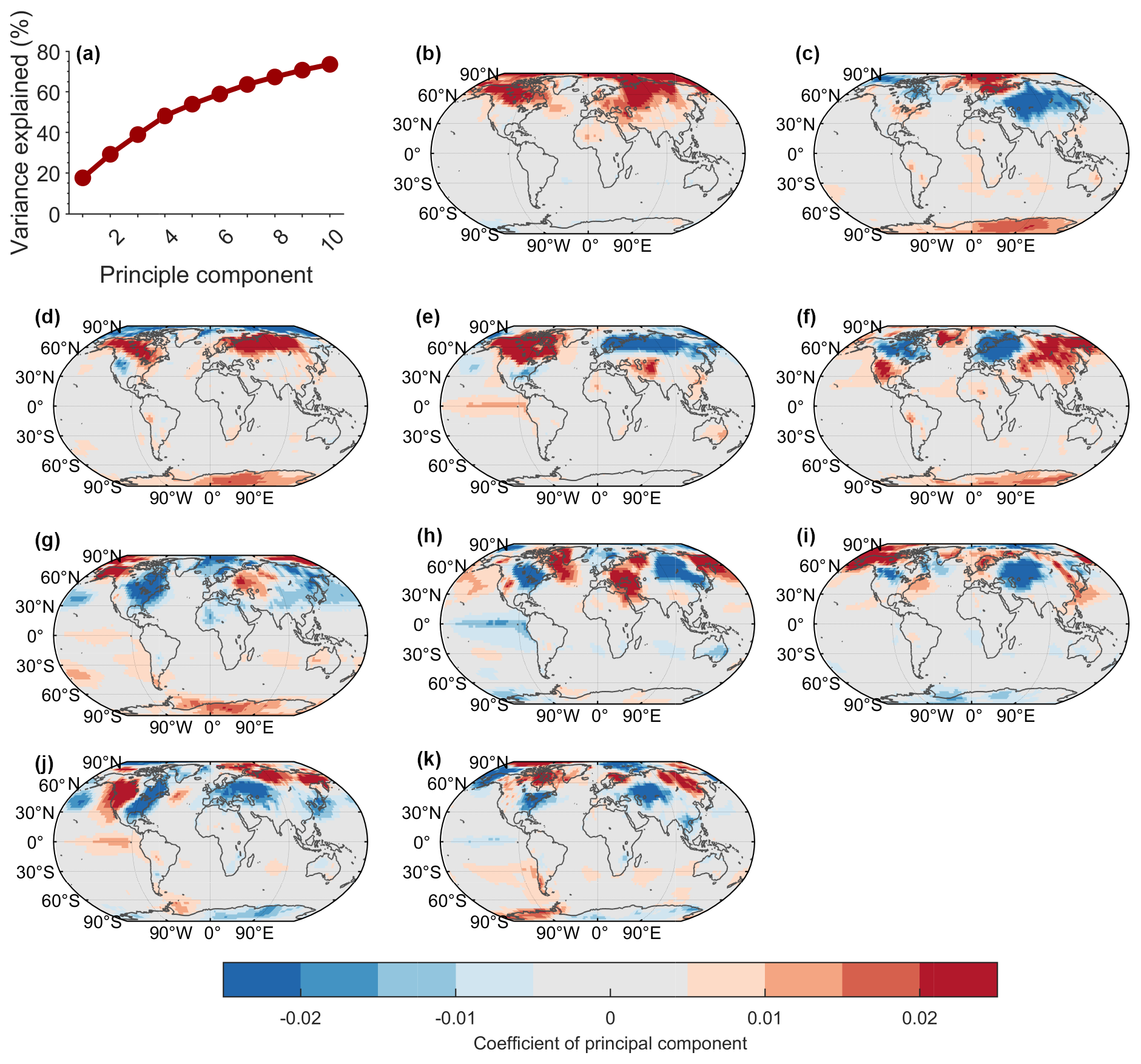
Figure 2 The corresponding results from the PCA of the gridded temperature in January between 1901 and 1950 from GSWP3: (a) the cumulative variance explanation rate of the top 10 principal components; (b–k) coefficients of the top 10 principal components (corresponding to $U_{e,m}^{\mathrm{Spatial}}\left(:,i\right)$, i=1–10).

3.2 Framework for PREMU

3.2.1 Calibration

We set out in Table 2 below our notation for indices and variable quantities.

Our use of the standard definition of PCAs (sum of patterns × time series) implies that the estimate of the principal components is given by the spatial pattern of principal-component coefficients $U_{e,m}^{\mathrm{Spatial}}(k,i)$ multiplied by the time series of 3 months' average gridded temperature. The choice of the 3-month average T_air as an independent variable is robust, with further details illustrated in Sect. 5. The PCA component coefficients, $U_{e,m}^{\mathrm{Spatial}}(k,i)$, are the combination of eigenvectors of the covariance matrix of the anomalies of the gridded 3-month average T_air. However, unlike many limited-area applications that derive a single time series (to multiply each PCA; Rahaman et al., 2019), we instead determined a time series for each location, and hence, $T_{e,m}^{\mathrm{Timeseries}}(k,y)$ has a k dependency. We then summed over all locations k, and this gives a global annual time series (for each ESM e, month m, year y and PCA i) of

$$\begin{array}{}\text{(1)}& T_{e,m}^{\mathrm{PCA}}\left(y,i\right)={\sum }_{k=\mathrm{1}}^{N_{\mathrm{grid}}}{U}_{e,m}^{\mathrm{Spatial}}\left(k,i\right)\cdot T_{e,m}^{\mathrm{Timeseries}}\left(k,y\right).\end{array}$$

Using T_air for years 1901–1950 from the GSWP3 gridded dataset and for the period 2015–2100 from the nine ESMs forced under the SSP5–8.5 scenario, we determined the principal-component coefficient matrix $U_{e,m}^{\mathrm{Spatial}}$ for each month m and the ESM e (or GWSP3) independently. We employed Eq. (1), and the top 10 principal components (i=1, …, 10) were used in this study – these describe more than 70 % of gridded temperature information (i.e., variation) across the globe (Figs. 2 and S1–S3). The stability of the component coefficients $U_{e,m}^{\mathrm{Spatial}}(k,i)$ of the top 10 PCs between different scenarios is discussed in Sect. 5. Otherwise, we found that the 15 ocean–atmosphere climate indices can be well reconstructed by multilinear regression of the top 10 principal components $T_{e,m}^{\mathrm{PCA}}\left(y,\mathrm{1}:\mathrm{10}\right)$ (Fig. S4). This suggests that the principal components of gridded temperature likely additionally contain information about sea surface temperature and ocean–atmosphere oscillations, which have great impacts on interannual and interdecadal variations of regional precipitation.

Having established the temperature principal components via the form presented in Eq. (1), we then mapped these onto precipitation both globally and locally. Our mapping is via a standard regression based on 50 data points (i.e., years 1901–1950, or 86 data points in ESMs for years 2015–2100). The regression has 40 degrees of freedom due to our selection of 10 PCAs, and this relationship links the time series of monthly gridded precipitation from the GSWP3 dataset (or the nine ESMs) and the 10 principal components of gridded temperature for each month of the 12 months of the year (January to December). This regression (for each ESM e, month m, grid k and year y) is constructed as follows:

$$\begin{array}{}\text{(2)}& P_{e,m}^{\mathrm{grid}}(k,y)={\sum }_{i=\mathrm{1}}^{N_{\mathrm{PCA}}}{\mathit{\beta }}_{e,m}\left(k,i\right)\cdot T_{e,m}^{\mathrm{PCA}}(y,i)+{\mathit{\beta }}_{e,m}^{\mathrm{intercept}}(k,i),\end{array}$$

where $P_{e,m}^{\mathrm{grid}}(k,y)$ is the precipitation at a specific cell k. Variable β_e,m represents the regression coefficient of each principal component, and ${\mathit{\beta }}_{e,m}^{\mathrm{intercept}}$ is the intercept term; these are derived from linear regressions by the least-squares method using the calibration time series. To provide the reliable estimation of global monthly precipitation $\widehat{P_{e,m}^{\mathrm{global}}\left(y\right)}$, we constructed the regression relationship between global land average precipitation (GLAP) and the 10 individual principal components separately, following Eq. (2).

Table 3 List of variable symbols in the validation.

3.2.2 Generating emulations using PREMU

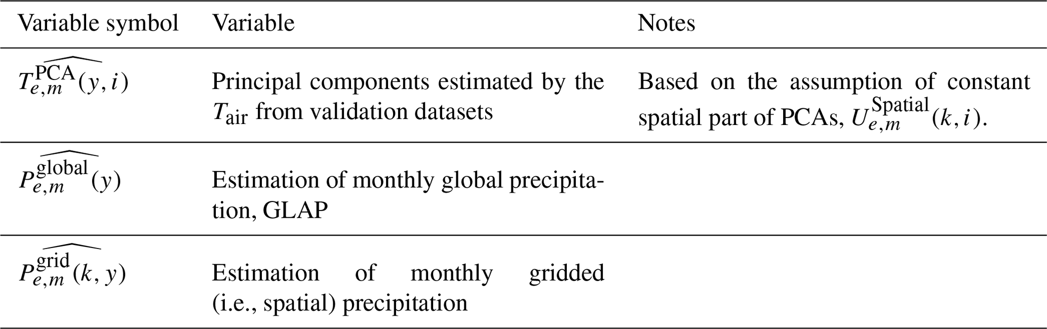
For validation, we set out in Table 3 below the variables that we estimated with our methodology. The “overhat” notation represents an estimated quantity. We first recalled that we fitted our PCA-based framework to historical temperature and precipitation data for the period 1901–1950 and to ESMs for the SSP5–8.5 future atmospheric GHG concentration scenario. Based on the principal-component coefficients extracted using these calibration datasets, we then estimated the $\widehat{T_{e,m}^{\mathrm{PCA}}(y,i)}$ using Eq. (1), using T_air from GSWP3 for 1951–2016 and, for 2015–2100, using T_air from each ESM independently under the other three SSPs. Then we estimated the $\widehat{P_{e,m}^{\mathrm{global}}\left(y\right)}$ and $\widehat{P_{e,m}^{\mathrm{grid}}(s,y)}$ individually by means of the $\widehat{T_{e,m}^{\mathrm{PCA}}(y,i)}$ and our fitted-regression coefficients in Eq. (2).

3.3 Validation

Before evaluating the performance of PREMU, we found a slight difference in GLAP between $\widehat{P_{e,m}^{\mathrm{global}}}$ and the spatial average of $\widehat{P_{e,m}^{\mathrm{grid}}}$, brought about by setting negative numbers of $\widehat{P_{e,m}^{\mathrm{grid}}}$ to zero at some grid points. Thus, as a final component to our calculations, we scale $\widehat{P_{e,m}^{\mathrm{grid}}}$ by the ratio of $\widehat{P_{e,m}^{\mathrm{global}}}$ and the monthly GLAP from the average the over grid points as area-averaged $\widehat{P_{e,m}^{\mathrm{grid}}}$, i.e., with the following equation:

$$\begin{array}{}\text{(3)}& \widehat{P_{e,m}^{\mathrm{grid},\mathrm{Adj}}(k,y)}=\widehat{P_{e,m}^{\mathrm{grid}}(k,y)}\cdot {\displaystyle \frac{\widehat{P_{e,m}^{\mathrm{global}}}}{\text{Mean}\left(\widehat{P_{e,m}^{\mathrm{grid}}}\right)}},\end{array}$$

where $\widehat{P_{e,m}^{\mathrm{grid},\mathrm{Adj}}}$ is the adjusted estimation of monthly gridded precipitation and $\text{Mean}\left(\widehat{P_{e,m}^{\mathrm{grid}}}\right)$ represents the area-weighted averaged $\widehat{P_{e,m}^{\mathrm{grid}}}$.

In order to evaluate the advantages of PREMU compared to the emulations of gridded precipitation by other emulators (e.g., IMOGEN-based or OSCAR-based methods), we simply used a prediction that linearly relates rainfall changes to global temperature changes and variability. We compared this simpler linear approach with the performance of PREMU. To evaluate the performance of PREMU in describing the historical observations, we compared the mean annual precipitation (MAP) and trends of GLAP from GSWP3 with the emulated values obtained from PREMU and the simple linear approach (Sect. 4.1). Our statistic to compare was the Pearson correlation coefficients between the GLAP from observations and these two emulations. For gridded precipitation, we instead calculated the percentage error of MAP during 1987–2016 and compared the changes of MAP in the first and last 3 decades of the validation period (1951–1980 and 1987–2016) for each grid. Similarly, we evaluated the performance of PREMU in describing future precipitation by comparing the MAP and trends of GLAP with ESMs for the four future scenarios (Sect. 4.2). As PREMU is an ESM-specific emulator, we calculated the performance of PREMU in each ESM individually. The percentage error at each grid point was used to evaluate the emulations of PREMU at different locations. We additionally evaluated the performance of PREMU in terms of the seasonal cycle of precipitation (Sect. 4.3). Here, we compared the land average precipitation in different latitudes from GSWP3 or the multi-model mean of nine ESMs with the emulation of PREMU. Also, the error in the spatial pattern of seasonal precipitation is used to show that PREMU can capture the seasonal cycle of gridded precipitation from both historical observations or ESMs.

Furthermore, in Sect. 5 of this study, we evaluated the reliability of our assumption of the constant spatial part of PCA. To test this assumption, we compared the coefficient matrix of temperature derived for the SSP5–8.5 scenario with those from the SSP1–2.6 scenario. Finally, for further developments of PREMU, we explored the performance by other versions of PREMU (e.g., PREMU-mon, PREMU-6mon and PREMU-land) of emulating precipitation, and again our findings are presented in Sect. 5.

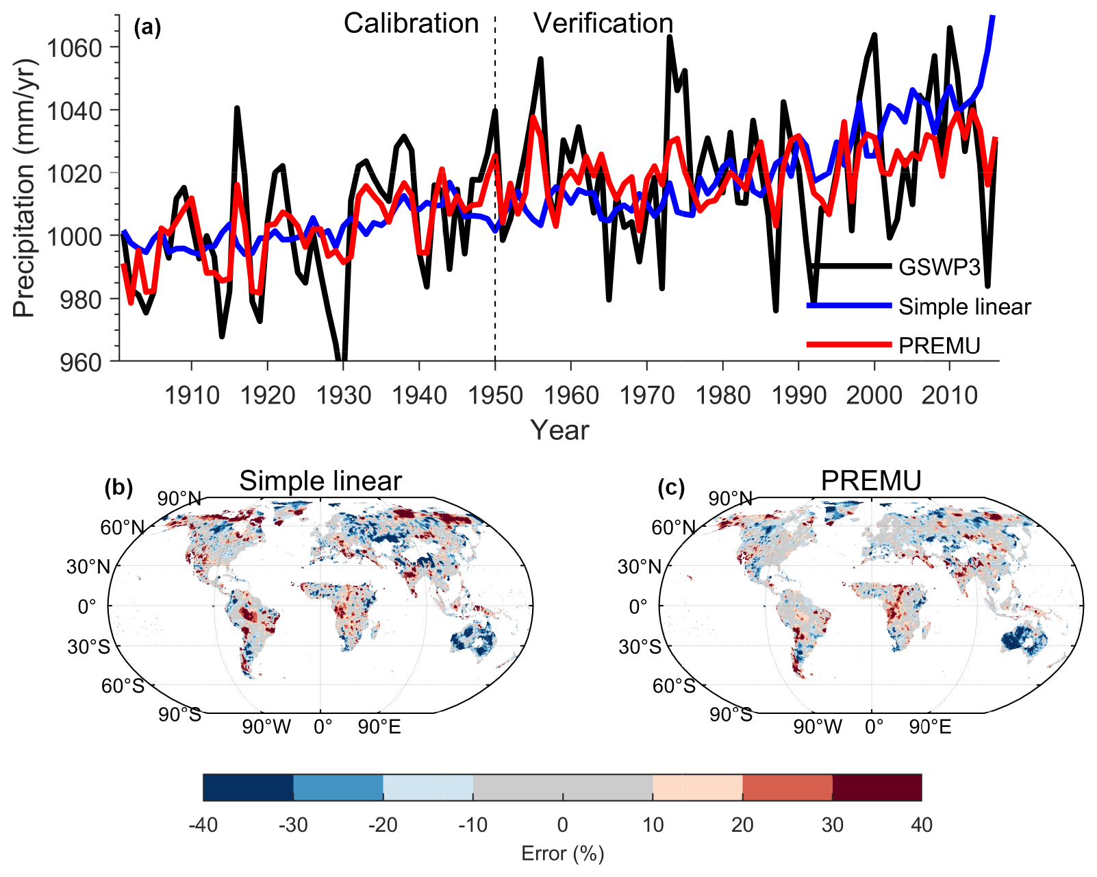
Figure 3 The emulation of historical precipitation. (a) GLAP of the historical observation precipitation (GSWP3) and the predicted precipitation estimated by the simple linear method (simple linear) and by our emulator (PREMU) in 1901–2016. (b) The spatial pattern of error of MAP in 1987–2016 between simple linear and GSWP3. (c) The spatial pattern of error of the MAP in 1987–2016 for our emulator and for GSWP3. The global land average does not include Antarctica because of no emulation for Antarctica, and the arid areas where the MAP from GSWP3 is less than 200 mm yr⁻¹ in 1980–2016 are masked.

4 Results

4.1 Performance of precipitation emulator for historical precipitation

As outlined above, to evaluate the ability of our PREMU to emulate historical precipitation, we first used the precipitation and T_air data from GSWP3 for the period 1901–1951 to calibrate its parameters. We then tested its predictive capability for estimating precipitation data from the period 1951–2016. For the calibration period (1901–1950), our emulator shows a consistent areally averaged global annual precipitation value (1002 and 1002 mm yr⁻¹ for PREMU and GSWP3, respectively) and trend (0.48 and 0.54 mm yr⁻² for PREMU and GSWP3; Table S1). Furthermore, the interannual variations of GLAP derived from PREMU are found to be significantly correlated with those from GSWP3 (R=0.81, p<0.001). For the validation period (1951–2016), PREMU also captured the observed trend (0.22 mm yr⁻² for both PREMU and GSWP3) and interannual variations (R=0.67, p<0.001) of GLAP from GSWP3 (Fig. 3a). In contrast, if we simply used a prediction that linearly relates rainfall changes to global temperature changes and variability, which has similarities to the IMOGEN-based method, we found a much smaller (−0.25 mm yr⁻², −45 %) and larger (+0.47 mm yr⁻², +213 %) trend in GLAP than GSWP3 for the calibration and validation periods, respectively. In addition, the interannual variations of GLAP as estimated by a simple linear regression against global temperature show a weaker correlation with GSWP3 in these two periods (R=0.27, p=0.06 for the calibration period; R=0.15, p=0.21 for the validation period; Fig. 3a; Table S1).

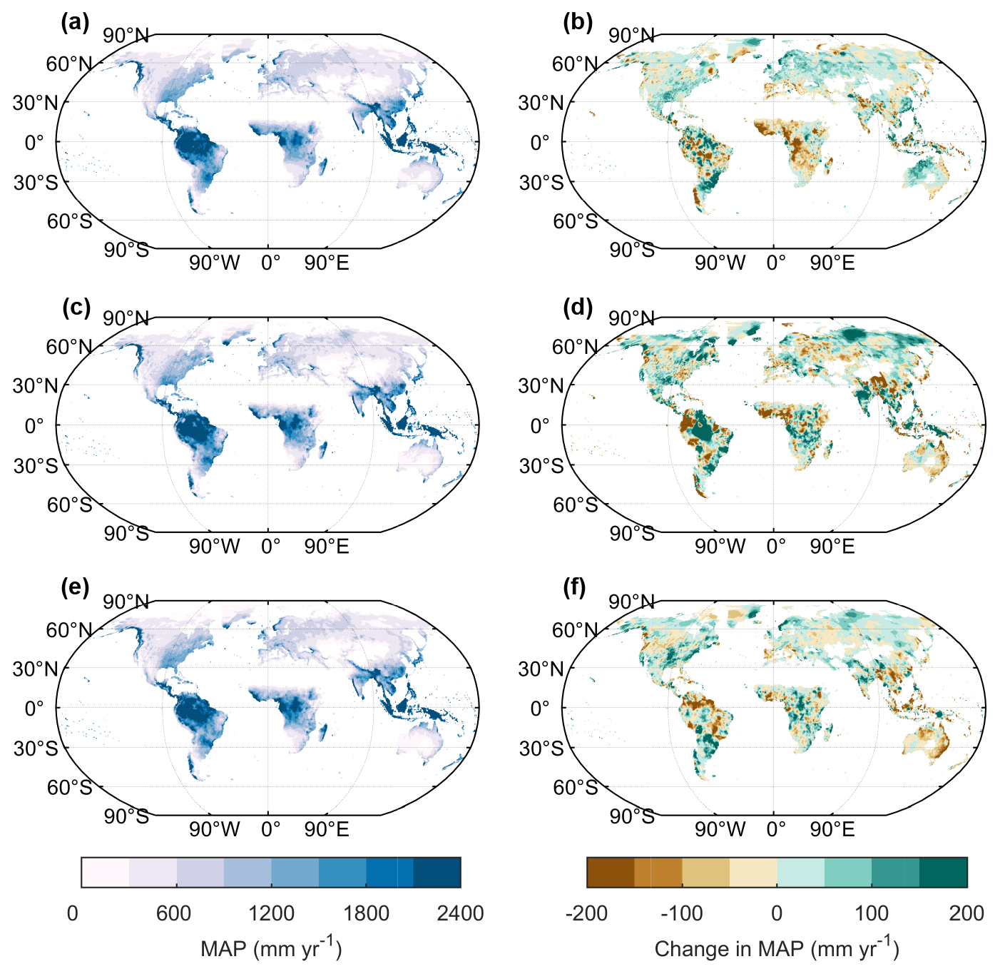
Figure 4 Spatial pattern of MAP and changes in MAP. (a) The MAP in 1987–2016 from GSWP3. (b) The spatial pattern of change in MAP between the period of 1951–1980 and 1987–2016 from GSWP3. (c, d) Same as (a) and (b) but for the emulation from simple linear. (e, f) Same as (a) and (b) but for the emulation from PREMU.

Spatially, PREMU and a simple linear-based method (similar to the algorithms in IMOGEN) can both emulate similarly the spatial pattern of mean annual precipitation (MAP) from the last 3 decades in the validation period (1987–2016), as observed in the GSWP3 data (Fig. 4a, c, e). There are fewer grid cells showing more than 25 % error for MAP from GSWP3 in our emulation (17 %; Table S1) when compared to a simple linear fit (27 %; Fig. 3b and c). The overestimation of MAP with our PREMU method is mainly found in the Tibetan Plateau and central Africa (∼20 %), and the underestimation of MAP is mainly found in northern Siberia, the island of Greenland and northern Australia (−15 % to −30 %; Figs. 3c and S5). To verify the emulator's ability to predict changes in gridded observation precipitation, we calculated the change of MAP in the first and last 3 decades of the validation period (1951–1980 and 1987–2016; Fig. 4b, d, f). For the differences between these two time periods, PREMU shows consistent changes of precipitation in northern Eurasia, North America and central South America and when using GSWP3 data. However, the simple linear method has underestimated the increase or overestimated the decrease of precipitation in these regions (Fig. 4). In some regions of East Asia, Europe, Australia and South America, PREMU underestimates or overestimates the changes in annual precipitation (in the range of 50–200 mm yr⁻¹; Fig. S6), and these values represent little improvement over the simple linear method (Fig. 4). Furthermore, we noted that the changes in MAP from both PREMU and the simple linear method show the opposite to the changes in MAP from GSWP3 in some regions (e.g., Australia and West Africa; Fig. 4b, d, f). This suggests that changes in precipitation in these particular regions may be driven by factors such as aerosols, topography and land use changes rather than temperature, which is further discussed in Sect. 5.

Table 4 Trend of GLAP from ESM average and each ESM and its corresponding emulation by PREMU during the period 2015–2100 under four scenarios. The ESM average represents the multi-model mean precipitation predicted by gridded temperature from nine ESMs. Note that the unit is mm yr⁻².

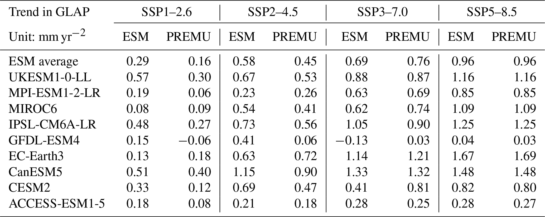
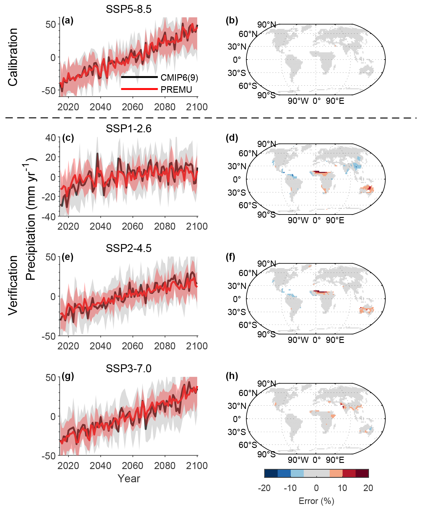
Figure 5 The emulation of future precipitation: (a) multi-model mean GLAP in nine ESMs from CMIP6 (the sixth phase of the Coupled Model Intercomparison Project; CMIP (9)) and the precipitation prediction by our emulator (PREMU) in 2015–2100 under the SSP5–8.5 scenario. The shaded area represents the mean ± SD. (b) The spatial pattern of error in MAP during 2071–2100 for the multi-model mean and our emulator. (c, d) SSP1–2.6; (e, f) SSP2–4.5; (g, h) SSP3–7.0.

4.2 Performance of precipitation emulator in terms of future precipitation from CMIP6 ESMs

A key requirement of PREMU is that it can make projections of precipitation change for different future scenarios of atmospheric GHG concentrations and potentially for novel trajectories of such gases, for which ESMs have not made calculations. To test for this capability, we analyzed its performance at predicting changes under the SSP1–2.6, SSP2–4.5 and SSP3–7.0 scenarios and for those ESM-based simulations that are available. Recall that our PREMU calibration was against ESMs operated for the SSP5–8.5 scenario, capturing inter-ESM differences in projections of T_air and, critically, precipitation. Similar to the emulation for the historical period, PREMU shows a good performance in emulating future precipitation (Fig. 5). For the calibration scenario, the multi-model mean GLAP from PREMU shows a consistent trend (0.96 and 0.96 mm yr⁻² for our emulator and ESMs; Table S2) and interannual variation (R=0.98, p<0.001) with that from ESMs (Fig. 5a). For the three validation scenarios of the different SSPs, PREMU shows a better correlation in interannual variations of GLAP with ESMs than the historical period (R=0.86, p<0.001 for SSP1–2.6; R=0.95, p<0.001 for SSP2–4.5; R=0.95, p<0.001 for SSP3–7.0; Fig. 5c, e, g). Although the trends of global precipitation in our emulation are close to those of ESMs across the three scenarios (Table 4), the error of trends by the PREMU increases from high- to low-emission scenarios (Tables 4 and S3). In addition, the standard deviations of GLAP are underestimated by 2 % in SSP5–8.5 and by 43 % in SSP1–2.6 (Table S2). At the individual ESM level, PREMU can capture well both trends and interannual fluctuations of GLAP under all scenarios for MPI-ESM1-2-LR, MIROC6, EC-Earth3 and CanESM5. For the other five models, there are biases of trends (Table 4) and/or interannual variations of GLAP (Figs. 6 and S7–S9) between our emulation and ESMs. These differences could be partly related to the substantial uncertainties and different features affecting future precipitation projections in ESMs. These factors are discussed in Sect. 5.

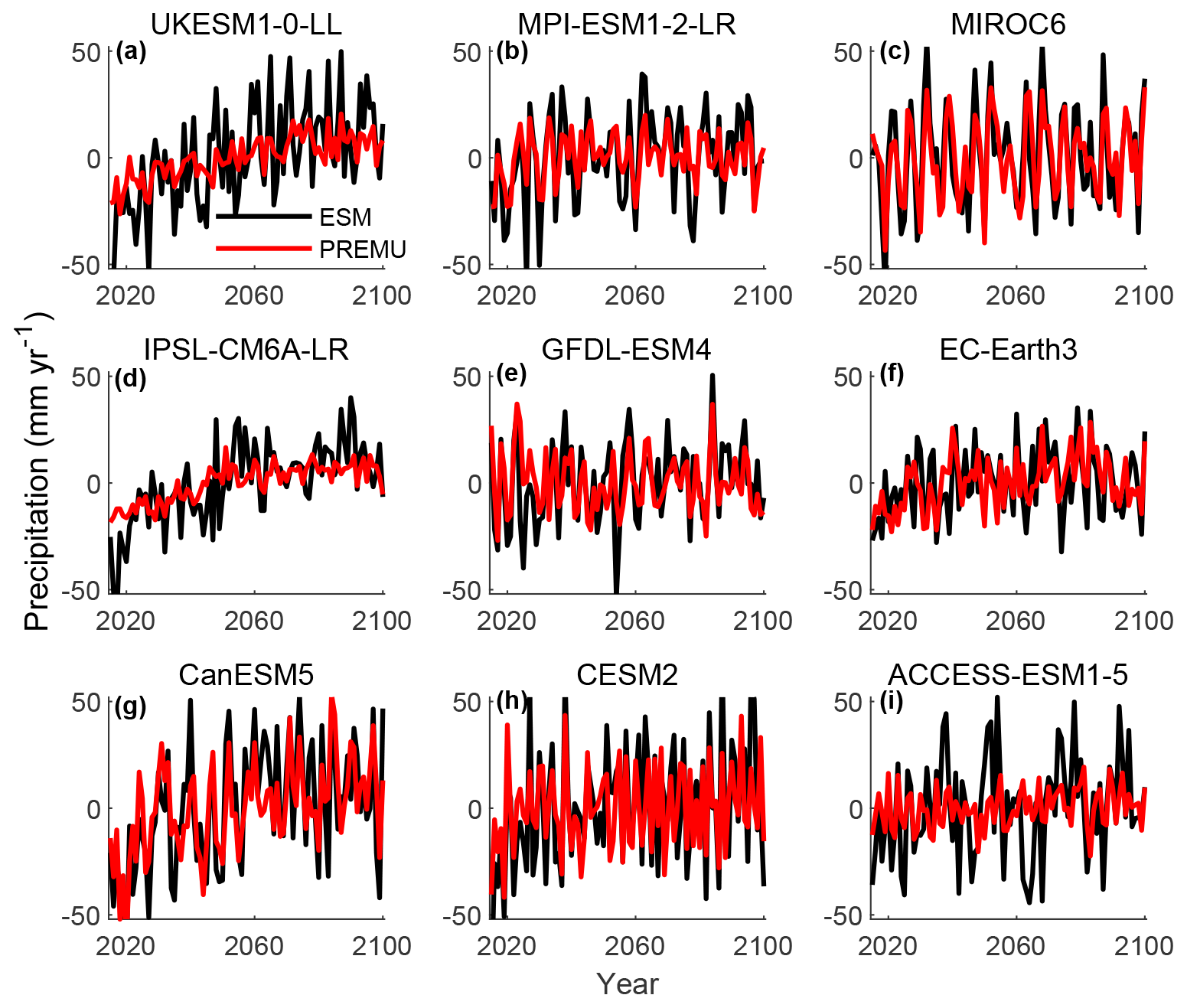
Figure 6 The anomaly of GLAP from each ESM under the SSP1–2.6 scenario: (a) UKESM1-0-LL; (b) MPI-ESM1-2-LR; (c) MIROC6; (d) IPSL-CM6A-LR; (e) GFDL-ESM4; (f) EC-Earth3; (g) CanESM5; (h) CESM2; (i) ACCESS-ESM1-5.

Figure 7 The spatial pattern of MAP in 2071–2100 from (a) multi-model mean of ESMs and (b) the error in MAP from emulation from PREMU. (c, d) SSP1–2.6; (e, f) SSP2–4.5; (g, h) SSP3–7.0.

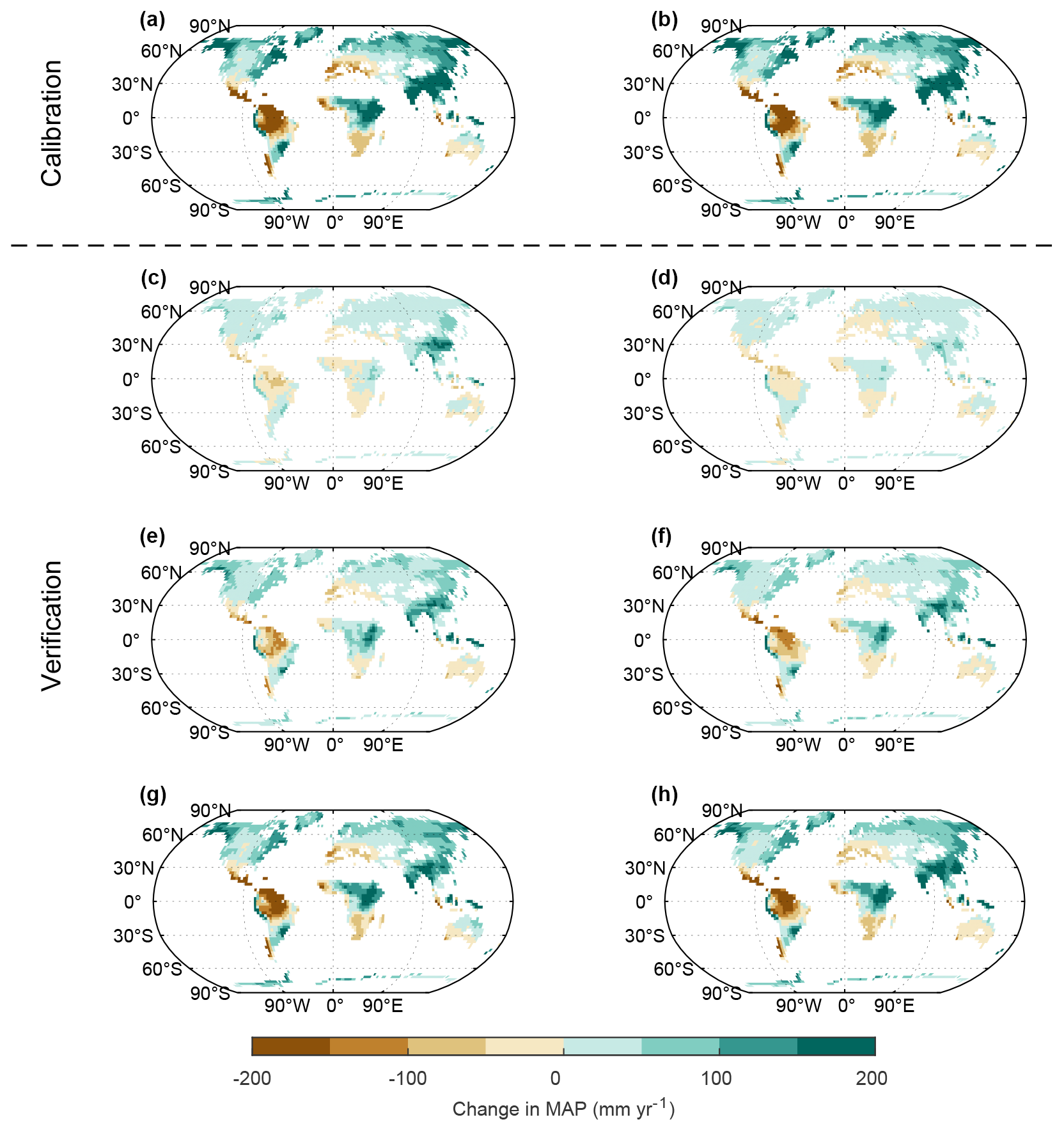
Figure 8 The spatial pattern of change in MAP in 2071–2100 from (a) multi-model mean of ESMs and (b) emulation from PREMU under SSP5–8.5 scenario. (c, d) SSP1–2.6; (e, f) SSP2–4.5; (g, h) SSP3–7.0.

For the spatial pattern (Fig. 5b, d, f, h), PREMU can reproduce the projected pattern of MAP from the multi-model mean of ESMs under the calibration scenario and the three validation scenarios (Fig. 7). Compared to the historical period, the error of multi-model MAP between our emulation and ESMs is relatively smaller (∼10 %; Fig. 7). As for the changes in precipitation during 2015–2100, PREMU shows a consistent canonical pattern of MAP in comparison to the multi-model mean of ESMs (Fig. 8), with a 50–200 mm yr⁻¹ increase of annual precipitation in Eurasia, North America and northeastern Africa but a 50–200 mm yr⁻¹ decrease in the Amazon rainforest from the low- to high-emission scenarios. However, similar to the simulation for GLAP, the error in the spatial pattern of MAP and changes in MAP between our emulation and ESMs increases from high- to low-emission scenarios (Figs. 5 and 8). Furthermore, compared to the historical period, PREMU can capture the changes in MAP in West Africa well under all four scenarios, but it also emulated the opposite changes of MAP in Australia under SSP3–7.0, which is discussed in Sect. 5. When considering performance at the individual ESM level, PREMU can reproduce the spatial pattern of MAP well. In general, the proportions of grid cells with an error more than 10 % are small (8 % [6 %–14 %] for SSP1–2.6; 5 % [3 %–8 %] for SSP2–4.5; 5 % [3 %–9 %] for SSP3–7.0; 0 % [0 %–0 %] for SSP5–8.5; mean [min–max]; Figs. 9 and S10–S12). However, as for the changes in MAP, we found a relatively poor performance in emulating the changes in some ESMs, especially in SSP1–2.6 (Figs. 10 and S13–S15). While the spatial pattern of changes in MAP is quite different across ESMs, even under the same SSP, the errors by PREMU are much smaller than the inter-ESM differences (Figs. 10 and S13–S15).

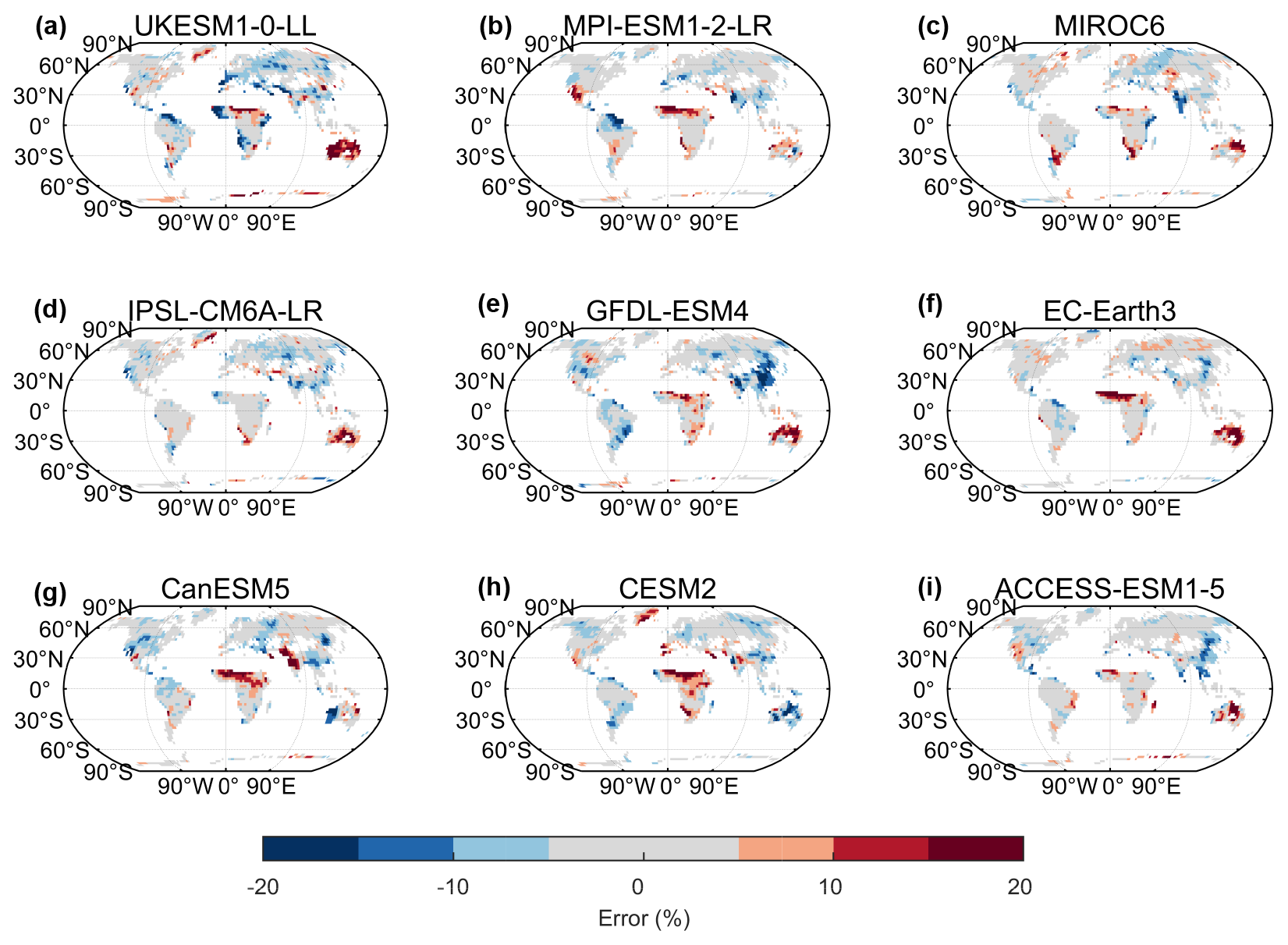
Figure 9 The spatial pattern of the error of the MAP in 2071–2100 between each ESM and emulation from PREMU under the SSP1–2.6 scenario: (a) UKESM1-0-LL; (b) MPI-ESM1-2-LR; (c) MIROC6; (d) IPSL-CM6A-LR; (e) GFDL-ESM4; (f) EC-Earth3; (g) CanESM5; (h) CESM2; (i) ACCESS-ESM1-5.

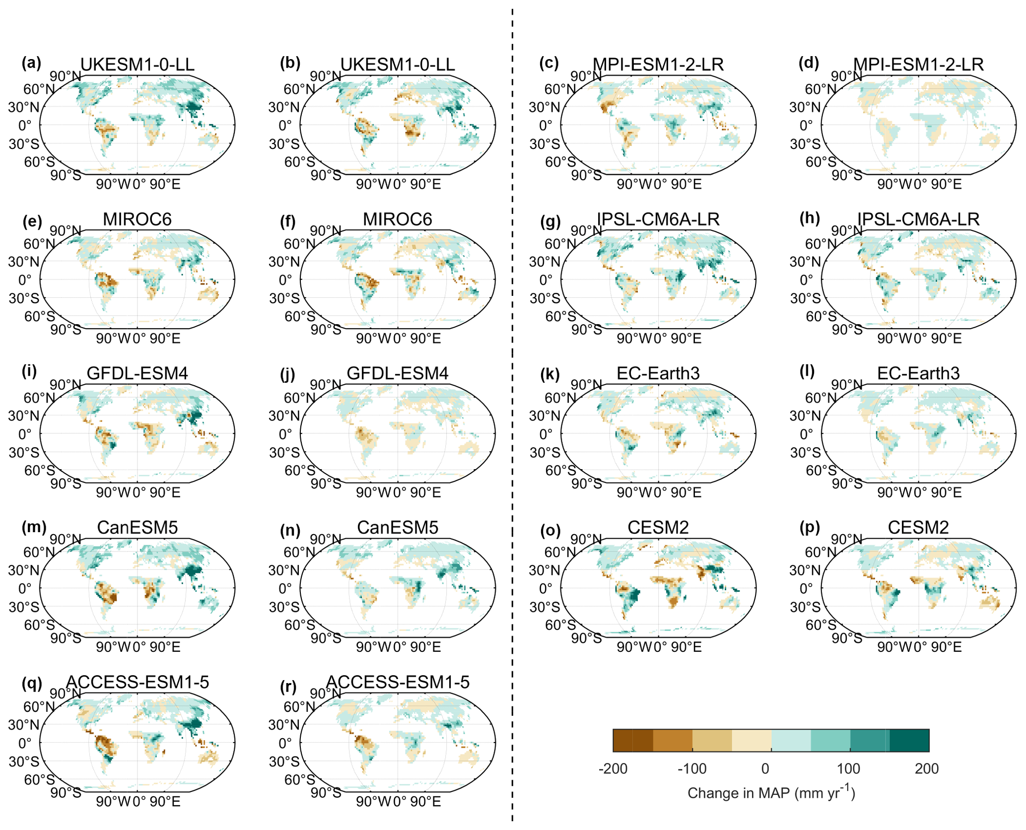
Figure 10 The spatial pattern of change in MAP between the period of 2015–2044 and 2071–2100 from (a) UKESM1-0-LL and (b) emulation from PREMU under SSP1–2.6 scenario. (c, d) MPI-ESM1-2-LR; (e, f) MIROC6; (g, h) IPSL-CM6A-LR; (i, j) GFDL-ESM4; (k, l) EC-Earth3; (m, n) CanESM5; (o, p) CESM2; (q, r) ACCESS-ESM1-5.

Figure 11 (a) The seasonal cycle of 30–90^∘ N latitude land average precipitation in 1987–2016 from GSWP3, simple linear method and PREMU; (b) 0–30^∘ N; (c) 30^∘ S–0^∘; (d) 90–30^∘ S.

4.3 Seasonal performance of precipitation emulator

As a monthly emulator, the performance of PREMU in describing the seasonal cycle of precipitation requires evaluation. For the historical observations, PREMU can capture the seasonal cycle of GLAP in each latitude band (Fig. 11). There are some spatial differences, with little error in boreal regions but with 18–22 mm per month error in the tropics (Fig. S16). We found fewer grid cells showing more than 20 mm per month error of seasonal precipitation from GSWP3 in our emulation (18 %–24 %) compared to using a simple linear fit (24 %–31 %; Fig. S16). As for the future precipitation, PREMU shows a good performance in emulating the monthly land average precipitation in each latitude band under all scenarios (Fig. S17). However, PREMU tends to overestimate the JJA (June, July, August) and SON (September, October, November) precipitation in South Asia and the Amazon and underestimates the SON and DJF (December, January, February) precipitation in West Africa under SSP1–2.6, while the error in the spatial pattern of seasonal precipitation decreases from low- to high-emission scenarios (Fig. S18).

5 Discussion

To our knowledge, this study provides a novel approach to linking local precipitation changes to geographical features (i.e., spatial modes) of gridded temperature in a single emulator chain, which can be further incorporated into existing LCMs. Despite relying on a series of simple assumptions, PREMU can successfully capture the changes in precipitation simulated by ESMs and under a broad range of different emission scenarios. Comparing with the precipitation predicted by a simple linear regression between local rainfall alteration and the level of global warming (e.g., as used in other LCMs such as IMOGEN), the rainfall in PREMU shows more consistent trends and interannual variations of GLAP and in the spatial pattern of MAP. These improvements are noted in the comparison against the historical precipitation recorded in the GSWP3 dataset, as well as when emulating the future precipitation predicted by ESMs (Figs. 3–6). For a user-prescribed emission scenario or for a time-evolving global temperature trajectory designed to constrain warming to a level such as 2 ^∘C (Huntingford et al., 2017), PREMU can accurately and quickly emulate the related gridded precipitation changes. Our method can utilize the existing spatial features of gridded temperature from either ESMs or LCMs to support studies related to future changes in precipitation. In particular, coupling our precipitation emulator with other LCMs provides the input climate forcing for land surface models to help disentangle hydrological and ecological responses globally to future climate change (Zelazowski et al., 2018; Li et al., 2022; Korell et al., 2021).

5.1 Possible cause for the emulation errors of PREMU

We noted that the performance of PREMU in predicting future precipitation from ESMs is much better than that when emulating historical GSWP3 precipitation. This is because PREMU is only based on the 10 modes of global gridded temperature, and the effects of aerosols and topography on precipitation are not well represented in our emulator (Austin and Dirks, 2005; Medvigy and Beaulieu, 2012). For instance, Fig. 3 shows that emulated precipitation has large errors in mountainous regions, where orographic precipitation could be dominant. The effect of raised aerosols in the 20th century has been shown to have a role almost as large as greenhouse gas warming effects on features of regional precipitation (e.g., in India; Bollasina et al., 2011). Thus, adding the effects of topography and aerosols on precipitation into the PREMU could further improve the ability to predict precipitation. Considering that the changes in MAP in West Africa from PREMU are opposite to the changes in MAP from GSWP3 (Fig. 4), PREMU can emulate the changes in MAP in West Africa from ESMs well. An alternative argument is that the good performance by PREMU in predicting precipitation from ESMs may suggest that climate models underrepresent the effects of topography and aerosols (Samset et al., 2016; Yang et al., 2021).

Overall, the performance of predicting precipitation from ESMs by our emulator is good, although not for all models and under all scenarios. Both trends and interannual variability of GLAP are well captured under all scenarios for MPI-ESM1-2-LR, MIROC6, EC-Earth3 and CanESM5, but PREMU performs less well when predicting GLAP in the other five ESMs (Figs. 6 and S7–S9). This may be because different ESMs use alternative atmospheric circulation models and precipitation schemes (e.g., CAM6.3 in CESM2 and AM4 in GFDL-ESM4), which contain different physical processes or parameterizations in their simulation of precipitation (Danabasoglu et al., 2020; Horowitz et al., 2020; Hourdin et al., 2020). Notable is that PREMU underestimates 30 % (6 %–60 %) of interannual variations of precipitation in all ESMs and when considering across all four GHG concentration scenarios. This is a common “feature” of linear regression models, as they favor bias reduction over variance under the bias–variance trade-off (Geman et al., 1992). In addition, we also suggest that this may be because of missing some modes (out of the 10 modes we used) for interannual variations, an underrepresentation of the effect of key climate modes such as ENSO in our emulator or a non-linear response of precipitation to climate modes. It is also worth noting that the trend of GLAP in CESM2 and GFDL-ESM4 under SSP3–7.0 is lower than that under SSP2–4.5. We speculate that this may be caused by the most drastic land use changes associated with that former SSP scenario, resulting in a slower increase in precipitation under SSP3–7.0 (Riahi et al., 2017). Our emulator predicts precipitation through the temperature gradients and so cannot capture the impact of land use changes on precipitation via altered land–atmospheric feedbacks that impact the hydrological cycle (Table 4).

5.2 Evaluating the assumptions in methods

Our emulator is based on the assumption that spatial temperature modes can describe precipitation well. Hence, we assumed implicitly that the coefficient matrixes in PCA for global gridded temperature (i.e., the weights of each grid cell for each principal component) are stable, i.e., invariant, with climate change. To test this assumption, we compared the coefficient matrixes of temperature derived for the SSP5–8.5 scenario with those from the SSP1–2.6 scenario for the modeled period 2015–2100 (Figs. S16 and S17). For the future scenarios, we found that most coefficients of PCA, in both January and July, are similar between the SSP5–8.5 scenario and SSP1–2.6 scenario. Though with a different order of PCA coefficients (Figs. S19–S20), this finding suggests that the main features of global temperature are constant across different scenarios. We noted that, in some instances, the signs of coefficients are opposite for some principal components between different scenarios, but this also corresponds to regression coefficients with opposite signs, which combined give the same predictions. Depending on the circumstances, we noted that it may not be necessary to use all top 10 PCs. For instance, if researchers only require the decadal average or any increasing trend in precipitation, PREMU calibrated by the top 1 PC of T_air under SSP5–8.5 may be sufficient to capture these characteristics of GLAP from ESMs and under all four scenarios (Fig. S21). If the researchers only require the decadal average or the trend of precipitation, PREMU calibrated by the top 1 PC of T_air under SSP5–8.5 can also capture the trends of GLAP from ESMs under all four scenarios (Fig. S21). Furthermore, we have assumed that the coefficients of PCA are linked with the ocean–atmosphere oscillations, but the detailed physical explanations of the coefficient matrix need further study in the future.

We have confirmed that our ability to reproduce the historical and future trends, as well as interannual variabilities in precipitation, is better than with other methods that more simply regress local changes against global temperature variation (e.g., IMOGEN and OSCAR; Zelazowski et al., 2018; Gasser et al., 2017). However, the remaining biases in emulating the other three SSPs with the emulator constructed (i.e., fitted) under SSP5–8.5 imply that the sensitivity of gridded precipitation to temperature modes may have a slight dependence on SSP. There are some studies that predict an increased variability in precipitation under a warmer world (Zhang et al., 2021; Song et al., 2018), but where such additional variability is not present in the spatial temperature modes of variations. Therefore, it could be unwise to use the emulator constructed using the temperature and precipitation during the historical period or under the low-emission scenarios to project future precipitation change under a high-emission scenario. Constructing the emulator separately for low- or high-emission scenarios could help reduce uncertainties in emulating future precipitation. When coupling PREMU with other LCMs to emulate the gridded precipitation under a new prescribed emission scenario, we suggest calibrating PREMU against the SSP whose future temperature most closely resembles the temperature in LCMs under that new scenario.

5.3 Other versions of PREMU

5.3.1 PREMU constructed by different temperature lag periods

We tested the effect of different lags of gridded temperature on changes in precipitation. Previous studies noted that “memory effects” may cause precipitation to be affected more by the climate modes in the previous months (An et al., 2020). Throughout this study, we used the 3-month average temperature (month of interest plus the previous two months) to capture potential lagging effects. However, to quantify the uncertainty based on duration of the lag effect, we also tested 1-month temperature and 6-month average temperature to construct the emulator, respectively (“emulator-1mon” and “emulator-6mon”). For the historical period, we found that the emulator-1mon was unable to capture the increase of GLAP after 1950. Predicting the GLAP from emulator-6mon shows a good fitting of the trends and interannual variations of GLAP in GSWP3, similar to that from the emulator based on 3-month average temperature but with a lower correlation coefficient (R=0.77, p<0.001 for 3 months; R=0.73, p<0.001 for 6 months; Fig. S22). For future precipitation from ESMs, all three emulators with different temperature lag periods (1 month, 3 months, 6 months) can capture well the changes in GLAP and gridded precipitation under different scenarios in the future (Figs. S23 and S24). This may be due to underrepresentation of topography and aerosol effects in ESMs, which are potential sources of variations in precipitation and could be important for influencing the lag differences. Hence, we deduced that the method is highly robust (i.e., invariant) in terms of lag length when emulating the future precipitation (Figs. 5 and S23–S24).

5.3.2 PREMU constructed by T_air over land

We constructed our emulator using thermal modes of variation based on the temperature from over both land and ocean grid cells. As a sensitivity study, we also evaluated the performance of the emulator constructed using only T_air over land (“emulator-land”) to test its capability at predicting future precipitation. We found that the emulator-land can also reproduce consistent trends and interannual variations of GLAP and changes in gridded precipitation found with ESMs (Figs. S25 and S26), while the correlation in terms of interannual variations of GLAP with ESMs is relatively lower than PREMU (R=0.71 for SSP1–2.6; R=0.88 for SSP2–4.5; R=0.91 for SSP3–7.0; R=0.96 for SSP5–8.5). Considering that the change of air temperature over ocean could contain additional information that relates to local climate variability (Trenberth and Shea, 2005), we suggest retaining our inclusion of all land and ocean grid cells in PREMU calibration.

5.4 Potential further developments of PREMU

Our emulator has focused on total precipitation at each location. Future analyses could include testing its performance for individual features or subsets of precipitation patterns, such as convective precipitation, large-scale precipitation and topographic precipitation. We also suggest possibly extending our emulator drivers beyond the modes of variability of air temperature only. For example, considering that the interannual variations of precipitation are mainly caused by large-scale precipitation dominated by ENSO (Cai et al., 2001; van Oldenborgh and Burgers, 2005; Gupta and Jain, 2021; Zhou et al., 2020), we could consider additionally entraining sea surface temperature as a forcing variable. Similarly, for convective precipitation, local temperature and energy for uplift could be used for prediction (Berg et al., 2013). Furthermore, PREMU may not have good capability in emulating the seasonal cycle of gridded precipitation. We suggest that a future improvement, which will allow projections at sub-yearly timescales, might be to add a residual variability module similar to that in the MESMER-M model via lag-1 autocorrelations or local spatially correlated processes (Nath et al., 2022).

6 Conclusions

In this study, we proposed an algorithm to construct a precipitation emulator, which could estimate gridded precipitation and its changes in a convenient and computationally effective way. We exploit strong discovered linkages between rainfall patterns and natural spatial modes of variability in near-surface temperature. To the best of our knowledge, this is a pioneer emulator that can be directly coupled within existing LCMs, especially noting that LCMs may perform well for other variables but are currently weaker at estimating features of rainfall. This new combination will better predict global and gridded precipitation under different emission scenarios. With illustrative examples, we demonstrated the good performance of our emulator in predicting the absolute value and interannual variations in historical precipitation from GSWP3 and also in predicting future precipitation under four scenarios from ESMs. In addition, we also verified the reliability of our results despite the potential uncertainties in the method (e.g., the assumptions of the stability of the coefficient matrix in PCA and the sensitivity of gridded precipitation to temperature modes). The accurate projection of future precipitation can help analyze not only expected direct climate change under different emission scenarios but also the responses of the hydrological cycle and ecological processes to such future changes. ESMs remain hugely computationally demanding and can be only operated for a limited number of century-scale projections. Hence, robust emulators of full-complexity Earth system models remain an important tool, extrapolating ESM projections to alternative future emissions or GHG concentration scenarios that require investigation and understanding.

Appendix A: Table of abbreviations

CMIP6	The sixth phase of the Coupled Model Intercomparison Project
EBM	Energy balance model
ESM	Earth system model
GLAP	Global land average precipitation
GSWP3	Global Soil Wetness Project Phase 3
IMOGEN	Integrated Model Of Global Effects of climatic aNomalies (Zelazowski et al., 2018)
LCM	Lower-complexity models
MAP	Mean annual precipitation
MESMER	Modular Earth System Model Emulator with spatially Resolved output (Beusch et al., 2022)
OSCAR	A compact Earth system model (see Gasser et al., 2017)
PCA	Principal-component analysis
PREMU	A computationally efficient precipitation emulator (this study)
SSP	Shared socioeconomic pathway
Tair	Surface air temperature