A nonhydrostatic oceanic regional model, ORCTM v1, for internal solitary wave simulation

The Oceanic Regional Circulation and Tide Model (ORCTM), including a nonhydrostatic dynamics module which can numerically reproduce internal solitary wave (ISW) dynamics, is presented in this paper. The performance of a baroclinic tidal simulation is also examined in regional modeling with open boundary conditions.

The model control equations are characterized by three-dimensional and fully nonlinear forms considering incompressible Boussinesq fluid in Z coordinates. The pressure field is decomposed into the surface, hydrostatic, and nonhydrostatic components on the orthogonal curvilinear Arakawa-C grid. The nonhydrostatic pressure determined by the intermediate velocity divergence field is obtained via solving a three-dimensional Poisson equation based on a pressure correction method. Model validation experiments for ISW simulations with the topographic change in the two-layer and continuously stratified ocean demonstrate that ORCTM has a considerable capacity for reproducing the life cycle of internal solitary wave evolution and tide–topography interactions.

1 Introduction

Internal wave (also called internal gravity waves) activities have been observed frequently across the stratified ocean and play a significant role in the multiscale energy cascade (Mtfller, 1976). Observations reveal that internal waves, especially high-frequency internal solitary waves, could contain significant potential energy with strong vertical shear, mixing, and wave breaking, leading to a dramatic change in the currents and density structures (Ramp et al., 2004; Vlasenko et al., 2010; Huang et al., 2016), violent overturning bringing sediment and nutrients from the seafloor to the surface (Wang et al., 2007), and even damage to some underwater vehicles (Duda et al., 2006) and deep-water drilling projects (Osborne et al., 1978). Basically, astronomical tides passing abrupt topography can cause the generation of baroclinic tides (also called internal tides, hereafter ITs) with multi-modal structures then capable of propagation, disintegration, and dissipation in the ocean (Vlasenko et al., 2005, 2010). The low mode of baroclinic tides can travel thousands of kilometers with long horizontal wavelengths of tens of kilometers (Baines, 1982). Furthermore, the inclusion of nonlinear and nonhydrostatic effects permits the evolution of nonlinear internal waves (hereafter NIWs) and even internal solitary waves (hereafter ISWs) derived from the steepening of low-mode internal tides as the consequence of the ever-changing terrain and background stratification (Gerkema and Zimmerman, 1995; Legg and Adroft, 2003).

Numerical ocean models are one of the most effective tools to study internal waves compared to theoretical methods, in situ observations, and laboratory investigations. Ocean models with the hydrostatic balance approximation have been used to explore the regional circulation and tide dynamics across the stratified ocean. The hydrostatic balance manages to take the large scales to mesoscales into consideration due to the fairly high accuracy (Marshall et al., 1997b; Chen et al., 2003; Shchepetkin and McWilliams, 2005; Ko et al., 2008). However, In the hydrostatic balance scheme, omitting some essential terms in the vertical momentum equation results in the inapplicability of nonhydrostatic dynamics (Lai et al., 2010). For example, the subsequent steepening of the internal tides and the later high-frequency nonlinear ISW formation cannot be depicted by a hydrostatic modeling whereby only internal jumps are formed but no soliton appears (Li, 2014) because the strong vertical current with its order of magnitude equals the horizontal one via the scale analysis method (Marshall et al., 1997a). In other words, the three-dimensional Navier–Stokers equations should be considered thoroughly. It is indispensable for simulating the nonlinear and large-amplitude ISWs to develop a nonhydrostatic ocean model in consideration of nonhydrostatic dynamics.

A robust ocean model with nonhydrostatic dynamics realizations should satisfy at least two requirements synchronously: (1) high enough accuracy of mesoscale to large-scale simulations must be guaranteed, such as large-scale wind-induced circulation and mesoscale eddies reconstructed and mainly influenced by the hydrostatic balance. (2) Meanwhile, they should be concerned with small scales to mesoscales with higher spatial and temporal resolution that are resolved finely under the nonhydrostatic balance; for instance, there is a simulation able to describe the cradle-to-grave process for tide–topography interactions, the dispersive effects and nonlinear steepening of baroclinic tides, and the breaking and dissipation of strong nonlinear ISWs. The nonhydrostatic simulation can apply to the small to large scales across the stratified ocean simultaneously, which is identified as one of the main directions for research and development of the nonhydrostatic ocean model. In reality, there have been some nonhydrostatic ocean models or ones considering nonhydrostatic dynamics coming out in the past decades, such as MITgcm (Marshall et al., 1997a, b, 1998), SUNTANS (Fringer et al., 2006), and ROMS (Kanarska et al., 2007). All of the above have been used to realize a series of two- or three-dimensional nonhydrostatic numerical studies, including the instability of small-scale flows in laboratory experiments (Lai et al., 2010; Li et al., 2022), internal solitary waves in the continental shelves (Vlasenko et al., 2010; Zeng et al., 2019), and the hydraulic lee wave around the seamount (Kanarska et al., 2007; Liu et al., 2016). Nevertheless, the primary reason why there is still no widespread use for the nonhydrostatic ocean model is that the nonhydrostatic solution to an extensive sparse linear equation is too demanding to solve directly for the 3-D oceanic environment. That usually demands large iteration times, fast convergence speed, and large PC storage. For this reason, Ai and Ding (2016) employed a novel model grid arrangement to render the sparse linear equation discretized form simpler to solve where the bottom-fitted coordinate ensures the homogeneous boundary condition. Moreover, numerical errors can be avoided via the immersed boundary method to treat uneven bottoms in the calculation of the baroclinic pressure force (Ai et al., 2021). Generally, whether the boundary conditions are matched with the whole nonhydrostatic algorithm can shape the performance of complex nonhydrostatic dynamics in the regional ocean model. In addition, the different kinds of sub-grid parameterization schemes have a profound impact on the model performance with a necessity for appropriate ones to be assessed, and most of these model codes are seldom shared or open-source. Supposing we develop a nonhydrostatic ocean model based on an original hydrostatic framework model. In that case, the nonhydrostatic dynamics module should involve a complete vertical momentum equation. Some terms associated with the vertical velocity are required to be complemented simultaneously in the other equation. Also, based on the idea of the fractional step method (Press et al., 1988; Armfield and Street, 2002), the total pressure is to be decomposed into hydrostatic and nonhydrostatic components (Marshall et al., 1997a; Lai et al., 2010). The former corresponds to the result of hydrostatic balance, and the divergence for intermediate velocity limits the latter to correct the local velocity fields, called the “pressure correction” method (Stansby and Zhou, 1998; Fringer et al., 2006; Kanarska et al., 2007; Lai et al., 2010). With these methods, the nonhydrostatic dynamics simulation can be economically fulfilled comparatively in harmony with the original physical framework as an extension of the hydrostatic ocean model.

In this context, we have implemented the nonhydrostatic dynamic algorithm into the Oceanic Regional Circulation and Tide Model (hereafter ORCTM) and demonstrated its capability and performance of reproducing the life cycle of nonlinear internal solitary waves in distinct hydrodynamic environments. The rest of the paper is organized as follows. In Sect. 2, the basic framework of ORCTM including control equations, open boundary conditions, and nonhydrostatic algorithms is described. In Sect. 3, a series of numerical validation experiment results is presented, aiming at the simulation of the overall processes of internal solitary waves. In the last section, we have some further discussions and come to conclusions.

2 Model development

The Max Planck Institute Ocean Model (MPI-OM) is a global ocean circulation and tide model based on the ocean primitive equations discretized on the orthogonal curvilinear Arakawa-C grid with hydrostatic balance approximation (Marsland et al., 2003; Chen et al., 2005). Rooted from MPI-OM, in this paper, an oceanic regional circulation and tide model (ORCTM) has been developed to realize the simulation for nonhydrostatic internal solitary wave modeling, which will be referred to hereafter as ORCTM version 1.0. The z-level grid applied has the partial filled cell capability to adjust the distance of the vertical grid on the seabed for fitting into the realistic terrain, and the tidal forcing flow can be implemented via a relaxation scheme at the open boundary with an area of sponge layers. It is under the laws of the Boussinesq, rotating, and fully nonlinear Navier–Stokes fluid that ORCTM can be used to reproduce and explore the nonhydrostatic dynamics such as large-amplitude ISWs, nonlinear tidal internal waves, and downwelling and upwelling processes of real oceans.

2.1 Control equations

The three-dimensional ocean primitive control equations involve the momentum, continuity, potential temperature, salinity, and density equations given as follows.

$$\begin{array}{}\text{(1)}& {\displaystyle }\begin{array}{rl}{\displaystyle \frac{\partial u}{\partial t}}& +u{\displaystyle \frac{\partial u}{\partial x}}+v{\displaystyle \frac{\partial u}{\partial y}}+w{\displaystyle \frac{\partial u}{\partial z}}-fv+\stackrel{\mathrm{̃}}{f}w=-{\displaystyle \frac{\mathrm{1}}{{\mathit{\rho }}_c}}{\displaystyle \frac{\partial P}{\partial x}}\\ & -g{\displaystyle \frac{\partial \mathit{\varsigma }}{\partial x}}+F_{\mathrm{V}x}+F_{\mathrm{H}x}+F_x\end{array}\text{(2)}& {\displaystyle }\begin{array}{rl}{\displaystyle \frac{\partial v}{\partial t}}& +u{\displaystyle \frac{\partial v}{\partial x}}+v{\displaystyle \frac{\partial v}{\partial y}}+w{\displaystyle \frac{\partial v}{\partial z}}+fu=-{\displaystyle \frac{\mathrm{1}}{{\mathit{\rho }}_c}}{\displaystyle \frac{\partial P}{\partial y}}-g{\displaystyle \frac{\partial \mathit{\varsigma }}{\partial y}}\\ & +F_{\mathrm{V}y}+F_{\mathrm{H}y}+F_y\end{array}\text{(3)}& {\displaystyle }\begin{array}{rl}{\displaystyle \frac{\partial w}{\partial t}}& +u{\displaystyle \frac{\partial w}{\partial x}}+v{\displaystyle \frac{\partial w}{\partial y}}+w{\displaystyle \frac{\partial w}{\partial z}}-\stackrel{\mathrm{̃}}{f}u=-{\displaystyle \frac{\mathrm{1}}{{\mathit{\rho }}_c}}{\displaystyle \frac{\partial P}{\partial z}}-{\displaystyle \frac{\mathit{\rho }}{{\mathit{\rho }}_c}}g\\ & +F_{\mathrm{V}z}+F_{\mathrm{H}z}+F_z\end{array}\text{(4)}& {\displaystyle \frac{\partial u}{\partial x}}+{\displaystyle \frac{\partial v}{\partial y}}+{\displaystyle \frac{\partial w}{\partial z}}=\mathrm{0}\text{(5)}& {\displaystyle }{\displaystyle \frac{\partial \mathit{\theta }}{\partial t}}+u{\displaystyle \frac{\partial \mathit{\theta }}{\partial x}}+v{\displaystyle \frac{\partial \mathit{\theta }}{\partial y}}+w{\displaystyle \frac{\partial \mathit{\theta }}{\partial z}}=F_{\mathrm{V}\mathit{\theta }}+F_{H\mathit{\theta }}+Q_{\mathit{\theta }}\text{(6)}& {\displaystyle }{\displaystyle \frac{\partial S}{\partial t}}+u{\displaystyle \frac{\partial S}{\partial x}}+v{\displaystyle \frac{\partial S}{\partial y}}+w{\displaystyle \frac{\partial S}{\partial z}}=F_{\mathrm{V}S}+F_{\mathrm{H}S}+Q_s\text{(7)}& {\displaystyle }\mathit{\rho }=\mathit{\rho }\left(\mathit{\theta },S,P\right)\end{array}$$

In the local Cartesian framework of reference on the rotating Earth for a geophysical flow, t is the time; $\partial /\partial t$ is the time partial derivative; x,y, and z axes are directed eastward, northward, and upward, respectively; the horizontal velocity vector is ${\mathit{u}}_h=\left(u,v\right)$; and w is the vertical velocity. With the linearized kinematic boundary condition and the freshwater forcing term Q_ς from the evaporation and precipitation (Marsland et al., 2003), the free surface elevation equation can be proposed as follows.

$$\begin{array}{}\text{(8)}& {\displaystyle \frac{\partial \mathit{\varsigma }}{\partial t}}=-{\mathrm{\nabla }}_{\mathrm{h}}\cdot {\int }_{-H}^{\mathit{\varsigma }}{\mathit{u}}_{\mathrm{H}}\mathrm{d}z+Q_{\mathit{\varsigma }}\end{array}$$

ς is the change in the free surface elevation; P, θ, and S are pressure, potential temperature, and salinity; and ρ_c is the reference density of seawater. The first and second Coriolis parameters are f=2Ωsin φ and $\stackrel{\mathrm{̃}}{f}=\mathrm{2}\mathrm{\Omega }\cos \mathit{\phi }$, where Ω is the rotational angular speed and φ is the geographic latitude. ∇_H is the horizontal divergence operator; Q_θ and Q_s are source or sink terms about potential temperature and salinity. The equation of seawater state is the polynomial form for the density ρ advocated by the Joint Panel on Oceanographic Tables and Standards (Fofonoff and Millard, 1983). The additional forcing term vector $\mathit{F}=\left(F_x,F_y,F_z\right)$ can consider tidal potential forcing. The horizontal eddy viscosity vector is ${\mathit{F}}_{\mathrm{H}}=\left(F_{\mathrm{H}x},F_{\mathrm{H}y},F_{\mathrm{H}z}\right)$ described with the scale-dependent biharmonic formulation (Wolff et al., 1997; Marsland et al., 2003), and the horizontal diffusivity terms of temperature and salinity are F_Hθ and F_HS, supporting the harmonic forms. In addition, the vertical eddy viscosity vector is ${\mathbf{F}}_{\mathrm{V}}=\left(F_{\mathrm{V}x},F_{\mathrm{V}y},F_{\mathrm{Vz}}\right)$ and eddy diffusivity terms are F_Vθ and F_VS. Here, the vertical eddy turbulent frictions are specified to depend on the Richardson number Ri via the modified PP81 parameterization scheme (Pacanowski and Philander, 1981). The viscous terms above are expressed as follows.

$$\begin{array}{}\text{(9)}& {\displaystyle }{\mathit{F}}_{\mathrm{H}}=-{\mathrm{\nabla }}_{\mathrm{h}}\cdot \left(B_{\mathrm{H}}{\mathrm{\nabla }}_{\mathrm{h}}\mathrm{\Delta }\mathit{u}\right),{\mathit{F}}_{\mathrm{V}}={\displaystyle \frac{\partial }{\partial z}}\left(A_{\mathrm{V}}{\displaystyle \frac{\partial \mathit{u}}{\partial z}}\right)\text{(10)}& {\displaystyle }{F}_{\mathit{\chi }\mathrm{H}}=D_{\mathrm{H}}\mathrm{\Delta }\mathit{\gamma },F_{\mathit{\chi }V}={\displaystyle \frac{\partial }{\partial z}}\left(D_{\mathrm{V}}{\displaystyle \frac{\partial \mathit{\chi }}{\partial z}}\right),\mathit{\chi }=\mathit{\theta },S\text{(11)}& {\displaystyle }\begin{array}{rl}{A}_{\mathrm{V}}^{n+\mathrm{1}}& =\left(\mathrm{1}-\mathit{\lambda }\right)A_{\mathrm{V}}^n+\mathit{\lambda }\left(A_{\mathrm{V}\mathrm{0}}{\left(\mathrm{1}+\mathit{\alpha }\cdot Ri\right)}^{-\mathrm{2}}\right.\\ & \left.+A_{\mathrm{w}}+A_{\mathrm{b}}\right)\end{array}\text{(12)}& {\displaystyle }\begin{array}{rl}{D}_{\mathrm{V}}^{n+\mathrm{1}}& =\left(\mathrm{1}-\mathit{\lambda }\right)D_{\mathrm{V}}^n+\mathit{\lambda }\left(D_{\mathrm{V}\mathrm{0}}{\left(\mathrm{1}+\mathit{\alpha }\cdot Ri\right)}^{-\mathrm{3}}\right.\\ & \left.+D_{\mathrm{w}}+D_{\mathrm{b}}\right)\end{array}\text{(13)}& {\displaystyle }Ri={\displaystyle \frac{N(z{)}^{\mathrm{2}}}{{\left(\partial u/\partial z\right)}^{\mathrm{2}}+{\left(\partial v/\partial z\right)}^{\mathrm{2}}}}\end{array}$$

Here, $\mathrm{\Delta }={\mathrm{\nabla }}_{\mathrm{h}}\cdot {\mathrm{\nabla }}_{\mathrm{h}}$ is the horizontal Laplace operator, B_H and D_H are parameterized with the horizontal grid resolution, and N(z) is the buoyancy frequency. $A_{\mathrm{V}}^{n+\mathrm{1}}$ and $D_{\mathrm{V}}^{n+\mathrm{1}}$ are updated on Eqs. (11) and (12) with the time relaxation coefficient λ at every time step. Apart from the background viscous coefficients A_b and D_b due to internal wave breaking, the modified PP81 scheme also considers the wind-induced turbulent coefficients A_w and D_w associated with the local mixed layer depth and 10 m wind speed (Marsland et al., 2003). Here, the constant number α is set to be 5. And the adjustable parameters A_V0 and D_V0 can be determined by estimating energy flux at every grid point. As for the boundary condition, the slip conditions are specified at surface and bottom boundaries where the wind stress τ_w is based on the model input, and the bottom drags τ_b are described by linear and quadratic functions (Arbic and Scott, 2008). The top and bottom boundary conditions can be written as

$$\begin{array}{}\text{(14)}& \begin{array}{rl}{\mathit{\tau }}_{\mathrm{w}}/{\mathit{\rho }}_c& =A_{\mathrm{V}}{\displaystyle \frac{\partial {\mathit{u}}_{\mathrm{h}}}{\partial z}}{\mathrm{|}}_{z=\mathit{\varsigma }},{\mathit{\tau }}_{\mathrm{b}}/{\mathit{\rho }}_c=A_{\mathrm{V}}{\displaystyle \frac{\partial {\mathit{u}}_{\mathrm{h}}}{\partial z}}{\mathrm{|}}_{z=-H}\\ & =\left(\mathit{\gamma }+C_{\mathrm{d}}\sqrt{u^{\mathrm{2}}+v^{\mathrm{2}}}\right){\mathbf{u}}_{\mathrm{h}},\end{array}\end{array}$$

where γ and C_d are the bottom friction and drag coefficients representing the linear and quadratic relation expressions, respectively.

2.2 Settings of open boundary conditions

It is fundamental for the regional model to be configured by an open boundary condition that avoids reflection waves effectively so that the outward waves can freely flow through the boundaries. Meanwhile, external inputs such as tidal waves can stably force the model domain through the boundaries, satisfying the need for consistency in hydrodynamics and computational mathematics. Here, we use the relaxation boundary conditions with sponge layers by consulting Zhang et al. (2011) that can dampen the reflection waves back into the interior domain and avoid the sharp gradients of water properties caused by the prescribed values on the boundaries. Specifically, we add a relaxation term $M\left(x,y,z,t\right)$ formularized with the exponential function in the specified sponge zones. At each time step, the model variables are updated with an explicit scheme expressed as follows.

$$\begin{array}{}\text{(15)}& {\displaystyle }\begin{array}{rl}M\left(x,y,z,t\right)& =-\left({\displaystyle \frac{m\left(x,y,z,t\right)-m_{\mathrm{b}}\left(x,y,z,t\right)}{\mathit{\tau }}}\right)\\ & \cdot e^{-\mathit{\delta }},m=u,v,w,\mathit{\theta },S\end{array}\text{(16)}& {\displaystyle }m=\left(\mathrm{1}-\mathit{\beta }\right)m^{\ast }+\mathit{\beta }{m}_{\mathrm{b}},\mathit{\beta }={\displaystyle \frac{\mathrm{\Delta }t{e}^{-\mathit{\delta }}}{\mathit{\tau }}},\mathit{\delta }={\displaystyle \frac{\mathrm{4}r\left(x,y\right)}{L_{\mathrm{sp}}}}\end{array}$$

In Eqs. (15) and (16), m_b is the boundary value of requisite model variables including velocity, potential temperature, and salinity; m is the corresponding relaxation result in the interiors; m^∗ is the intermediate variable; r is the distance from the boundary; and Δt is the model time step. Here, it should be noted that τ and L_sp are artificially prescribed adjustment parameters referring to the timescale coefficient and the thickness of the sponge relaxation layers. The model target variables over the sponge layer will relax exponentially to the boundary values through the relaxation term, with relaxation modulated by τ and L_sp in the exponential shape. To restrain the reflection of outflow current, τ and L_sp need to be determined in advance via estimating the energy flux of internal signals through the boundaries. This open boundary relaxation condition is suitable for the numerical study of the large-amplitude ISWs so that the outward strong, nonlinear, and nonhydrostatic wave and current signals will dampen gradually.

2.3 Implementation of nonhydrostatic algorithms

According to the momentum equations (Eqs. 1–3), the total pressure P consists of sea surface pressure p_s, hydrostatic pressure p_h, and nonhydrostatic pressure p_nh given as follows.

$$\begin{array}{}\text{(17)}& {\displaystyle }P=p_{\mathrm{s}}\left(x,y\right)+p_{\mathrm{h}}\left(x,y,z\right)+p_{\mathrm{nh}}\left(x,y,z\right)\text{(18)}& {\displaystyle \frac{\partial p_{\mathrm{h}}}{\partial z}}=-\mathit{\rho }g\end{array}$$

It is negligible for the change in the sea surface pressure term p_s to impact the water column if the external atmospheric forcing is excluded. Hydrostatic pressure p_h can be calculated from the hydrostatic balance equation (Eq. 18), and the vertical momentum equation (Eq. 3) at this stage becomes

$$\begin{array}{}\text{(19)}& \begin{array}{rl}{\displaystyle \frac{\partial w}{\partial t}}& =-{\displaystyle \frac{\mathrm{1}}{{\mathit{\rho }}_c}}{\displaystyle \frac{\partial p_{\mathrm{nh}}}{\partial z}}+{\displaystyle \frac{\partial }{\partial z}}\left(A_{\mathrm{V}}{\displaystyle \frac{\partial w}{\partial z}}\right)-{\mathrm{\nabla }}_{\mathrm{h}}\cdot \left(B_{\mathrm{H}}{\mathrm{\nabla }}_{\mathrm{h}}\mathrm{\Delta }w\right)\\ & +\stackrel{\mathrm{̃}}{f}u-\mathit{u}\mathbf{\cdot }\left(\mathrm{\nabla }\cdot w\right),\end{array}\end{array}$$

where the left term refers to the local time rate of change, and the right term is the sum of the other forces without the additional forcing term vector. Compared with Eq. (18), the vertical momentum equation (Eq. 19) can also be called the nonhydrostatic balance equation. Furthermore, with the idea of the fractional step method (Press et al., 1988; Kanarska et al., 2007), the intermediate velocity field $\stackrel{\mathrm{̃}}{\mathit{u}}=\left(\stackrel{\mathrm{̃}}{u},\stackrel{\mathrm{̃}}{v},\stackrel{\mathrm{̃}}{w}\right)$ will be updated via the nonhydrostatic pressure $p_{\mathrm{nh}}^n$ gradients, which can be obtained via Eqs. (20) to (22) discretized as follows.

$$\begin{array}{}\text{(20)}& {\displaystyle \frac{\stackrel{\mathrm{̃}}{u}-u^n}{\mathrm{\Delta }t}}=-G_x-{\displaystyle \frac{\mathrm{1}}{{\mathit{\rho }}_c}}{\displaystyle \frac{\partial p_{\mathrm{nh}}^n}{\partial x}}\text{(21)}& {\displaystyle \frac{\stackrel{\mathrm{̃}}{v}-v^n}{\mathrm{\Delta }t}}=-G_y-{\displaystyle \frac{\mathrm{1}}{{\mathit{\rho }}_c}}{\displaystyle \frac{\partial p_{\mathrm{nh}}^n}{\partial y}}\text{(22)}& {\displaystyle \frac{\stackrel{\mathrm{̃}}{w}-w^n}{\mathrm{\Delta }t}}=-G_z-{\displaystyle \frac{\mathrm{1}}{{\mathit{\rho }}_c}}{\displaystyle \frac{\partial p_{\mathrm{nh}}^n}{\partial z}}\end{array}$$

Here, the superscript n means the current time step and the vector $\mathit{G}=\left(G_x,G_y,G_z\right)$ represents the sum of the advection term, Coriolis term, eddy viscosity term, and hydrostatic pressure gradient term. The discretized partial equations (Eqs. 23–25) are subsequently established under the relationship between the nonhydrostatic pressure perturbation ${p^{\prime }}_{\mathrm{nh}}$ gradients and the next time step n+1 velocity field. Then nonhydrostatic pressure at the next time step is defined as Eq. (26) in light of the pressure correction method. To acquire nonhydrostatic pressure perturbation the continuity equation (Eq. 4) needs to be substituted into Eqs. (23) to (25) to eliminate the following time step n+1 velocity field with the three-dimensional Poisson equation (Eq. 27), which demonstrates that the nonhydrostatic pressure depends on the vanishing of the divergence-free velocity fields.

$$\begin{array}{}\text{(23)}& {\displaystyle \frac{u^{n+\mathrm{1}}-\stackrel{\mathrm{̃}}{u}}{\mathrm{\Delta }t}}=-{\displaystyle \frac{\mathrm{1}}{{\mathit{\rho }}_c}}{\displaystyle \frac{\partial {p^{\prime }}_{\mathrm{nh}}}{\partial x}}\text{(24)}& {\displaystyle \frac{v^{n+\mathrm{1}}-\stackrel{\mathrm{̃}}{v}}{\mathrm{\Delta }t}}=-{\displaystyle \frac{\mathrm{1}}{{\mathit{\rho }}_c}}{\displaystyle \frac{\partial {p^{\prime }}_{\mathrm{nh}}}{\partial y}}\text{(25)}& {\displaystyle \frac{w^{n+\mathrm{1}}-\stackrel{\mathrm{̃}}{w}}{\mathrm{\Delta }t}}=-{\displaystyle \frac{\mathrm{1}}{{\mathit{\rho }}_c}}{\displaystyle \frac{\partial {p^{\prime }}_{\mathrm{nh}}}{\partial z}}\text{(26)}& {\displaystyle }{p}_{\mathrm{nh}}^{n+\mathrm{1}}=p_{\mathrm{nh}}^n+{p^{\prime }}_{\mathrm{nh}}\end{array}$$

The Poisson equation (Eq. 27) can be discretized into a linear matrix equation (Eq. 28); the right-hand-side B is determined by the divergence of the intermediate velocity field. The adjoint matrix A represents the discrete three-dimensional Laplacian operator with a size of the number of model cells. Their specific discrete processes are introduced in Appendix A.

$$\begin{array}{}\text{(27)}& {\displaystyle }{\displaystyle \frac{{\partial }^{\mathrm{2}}{p^{\prime }}_{\mathrm{nh}}}{\partial x^{\mathrm{2}}}}+{\displaystyle \frac{{\partial }^{\mathrm{2}}{p^{\prime }}_{\mathrm{nh}}}{\partial y^{\mathrm{2}}}}+{\displaystyle \frac{{\partial }^{\mathrm{2}}{p^{\prime }}_{\mathrm{nh}}}{\partial z^{\mathrm{2}}}}={\displaystyle \frac{{\mathit{\rho }}_c}{\mathrm{\Delta }t}}\left({\displaystyle \frac{\partial \stackrel{\mathrm{̃}}{u}}{\partial x}}+{\displaystyle \frac{\partial \stackrel{\mathrm{̃}}{v}}{\partial y}}+{\displaystyle \frac{\partial \stackrel{\mathrm{̃}}{w}}{\partial z}}\right)\text{(28)}& {\displaystyle }\mathbf{A}{p^{\prime }}_{\mathrm{nh}}=\mathbf{B}\text{(29)}& {\displaystyle }\mathrm{\nabla }{p^{\prime }}_{\mathrm{nh}}\cdot \mathit{n}=\mathrm{0}\end{array}$$

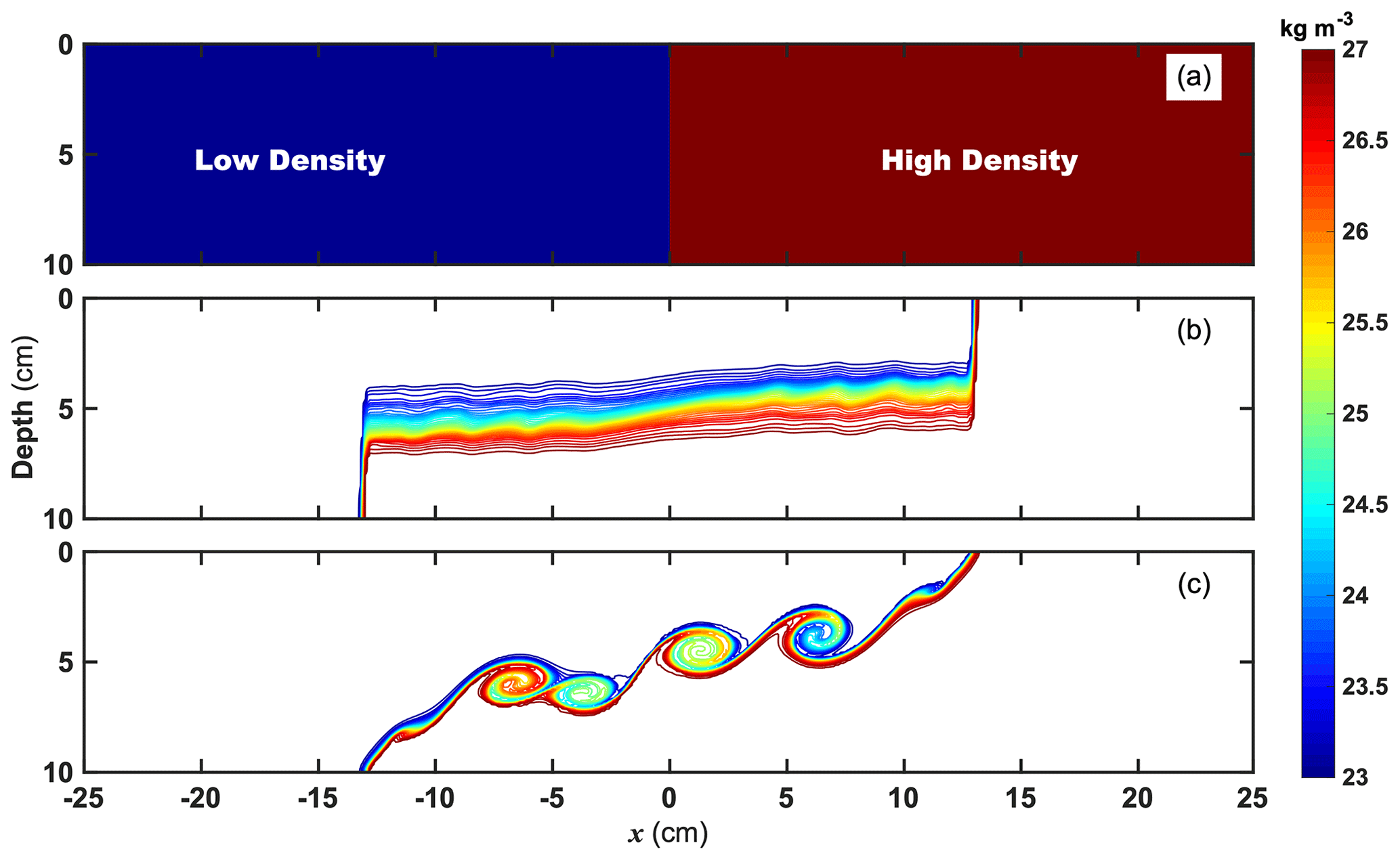
Figure 1 (a) The initial density σ (hereafter the same expression) field of the lock-exchange case and contour plots of density at t=4.5 s, where the contour interval is 0.1 kg m⁻³ under the hydrostatic (a) and nonhydrostatic (b) model framework.

The proper boundary conditions need to be given to solve this Poisson equation (Eq. 27). Here, the homogeneous Neumann boundary condition at the solid boundaries, also called the zero-gradient condition (Eq. 29), is used with good compatibility with the no-flux normal to slope, where n is the normal unit vector (Marshall et al., 1997a). We assume that nonhydrostatic dynamic processes are weak enough at the sea surface and open boundaries. In other words, the input signals through the boundaries are dominantly hydrostatic with nonhydrostatic pressure perturbation close to zero. The nonhydrostatic dynamic framework is restricted to the interiors. Hence, the zero-gradient condition is utilized to hold back sharp nonhydrostatic pressure gradients at the open boundaries. With the above boundary conditions, this linear system (Eq. 28) can be solved via the Krylov subspace method with PETSc's assistance on parallel computers under the standard MPI-based framework (Balay et al., 2020). Also, a highly efficient method needs to be devised to precondition the huge and sparse matrix A. Here, the multigrid preconditioner (Smith et al., 1996) and flexible generalized minimal residual algorithm (Saad, 1993) are employed in numerical validation experiments in this paper to minimize computational costs.

3 Model applications and assessments

In this section, we present a series of ideal numerical validation experiments to explore the correctness and compatibility of nonhydrostatic algorithms together with ORCTM. In allusion to the internal solitary wave dynamics, these test cases range from laboratory-scale cases in an enclosed tank to field-scale ones like the northern South China Sea with open boundaries. The first case is the lock-exchange problem as the preliminary validation. The second to fourth cases are designed to explore the nonlinear evolution of internal solitary waves induced by their interactions with the changing terrain. The last one is the generated nonlinear internal wave case in a double-ridge environment analogous to the Luzon Strait, which aims at the generation and disintegration of nonlinear internal waves to examine the effectivity of the open tidal forcing condition module under the nonhydrostatic algorithms. Analyses of all test experiments above indicate that ORCTM can reproduce nonlinear and nonhydrostatic internal solitary waves in different oceanic environments, which shows the robustness and reliability of this nonhydrostatic ocean model.

3.1 The lock-exchange problem

When shear currents flow between two different density fluids, the Kelvin–Helmholtz instability (hereafter K-H instability) will appear to cause turbulent diapycnal mixing (Lawrence et al., 1991; Cushman-Roisin, 2005). The perturbation on the interface gradually develops and stimulates numerous small eddies due to energy dissipation. The magnitude order of vertical flow is comparable to the horizontal one, so the nonhydrostatic effect matters throughout the whole process. We set a rectangular enclosed tank separated by a vertical board in the middle at the x-axis origin. Both sides of the tank are separately filled with two different density fluids in Fig. 1a. The gravitational adjustment will proceed when the central board is disengaged just like a lock gate. Here, we refer to the previous configurations (Härtel et al., 2000; Fringer et al., 2006; Lai et al., 2010) as a 2-D problem. The horizontal length L is set to 50 cm, and the static water height is 10 cm without topographic change in the tank. The grid resolution is 0.001 m in the horizontal and vertical directions. Several sensitivity experiments were explored to reduce the dissipations out of solid boundary friction, so the bottom friction coefficients are finally set to zero; both A_V0 and D_V0 in Eqs. (11) and (12) are $\mathrm{2}\times {\mathrm{10}}^{-\mathrm{6}}$ m² s⁻¹. In addition, water density averages are calculated based on the prescribed salinity difference on the left and right sides of the tank: ρ_l=1023.05 kg m⁻³ and ρ_r=1026.95 kg m⁻³.

The K-H instability process grows rapidly with good eddy reconstruction and outstanding wave breaking. In contrast, in that model configuration, we also run the same configuration experiment above but under the hydrostatic balance scheme. Figure 1b and c show the results of density σ (define $\mathit{\sigma }=\mathit{\rho }-\mathrm{1000}$ kg m⁻³) at the same time under the hydrostatic and nonhydrostatic balance framework. The comparison proves that the K-H instability cannot proceed resulting from the inapplicability of the hydrostatic balance. The perturbation on the density interface is so tiny that the density fronts cannot evolve in the upper and lower layer, so the mixing caused by the overturning and shear is too weak to be seen. On the contrary, via the nonhydrostatic scheme, the eddies can proliferate with energy dissipation due to the associated shear on the perturbation, vigorously mixing the high- and low-density water on the interface. More specifically, the energy is transmitted to the small-scale eddies across the density fronts due to dispersion and nonlinearity.

The evolution process of K-H instability is shown in Fig. 2. It is out of gravitational adjustment that the density front movement is accompanied by heavy water in the bottom and light water in the upper level moving to the left and right, respectively, causing a velocity shear field and clockwise rotating interface in Fig. 2a. The shear strength gradually increases until breaking the critical point of restoring force that depends on the density gradient, and later a series of eddies grows from the middle to both sides of the tank with the turbulent rolling and overturning. These eddies mix the water body with high density at the bottom and the upper one with low density, forming multiple considerable density mixing areas in Fig. 2b and c. When the bottom density flow is reflected on the left wall, a similar adjustment process begins to develop in reverse of Fig. 2d and e, but the strength of subsequent eddies is significantly weakened due to energy dissipation.

Figure 2 Density field evolution at t= (a) 5.0, (b) 7.5, (c) 10.0, (d) 12.5, and (e) 15.0 s.

These density distributions display the generation of density fronts and numerous eddies throughout the gravitational adjustment process. Based on the point of energy dynamics, the gravitational potential energy (PE) is converted to kinematic energy (KE) for the water parcel, while the total energy dissipates continuously in the tank. Here, KE and PE of the entire 2-D tank are calculated from the following formulas.

$$\begin{array}{}\text{(30)}& {\displaystyle }\mathrm{KE}=\underset{\mathrm{0}}{\overset{L}{\int }}\underset{-H}{\overset{\mathit{\varsigma }}{\int }}{\displaystyle \frac{\mathrm{1}}{\mathrm{2}}}\mathit{\rho }\left(u^{\mathrm{2}}+w^{\mathrm{2}}\right)\mathrm{d}x\mathrm{d}z\text{(31)}& {\displaystyle }\mathrm{PE}=\underset{\mathrm{0}}{\overset{L}{\int }}\underset{-H}{\overset{\mathit{\varsigma }}{\int }}\mathit{\rho }gz\mathrm{d}x\mathrm{d}z\end{array}$$

The three curves show the fluctuation of PE, KE, and total energy during the K-H instability simulation in Fig. 3. The PE and KE correspond to the maximum and zero due to the initial density distribution and static field in Fig. 3a. Afterward, the PE declines sharply with an opposite change in KE. Both rates of change are almost the same based on the curve slopes, which demonstrate that PE is converted to KE, reaching mutual peaks of about 9.5 s at the end of the first gravitational adjustment. From then on, both of them still maintain the opposite trends with an oscillation of roughly 25 s. It is worth noting that all kinds of energy exhibit a downward trend, with their oscillation period increasing steadily due to energy dissipation so that KE will drop to zero, and PE and total energy (PE + KE) will reach constant values in the end. The results above are equivalent to previous works (Härtel et al., 2000; Fringer et al., 2006; Lai et al., 2010), implying the correctness of the nonhydrostatic dynamic module.

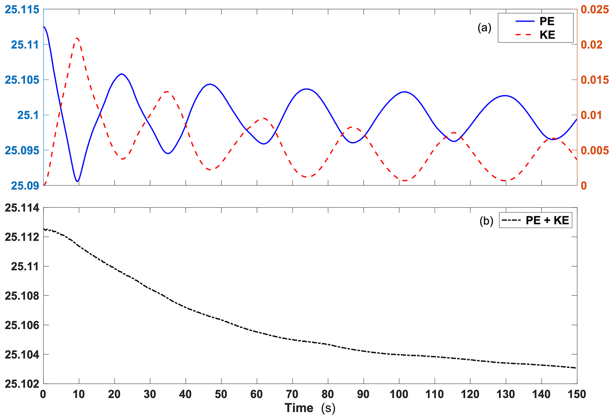
Figure 3 (a) The time series of kinematic energy (red dashed line), potential energy (blue solid line), and (b) total energy (black dotted line) (units: kg m² s⁻²).

3.2 Internal solitary wave in a tank

Internal solitary wave activities are ubiquitous in the ocean, with strong nonlinearity and nonhydrostatic effects. Laboratory experiments are usually carried out to study the ISWs to make up for the deficiencies of field observations. Numerical ISW experiments in a laboratory-scale background need to be combined simultaneously (Grue et al., 2000). We follow the previous experimental configuration (Ma et al., 2020). A schematic diagram of the ISW experiment is given in Fig. 4. The tank length is 2.0 m with the x-axis origin located on the left; the static height is 10 cm without topographic change; the horizontal and vertical resolutions are $\mathrm{2}\times {\mathrm{10}}^{-\mathrm{3}}$ and $\mathrm{1}\times {\mathrm{10}}^{-\mathrm{3}}$ m; both bottom friction and drag coefficients are set to $\mathrm{3}\times {\mathrm{10}}^{-\mathrm{3}}$ with the effect of a fairly robust friction to the ISW; A_V0 and D_V0 are the same as in the experiment configuration in Sect. 3.1. Here, a gravity collapse method is used to generate the depression ISW. Specifically, the low- and high-density fluids initially fill the upper and lower layers of the tank with the collapse area on the left side. The collapse height and width are 5.0 and 4.0 cm. Water density averages are calculated in the upper and lower layer with ρ₁=1003.62 kg m⁻³ and ρ₂=1026.95 kg m⁻³. Additionally, a diagnostic module is employed to characterize the high-frequency variation. The high-frequency outputs are positioned at points x=0.4, 0.8, 1.2, and 1.6 m with a time interval of 0.05 s.

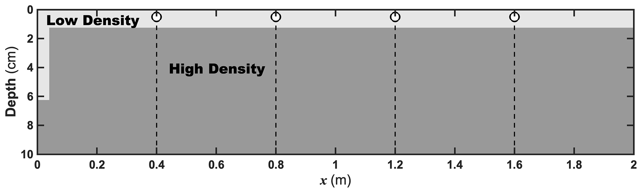
Figure 4 Schematic diagram of the ISW case. The light and dark gray indicate the low- and high-density water with 1003.62 and 1026.95 kg m⁻³; four white dots refer to the high-frequency output points.

Figure 5 distinctly illustrates the evolution of the ISW packet in the tank based on the pycnocline fluctuation. The isopycnic of 1026 kg m⁻³ can characterize the maximum strength of the depression ISW in Fig. 5a. The eastward starting wave packet originating from the west gravity collapse area comprises the depression heading wave and several tail waves whose amplitudes decrease successively. The heading wave with the maximum amplitude propagates much faster than the tails behind so that the distance expands promptly between them. As shown in Table 1 about the heading wave characteristics at the four locations, we find the wave amplitude with almost little change and then a slight fluctuation but no more than 0.1 cm after x=0.8 m. The quantitative evaluation of the wave speed based on the slope of the blue dashed area in Fig. 5b reveals that the wave speed increases slowly after x=0.2 m but with its increment less than 0.01 m s⁻¹. This indicates that the starting ISW packets are still at the stage of gravity adjustment before arriving at x=0.2 m and then propagating to the east steadily in our simulation. Also, the characteristic westward-reflected waves (the blue line in Fig. 5a) with the larger amplitude prove that wave–wave interactions happen between the reflected and starting tail waves.

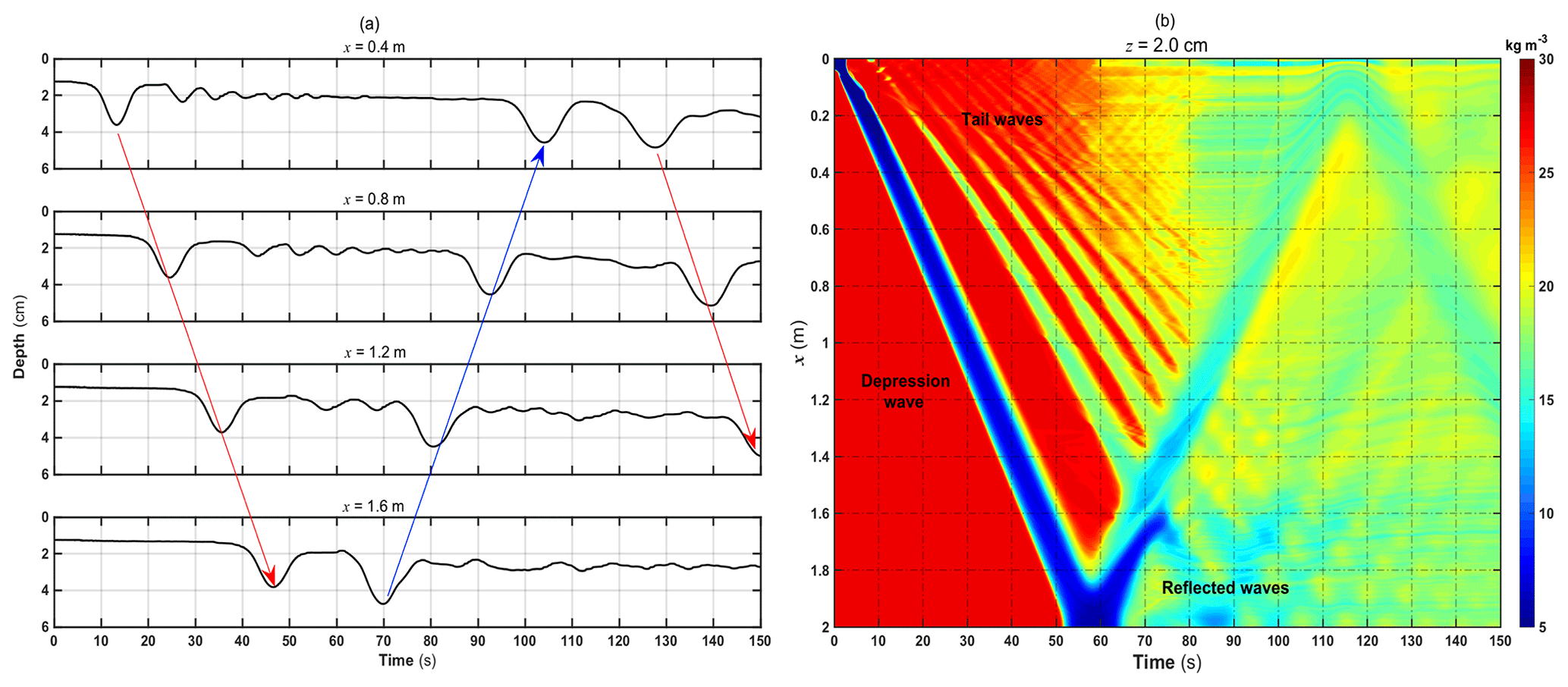
Figure 5 (a) The density time series of 1026 kg m⁻³ at the four high-frequency output locations from the west to east. The left red and blue arrow lines indicate the eastward and westward waves, and the right arrow line after 120 s indicates the eastward-reflected waves from the channel start. (b) Hovmöller diagram showing the density σ at z=2.0 cm, where the time interval is 0.1 s.

Table 1 The characteristics of the depression heading wave at the four points.

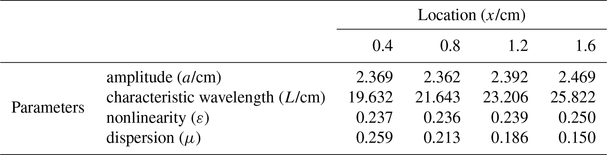
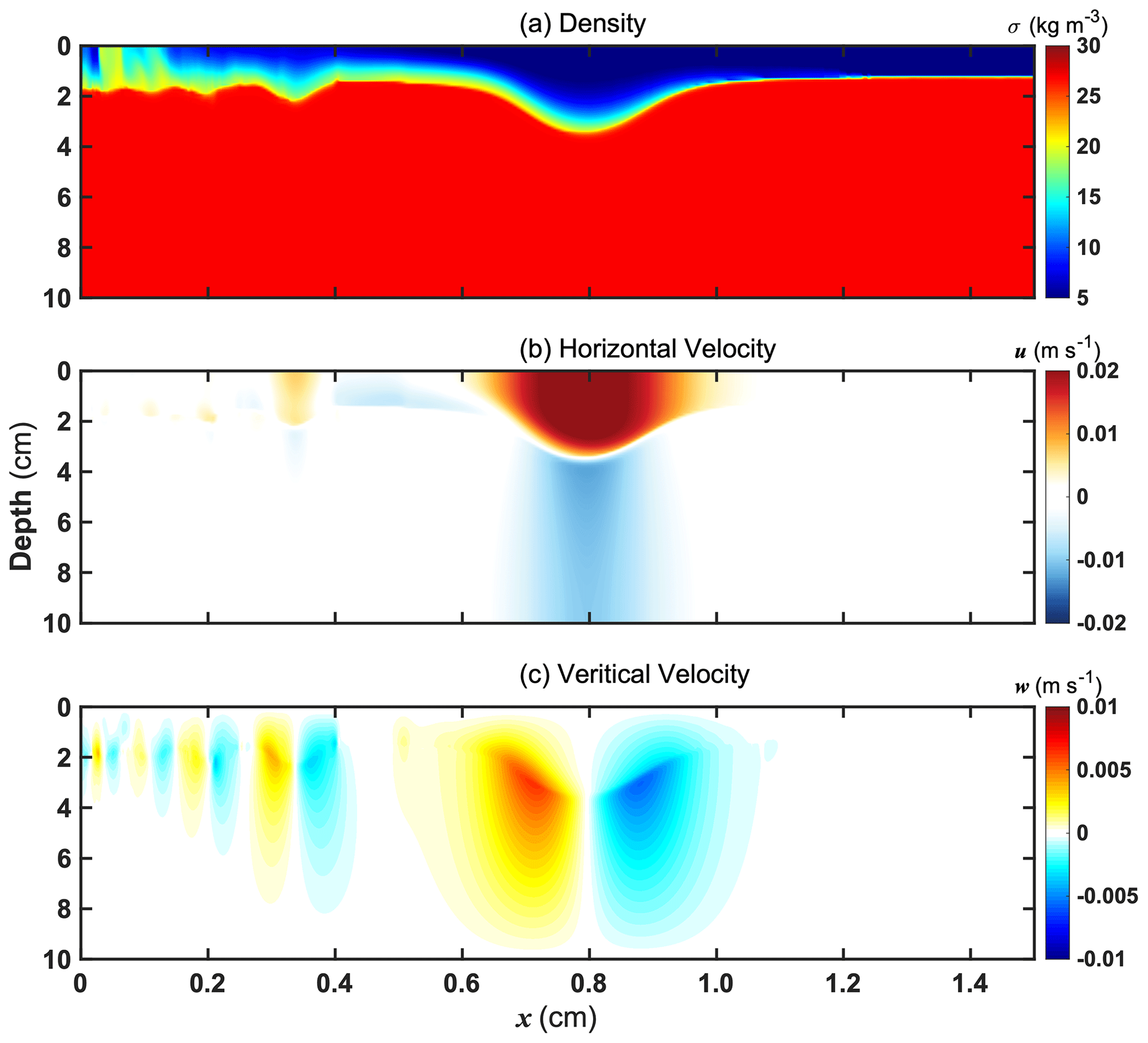
Figure 6 From top to bottom: density as well as the horizontal and vertical velocity fields of the ISWs at t=24.5 s.

We select a snapshot result for characteristic verification shown in Fig. 6 when the heading wave arrives at around x=0.8 m. The strongest horizontal velocity of the depression wave is 0.023 m s⁻¹, and the vertical flow can reach up to 0.0065 m s⁻¹. The characteristic velocity fields are in line with the clockwise structure of a theoretical depression internal solitary wave. Furthermore, the nonlinearity $\mathit{\epsilon }=a/h$ and dispersion $\mathit{\mu }={\left(h/\mathit{\lambda }\right)}^{\mathrm{2}}$ are calculated at the different locations in Table 1, where a, h, and λ are the amplitude, water height, and characteristic wavelength. The KdV (Korteweg–de Vries) model (Benjamin, 1966) described in Appendix B is utilized to predict theoretical waveforms at the four locations. The comparison depicted in Fig. 7 demonstrates that the results are more consistent with the KdV model than the m-KdV (modified KdV) model. According to the nonlinearity ε from Michallet and Barthélemy (1998), small- and large-amplitude ISWs can be classified when ε<0.05 and ε>0.05, respectively, whereas the application of the KdV model requires a balance between weak nonlinearities and dispersion (Ono, 1975), which namely needs to satisfy this condition: $\mathit{\mu }=O\left(\mathit{\epsilon }\right)\ll \mathrm{1}$. Despite the large-amplitude waves simulated from our model with ε>0.05, the nonlinearity and dispersion are of the same order and small enough that the heading wave can be deemed under weak nonlinearity. This can explain why the waveforms are better described by the KdV model. Therefore, analyses of the theoretical model indicate that the simulation of internal solitary waves can be fulfilled authentically using our nonhydrostatic model.

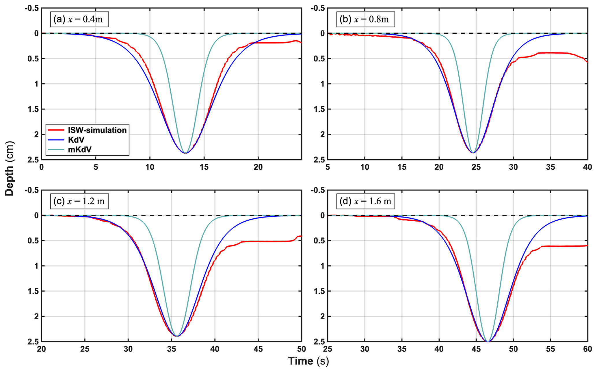
Figure 7 The interface displacement induced by heading ISW at four high-frequency output locations. The red lines indicate the 1026 kg m⁻³ isopycnic, and the blue and cyan lines represent the KdV and m-KdV model results.

3.3 Internal solitary wave shoaling on a Gaussian terrain

Based on the experiment configuration in Sect. 3.2 (also called Exp. 3.2), a slowly varying terrain is implemented to explore the nonlinear evolution of internal solitary waves in Sect. 3.3 (also called Exp. 3.3), especially the wave shoaling. As shown in Fig. 8, the left half of the Gaussian curve is reserved as the slope-shelf terrain starting between x=1.0 and 1.3 m with a height of 5.0 cm, and then the water depth remains unchanged from x=1.3 to 2.0 m corresponding to the shallow-water zone. High-frequency outputs are acquired during the climbing process of ISWs at points x=0.4, 0.8, 1.0, 1.2, 1.3, 1.4, 1.6, and 1.8 m with the same output interval as Exp. 3.2.

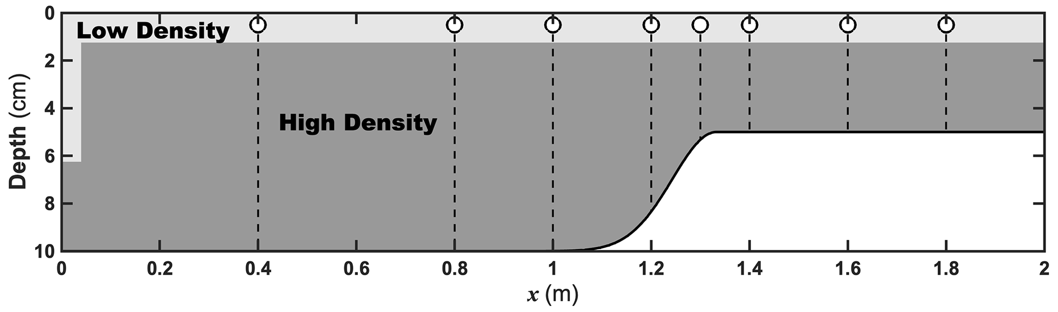
Figure 8 As in Fig. 4, but with half-Gaussian topography in the east of the tank; eight white dots refer to the high-frequency output points.

The evolution of internal solitary waves with varying topography is displayed in Fig. 9. The heading ISW holds a stable packet at x=0.4 m and initiates shoaling after reaching x=1.0 m. Afterward, the heading ISW undergoes topographic change so that the speed of the wave trough is less than the wave rear. Consequently, the contrasting effects on the wave front and wave rear contribute to the former gentle sloping but the latter gradual steepening, which shows a similarity with Vlasenko et al. (2002). Then the closed isopycnic contour mirrors the backward overturning and rolling due to the wave breaking at x=1.2 m in Fig. 9a. Apart from the wave breaking process above, it is also found in Fig. 9b that the reflected waves propagate back to the deep-water zone from x=1.2 m. In other words, both wave breaking and refection substantially attenuate the original depression ISW energy. When arriving east of x=1.2 m, the original depression wave is past the critical point where the upper layer is thicker than the lower one in Fig. 10a, so an elevation wave springs up in the wave rear. The elevation wave then continues to propagate eastward, which leads to increasing accumulation of high-density water in the upper water in the right region close to the wall of the tank. Hence, a new collapse area between x=1.8 m and the east wall comes into being where the thickness of the upper layer is larger than the lower layer. Ultimately, the westward-reflected waves, including a series of elevation tail waves, are released at x=1.6 m. In detail, the first elevation is the leading one with a rank-ordered structure in the rear. After reaching the deep-water zone left to 1.3 m, the wave rear begins to steepen and sink, and a depression wave forges behind the wave rear. Namely, the soliton wave passes the critical point inversely due to the wave deepening.

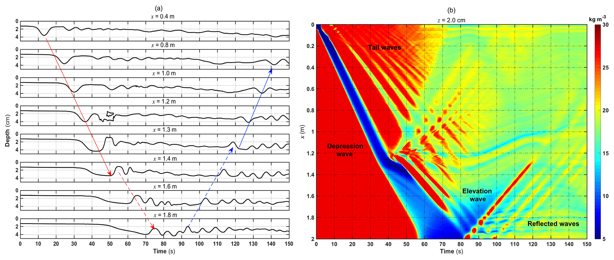
Figure 9 As in Fig. 5, (a) the solid and dashed arrow lines indicate the depression and elevation waves, and the red and blue mean the eastward and reflected westward waves. (b) Hovmöller diagram showing the density σ at z=2.0 cm.

Figure 10 The shoaling of a depression soliton with the velocity fields (black arrow) and the vorticity results (color) shown at t= (a) 35, (b) 40, (c) 45, (d) 50, (e) 55, and (f) 60 s.

For further exploration of the evolution of the depression wave, the distributions of the vorticity $(\mathit{\zeta }=\partial w/\partial x-\partial u/\partial z)$ with velocity vector are depicted in Fig. 10. The depression wave core features negative vorticity with an anticyclonic velocity structure before reaching the shelf topography. When the ISW approaches the top of the slope in Fig. 10a and b, the vertical shear increases promptly and strengthens the positive vorticity at the bottom. Then the backward overturning springs up between x=1.2 and 1.3 m, marking the ISW entering the breaking instability stage (Helfrich and Melville, 1986) due to the shoaling. At this time, even though wave breaking and reflection render partial wave energy dissipation, a fraction of the depression wave can reach the shallow-water zone, leaving a cyclonic vortex behind above the slope shelf in Fig. 10c. This partial soliton wave is adjusted instantaneously when the upper layer thickness is more significant than the lower in light of the boundary of the negative vorticity area in Fig. 10d. As a result, after the reverse situation occurs, the elevation wave begins to emerge at the back of the original wave. Its core corresponds to the positive vorticity with a cyclonic velocity structure. In addition, the vortex from the wave breaking weakens slowly and motivates numerous small-scale waves with high wavenumber propagating to both sides in Fig. 10e and f, which is consistent with the propagation characteristics of the reflected waves near x=1.2 m in Fig. 9b.

It is also worth highlighting the evolution of the reflected westward waves. We also visualize the process of the second reverse situation due to the wave deepening in Fig. 11. It can be noticed that there is a leading elevation wave at x=1.4 m followed by a series of rank-order waves exhibiting a likewise sinusoidal variation. They propagate together to the deep-water zone with the wave crest corresponding to positive vorticity. Particularly, the wave train is considered approximately linear based on the alternating positive and negative vorticity regions, since the cores of these waves are located almost in the middle layer where the nonlinear parameter α is close to zero in terms of the KdV model. As the water depth becomes deeper, the crest of the elevation wave gradually grows down and flattens with the wave rear sinking. The original elevation cannot be maintained in the deep water, transforming into a depression wave with the velocity fields adjusted accordingly.

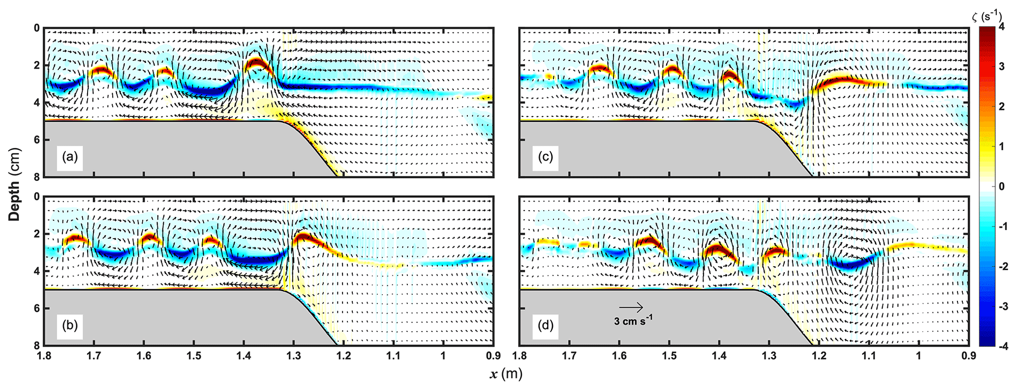
Figure 11 As in Fig. 10, the elevation wave propagates westward to the deep water; the x axis is inverse for convenience at t= (a) 115, (b) 120, (c) 125, and (d) 130 s.

The ISW is not stable enough to coincide with the KdV model after passing the critical point into the adjustment stage. Hence, we select the two types of soliton results for verification before the reverse situation occurs. The comparison results between theoretical and numerical model are illustrated in Fig. 12 at x=0.8 and 1.4 m before the wave shoaling and deepening, respectively. We can find that the depression waveform conforms to the KdV model results before climbing the slope, whereas the elevation is closer to the m-KdV model. Compared with ε=0.233 at x=0.8 m, the interaction between the ISW and the shoaling topography renders a stronger nonlinearity (ε=0.331) of the elevation heading wave in the shallow water. Namely, the larger wave amplitude ratio in the shallow-water results can be characterized with m-KdV theory, which compares well with the conclusions of Michallet and Barthélemy (1998) in a satisfactory way.

Figure 12 Wave profiles at x=0.8 (a) and 1.4 m (b). The left (right) refers to the depression (elevation) heading wave before shoaling (deepening); the results are plotted with the red line. The blue and cyan lines represent the KdV and m-KdV model results.

3.4 Internal solitary wave breaking on a slope.

To further characterize a complete breaking and dissipative process of ISWs, we set a linear slope identical to Michallet and Ivey (1999). As is shown in Fig. 13, the tank length is 2.0 m; The height is 15 cm with the linear terrain placed on the east side. The model configuration (i.e., spatial resolution and viscous coefficients) is identical to Exp. 3.2, which can ensure the same time step according to the Courant–Friedrichs–Lewy (CFL) condition, and the depression ISW is about to be dissipated due to increasing bottom friction at the shelf break. In contrast with Bourgault and Kelley (2004), water density averages are calculated to be ρ₁=1000.01 kg m⁻³ and ρ₂=1047.00 kg m⁻³ in the upper and lower layers. Via several sensitivity experiments about collapse area, the amplitude of the depression wave can reach approximately 2.8 cm when the collapse height is 9.0 cm with its width identical to Exp. 3.2. Although the stimulated wave strength is slightly greater than the results from Bourgault and Kelley (2004) due to the different wave generation methods, it is predictable that the breaking of the larger-amplitude ISW will be more dramatic with a prominent performance for model verification.

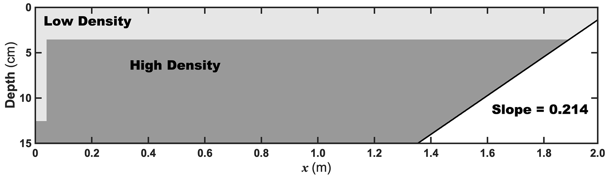
Figure 13 As in Fig. 4, the low and high densities are set to 1000.01 and 1047.00 kg m⁻³ with a linear slope terrain placed in the east of the tank; for the related configuration, refer to Bourgault and Kelley (2004).

The associated density and velocity fields produced by the depression ISW are presented in Fig. 14 at t=15 s before wave shoaling. The horizontal velocity is about 3.0 cm s⁻¹ at the surface and varies up to 3.5 cm s⁻¹ at the wave core. Meanwhile, the vertical velocity distribution presents a double-core structure reaching ±0.8 cm s⁻¹. The unique anticyclonic velocity characteristic just like an eastward rolling wheel is consistent with the model results of Bourgault and Kelley (2004). We select the four moments of the evolution of wave shoaling illustrated in Fig. 15. In addition to wave breaking accompanied by the waveform steepening in the rear, a significant density front rolling in the wave front evolves along the linear slope during the overall shoaling process in Fig. 15a and b. Specifically, while the depression wave continues to get closer to the shallow zone, the effect of bottom friction can maintain the vertical shear and increase the potential energy, which intensifies the diapycnal mixing and dissipation on the density interface. Then the wave-induced diapycnal flow contributes to high-density water under the interface transported continuously to the shallow zone in Fig. 15c. On the other hand, there is another pronounced peculiarity in Fig. 15d compared to Exp. 3.2. A few small-scale eddies emerge along with the sheared interface due to the shear instability.

Figure 14 As in Fig. 6, but with the time referring to t=15 s before the wave shoaling.

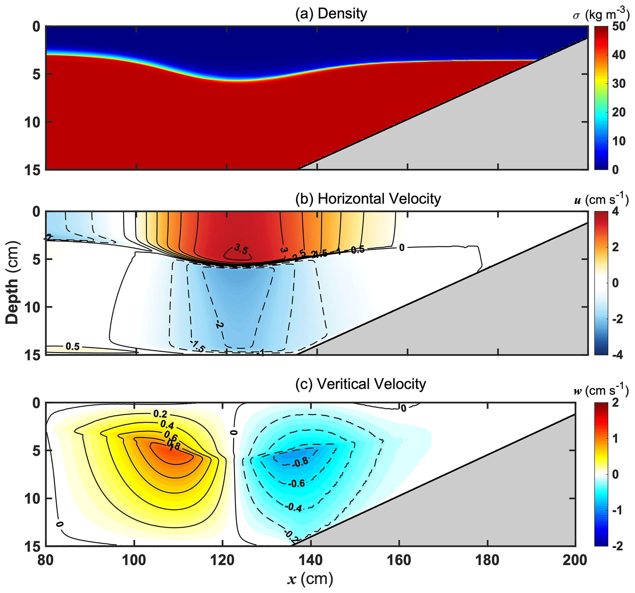
Figure 15 Wave breaking with density front rolling at t= (a) 22, (b) 23, (c) 24, and (d) 25 s.

To further evaluate and validate the wave breaking process, we compare the velocity field distributions with the observation results via PIV (particle image velocimetry) technology from Michallet and Ivey (1999) and nonhydrostatic numerical experiments from Bourgault and Kelley (2004) in Fig. 16. Accordingly, when the depression wave arrives over the slope, its depression waveform and anticyclonic flow field are modulated by the topographic shoaling to flatten the wave front and enhance the downward current along the slope due to the bottom friction. Meanwhile, a smaller cyclonic eddy appears and clings to the slope under the steepened wave rear in Fig. 16a. As the deformed depression wave persists in shoaling, the cyclonic eddy is reinforced and extends its scope of influence, resulting in a strong overturning from near the bottom layer to promote the wave steepening in Fig. 16b, which presents good agreement with the results from Exp. 3.3. Afterward, the anticyclonic flow structure has been ruined since bottom friction commences, hindering the current down the slope. In contrast, the coverage of the cyclonic eddy continues to expand and moves the shallow zone with the waveform distorted further. All the above nonlinear processes are similar to previous laboratory and model results. Our nonhydrostatic model can also resolve the nonlinear evolution of the internal solitary waves at shelf break with high enough accuracy.

Figure 16 Comparison of velocity fields during the wave breaking on a linear slope between (left) the PIV observations in the laboratory (Michallet and Ivey, 1999), (middle) the numerical model simulation (Bourgault and Kelley, 2004), and (right) ORCTM simulation at t= (a) 21.7, (b) 22.2, and (c) 23.2 s from top to bottom. The red contours indicate the isopycnic lines.

3.5 Nonlinear internal waves in a double-ridge system

The last validation experiment is to examine the generated nonlinear internal waves via tidal flow over the varying topography. We set up an underwater double-ridge system comparable to the Luzon Strait in the northern South China Sea (SCS), where the largest internal solitary waves in the world can exist (Huang et al., 2016). This validation case is a 2-D problem for the reduction of computational resources as well. The topography in this double-ridge system is fitted approximately with the Gaussian function given as

$$\begin{array}{}\text{(32)}& \begin{array}{rl}H\left(x\right)& =\mathrm{3000}-h_{\mathrm{w}}\times \exp \left(-{\left({\displaystyle \frac{x-x_{\mathrm{w}}}{\mathrm{20}\times {\mathrm{10}}^{\mathrm{3}}}}\right)}^{\mathrm{2}}\right)-h_{\mathrm{e}}\\ & \times \exp \left(-{\left({\displaystyle \frac{x-x_{\mathrm{e}}}{\mathrm{20}\times {\mathrm{10}}^{\mathrm{3}}}}\right)}^{\mathrm{2}}\right).\end{array}\end{array}$$

In Eq. (32), H(x) is the water depth; the height of the east ridge and west ridge (h_e and h_w) is 2500 and 1300 m in sequence with an interval and widths of 100 km, which is similar to the fundamental topographic characteristics in the Luzon Strait. As shown in Fig. 17a, the static water height is 3000 m; the east ridge and west ridge (hereafter ER and WR) are located at the coordinate origin and $x=-\mathrm{100}$ km; the horizontal and vertical grid resolutions are uniformly 200 and 10 m throughout; A_V0 and D_V0 in Eqs. (11) and (12) are set to $\mathrm{2}\times {\mathrm{10}}^{-\mathrm{4}}$ and $\mathrm{2}\times {\mathrm{10}}^{-\mathrm{5}}$ m² s⁻¹; the bottom friction coefficients are both $\mathrm{3}\times {\mathrm{10}}^{-\mathrm{3}}$. As for the tidal categories, the generation of semidiurnal ITs and the modulation effect of diurnal ITs in the Luzon Strait determine the evolution of the larger-amplitude ISW packet in the northern South China Sea (Buijsman et al., 2010a; Zeng et al., 2019), so we define the M₂ and K₁ tidal current amplitudes as 5.0 and 4.0 cm s⁻¹ corresponding to the semidiurnal and diurnal components at the open boundaries; the sponge thicknesses L_sp of the west and east boundaries are both approximately 40 km, and the timescale coefficient τ is set to 500 s. These model configurations in the validation experiment are analogous to the control test from Li (2014) and Zhang et al. (2011) to reproduce the major structures of NIWs in the South China Sea. In addition, to simplify the background environment, we also use horizontally uniform stratification as the initial field for our model. Here, the representative stratification in Fig. 17b to d stems from the GLORYS12V1 reanalysis product in CMEMS (Copernicus Marine Environment Monitoring Service). The initial field is based on the spatial mean around the source of generated ISWs in the Luzon Strait during the summer of 2011, since large-amplitude ISWs are observed during this period on the SCS continental shelf (Ramp et al., 2019) and the strong thermocline structure in summer is conducive to the formation of baroclinic tides in the Luzon Strait (Zheng et al., 2007; Buijsman et al., 2010b;). Additionally, the slope criticality γ (Gilbert and Garrett, 1989; Shaw et al., 2009) no less than 1 is usually essential with the formation of linear internal waves:

$$\begin{array}{}\text{(33)}& \mathit{\gamma }={\displaystyle \frac{\mathrm{d}H}{\mathrm{d}x}}/\sqrt{{\displaystyle \frac{{\mathit{\omega }}^{\mathrm{2}}-f^{\mathrm{2}}}{N^{\mathrm{2}}-{\mathit{\omega }}^{\mathrm{2}}}}},\end{array}$$

in which ω is the tidal angular frequency, N² is the buoyancy frequency squared, and the Coriolis parameter f is set to zero for the Earth's rotation, which is neglected due to the 2-D environment. Around the east ridge γ is always larger than unity regardless of the M₂ and K₁ tide, which means the east ridge belongs to the supercritical topography. Therefore, it is predictable to generate internal waves due to the interactions with barotropic flow over the east ridge. We run the model for 10 d from an initial static field. The diagnostic module is also used to characterize the high-frequency variation with the output interval of 1 min at $x=-\mathrm{250}$, −350 km.

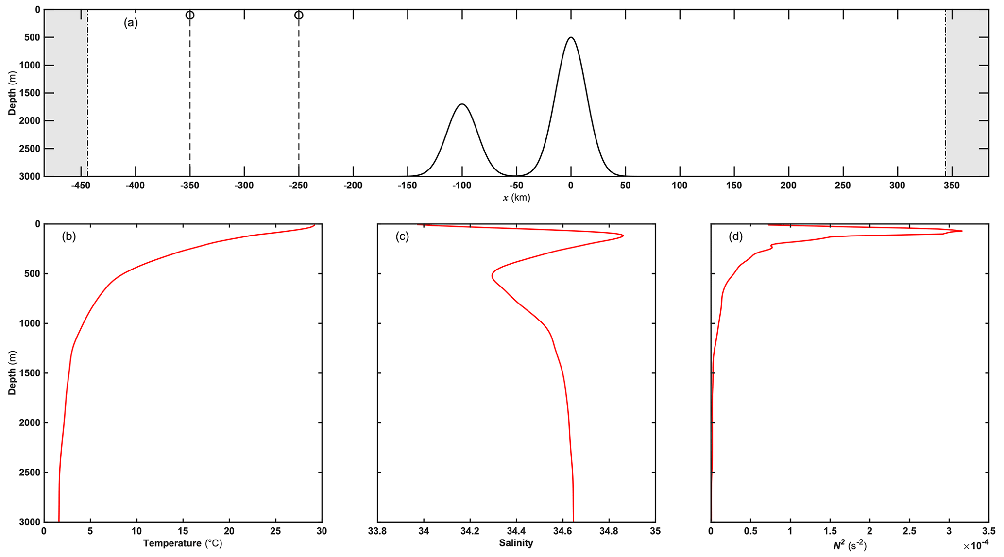
Figure 17 (a) A sketch of generated NIWs over the submerged double-ridge system case; the gray zones indicate the sponge layers. The summer stratification in 2011 including (b) temperature, (c) salinity, and (d) buoyancy frequency squared is from the spatial mean within 20.25–20.85^∘ N, 121.7–122.08^∘ E corresponding to the source of internal waves in the Luzon Strait (Zhang et al., 2011).

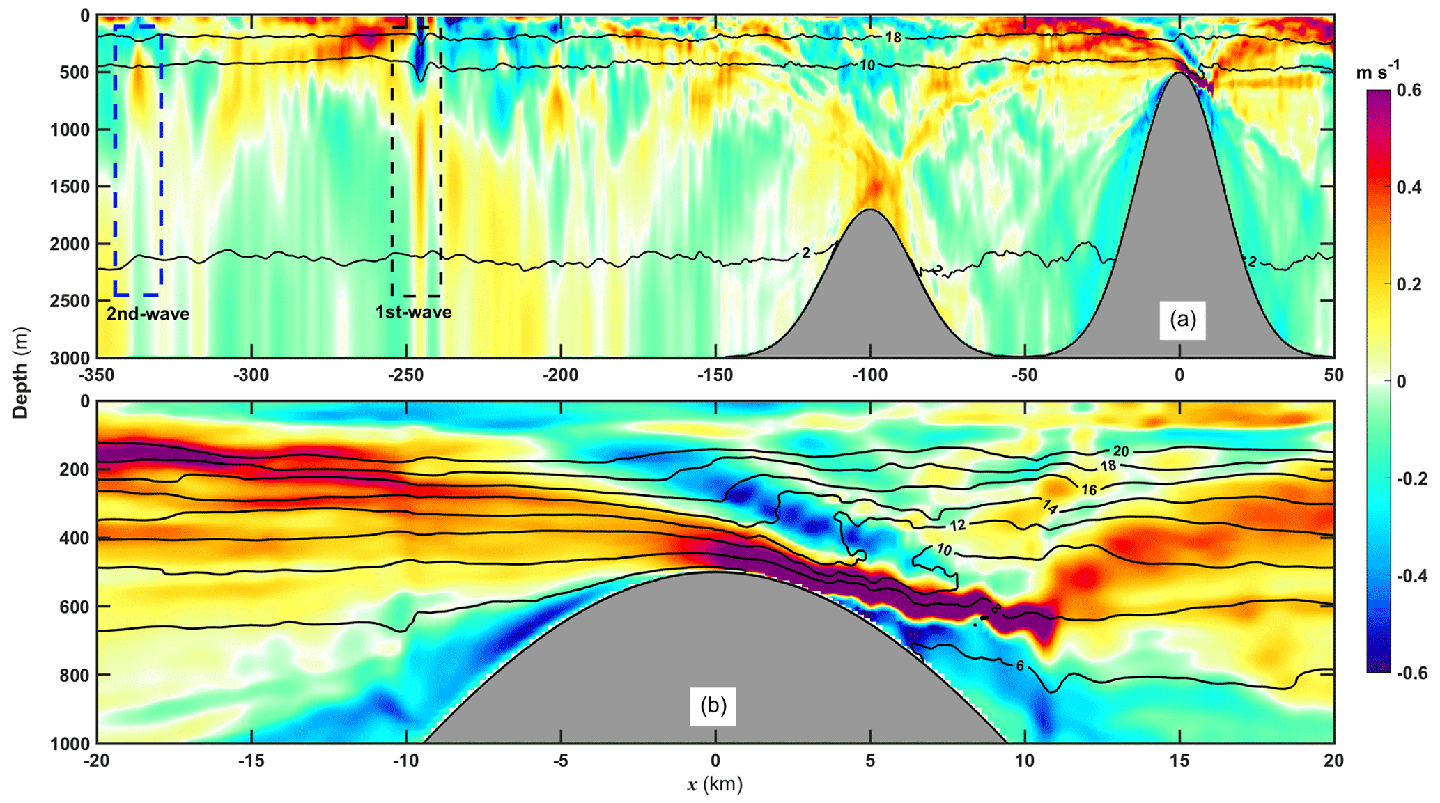
Figure 18 Distributions of horizontal baroclinic velocity with temperature (^∘C) contours for the western far field (a) and source field (b) when the maximum eastward tidal current at the east ridge reaches the end of ebb on the sixth day; the blue (black) dashed box means the second-mode (first-mode) ISW packets.

Figure 18 shows the maps of horizontal baroclinic velocity $u{}^{\prime }=u-U$, where u is the total velocity and U is the barotropic flow velocity. From the characteristics of the source field, the generation of an internal tide beam propagating eastward and westward centered from the eastern side of the east ridge is found. The eastward barotropic flooding current flows continuously over the east ridge with a maximum barotropic current up to 0.0531 m s⁻¹. A significant hydraulic jump can appear with the isotherm fluctuation up to roughly 200 m on the eastern side, which indicates the formation of lee waves to a certain extent. The above internal wave generation due to tide–topography interactions can be described with the below nondimensional parameters at the source: (1) the tidal excursion parameter $\mathit{\epsilon }=U_{\mathrm{0}}/L\mathit{\omega }$, which can be associated with the generation of an internal tide beam under critical or supercritical topography, where U₀ is barotropic current amplitude from the far field and L is the characteristic length for topography (Garret and Kunze, 2007; Chen et al., 2017); (2) the Froude number $Fr=U/c$ and its topographic form $F{r}_z=\mathit{\omega }/N(\mathrm{d}H/\mathrm{d}x)$, in which c is the mode-1 linear speed for the eigenvalue problem (Legg and Adcroft, 2003; see Appendix B). Specifically, Legg and Klymak (2008) found that the nonlinear hydraulic jump will develop with lee wave generation when $F{r}_z<\mathrm{1}/\mathrm{3}$. It is worth noticing that the tidal excursion far less than unity agrees with the formation of the linear internal tide beam on the critical or supercritical topography but cannot ensure the formation of lee waves altogether. For instance, the lee waves remain strong in the Luzon Strait despite the tidal excursion under unity (ε≈0.4) in previous model results (Buijsman et al., 2010b). The tidal excursion parameter ε and the Froude number Fr are estimated to be 0.025 and 0.018 in Fig. 18. That demonstrates that the multi-modal baroclinic tides and upstream propagation of internal waves will generate around the source field when the subcritical barotropic current flows over the east ridge. Furthermore, the maximum topographic Froude number is just 0.3362 around the east ridge with the approach to the regime transition value $\mathrm{1}/\mathrm{3}$, which ensures that the nonlinear hydraulic jump can grow with lee waves on the east of the east ridge. All of the above can explain the generation of the internal tide beam and hydraulic jump well in our simulation and confirm the mixed tidal lee wave regime in the Luzon Strait (Chen et al., 2017).

After the westward internal tide beam emitting from the east ridge reaches the sea surface and reflects into the deep sea, the partial downward internal tide beam can propagate to the top of west ridge below 1500 m depth and reflect into the upper layer again. Between the double ridges, such a significant portion of beam energy captured by the pycnocline waveguide together with the upstream influence can strengthen the westward-propagating internal wave energy in Fig. 18b, which can trace back to the source of the internal solitary wave packets in the far field. However, the strong dissipation for the high modal internal waves contributes to the vanishing of the internal tide beam structure and allows the nonlinear evolution of low-mode baroclinic tides. The low modal internal solitary wave packets can grow and propagate westward from $x=-\mathrm{150}$ km, marking the disintegration of the multi-modal nonlinear internal wave energy. Specifically, the first-mode ISW packet emerges from $x=-\mathrm{250}$ to −200 km. Meanwhile, the second-mode ISW between $x=-\mathrm{350}$ and −300 km performs the convex wave packet.

Figure 19 Hovmöller diagram about the global temperature time series at z=400 m, where the time interval is 15 min. The black solid curve indicates the tidal current at the east ridge, and the blue solid line means the west ridge location. The black and magenta dashed lines are the first- and second-mode internal solitary waves.

We can acquire the propagation characteristics of these ISWs via analyzing the global temperature time series at 400 m depth. As is illustrated in Fig. 19, the second-mode ISW packet propagates slower, and its strength is much weaker than the first-mode wave one. Also, it can be determined that the two first-mode wave packets can propagate westward in 1 d, one of which is stronger with the structure of several tail waves, and the other is almost solitary and weak. These two types of first-mode wave packets refer to type-a and type-b waves (hereafter a-wave and b-wave), respectively, in the northern South China Sea (Ramp et al., 2004). In addition, their occurrence time can be connected to the ebb of the eastward flood current around the east ridge. These simulated results in the strength and timing prove that a- and b-waves originate from the double ridge in Luzon Strait (Ramp et al., 2004, 2019; Zhao and Alford, 2006). Additionally, the relatively weak second-mode concave wave can be found distinctly following the a-wave from the west of −300 km. To sum up, the multi-modal baroclinic tide structures from the double-ridge system can propagate to the far fields. The low-mode internal waves gradually perform the corresponding ISWs due to nonlinear enhancement, which displays good agreement with the other two-dimensional experimental results (Buijsman et al., 2010a, b; Vlasenko et al., 2010).

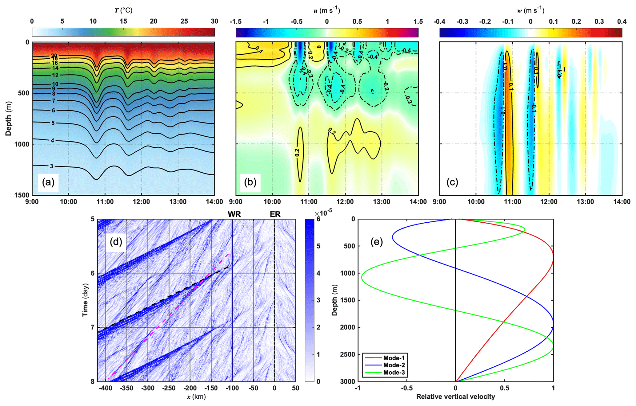
Figure 20 (a) The temperature (^∘C), (b) horizontal baroclinic velocity (m s⁻¹), and (c) vertical velocity (m s⁻¹) structures of the first-mode ISW packet at $x=-\mathrm{250}$ km on the sixth day. (d) The SSHG Hovmöller diagram during the associated period, with the black and magenta dashed lines indicating the first- and second-mode ISW packets. (e) The normal-mode profiles of vertical velocity for the first three modes using the Taylor–Goldstein equation.

To evaluate the comparison between the numerical ISWs with internal wave theory, we select the results of the first-mode ISW at $x=-\mathrm{250}$ km. In Fig. 20, it is found that a first-mode ISW packet including three tail waves arrives at the position after 10:00 on the sixth day. The maximum fluctuation of the first-mode ISW packet can reach 206 m located between 650 and 900 m water depths. The westward horizontal baroclinic velocity associated with the wave packet prevails above 200 m with a maximum strength of roughly 1.41 m s⁻¹, and the corresponding downwelling region is located between 200 and 1500 m depths with the strongest downward velocity up to 0.22 m s⁻¹. According to the sea surface height gradient (SSHG, SSHG is defined $\sqrt{(\mathrm{\nabla }\mathit{\varsigma }{)}^{\mathrm{2}}}$) in Fig. 20d, the average propagation speed of this wave packet is approximately 3.17 m s⁻¹ based on the slope of the SSHG contour. Moreover, we solve the Taylor–Goldstein equation (Miles, 1961; Liu, 2010; see Appendix B) 10 min before this wave packet reaches $x=-\mathrm{250}$ km, and the normal mode of vertical velocity is subject to the rigid-lib boundary condition. We found that the location of the maximum modal function is 710 m, in agreement with the model results in Fig. 20e. However, the propagation speed is greater than the first-mode linear result of 2.69 m s⁻¹, which is probably attributed to the underestimated effect in linear theory. Therefore, the KdV model is also utilized to analyze the depression wave packet. The nonlinear and dispersion parameters are $-\mathrm{3.4}\times {\mathrm{10}}^{-\mathrm{3}}$ s⁻¹ and 2.4×10⁵ m³ s⁻¹, which indicates that the theoretical depression wave is consistent with the simulated results (Helfrich and Melville, 1986). Nevertheless, the theoretical nonlinear velocity of about 2.88 m s⁻¹ is slightly lower than the simulated results. It is probable that the increasing nonlinearity with the steepening of internal tides ultimately leads to the larger propagation speed of this first-mode ISW packet.

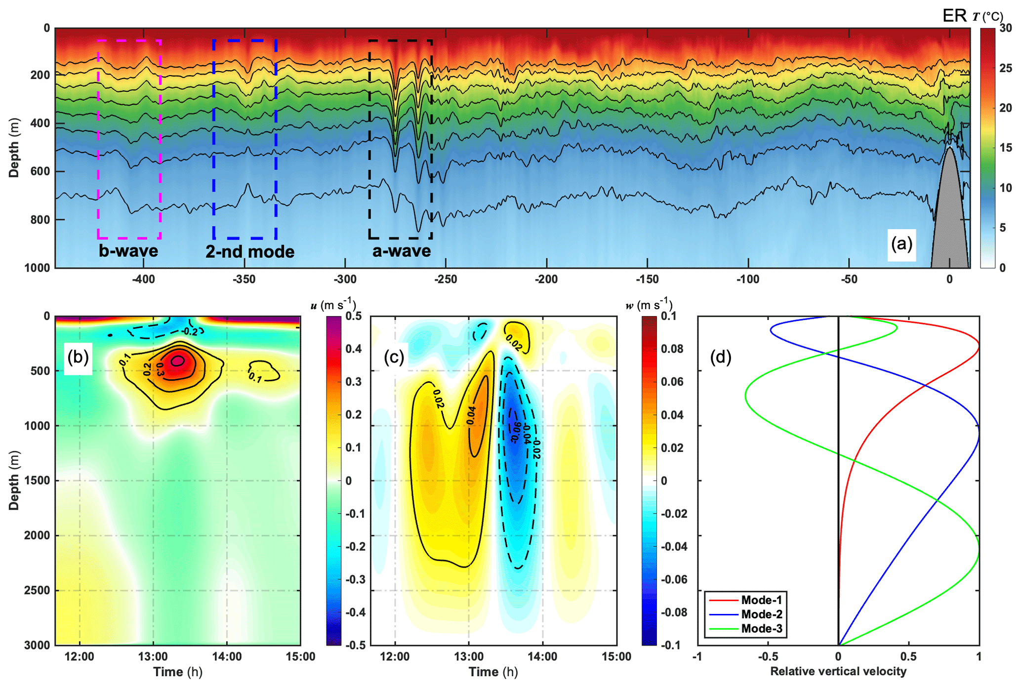
Figure 21 (a) The temperature (^∘C) field from the west side of the east ridge at 13:00 on the seventh day; dashed rectangles refer to the respective wave types. (b) The horizontal baroclinic velocity (m s⁻¹) and (c) vertical velocity (m s⁻¹) structures of the second-mode ISW at $x=-\mathrm{350}$ km. (d) The normal-mode profiles about vertical velocity for the first three modes using the Taylor–Goldstein equation.

It is also noticeable that the multi-modal internal solitary wave field is generated and strengthened gradually due to nonlinear enhancement. In Fig. 21a, we can recognize the distinct ISW packets from the isotherm displacement that refers to type-a waves, second-mode waves, and type-b waves from the source to the far field. The a-wave packet features the most substantial strength with tail waves when its vertical excursion induced by the heading wave can reach up to 120 m. In contrast, the weaker b-wave contains one depression soliton in the west to $x=-\mathrm{400}$ km. They both originate from a multi-modal internal tide caused by the tide–topography interactions in the double-ridge system, but the b-wave is more associated with the west ridge (Buijsman et al., 2010a; Zeng et al., 2019). Between a- and b-waves, there is a second-mode ISW packet evidently classified as having the structure of a concave wave whose upper and lower isotherms fluctuate downward and upward. The maximum isotherm fluctuations are located in roughly 180 and 1000 m depths and can reach up to −57.2 and 140.6 m. The propagation speed of this second-mode ISW is about 1.36 m s⁻¹ from the SSHG slope in Fig. 20d. It is predictable that the a-wave packet will follow the second-mode signal due to the more considerable speed. Figure 21b and c show the second-mode ISW packet and related velocity field time series at $x=-\mathrm{350}$ km. The horizontal baroclinic velocity field has a sandwich-shaped vertical structure, and the maximum of 0.42 m s⁻¹ is located in the middle layer between 200 and 600 m. The strength of baroclinic velocity with a small average of 0.2 m s⁻¹ is distinct from the stronger first-mode ISW packet above 200 m. Additionally, a double-peak structure performs in the vertical velocity field, and it is distributed at the depths of 150 and 1000 m where the strength in the deep layer is stronger than the upper, resulting in a minor isotherm fluctuation above 200 m. Here, the Taylor–Goldstein equation is also solved to acquire the eigenfunction of the vertical velocity. In Fig. 21d, the second-mode eigenvalues have two vertical peaks whose depths correspond to 150 and 1070 m, with the latter strength stronger than the former, and the corresponding phase speed is about 1.34 m s⁻¹. In summary, first- and second-mode internal solitary waves as the leading carriers can transfer baroclinic tidal energy from the source to far fields until dissipating thoroughly. The multi-modal solitary wave field conforms with the previous two-ridge experimental result using MITgcm (Vlasenko et al., 2010). Internal wave theoretical models can compare well with the distribution of stimulated results in our nonhydrostatic ocean model, demonstrating an overall good performance of characterizing the nonlinear evolution of multi-modal baroclinic tides.

4 Discussion and conclusion

The main focus of this paper is to introduce a new oceanic regional nonhydrostatic circulation and tide model (ORCTM) which is rooted from the MPI-OM and aims to characterize the internal solitary wave processes of real oceans, such as in the northern South China Sea. We developed and implemented the nonhydrostatic dynamics and open boundary module under the original global hydrostatic framework of MPI-OM. Based on the fractional step and finite-difference methods, ORCTM involves the three-dimensional fully nonlinear momentum equations under the Boussinesq fluid. The three-dimensional Poisson equation subject to different boundary conditions needs to be solved before the pressure correction method is employed to acquire the velocity field corrected via nonhydrostatic pressure gradient force. In order to match the nonhydrostatic algorithm and realize larger-amplitude ISW simulations in an ocean-scale case, an exponential relaxation term is implemented to the control equations through the sponge layers as the open boundary condition.

A series of two-dimensional ideal numerical experiments associated with the nonlinear evolution of the internal solitary waves and baroclinic tides is devised to verify this nonhydrostatic ocean model. Here, the results of the validation experiments are in accord with the theoretical framework of the nonhydrostatic dynamics and demonstrate that ORCTM can successfully characterize the generation, propagation, and dissipation of internal solitary waves in laboratory-scale cases. Specifically, the reverse situation due to wave shoaling and deepening can be depicted completely when considering the topographic change. Meanwhile, the stimulated internal solitary wave conforms with the previous numerical experiment and the direct observations in the laboratory test. Also, ORCTM can capture the density fronts with the cyclonic eddy induced by the wave breaking, which shows good stability and high enough accuracy. Furthermore, based on the real topographic features in the Luzon Strait of the northern South China Sea, analyses of the validation experiment indicate the multi-modal structure of baroclinic tides in the double-ridge system. The nonhydrostatic ocean model ORCTM is proven to be able to reproduce the life cycle of multi-modal ISWs induced by tide–topography interactions in the Luzon Strait and precisely capture the alternation process of type-a and type-b internal solitary wave packets. The first two-mode ISW structure compares well with the internal wave theoretical model.

Even though these validation experiments have a strong resemblance to other nonhydrostatic model results (Bourgault and Kelley, 2004; Berntsen et al., 2006; Lai et al., 2010), some distinctions in grid structure or numerical methods may have an opposite impact, especially when predicting a particular nonhydrostatic dynamics process. Berntsen et al. (2006) indicated some noisy structures near the bottom layer due to numerical errors of finite-volume treatment when predicting internal solitary wave breaking via MITgcm (Marshall et al., 1997a, b). They found that the Bergen Ocean Model (BOM) can avoid this problem with a sigma coordinate, whereas MITgcm needs a high-order filter to suppress the noise. However, artificial flow usually emerges and has a negative influence on ISW breaking simulations due to internal baroclinic pressure errors in the sigma coordinate. These require model users to have a refined grid when encountering an area of changing topography. Compared to the nonhydrostatic unstructured grid finite-volume coastal ocean model (FVCOM) (Lai et al., 2010) and BOM (Berntsen et al., 2006), ORCTM is based on the finite-difference method and owns a Z coordinate, which has the capability to avoid the above errors. These numerical methods and validation experiments demonstrate that ORCTM is able to approach or reach an acceptable or better level for a nonhydrostatic ocean model for ISW simulation.

The simulation of internal solitary waves can mirror the macroscopic structure and assist with the implementation of in situ observations. It is noticed that the predictability of nonlinear internal wave characteristics relies on the model performance and external conditions such as realistic stratification, bathymetry, and background circulation. Another advantage of ORCTM is the usage of an orthogonal curvilinear mesh grid in the horizontal direction. It is competent enough to maintain the small-scale nonhydrostatic dynamics well-resolved in the concerned region via mesh refinement. Particularly, constructing practical and reliable background fields via a nested technique remains the way forward for ISW simulations in the oceanic environment. Enhancing the fidelity of ISW simulation remains challenging. Nevertheless, it can be concluded that our regional nonhydrostatic ocean model is a good choice for oceanography scientists interested in internal wave research and numerical prediction.

Appendix A: Discretization algorithms of the Poisson equation

According to the idea of fractional steps (Chorin, 1968; Press et al., 1988), a pressure correction method on the nonhydrostatic dynamic component is employed to calculate the intermediate velocity over the original hydrostatic balance scheme (Fringer et al., 2006; Lai et al., 2010). If the flow is close to the hydrostatic balance, the pressure of the nonhydrostatic part will be so slight that the correction plays a minor role. The key to the nonhydrostatic dynamics module is to solve the Poisson equation below.

$$\begin{array}{}\text{(A1)}& {\displaystyle \frac{{\partial }^{\mathrm{2}}{p^{\prime }}_{\mathrm{nh}}}{\partial x^{\mathrm{2}}}}+{\displaystyle \frac{{\partial }^{\mathrm{2}}{p^{\prime }}_{\mathrm{nh}}}{\partial y^{\mathrm{2}}}}+{\displaystyle \frac{{\partial }^{\mathrm{2}}{p^{\prime }}_{\mathrm{nh}}}{\partial z^{\mathrm{2}}}}={\displaystyle \frac{{\mathit{\rho }}_c}{\mathrm{\Delta }t}}\left({\displaystyle \frac{\partial \stackrel{\mathrm{̃}}{u}}{\partial x}}+{\displaystyle \frac{\partial \stackrel{\mathrm{̃}}{v}}{\partial y}}+{\displaystyle \frac{\partial \stackrel{\mathrm{̃}}{w}}{\partial z}}\right)\end{array}$$

The right-hand side (RHS) of Eq. (A.1) is the divergence about the intermediate velocity as a source or sink term. Here, based on the definition of divergence, the three components calculated directly at each cell are specified in the three orthogonal coordinates as follows.

$$\begin{array}{}\text{(A2)}& {\displaystyle \frac{\partial \stackrel{\mathrm{̃}}{u}}{\partial x}}={\displaystyle \frac{{\stackrel{\mathrm{̃}}{u}}_{i,j}^k\cdot {\mathrm{Au}}_{i,j}^k-{\stackrel{\mathrm{̃}}{u}}_{i-\mathrm{1},j}^k\cdot {\mathrm{Au}}_{i-\mathrm{1},j}^k}{{\mathrm{\Omega }}_{i,j}^k}}\text{(A3)}& {\displaystyle \frac{\partial \stackrel{\mathrm{̃}}{v}}{\partial y}}={\displaystyle \frac{{\stackrel{\mathrm{̃}}{v}}_{i,j-\mathrm{1}}^k\cdot {\mathrm{Av}}_{i,j-\mathrm{1}}^k-{\stackrel{\mathrm{̃}}{v}}_{i,j}^k\cdot {\mathrm{Av}}_{i,j}^k}{{\mathrm{\Omega }}_{i,j}^k}}\text{(A4)}& {\displaystyle \frac{\partial \stackrel{\mathrm{̃}}{w}}{\partial z}}={\displaystyle \frac{{\stackrel{\mathrm{̃}}{w}}_{i,j}^k\cdot {\mathrm{Aw}}_{i,j}-{\stackrel{\mathrm{̃}}{w}}_{i,j}^{k+\mathrm{1}}\cdot {\mathrm{Aw}}_{i,j}}{{\mathrm{\Omega }}_{i,j}^k}}\end{array}$$

Here, $i,j,$ and k are the indices of increasing eastward, northward, and downward along the x, y, and z axis, respectively; z=0 is defined on the undisturbed sea surface by means of local Cartesian coordinates; $\stackrel{\mathrm{̃}}{u}$, $\stackrel{\mathrm{̃}}{v}$, and $\stackrel{\mathrm{̃}}{w}$ are the intermediate velocity; Au, Av, and Aw represent the six faces area of a cell in the $i,j,$ and k directions; and Ω is the volume of a cell. These grid descriptors are defined as follows.

$$\begin{array}{}\text{(A5)}& \begin{array}{rl}& {\mathrm{Au}}_{i,j}^k=\mathrm{DZ}{w}_{i,j}^k\cdot \mathrm{DY}{u}_{i,j},\\ & {\mathrm{Au}}_{i-\mathrm{1},j}^k=\mathrm{DZ}{w}_{i-\mathrm{1},j}^k\cdot \mathrm{DY}{u}_{i-\mathrm{1},j},\\ & {\mathrm{Av}}_{i,j}^k=\mathrm{DZ}{w}_{i,j}^k\cdot \mathrm{DY}{v}_{i,j},\\ & {\mathrm{Av}}_{i,j-\mathrm{1}}^k=\mathrm{DZ}{w}_{i,j-\mathrm{1}}^k\cdot \mathrm{DX}{v}_{i,j-\mathrm{1}}j,\\ & {\mathrm{Aw}}_{i,j}=\mathrm{DX}{p}_{i,j}\cdot \mathrm{DY}{p}_{i,j},\\ & {\mathrm{\Omega }}_{i,j}^k=\mathrm{DX}{p}_{i,j}\cdot \mathrm{DY}{p}_{i,j}\cdot \mathrm{DZ}{w}_{i,j}^k\end{array}\end{array}$$

DX, DY, and DZ represent the spacing difference between the adjacent grid cells in the x, y, and z axis. The suffixes associate u, v, and w at the cell face center and p^′ at the body center. Compared to the finite-difference method, the definition of the divergence of a cell is more accurate and reliable, especially when adjacent to the solid boundaries for the RHS calculation. The left-hand side (LHS) of this equation is discretized horizontally on the Arakawa-C grid (Arakawa and Lamb, 1977) using the central difference method with second-order accuracy. The vertical discretization is the same as the Max Planck Institute Ocean Model (Marsland et al., 2003), wherein the bottom grid has the capacity of the partial filled cell to adjust the vertical distance for fitting into the realistic terrain (Marshall et al., 1997b). We can acquire the following finite-discrete equation about seven cells for nonhydrostatic pressure perturbation as

$$\begin{array}{}\text{(A6)}& \begin{array}{rl}\mathrm{LHS}& =\left(\mathrm{XW}\right){p^{\prime }}_{i-\mathrm{1},j}^k+\left(\mathrm{XE}\right){p^{\prime }}_{i+\mathrm{1},j}^k\\ & +\left(\mathrm{YN}\right){p^{\prime }}_{i,j+\mathrm{1}}^k+\left(\mathrm{YS}\right){p^{\prime }}_{i,j-\mathrm{1}}^k+\left(\mathrm{ZU}\right){p^{\prime }}_{i,j}^{k-\mathrm{1}}\\ & +\left(\mathrm{ZD}\right){p^{\prime }}_{i,j}^{k+\mathrm{1}}+(\mathrm{XC}+\mathrm{YC}+\mathrm{ZC}){p^{\prime }}_{i,j}^k,\end{array}\end{array}$$

where the coefficients of the discretized LHS are given as follows.

$$\begin{array}{}\text{(A7)}& \begin{array}{rl}\mathrm{XW}& ={\displaystyle \frac{\mathrm{1}}{\mathrm{DX}{u}_{i-\mathrm{1},j}\cdot \mathrm{DX}{p}_{i,j}}},\mathrm{XE}={\displaystyle \frac{\mathrm{1}}{\mathrm{DX}{u}_{i,j}\cdot \mathrm{DX}{p}_{i,j}}}\\ \mathrm{YN}& ={\displaystyle \frac{\mathrm{1}}{\mathrm{DY}{v}_{i,j-\mathrm{1}}\cdot \mathrm{DY}{p}_{i,j}}},\mathrm{YS}={\displaystyle \frac{\mathrm{1}}{\mathrm{DY}{v}_{i,j}\cdot \mathrm{DY}{p}_{i,j}}}\\ \mathrm{ZU}& ={\displaystyle \frac{\mathrm{1}}{\mathrm{DZ}{w}_{i,j}^k\cdot \mathrm{DZ}{p}_{i,j}^k}},\mathrm{ZD}={\displaystyle \frac{\mathrm{1}}{\mathrm{DZ}{w}_{i,j}^{k+\mathrm{1}}\cdot \mathrm{DZ}{p}_{i,j}^k}},\\ \mathrm{XC}& =-\left({\displaystyle \frac{\mathrm{1}}{\mathrm{DX}{u}_{i-\mathrm{1},j}}}+{\displaystyle \frac{\mathrm{1}}{\mathrm{DX}{u}_{i,j}}}\right){\displaystyle \frac{\mathrm{1}}{\mathrm{DX}{p}_{i,j}}}\\ \mathrm{YC}& =-\left({\displaystyle \frac{\mathrm{1}}{\mathrm{DY}{v}_{i,j-\mathrm{1}}}}+{\displaystyle \frac{\mathrm{1}}{\mathrm{DY}{v}_{i,j}}}\right){\displaystyle \frac{\mathrm{1}}{\mathrm{DY}{p}_{i,j}}}\\ \mathrm{ZC}& =-\left({\displaystyle \frac{\mathrm{1}}{\mathrm{DZ}{w}_{i,j}^{k+\mathrm{1}}}}+{\displaystyle \frac{\mathrm{1}}{\mathrm{DZ}{w}_{i,j}^k}}\right){\displaystyle \frac{\mathrm{1}}{\mathrm{DZ}{p}_{i,j}^k}}\end{array}\end{array}$$

Invoking the boundary conditions (Eq. 29) and Eqs. (A.6) to (A.7), the discretized Poisson equation with seven cells can be derived with the matrix form below:

$$\begin{array}{}\text{(A8)}& \mathbf{A}{p^{\prime }}_{\mathrm{nh}}=\mathbf{B},\end{array}$$

where A is a sparse and definite-positive matrix with seven diagonals; ${p^{\prime }}_{\mathrm{nh}}$ and B are the column vectors with a size of all cell numbers $Nxyz=Nx\times Ny\times Nz$ in the model domain, where Nx, Ny, and Nz are the cell numbers in the $i,j,$ and k directions. Actually, the sparse matrix A cannot easily be handled directly with a size of Nxyz×Nxyz, which hence needs to be designed with greater efficiency as a precondition. To apply the nonhydrostatic model to the real oceanic environment on the original model base, the Portable, Extensible Toolkit for Scientific Computation (PETSc) library is implemented into the nonhydrostatic dynamic module. We apply the numerical Krylov subspace methods for the matrix solvers under an MPI-based framework (Balay et al., 2020). Here, the flexible generalized minimal residual (FGMRES) method (Saad, 1993) is applied to solve this problem in conjunction with a multigrid preconditioner (Smith et al., 1996) for the sparse matrix before iteration. Thus, the nonhydrostatic pressure can be computed with these methods. It should be emphasized that the nonhydrostatic and hydrostatic dynamics modules remain independent of each other and not contradictory. The nonhydrostatic dynamics module will make up for the deficiency of the hydrostatic module only considered in this model, which means the nonhydrostatic and hydrostatic simulations can be simultaneous in this model. In other words, the nonhydrostatic dynamics can be fulfilled economically in harmony with the original numerical framework.

Appendix B: The Korteweg–de Vries (KdV) model in shallow water

Based on the shallow-water approximation, a small-amplitude internal solitary wave whose amplitude compared with the total depth is small enough can be described by the classical two-dimensional Korteweg–de Vries (KdV) equation given as follows (Apel et al., 2007).

$$\begin{array}{}\text{(B1)}& {\displaystyle \frac{\partial \mathit{\eta }}{\partial t}}+c{\displaystyle \frac{\partial \mathit{\eta }}{\partial x}}+\mathit{\alpha }\mathit{\eta }{\displaystyle \frac{\partial \mathit{\eta }}{\partial x}}+\mathit{\beta }{\displaystyle \frac{{\partial }^{\mathrm{3}}\mathit{\eta }}{\partial x^{\mathrm{3}}}}=\mathrm{0}\end{array}$$

Considering a two-fluid stratification system is more appropriate for the experiments in Sect. 3.1–3.3. ρ₁ and ρ₂ are the upper and lower densities corresponding to the thickness h₁ and h₂; x is the horizontal coordinate. Several parameters can be written here as (Benjamin, 1966; Wessels and Hutter, 1996)

$$\begin{array}{}\text{(B2)}& \begin{array}{rl}& \mathit{\alpha }=-{\displaystyle \frac{\mathrm{3}c}{\mathrm{2}}}{\displaystyle \frac{{\mathit{\rho }}_{\mathrm{1}}{h}_{\mathrm{2}}^{\mathrm{2}}-{\mathit{\rho }}_{\mathrm{2}}{h}_{\mathrm{1}}^{\mathrm{2}}}{{\mathit{\rho }}_{\mathrm{1}}{h}_{\mathrm{1}}{h}_{\mathrm{2}}^{\mathrm{2}}+{\mathit{\rho }}_{\mathrm{2}}{h}_{\mathrm{1}}^{\mathrm{2}}{h}_{\mathrm{2}}}},\\ & \mathit{\beta }={\displaystyle \frac{c}{\mathrm{6}}}{\displaystyle \frac{{\mathit{\rho }}_{\mathrm{1}}{h}_{\mathrm{1}}^{\mathrm{2}}{h}_{\mathrm{2}}+{\mathit{\rho }}_{\mathrm{2}}{h}_{\mathrm{1}}{h}_{\mathrm{2}}^{\mathrm{2}}}{{\mathit{\rho }}_{\mathrm{1}}{h}_{\mathrm{2}}+{\mathit{\rho }}_{\mathrm{2}}{h}_{\mathrm{1}}}},\\ & c=\sqrt{{\displaystyle \frac{g{h}_{\mathrm{1}}{h}_{\mathrm{2}}({\mathit{\rho }}_{\mathrm{2}}-{\mathit{\rho }}_{\mathrm{1}})}{{\mathit{\rho }}_{\mathrm{1}}{h}_{\mathrm{2}}+{\mathit{\rho }}_{\mathrm{2}}{h}_{\mathrm{1}}}}},\end{array}\end{array}$$

where nonlinear and dispersion parameters (α and β, respectively) can represent the soliton polarity; c is the linear velocity, and the solution of a solitary wave is expressed below the interface displacement η(x,t):

$$\begin{array}{}\text{(B3)}& \mathit{\eta }\left(x,t\right)={\mathit{\eta }}_{\mathrm{0}}{\mathrm{sech}}^{\mathrm{2}}\left({\displaystyle \frac{x-Vt}{L}}\right),\end{array}$$

in which the η₀ is the amplitude. The nonlinear velocity V (also called phase velocity) and the characteristic length of soliton L are given as

$$\begin{array}{}\text{(B4)}& V=c+{\displaystyle \frac{\mathit{\alpha }}{\mathrm{3}}}{\mathit{\eta }}_{\mathrm{0}},L=\sqrt{{\displaystyle \frac{\mathrm{12}\mathit{\beta }}{\mathit{\alpha }{\mathit{\eta }}_{\mathrm{0}}}}}.\end{array}$$

The dispersion parameter β is almost larger than zero for the internal solitary waves in the ocean, but the sign for the nonlinear parameter α is relevant to the wave formation. When α>0, the interface displacement will show a waveform of depression soliton. If negative, the isopycnal elevation will appear. Therefore, the reverse situation for an internal solitary wave is determined by the sign change of the nonlinear parameter. The KdV model is suitable with weakly nonlinear and dispersive waves, which is capable of being used to validate the small-amplitude ISW results in the laboratory. Nevertheless, when nonlinearity enhancement happens because of shallower topography or stronger stratification, the modified KdV (m-KdV) model (Michallet and Barthélemy, 1998; Grimshaw et al., 2004) can describe relatively stronger nonlinear solitons with the addition for the cubic nonlinearity term as

$$\begin{array}{}\text{(B5)}& {\displaystyle \frac{\partial \mathit{\eta }}{\partial t}}+\left(c+\mathit{\alpha }\mathit{\eta }-{\mathit{\alpha }}_{\mathrm{1}}{\mathit{\eta }}^{\mathrm{2}}\right){\displaystyle \frac{\partial \mathit{\eta }}{\partial x}}+\mathit{\beta }{\displaystyle \frac{{\partial }^{\mathrm{3}}\mathit{\eta }}{\partial x^{\mathrm{3}}}}=\mathrm{0}.\end{array}$$

It is worth noting that the m-KdV equation takes the higher-order nonlinear term into account and can degenerate into the KdV equation when the cubic nonlinear parameter α₁=0. Here, the solution is given with the interface displacement η(x,t):

$$\begin{array}{}\text{(B6)}& \mathit{\eta }\left(x,t\right)={\displaystyle \frac{{\mathit{\eta }}_{\mathrm{0}}{\mathrm{sech}}^{\mathrm{2}}\left(\frac{x-Vt}{L}\right)}{\mathrm{1}-\mathit{\mu }{\tanh }^{\mathrm{2}}\left(\frac{x-Vt}{L}\right)}},\end{array}$$

where

$$\begin{array}{rl}& h_c={\displaystyle \frac{h_{\mathrm{1}}+h_{\mathrm{2}}}{\mathrm{1}+\sqrt{{\mathit{\rho }}_{\mathrm{1}}/{\mathit{\rho }}_{\mathrm{2}}}}},\stackrel{\mathrm{‾}}{h}=h_{\mathrm{2}}-h_c,\\ & \mathit{\mu }=\left\{\begin{array}{l}h{}^{\prime \prime }/h^{\prime },\stackrel{\mathrm{‾}}{h}>\mathrm{0}\\ h^{\prime }/h^{\prime \prime },\stackrel{\mathrm{‾}}{h}<\mathrm{0}\end{array}\right.,\\ & h{}^{\prime }=-\stackrel{\mathrm{‾}}{h}-\left|\stackrel{\mathrm{‾}}{h}+{\mathit{\eta }}_{\mathrm{0}}\right|,\end{array}$$

$$\begin{array}{}\text{(B7)}& \begin{array}{rl}h{}^{\prime \prime }& =-\stackrel{\mathrm{‾}}{h}+\left|\stackrel{\mathrm{‾}}{h}+{\mathit{\eta }}_{\mathrm{0}}\right|,\\ V& =c_{\mathrm{0}\mathrm{m}}\left[\mathrm{1}-{\displaystyle \frac{\mathrm{1}}{\mathrm{2}}}{\left({\displaystyle \frac{\stackrel{\mathrm{‾}}{h}+{\mathit{\eta }}_{\mathrm{0}}}{h_{\mathrm{1}}+h_{\mathrm{2}}-h_c}}\right)}^{\mathrm{2}}\right],\\ c_{\mathrm{0}\mathrm{m}}& =\left\{{\displaystyle \frac{g\left(h_{\mathrm{1}}+h_{\mathrm{2}}\right)}{\mathrm{2}}}\left[\mathrm{1}-\right.\right.\\ & {\left.\left.{\left(\mathrm{1}-{\displaystyle \frac{\mathrm{4}{h}_c\left(h_{\mathrm{1}}+h_{\mathrm{2}}-h_c\right)\left({\mathit{\rho }}_{\mathrm{2}}-{\mathit{\rho }}_{\mathrm{1}}\right)}{{\mathit{\rho }}_{\mathrm{2}}{\left(h_{\mathrm{1}}+h_{\mathrm{2}}\right)}^{\mathrm{2}}}}\right)}^{\mathrm{1}/\mathrm{2}}\right]\right\}}^{\mathrm{1}/\mathrm{2}},\\ L& =\mathrm{2}\left(h_{\mathrm{1}}+h_{\mathrm{2}}-h_c\right)\sqrt{{\displaystyle \frac{{\left(h_{\mathrm{1}}+h_{\mathrm{2}}-h_c\right)}^{\mathrm{3}}+h_c^{\mathrm{3}}}{\mathrm{3}\left(h_{\mathrm{1}}+h_{\mathrm{2}}\right)h{}^{\prime }h{}^{\prime \prime }}}}.\end{array}\end{array}$$

More generally, when considering the continuously stratified fluid, the linear velocity c refers to the long-wave velocity of each mode for the Sturm–Liouville problem given as follows (Apel et al., 2007):

$$\begin{array}{}\text{(B8)}& \left\{\begin{array}{ll}\frac{d^{\mathrm{2}}W}{\mathrm{d}{z}^{\mathrm{2}}}+\frac{N^{\mathrm{2}}}{c^{\mathrm{2}}}W=\mathrm{0}& \\ W=\mathrm{0},& z=\mathrm{0}\\ W=\mathrm{0},& z=-H\end{array}\right.,\end{array}$$

where H is the water depth, N is the buoyancy frequency, and W is the nondimensional modal function when the nonlinear and dispersion parameters (α and β, respectively) are obtained as

$$\begin{array}{}\text{(B9)}& \mathit{\alpha }={\displaystyle \frac{\mathrm{3}c{\int }_{-H}^{\mathrm{0}}{\left(\mathrm{d}W/\mathrm{d}z\right)}^{\mathrm{3}}\mathrm{d}z}{\mathrm{2}{\int }_{-H}^{\mathrm{0}}{\left(\mathrm{d}W/\mathrm{d}z\right)}^{\mathrm{2}}\mathrm{d}z}},\mathit{\beta }={\displaystyle \frac{c{\int }_{-H}^{\mathrm{0}}{W}^{\mathrm{2}}\mathrm{d}z}{\mathrm{2}{\int }_{-H}^{\mathrm{0}}{\left(\mathrm{d}W/\mathrm{d}z\right)}^{\mathrm{2}}\mathrm{d}z}}.\end{array}$$

In addition, if still considering the background current $\stackrel{\mathrm{‾}}{U}\left(z\right)$, the Taylor–Goldstein equation (Miles, 1961; Liu, 2010) can describe the vertical modal function W when the nonlinear and dispersion parameters are obtained under the Boussinesq approximation expressed as (Grimshaw et al., 2002)

$$\begin{array}{}\text{(B10)}& {\displaystyle \frac{d^{\mathrm{2}}\widehat{\mathit{\phi }}\left(z\right)}{\mathrm{d}{z}^{\mathrm{2}}}}+\left[{\displaystyle \frac{N^{\mathrm{2}}}{{\left(\stackrel{\mathrm{‾}}{U}-c\right)}^{\mathrm{2}}}}-{\displaystyle \frac{\stackrel{\mathrm{‾}}{U}{}^{\prime \prime }}{\left(\stackrel{\mathrm{‾}}{U}-c\right)}}-k^{\mathrm{2}}\right]\widehat{\mathit{\phi }}\left(z\right)=\mathrm{0}\text{(B11)}& {\displaystyle }\begin{array}{r}\mathit{\alpha }={\displaystyle \frac{\mathrm{3}{\int }_{-H}^{\mathrm{0}}{\left(c-\stackrel{\mathrm{‾}}{U}\right)}^{\mathrm{2}}{\left(\frac{\mathrm{d}W}{\mathrm{d}z}\right)}^{\mathrm{3}}\mathrm{d}z}{\mathrm{2}{\int }_{-H}^{\mathrm{0}}\left(c-\stackrel{\mathrm{‾}}{U}\right){\left(\frac{\mathrm{d}W}{\mathrm{d}z}\right)}^{\mathrm{2}}\mathrm{d}z}},\\ \mathit{\beta }={\displaystyle \frac{{\int }_{-H}^{\mathrm{0}}{\left(c-\stackrel{\mathrm{‾}}{U}\right)}^{\mathrm{2}}{W}^{\mathrm{2}}\mathrm{d}z}{\mathrm{2}{\int }_{-H}^{\mathrm{0}}\left(c-\stackrel{\mathrm{‾}}{U}\right){\left(\frac{\mathrm{d}W}{\mathrm{d}z}\right)}^{\mathrm{2}}\mathrm{d}z}},\end{array}\end{array}$$

where c is the n-mode linear speed, $\widehat{\mathit{\phi }}\left(z\right)$ is the stream function, $\stackrel{\mathrm{‾}}{U}{}^{\prime \prime }$ represents the second derivative of background currents, and k is the horizontal wavenumber.