Optimization of weather forecasting for cloud cover over the European domain using the meteorological component of the Ensemble for Stochastic Integration of Atmospheric Simulations version 1.0

We present the largest sensitivity study to date for cloud cover using the Weather Forecasting and Research model (WRF V3.7.1) on the European domain. The experiments utilize the meteorological part of a large-ensemble framework, ESIAS-met (Ensemble for Stochastic Integration of Atmospheric Simulations). This work demonstrates the capability and performance of ESIAS for large-ensemble simulations and sensitivity analysis. The study takes an iterative approach by first comparing over 1000 combinations of microphysics, cumulus parameterization, planetary boundary layer (PBL) physics, surface layer physics, radiation scheme, and land surface models on six test cases. We then perform more detailed studies on the long-term and 32-member ensemble forecasting performance of select combinations. The results are compared to CM SAF (Climate Monitoring Satellite Application Facility) satellite images from EUMETSAT (European Organisation for the Exploitation of Meteorological Satellites). The results indicate a high sensitivity of clouds to the chosen physics configuration. The combination of Goddard, WRF single moments 6 (WSM6), or CAM5.1 microphysics with MYNN3 (Mellor–Yamada Nakanishi Niino level 3) or ACM2 (Asymmetrical Convective Model version 2) PBL performed best for simulating cloud cover in Europe. For ensemble-based probabilistic simulations, the combinations of WSM6 and SBU–YLin (Stony Brook University Y. Lin) microphysics with MYNN2 and MYNN3 performed best.

1 Introduction

The 2020s have begun with increasingly frequent and extreme weather in Eurasia, with a series of floods, heat waves, and droughts from Europe to China, most recently culminating in the deadly situation in Pakistan. Such events have highlighted the destructiveness of extreme weather to human life and infrastructure and the potential for weather forecasting and research to help better understand these weather conditions and how climate change may catalyze future tragedies (Tabari, 2020; Palmer and Hardaker, 2011; Bauer et al., 2015, 2021; Sillmann et al., 2017; Samaniego et al., 2018; Bellprat et al., 2019).

At the same time, the Russo-Ukrainian War has created an urgent desire across Europe for energy security and independence towards local, renewable generation. In the energy sector, better weather predictions help facilitate the economical integration of higher proportions of wind and photovoltaics into power systems (e.g., Rohrig et al., 2019; Adeh et al., 2019), for which unexpected weather can create bottlenecks at the small scale or be incredibly expensive in energy markets at the large scale, even resulting, e.g., in negative prices during high wind events. Aside from the economics, evaluating the impact of energy on ecology will also require better forecasting (Yan et al., 2018; Lu et al., 2021).

This study has resulted as part of a larger effort to advance towards exascale computing in weather forecasting, with a focus on energy meteorology for solar power predictions. In this context, we have aimed to optimize the performance of the ultra-large-ensemble system ESIAS (Ensemble for Stochastic Integration of Atmospheric Simulations), and its meteorological component WRF (Weather Research and Forecasting model), for cloud cover as compared to satellite measurements over the central European domain, demonstrating the framework and creating, to our knowledge, the largest sensitivity study of WRF to date.

1.1 Sensitivity analyses for deterministic and ensemble simulation

Sensitivity analysis is a widely accepted method for identifying the most suitable model composition. Improving the accuracy of weather and climate models involves research to improve numerical solvers, parameter accuracy, and advanced governing equations. Various global and regional deterministic weather models are developed by national and international weather agencies. The optimal implementation of any model can, however, vary greatly for different regions. The widely used and publicly available WRF research software system, for example, is developed in North America, where the optimal model configuration or even parameterization of land types (e.g., the typical density and size of structures) can differ in Europe and elsewhere. It is, for example, the authors' experience that WRF, using the combination of microphysics Kessler, WRF single moments 5 (WSM6), or WSM6 with planetary boundary layer physics Yonsei University (YSU), Mellor–Yamada–Janjic scheme (MYJ), or Mellor–Yamada Nakanishi Niino level 3 (MYNN3; Berndt, 2018), typically results in biased predictions of the solar resource in Germany, which results in an overestimation of solar energy in the simulation case.

The improvement of high-performance computation has enhanced the ability to perform not only higher-resolution simulations but also larger sensitivity analyses (Borge et al., 2008; Jin et al., 2010; Santos-Alamillos et al., 2013; García-Díez et al., 2013; Mooney et al., 2013; Warrach-Sagi et al., 2013; Kleczek et al., 2014; Pieri et al., 2015; Stergiou et al., 2017; Gbode et al., 2019; Tomaszewski and Lundquist, 2020; Varga and Breuer, 2020). To date, most sensitivity analyses are based on a small number of combinations of physics configurations. The largest sensitivity analysis of WRF, for example, includes 63 physics combinations (Stergiou et al., 2017), whereas WRF has over 1×10⁶ possible combinations of 23 microphysics, 14 cumulus settings, 13 planetary boundary layer (PBL) physics, 7 land surface and 8 surface layer models, and 8 long- and 8 shortwave radiation schemes (Skamarock et al., 2008). There is thus potential for optimization, as most physics combinations can be expected to be biased when compared to observations.

The model optimization is typically an effort in deterministic accuracy, but there are two general types of weather simulation, i.e., deterministic and probabilistic (Palmer, 2012). Whereas the quality of a single deterministic prediction relies on substantial work to obtain accurate model data and physics, ensemble-based probabilistic simulations focus on the spread of possible solutions. This accounts for the uncertainty from the initial conditions or model physics using large or even multiphysics ensembles of solutions (e.g., Li et al., 2019) or employing stochastic schemes if afforded higher-performance computing power (Ehrendorfer, 1997; Palmer, 2000; Dai et al., 2001; Gneiting and Raftery, 2005; Leutbecher and Palmer, 2008; Hamill et al., 2013). While deterministic forecasts should provide the most likely case, probabilistic forecasts aim to capture the uncertainty of that solution. The optimal model configuration may then differ for the ensemble application, depending, e.g., on the model physics variance or sensitivity to perturbation.

1.2 Technical challenge

Finally, besides the scientific challenge of ensemble forecasting (or, e.g., assessing probablistic performance; Sillmann et al., 2017), there is also the technical challenge of, e.g., powerful supercomputing facilities and storing simulations large enough to capture the detail and outliers needed to detect extreme and damaging events typically missed by contemporary, O(10) member ensembles. Presently, large supercomputers can computationally produce ultra-large ensembles of O(1000) members (at a moderate resolution, between convection-permitting and global high resolution; Kitoh and Endo, 2016), if challenges in I/O (input/output) performance and MPI (message passing interface) communication are addressed. The ESIAS framework (Berndt, 2018; Franke et al., 2022) has been developed to accomplish ultra-large-ensemble forecasts of up to O(1000) members, demonstrated in this study with both multiphysics and stochastic schemes for probabilistic simulation of cloud cover. Moreover, ESIAS aims to meet future exascale computation requirements in order to perform forecasts that are not yet operationally possible.

1.3 Outline

In this article, we proceed in Sect. 2 with descriptions of the forecasting system, the model physics configurations, and the methodology used for the sensitivity analysis. Section 3 describes the data used in this study. The sensitivity analysis itself is performed iteratively in four sets in Sect. 4, beginning with a general test of a very large assortment of models before winnowing this down with increasing detail. The final results are discussed and concluded in Sect. 5.

2 Model description

2.1 Modeling system: ESIAS-met v1.0

ESIAS is a stochastic simulation platform developed by the IEK-8 (Institute of Energy and Climate Research) at the Jülich Research Centre and by the Rhenish Institute for Environmental Research at the University of Cologne. ESIAS includes two parts, which are based on the Weather Research and Forecasting (WRF) model V3.7.1 (Skamarock et al., 2008) and the EURopean Air pollution and Dispersion – Inverse Model (EURAD-IM; Franke et al., 2022), which we shall refer to as ESIAS-met and ESIAS-chem, respectively. The full details of these two models are described by Berndt (2018) and Franke (2018).

Figure 1 illustrates the workflow of ESIAS-met, based on WRF V3.7.1. The ESIAS System Control Scripts are typically used to control the WRF Preprocessing System to produce the intermediate meteorological inputs and boundary data for the simulation, though for the model setup described in the next section, both the Global Ensemble Forecast System (GEFS) and European Centre for Medium-Range Weather Forecasts (ECMWF) ERA5 data can be used as the input. The namelist generated by the WRF_TOOLS of ESIAS-met is the same as for WRF V3.7.1, and the input and output filenames are flexible for outputting large numbers of files.

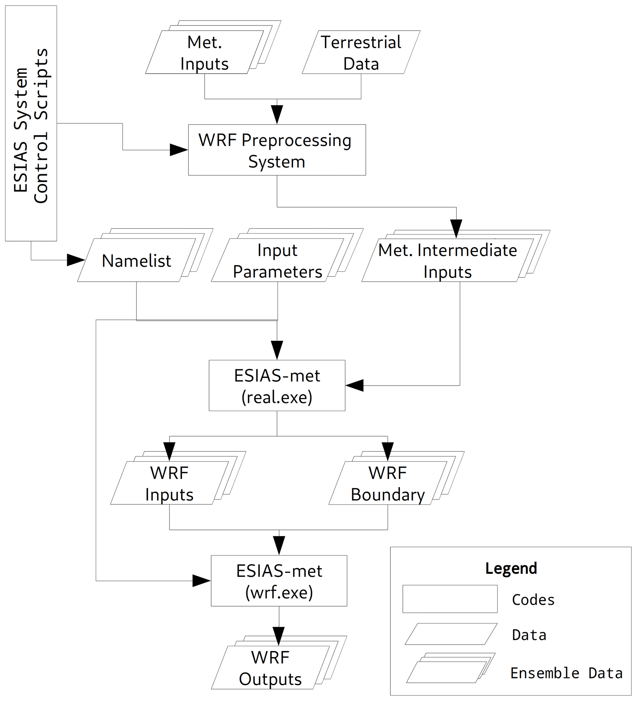
Figure 1 The concept of ESIAS-met scheme and the whole process of ESIAS-met. The ESIAS system control scripts control the WRF processing system and the namelist to generate necessary inputs.

The ESIAS-met executables apply the MPI for large-ensemble simulations with interactive members on high-performance computers (HPCs; large individual ensemble simulations on HPCs are inhibitive and cause long queuing times). The main purpose of ESIAS-met is to perform large-ensemble simulations with stochastic schemes, and thus, both the stochastically perturbed parameterization tendency (SPPT; Buizza et al., 1999) and the stochastic kinetic energy backscatter scheme (SKEBS; Berner et al., 2009, 2011) are implemented.

2.2 Model setup

ESIAS-met is driven with boundary conditions and intermediate meteorological inputs from GEFS and with MODIS (Moderate Resolution Imaging Spectroradiometer) land use data. The map projection is Lambert conformal, with a central point (54^∘ N, 8.5^∘ W). The horizontal resolution is 20 km and the number of horizontal grid points is 180×180. There are 50 vertical layers, only the first 11 of which have uneven spacing through the vertical direction, especially near the surface. In this study, we do not use any finer, nested domain due to the computational demand. We thus evaluate 10 microphysics which are limited to no cloud-resolving simulations (UCAR, 2015). A previous study and large sensitivity analysis by Stergiou et al. (2017) tested 68 different physics configurations also on the European domain, though with a different approach, thereby changing the physics options one at a time.

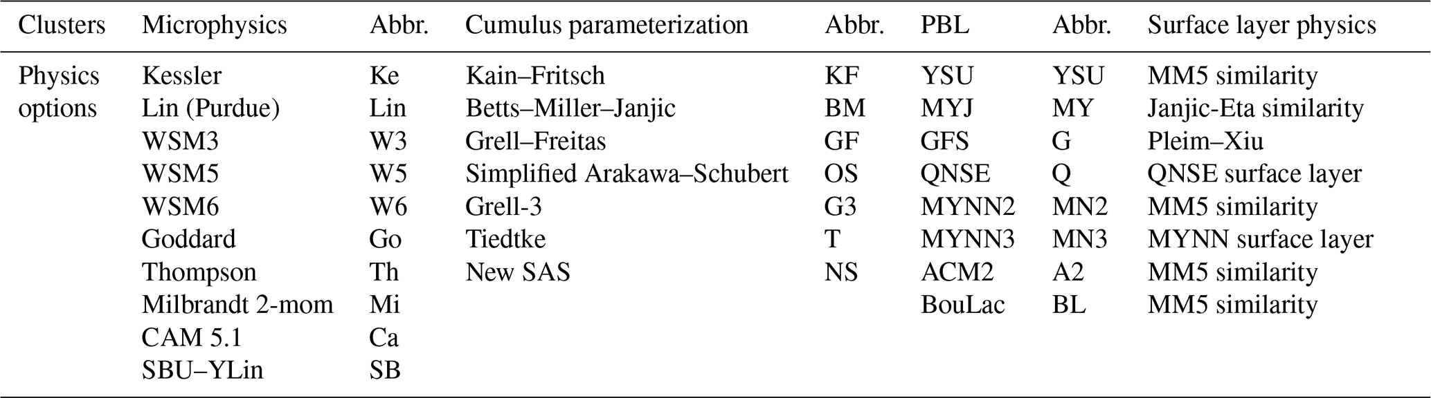
Large-ensemble simulations with members of different physics were created in three sets to iteratively investigate the optimal configuration for cloud cover and the photovoltaics forecasting application. The first set (Set 1) is the broadest, with 560 combinations of microphysics, cumulus parameterization, and planetary boundary layer physics. Accordingly, only a few test cases with differing but typical cloud conditions could be afforded for Sets 1–3, whereas both the seasonality and probabilistic performance were tested for the final four configurations in Set 4. The Set 1 combinations and the acronyms for the WRF physics and parameterizations are listed in Table 1. We note that the official documentation recommends setting the surface layer physics with specific planetary boundary layer physics in WRF (UCAR, 2015). Five-layer thermal diffusion is employed for land surface physics, Dudhia for shortwave radiation physics, and the Rapid Radiative Transfer Model (RRTM) for longwave radiation physics in this set of numerical experiments.

Table 1 Employed physics configuration of Set 1, which summarized $\mathrm{10}\times \mathrm{7}\times \mathrm{8}$ configurations. The abbreviation is followed by the physics name. The PBL is used with certain surface layer physics indicated in the same row of PBL option.

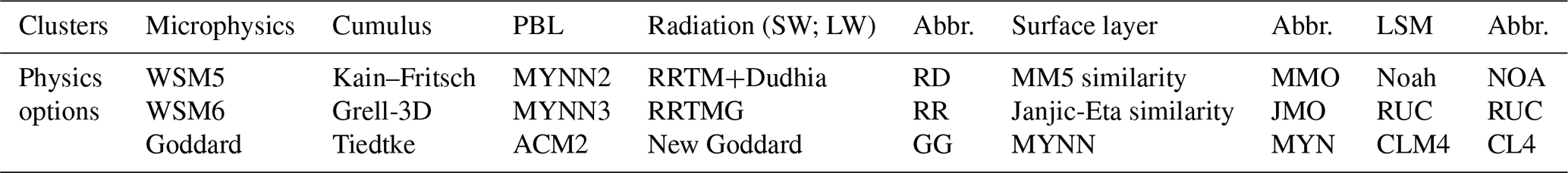
Set 2 takes a sub-selection from the Set 1 results and adds land surface models, shortwave radiation schemes, and longwave radiation schemes to form the additional 513 combinations described in Table 2. We note here that the PBL ACM2 only considers the surface layer physics of MM5 similarity and thus does not apply to the other surface layer physics models. The land surface model CLM4 also does not employ Eta similarity and thus we exclude this combination. For the long- and short-wave radiation physics, we have only three combinations, i.e., RRTM and Dudhia, RRTMG (Rapid Radiative Transfer Model for GCMs) and RRTMG, and Goddard and Goddard for the short- and longwave radiation physics schemes, respectively. For surface layer physics, we employ Monin–Obukhov (MO) similarity and hence the revised MM5 MO similarity (listed as MM5 similarity) and Janjic-Eta MO similarity are utilized. The MYNN surface layer scheme is used to investigate its suitability with the MYNN2 and MYNN3 PBL physics. The sophisticated land surface models (LSMs) of CLM (Community Land Model version 4) and Noah LSM are tested along with Rapid Update Cycle (RUC) LSM, which performs similarly to the other two LSMs (Jin et al., 2010).

Table 2 Employed physics configuration of Set 2, which summarized $\mathrm{3}\times \mathrm{3}\times \mathrm{3}\times \mathrm{19}$ configurations. Both revised MM5 MO (MMO) and Janjic-Eta MO (JMO) similarity is based on Monin–Obukhov similarity, and therefore, we use MO to represent the abbreviation.

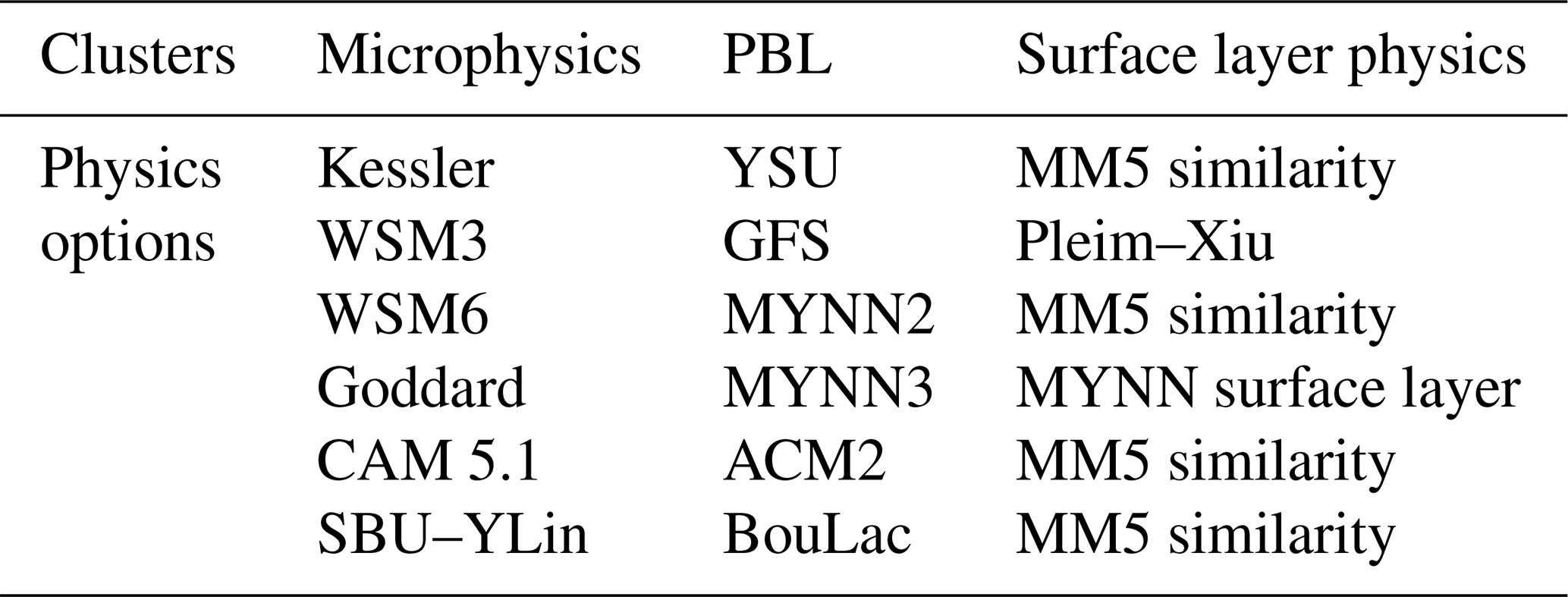
Following the Set 2 results, six microphysics and six combinations of PBL and surface layer physics were chosen for 36 further combinations for stochastic study in Set 3 (listed in Table 3). Here, 32-member ensembles were created with SKEBS for a total of 1152 members. All Set 3 simulations employ the Grell-3 cumulus parameterization, the Dudhia shortwave radiation physics, the RRTM longwave radiation physics, and the RUC LSM for land surface physics. Although ESIAS-met can employ both SPPT and SKEBS schemes, we only apply SKEBS in this experiment. According to Jankov et al. (2017) and Li et al. (2019), SKEBS can produce a large-ensemble spread. Berndt (2018) also reports that SKEBS can more effectively produce instability in ESIAS-met than SPPT. We therefore use it to study the extent of the spread that one single stochastic scheme can produce. One ensemble member of the 32 is not perturbed as to double as a control run.

Table 3 Employed physics configuration of Set 3, which summarizes 6×6 configurations. The PBL is used with certain surface layer physics indicated in the same row of PBL option.

Finally, four combinations were selected for long-term simulations as part of a project concerning energy predictions and quantile calibrations (Dupuy et al., 2021). These data include day-ahead predictions for every other day in 2018, and we use it here against a half-year of available satellite data to verify the reliability of the recommendations under more diverse conditions than the limited test cases. The set of four combinations in Table 4 are WSM6-MYNN2, WSM6-MYNN4, Goddard-MYNN2, and Goddard-MYNN3. The cumulus parameterization and surface physics are Grell-3D and revised MM5 MO similarity, respectively. The RUC LSM is used for land surface physics. These simulations were conducted over the same European domain but with 15 km resolution and using ECMWF instead of GEFS as input due to the availability of the data. The model grid cells increase from 180×180 to 220×220 in horizon.

Table 4 Four select physics configurations of Set 4 ($\mathrm{2}\times \mathrm{2}\times \mathrm{1}$).

2.3 Model performance evaluation and measurements

2.3.1 Ternary cloud mask

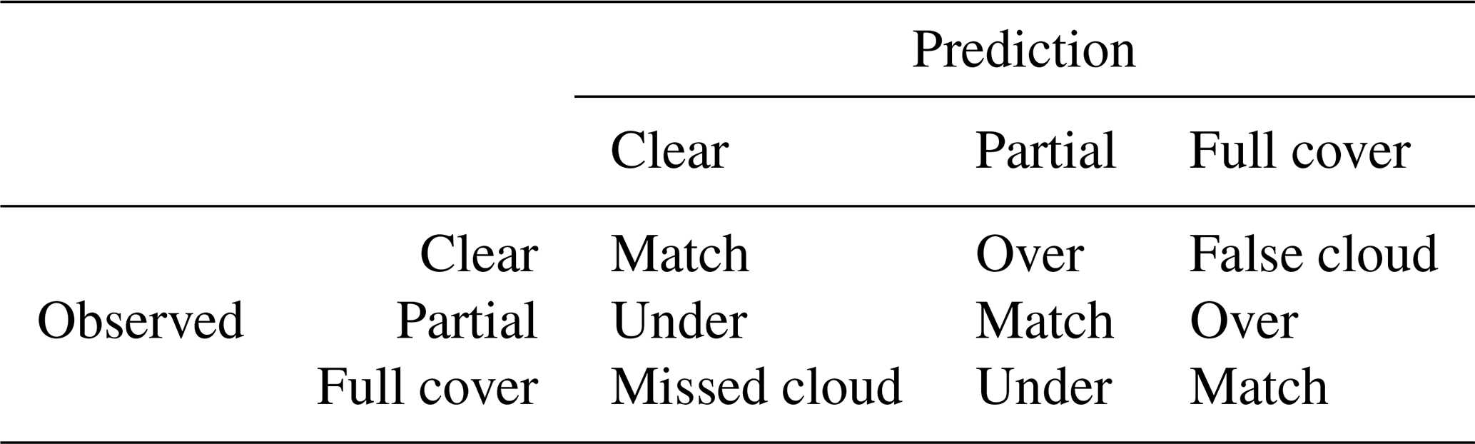
To determine the accuracy of the cloud cover prediction, we apply the determination method and separate the cloud cover fraction in each grid cell into three gradations, namely clear-sky (<5 %), partially cloudy (≥5 % and <95 %), and fully cloudy (≥95 %), to show more detail beyond a binary cloud mask. The definition of clear sky follows the definition from Automated Surface Observing System (ASOS; Diaz et al., 2014), with 5 % cloud fraction, while the full cover is defined analogously at 95 % cloud fraction. The inclusion of partial clouds adds detail to the comparison of the simulation and satellite data, which of course decreases agreement rates relative to a binary mask. Table 5 illustrates the ternary detection possibilities for deterministic simulations. The traditional binary detection classifies the outcome into just three categories, namely false (overprediction), miss, and match. Ternary determination increases this to five categories by including partially cloudy areas and the prediction ability for the different physics configurations. Here, we use the convention that “under” and “over” represent the partial matches between fully missed or false clouds.

Table 5 The five possible outcomes for the detection of predicted cloud cover compared to observation, where 0 %–5 %, 5 %–95 %, and 95 %–100 % are defined as clear, partial, and full cover, respectively. In addition to the classifications of match, miss, false/overprediction in the detection method for binary condition, we have partial matches of “under” and “over”.

2.3.2 Kappa score

The Kappa (κ) score is used to measure agreement between two or more raters, using determination in large datasets (like for subjects in psychological research; Fleiss and Cohen, 1973). This score for deterministic results is used widely in natural sciences such as land science for determining the change of land use (e.g., Schneider and Gil Pontius, 2001; Yuan et al., 2005; Liu et al., 2017) or machine learning for scoring and validation (e.g., Dixon and Candade, 2008; Islam et al., 2018). The equation of the Kappa score for multiple raters is calculated as follows:

$$\begin{array}{}\text{(1)}& {\displaystyle }\mathit{\kappa }={\displaystyle \frac{\overline{P}-{\overline{P}}_e}{\mathrm{1}-{\overline{P}}_e}}\text{(2)}& {\displaystyle }\overline{P}={\displaystyle \frac{\mathrm{1}}{N\cdot n(n-\mathrm{1})}}\sum _{i=\mathrm{1}}^N\sum _{j=\mathrm{1}}^k{n_{ij}}^{\mathrm{2}}-Nn\text{(3)}& {\displaystyle }{\overline{P}}_e={\displaystyle \frac{\mathrm{1}}{(N\cdot n{)}^{\mathrm{2}}}}\sum _{j=\mathrm{1}}^k\sum _{i=\mathrm{1}}^N{n_{ij}}^{\mathrm{2}}.\end{array}$$

$\overline{P}-{\overline{P}}_e$ is the actual degree of agreement between raters, and $\mathrm{1}-{\overline{P}}_e$ is the degree of agreement when matching correctly. For a number of n raters, N subjects will be rated into k categories. Each n_ij represents the number of raters agreeing on the jth category. In our work, the five possible outcomes in Table 5 are the categories for the two raters, which are the simulation and observation results for the grid cells as subjects.

κ has a maximum value of 1 and can also be negative. The maximum κ means a full match between the two datasets. κ between 0 and 1 indicates a partial match between the two datasets, while negative κ indicates some anti-correlation in the matching (Pontius, 2000). A good model result should result in positive κ.

2.3.3 Kernel density estimation

Kernel density estimation (KDE) is a method to approximate the probability density function of dataset. A variable X with n independent data points x₁, x₂, …, x_n at x can be expressed as follows:

$$\begin{array}{}\text{(4)}& f_h\left(x\right)={\displaystyle \frac{\mathrm{1}}{nh}}\sum _{i=\mathrm{1}}^{n}K\left({\displaystyle \frac{x_i-x}{h}}\right),\end{array}$$

where h and K are the bandwidth and kernel functions, respectively. The kernel function K(u) can be uniform $\left(\right(\frac{\mathrm{1}}{\mathrm{2}}\left)I\right(\left|u\right|\le \mathrm{1}\left)\right)$ or Gaussian $\left(\frac{\mathrm{1}}{\sqrt{\mathrm{2}\mathit{\pi }}}\exp \right((-\frac{\mathrm{1}}{\mathrm{2}})u^{\mathrm{2}}\left)\right)$, depending on the purpose. This study uses the Gaussian kernel. Here we also propose normalizing the KDE with the cumulative KDE with x in the range from 1 to m as follows:

$$\begin{array}{}\text{(5)}& f_{h,\text{acc}}\left(i\right)=\sum _{j<i}{f}_h\left(x_j\right),\text{ for }i=\mathrm{1},\mathrm{2},\mathrm{\dots },m.\end{array}$$

The resulting cumulative KDE can be normalized by the last item of f_h,acc(i), i.e., f_h,acc(x_m), and therefore a normalized cumulative KDE can be used to show the cumulative probability distribution of the data, which increases monotonically.

3 Data description

3.1 Input data

The initial and lateral boundary conditions are generated from the control data of the GEFS of the National Centers for Environmental Prediction (NCEP; Hamill et al., 2013). This dataset has approximately 40 km resolution and 42 vertical levels. The detail on the GEFS data is described by Hamill et al. (2011). To better represent the forecasting skill from April to September in 2015, we conduct 48 h simulations beginning on 13 April, 15 May, 17 June, 19 July, 23 August, and 21 September. These are more or less random days in different months without rare conditions, as we target the general forecasting performance for PV. Due to limited computational resources, we are only able to demonstrate Sets 1, 2, and 3 in ESIAS-met for day-ahead simulations beginning on these 6 random days. Each simulation uses inputs from the GEFS reforecast data with a 3 h resolution. The soil texture and land use condition are based on MODIS and the Noah-modified 20-category International Geosphere Biosphere Programme (IGBP)-MODIS land use data with 2 min and 30 s resolutions, respectively. The target domain covers most of Europe, with a 20 km horizontal resolution. Figure 2 shows the whole area of the target domain and the elevation height. The ECMWF-reanalyzed ERA5 data are also used as initial conditions in 2018 for a yearly day-ahead weather forecasting simulation. We apply the 3 h input and lateral boundary conditions as inputs for ESIAS-met.

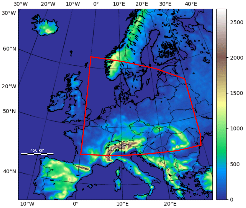
Figure 2 The topography of the target domain, the European domain, for the simulation. The red line indicates the area for validating the result with cloud cover from the satellite.

3.2 Satellite data

To validate and rate the model performance, we use the cloud fraction cover (CFC) product from the EUMETSAT Climate Monitoring Satellite Application Facility (CM SAF; Stengel et al., 2014). The data are corrected and generated from the Spinning Enhanced Visible and InfraRed Imager (SEVIRI) on Meteosat-8, which uses the visible, near-infrared, and infrared wavelengths to retrieve cloud information. The hourly CFC data have level 2 validation (Stöckli et al., 2017) for the accuracy of total synoptic cloud cover, and the data are corrected by the algorithm from Stöckli et al. (2019), using the clear-sky background and diurnal cycle models for brightness temperature and reflectance. The calculation of CFC employs a Bayesian classifier. This product covers the spatial domain of Europe and Africa back to 2015, although this product was discontinued after March 2018. The data are cropped to the central European model domain. Since the CFC data do not include the northern part of Europe and have limitations at high viewing angles above the 60th parallel (Stöckli et al., 2017), we exclude this part of the domain in the analysis.

The satellite data are provided on a regular grid with a $\mathrm{0.05}{}^{\circ }\times \mathrm{0.05}{}^{\circ }$ horizontal resolution, which is finer than the simulation setup of 20 km×20 km, equivalent to 0.31^∘ longitude and 0.18^∘ latitude at the model domain center. In order to compare the satellite data to the lower-resolution model results, we simply average the CFC pixels within each grid cell (other studies, like Bentley et al., 1977, may use all points within a fixed radius, which may or may not overlap). The target value for any model grid point is then averaged over 12 to 36 observation points, depending on the location.

The viewing zenith angle of the satellite of course creates some uncertainty in the actual observation locations due to cloud heights. This mostly vertical shift can be up to a few pixels for high clouds within the EUMETSAT grid itself; however, it is at most one 20 km model point in uncertainty, such that this has only a small effect on the discrete cloud mask of the aggregated value and is negligible for the κ scores, when considering the actual resolution of cloud details arising out of the model. Should higher-resolution simulations be investigated in the future, however, this will have to be taken into account using, e.g., a satellite simulator on the model data.

Figure 3 shows the cumulative domain cloud cover over time for each test day in 2015 according to the observation. The blue and orange curves represent the cloud cover during daytime, while the red and cyan curves represent the cloud cover at night. For the cumulative plots of KDE, which is normalized to 1.0, curves with a higher accumulative rate (rapid growth on the y axis) represent high clear-sky rates in the data. Curves with a lower accumulative rate (y axis) represent more full cloud cover. The 17 June and 23 August cases exhibit a very high variation over the 48 h of simulation time. Moreover, 17 June shows a higher cloud cover than 23 August. The 13 April, 15 May, 19 July, and 21 September cases are similar in the cloud cover condition, since the cumulative distributions show that the variation in cloud cover is smaller than for 17 June and 23 August. However, both the 13 April and 19 July cases show a higher cloud cover in the early morning and in the early evening than for the 15 May and 21 September cases, respectively. In general, the 23 August and 21 September cases can represent the cloud cover condition with high variability and low variability, respectively.

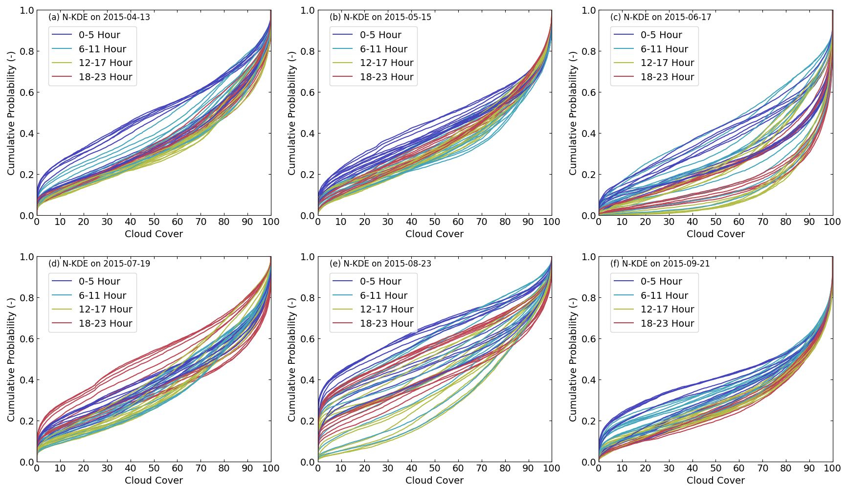
Figure 3 The cumulative KDE of cloud cover for the six simulation cases in UTC time. The colors distinguish the different cloud cover. The different colors represent different time periods in a day, as shown in the legend.

Finally, for the year-long simulation we used EUMETSAT cloud mask data that were available for comparison to the simulation results. This binary cloud mask is also an operational product from SEVIRI that covers the full disk and distinguishes cloudy and cloud-free pixels, as derived by the Meteorological Product Extraction Facility.

4 Results

4.1 Simulation efficiency

The simulations were performed on the JUWELS (Jülich Supercomputing Centre, 2019) high-performance computer utilizing Intel Xeon 24-core Skylake CPUs (central processing units; 48 cores per node) and 96 GB of main memory. We use 12 CPUs per ensemble member, meaning 6720 total CPUs for 560 ensemble members and 6156 CPUs for 513 ensemble members to perform the large-ensemble simulation for Sets 1 and 2. These large-ensemble simulations are completed by JUWELS without performing farming on the HPCs, with the stability of the large simulations guaranteed by ESIAS.

Different physics configurations not only affect the resulting weather data but also significantly impact the computation time. Figures 4 and 5 show the average time consumption (solid line) and the range of the time consumptions (color fill) for the configurations of microphysics and planetary boundary layer physics, respectively. We use the simulation case on 21 September as an example. The most time-consuming simulations always include CAM5.1 (average of 26 095 s) microphysics, and the quickest have Kessler (average of 10 404 s), which only parameterizes the autoconvection, precipitation clouds, the evaporation of precipitation, and the condensation–evaporation function in the continuity equation. For the simulation of planetary boundary layer physics, the slowest configuration is QNSE (quasi-normal-scale elimination; average of 16 967 s), and the fastest is GFS (NCEP Global Forecast System; average of 12 440 s). The cumulus parameterization has the smallest effect on time consumption, with the most time-consuming being Grell-3 (average of 14 715 s), and the least time-consuming being Betts–Miller–Janjic (average of 13 447 s), where the difference is only 9.4 %.

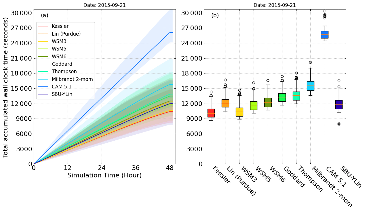
Figure 4 The (a) total accumulated simulation time. (b) A box plot of different microphysics configurations within each simulation hour on 21 September 2015. The upper and lower boundaries of the color fill indicate the maximum and minimum simulation time with other physics configurations.

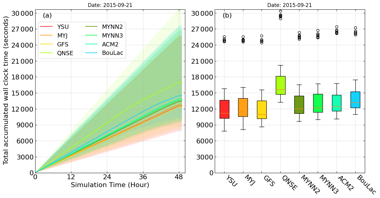
Figure 5 The (a) total accumulated simulation time. (b) A box plot of different PBL configurations within each simulation hour on 21 September 2015. The upper and lower boundaries of the color fill indicate the maximum and minimum simulation time with other physics configurations.

The differences between the first and third quartiles show how much the different physics configurations affect the simulation speed, as shown in Figs. 4b and 5b. For the physics clusters of microphysics, PBL physics, and cumulus parameterization, the average quartile difference is near 1500, 3500, and 3700 s, respectively. The outliers involve CAM5.1 microphysics, which is the most computationally expensive. The most time-consuming part is the configuration of the microphysics. The average time consumption is similar for the clusters of PBL physics and of cumulus parameterization, except for the QNSE PBL physics, which consumes 5000 s more simulation time than other PBL physics. The box plot confirms that CAM5.1 microphysics and QNSE PBL physics are the most time-consuming.

4.2 Set 1 sensitivity analysis: clusters of microphysics, PBL, and cumulus parameterization

The simulation results used for comparison with the satellite data exclude the first 12 h, as the model is run in weather forecasting mode and hence can take 6–12 h to converge (Jankov et al., 2007; Kleczek et al., 2014). Only the last 36 h of the simulation output are therefore used to compare with the satellite data.

The 560 simulations were performed with the target dates and times from Sect. 3.1. The heat maps in Figs. 6 and 7 represent two different test case results with high and low variabilities, based on the cloud cover, respectively. Both figures indicate that the κ scores of the microphysics cluster by their cumulus parameterization and PBL physics. The cloud mask results indicate that the CAM5.1 cluster not only outperformed the cloud cover prediction of the other microphysics but also that Goddard and WMS3 performed well. The κ indicates that the Kessler microphysics predicted the worst cloud cover overall, irrespective of the PBL physics or cumulus parameterization used. The combination of the three cumulus parameterizations, Grell–Freitas, Grell-3, and New SAS (Simplified Arakawa–Schubert), and the PBL physics GFS diminishes the prediction of the cloud cover. The results from the other four cases can be found in Figs. S1–S4 in the Supplement.

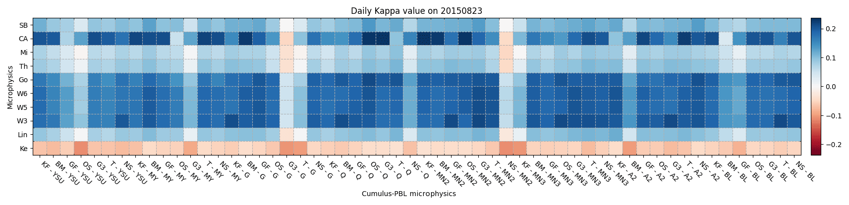
Figure 6 The heat map of the average κ for every configuration for the clusters of microphysics (y axis) with the cluster of cumulus parameterization and PBL (x axis) for the simulation case on 23 August for Set 1. The data only use the last 36 h of simulations for calculating κ.

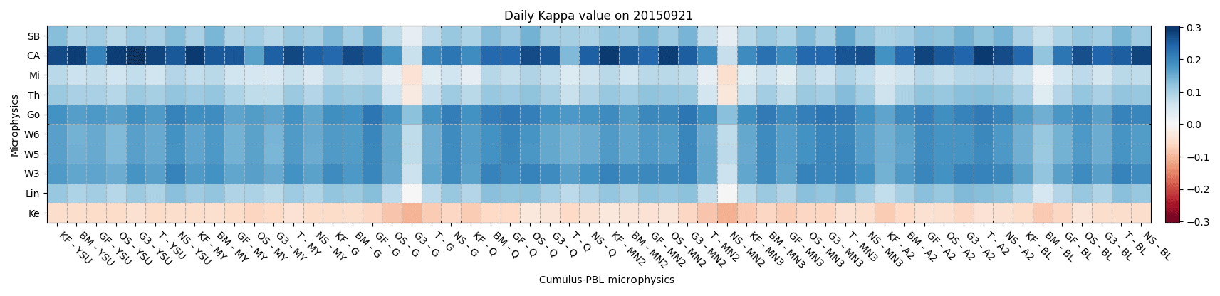
Figure 7 The heat map of average κ for every configuration for the clusters of microphysics (y axis) with the cluster of cumulus parameterization and PBL (x axis) for the simulation case on 21 September for Set 1. The data only use the last 36 h of simulations for calculating κ.

The overall results for κ from the six test cases (Fig. 8a) confirm that CAM5.1 performed best for cloud cover and that both the WRF single moments 3 (WSM3) and the Goddard microphysics also performed well. The only exception is the 13 April case, where the Goddard microphysics cluster outperformed the other microphysics. The simulations for the 15 June and 23 August cases were performed well by the Goddard microphysics and the WMS3, WSM5, and WSM6 microphysics clusters. Here, the cloud cover varies more than in the other cases. The performance of the Goddard microphysics and the WMS3, WSM5, and WSM6 microphysics clusters was equal to the CAM5.1 microphysics cluster in the cases with large cloud cover variation, as for 17 June and 23 August.

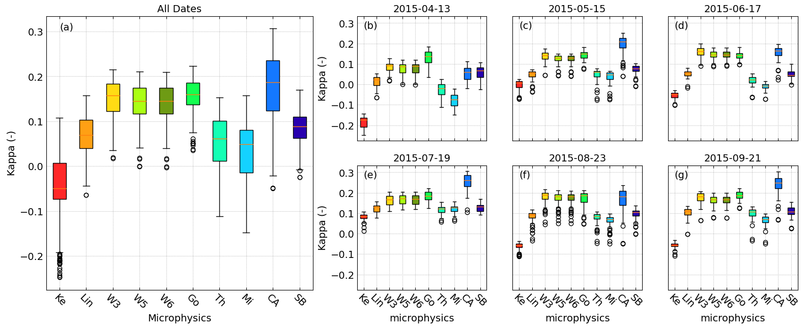
Figure 8 The box plots of κ in panel (a) show all the simulation dates and those on (b) 13 April, (c) 15 May, (d) 17 June, (e) 19 July, (f) 23 August, and (g) 21 September for Set 1.

Figures 9 and 10 show the average cloud fraction from hours 12 to 48 from both the satellite data and the simulation result for 23 August and 21 September, respectively. In this simulation case, we use the different microphysics and the cumulus parameterization of Grell-3D and the PBL physics of MYNN3. In the 23 August case, the sky is partially clear above the North Sea and in Eastern Europe and rather cloudy around the Alps. From the selected microphysics, Kessler, WSM6, Goddard, CAM5.1, and SBU–YLin (Stony Brook University Y. Lin), different cloud fraction conditions are shown. WSM6, Goddard, and SBU–YLin provided a good simulation of the clear sky above the North Sea and Eastern Europe, while the sky above the Alps is as cloudy, as in the satellite data. The worst case, Kessler, shows a large cloud cover condition over Eastern Europe, which contradicts the observation during the dynamic 23 August case.

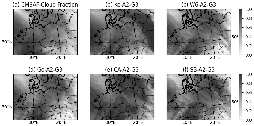
Figure 9 Average cloud cover fraction for 36 h of (a) satellite data and simulation by different microphysics, including (b) Kessler, (c) WSM6, (d) Goddard (e) CAM5.1, and (f) SBU–YLin. All simulations are configured with Grell-3D and ACM2 PBL physics, which performed a more skilled prediction than any other combination from 23 August.

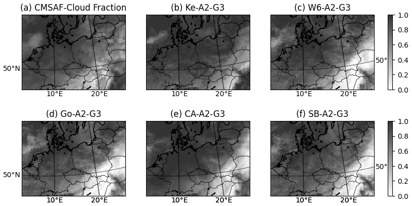
Figure 10 Average cloud cover fraction for 36 h of (a) satellite data and simulation by different microphysics, including (b) Kessler, (c) WSM6, (d) Goddard (e) CAM5.1, and (f) SBU–YLin. All the simulations are configured with Grell-3D and ACM2 PBL physics, which performed a more skilled prediction than any other combination from 21 September.

The 21 September case is a cloudy day with low variability in cloud cover. A band of clear sky occurs above Austria, Slovakia, southern Poland, and Ukraine (Fig. 10). The WSM6 and Goddard microphysics simulated less cloud over the clear-sky band but produced less cloud cover overall within the model domain. Kessler simulated a cloudy condition over central Europe.

In Fig. 11, the KDE of the cloud cover shows the probabilistic distribution of the average cloud cover for the 36 h of simulation after hour 12 for the 23 August and 21 September cases. For 23 August, CAM5.1 microphysics worked well for the κ score but overestimates the cloud cover. The overestimation of cloud cover causes CAM5.1 to perform worse than in the 15 May, 19 July, and 21 September cases. WSM3, WSM5, WSM6, and Goddard microphysics show similar trends of cloud cover distribution, as in the satellite image. For the 21 September case, the clear-sky condition (<5 % of cloud cover) is captured well by CAM5.1, but the cloud cover distributions of the entire CAM5.1 cluster differ from that in the satellite image.

Figure 11 The probabilistic function from the kernel density estimation (KDE) of the average cloud fraction for the last 36 h simulation for (a) case 23 August and (b) case 21 September. The PBL physics is by ACM2 and the cumulus parameterization is by Grell-3D. The solid color lines depict the KDE from the simulations, and the black dashed line is the KDE from the satellite data.

By comparing the result with the microphysics cluster, PBL physics cluster, and cumulus parameterization cluster, we can conclude that there is good performance for cloud simulation by CAM5.1, WSM3, and Goddard microphysics. The PBL physics and cumulus parameterizations have fewer impacts on the simulation of cloud cover than the microphysics. To obtain a comprehensive result on cloud cover, we investigate the impact of using different microphysics on the average cloud cover distributions. However, the temporally and spatially averaged cloud covers provide less information and less variability over time. To determine the simulation skill on the spatial patterns, we score the simulation result by calculating the κ score using the pixels in the simulation domain.

4.3 Set 2 sensitivity analysis: clusters of microphysics, PBL, cumulus, radiation schemes, surface layer physics, and land surface parameterization

Additional components to the physics configuration include different longwave and shortwave radiation physics and land surface layer physics. However, there are more than a million possible combinations of all physics options. We therefore narrow down the choice of the microphysics, PBL physics, and cumulus parameterization from Sect. 4.2. Accounting for the treatment of the graupel mixing ratio for ESIAS-chem, we predominantly use the microphysics of WSM5, WSM6, and Goddard. CAM5.1 performed the best across five of the six test cases, but it is not included because of the higher computational cost. MYNN2, MYNN3, and ACM2 (Asymmetrical Convective Model version 2) are selected because of their good performance with the selected microphysics. From the heat map (Fig. 6), both Grell 3D and Tiedtke work well with Goddard and WSM6. We also choose Kain–Fritsch, which is widely used (e.g., Warrach-Sagi et al., 2013; Knist et al., 2017), for comparison. The PBL physics from MYNN2, MYNN3, and ACM2 performed well across all the simulations and is chosen for this simulation case.

Figure 12 shows the heat map of the 21 September simulation case and the physics configuration of Goddard and ACM2. The Goddard radiation schemes perform skillful predictions of cloud cover. This heat map also indicates good combinations of microphysics, cumulus parameterization, and radiation schemes, as well as combinations of PBL physics, surface physics, and land surface models by row and column, respectively. By row, the Goddard works better with the Tiedtke and Grell-3D cumulus parameterization overall. By column, the heat map shows that ACM2 PBL physics can improve the simulation with all the microphysics but with less improvement for the radiation schemes RRTM and Dudhia. Under the same condition, MYNN3 with Grell-3D and RRTM and Dudhia perform better with WSM5, WSM6, and Goddard microphysics. From the 513 combinations of physics configurations, the range of the κ score is between 0.15 and 0.24. The microphysics and the PBL physics are chosen from the results of Sect. 4.2, which is why the improvement is not significant compared to the improvement from changing either the longwave and shortwave radiation scheme or the surface layer physics or land surface models.

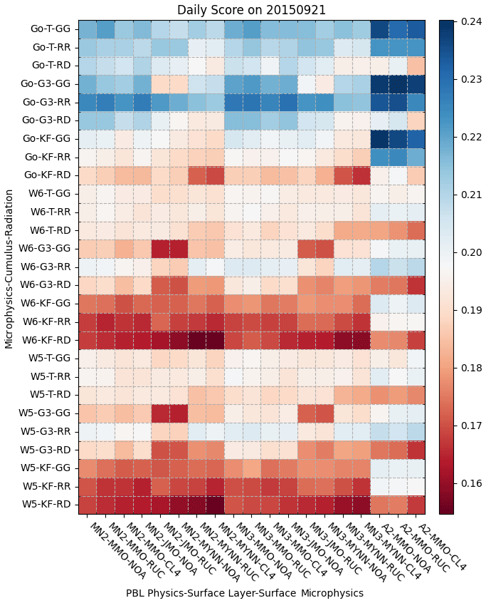
Figure 12 The heat map of the average κ for the configuration for the clusters of microphysics, cumulus parameterization, and the radiation physics (y axis) with the cluster of PBL physics, surface physics, and the land surface model (x axis) for the simulation case on 21 September for Set 2. The data only use the last 36 h of simulations for calculating κ.

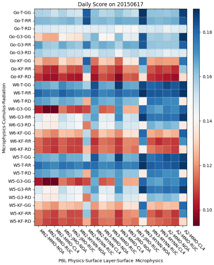
Figure 13 The heat map of the average κ for the configuration for the clusters of microphysics, cumulus parameterization, and the radiation physics (y axis) with the cluster of PBL physics, surface physics, and the land surface model (x axis) for the simulation case on 17 June for Set 2. The data only use the last 36 h of simulations for calculating κ.

In the 17 June case (Fig. 13), the cloud cover distribution has a very high variability, and therefore, the simulation skills increase their variabilities in κ with different combinations. When all microphysics clusters have a Kain–Fritsch score less than 0.1, then the simulations are better with the combinations of MYNN2/MYNN/RUC, MYNN3/MYNN/Noah, and ACM2/MMO/CLM4. The pattern of outperforming κ is also shown in the result for 19 July (Fig. S7), which includes the worst κ score among the six cases. The results from the other four cases can be found in Figs. S5–S8.

The box plot (Fig. 14) shows the overview of the six cases along with the clusters of microphysics and cumulus parameterization, which show less variability and are very similar for each case, indicating that high variability occurs from other physics clusters. The whiskers of the box plot (as maximum or minimum of the data or $\text{third quartile}\pm \mathrm{1.5}\times \text{interquartile range}$) show that combinations with the Grell-3D cumulus parameterization can achieve the maximum average κ scores. The Goddard microphysics and Tiedtke cumulus parameterization can be the least variable, and their median κ indicates that this combination can outperform other microphysics and cumulus parameterization clusters. The box plots from all the cases show that the cumulus parameterizations of Grell-3D and Tiedtke, which are more advanced than Kain–Fritsch, can improve the score. The resulting κ does not significantly differ between Grell-3D and Tiedtke.

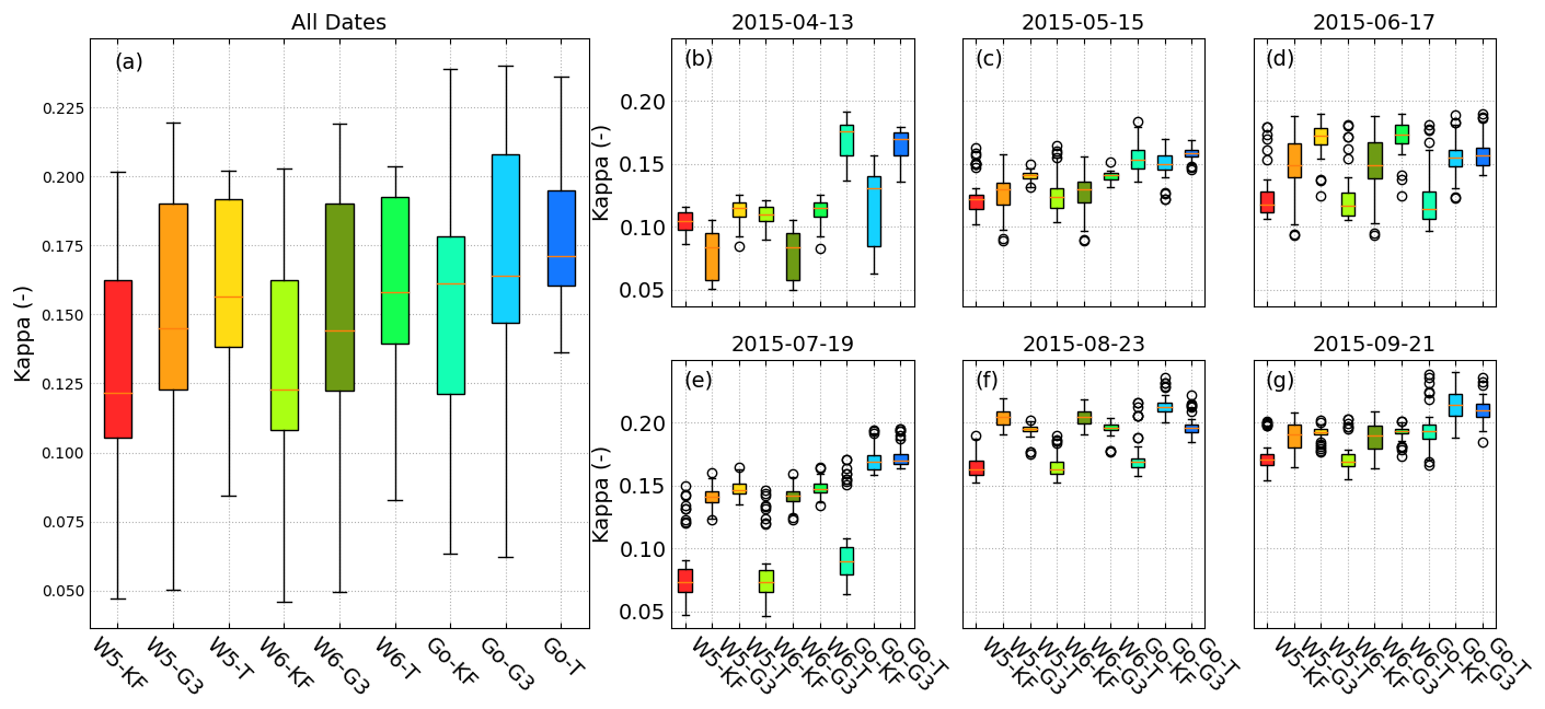
Figure 14 The box plots of κ from microphysics and cumulus parameterization clusters in panel (a) show all the simulation dates and those on (b) 13 April, (c) 15 May, (d) 17 June, (e) 19 July, (f) 23 August, and (g) 21 September for Set 2.

4.4 Set 3 sensitivity analysis: impact of microphysics and PBL on stochastic simulation

Stochastic weather forecasting requires many diverse simulation ensemble members. To study the impact of the physics configuration on the stochastic simulation, we generated 31+1 ensemble members in 48 h ensemble runs. The total cloud fractions again after 12 simulation hours are used to analyze the differences from the model configuration and their impact on probabilities. The stochastic experiments are simulated for the same cases and domain and with the same input data as before.

Figure 15 shows the probabilistic cloud cover fraction within the 25th–75th percentiles and 5th–95th percentiles of the simulations. The development of the mean cloud cover fraction is compared to the mean cloud cover fraction of the satellite data. The rmse (root mean square error) and standard deviation are used to show the comprehensive result of the temporal cloud cover development within the final 36 h of the simulations.

Figure 15 The mean cloud cover fraction (–) and the observation from the satellite (black line) and by simulation (color line) from the combination of microphysics (by different colors) and PBL physics (in different rows) for the case on 23 August. The color block represents the range of percentiles, the darker block is limited between 25 % and 75 %, and the lighter block is limited between 5 % and 95 %. The gray block indicates the spin-up time for ESIAS-met, which is not included in the root mean square error (rmse), standard deviation ($\overline{\mathit{\sigma }}$), or the mean simulated cloud cover fraction ($\overline{x}$).

The Kessler microphysics appeared to overestimate the cloud cover fraction and have the largest rmse of all microphysics. Moreover, the two peaks in the cloud cover fraction around the hours of 12 and 36 of the simulation are not clearly captured by the Kessler ensemble, though this is better than in most cases in the combination with ACM2. The SBU–YLin microphysics and ACM2 PBL physics achieved the smallest rmse, and the WSM6 microphysics and ACM2 PBL physics were second best. The biggest standard deviation and therefore ensemble spread was produced by the SBU–YLin and MYNN2 PBL physics. In the 21 September case (Fig. S13), the WSM6 microphysics showed the greatest spread and largest standard deviation. In both cases, the CAM5.1 microphysics combined with the GFS PBL physics to produce the narrowest probability distribution of the cloud cover fraction. The color blocks show the simulation skill in capturing the cloud cover fraction within a certain percentile. The MYNN2, MYNN3, and ACM2 PBL physics not only produce a larger probabilistic distribution than the other PBL physics but also perform better with the WSM6, Goddard, and SBU–YLin microphysics. The results from the other four test cases can be found in Figs. S9–S12.

Figure 16 summarizes the rmse performance of the ensemble mean against the observed domain total cloud fraction. Figure 17 illustrates the time-averaged ensemble spread with the standard deviation (SD) of the domain total cloud fraction. From the rmse, SBU–YLin had the best mean total cloud fraction over all six cases, with a more variable cloud fraction according to the SD. The WSM3, WSM6, Goddard, and SBU–YLin with MYNN3 and ACM2 produced more accurate average cloud fractions than the other combinations. Overall, the WSM series and SBU–YLin better represented the uncertainty than the other microphysics, while MYNN3 and ACM2 improved the simulation accuracy.

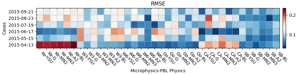
Figure 16 Heat map of the RMSE between the ensemble mean total cloud fraction and observation, averaged over the last 36 h of the simulations, shown for each cluster of microphysics and PBL physics (columns) for all test cases (rows). In the color scale, red represents higher RMSE and poorer performance.

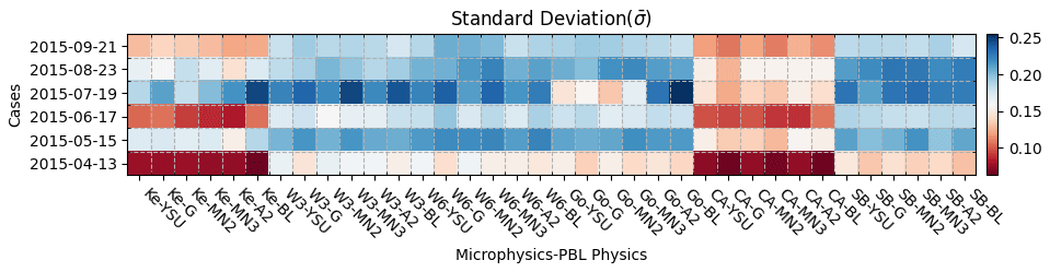
Figure 17 Heat map of the ensemble standard deviation ($\overline{\mathit{\sigma }}$) of the mean total cloud fraction, averaged over the last 36 h of the simulations, shown for each cluster of microphysics and PBL physics (columns) for all test cases (rows). In this heat map, blue indicates larger $\overline{\mathit{\sigma }}$ and greater ensemble spread.

4.5 Set 4 sensitivity analysis: long-term validation

Sets 1–3 address over a thousand model combinations. Ideally, all combinations could be tested over a full year to capture diverse conditions and seasonality and to benchmark their operational performance. The aggregate computational expense of all combinations is unfortunately too great for this. For the four most promising models listed in Table 4, however, ESIAS could be economically tested over a full year and these four cases compared to roughly 6 months of available satellite data in 2018 by calculating the κ with the cloud mask data. A summary of these results is shown in Fig. 18.

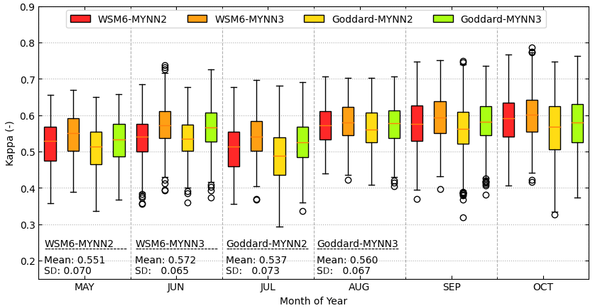
Figure 18 The monthly box plot of the four cases by the κ for the 6 months simulation from June to October. The yearly means and standard deviations of the κ are shown for four cases at the bottom of the plot.

In this test of the more generalized model performance, the models scored similarly, with the WSM6 microphysics having higher κ and slightly lower standard deviations than Goddard with the same PBL, and likewise, MYNN3 performed better than MYNN2 for the same microphysics. In the plot, the maximum κ values are thus generally reached by points with MYNN3, especially with WSM6, whereas the lowest are most commonly from Goddard–MYNN2.

The hourly κ can not only fluctuate up to about 25 % within a given day but also at timescales of weather patterns over 2–4 weeks, generally around their means of ∼0.55 %. There is no clear seasonal trend in the matching rate over these 6 months. The models perform relatively better or worse on the same days, depending on the weather condition, as they all share the same ECMWF input data, and the WRF outputs remain similar at the synoptic scale. The model preferences here seem consistent with the relative performances in Sets 1 and 2 for the 2015 test days, such that these four configurations seem suitable for the general simulation of cloud cover with WRF on the European domain.

5 Discussion

5.1 Impact of physics configuration on the simulated cloud cover

The cloud cover masks on the κ heat map show that the choice of microphysics is most consequential to the simulation of cloud cover in the European domain. The values show a consistently good result from WSM3, WSM5, WSM6, Goddard, and CAM5.1 microphysics based on the six test cases and 560 physics combinations in Set 1 and 513 combinations in Set 2. The good performance of WSM6 for cloud cover fraction has been previously explained by Pieri et al. (2015) and Jankov et al. (2011).

The employment of ACM2, MYNN2, or MYNN3 PBL physics can lead to good results in the cloud cover mask. According to the six test cases, the Milbrandt 2-mom and Kessler microphysics schemes should be avoided, as should the QNSE and GFS PBL physics. The research results of Borge et al. (2008) point to the same choice of WSM6 microphysics, but our results differ by suggesting ACM2, MYNN2, and MYNN3 PBL physics, while Borge et al. (2008), Gbode et al. (2019), and Stergiou et al. (2017) instead recommend YSU or MYJ PBL physics. Borge et al. (2008), however, focus on the prediction of wind properties, temperature, and humidity over Spain for 168 h of simulation, Gbode et al. (2019) focus on the prediction of precipitation over West Africa during the monsoon period, and Stergiou et al. (2017) focus on the prediction of temperature and precipitation over Europe during 2 different months. This study focuses on cloud cover and the solar power application.

Box plots of the different physics combinations illustrated that the employed land surface model and radiation scheme was less consequential than the microphysics and PBL physics. However, the results from the Set 2 sensitivity analysis showed significant differences for different cumulus parameterizations, though not as large as from the change in the microphysics and PBL physics, and the κ values were generally smaller for the Kain–Fritsch model than for Grell-3D and Tiedtke.

5.2 Impact of physics configuration on stochastic simulation

As ESIAS-met is an ensemble version of WRF, it was therefore important to understand the impact of different physics on stochastic results. We identified the most sensitive physics clusters and used Set 3 to generate 1152 total members from 36 physics × 32 members with the SKEBS scheme. We were limited to ensemble groups of this size due to limited computational resources (i.e., a single case uses 18 432 cores for a total of, originally, 1536 ensemble members, from which 192 were excluded due to unsuitable microphysics).

The stochastic results show that the combination of physics highly affects the probability distribution. Kessler overestimated the cloud cover fraction, while, as in the results from the preceding sets, the cloud cover prediction was simulated well with the microphysics of CAM5.1, Goddard, and WSM6. Moreover, the SKEBS stochastic scheme produced broader probabilistic distributions with WSM6 and Goddard, and the average cloud cover fraction could therefore be captured best by these microphysics. The CAM5.1 microphysics produced the most accurate results when compared pixel by pixel, but the probabilistic distribution was the smallest of the microphysics options.

Likewise, the PBL physics affected not only the development of the cloud cover fraction but also the probabilistic distribution. The GFS and MYNN2 schemes produced less dynamic cloud cover and thus higher rmse values. ACM2 produced a more dynamic development of cloud cover, but its probabilistic distribution was slightly less than that of MYNN2 and MYNN3.

The stochastic analysis shows a contradiction between the deterministic accuracy and probabilistic simulation. The most accurate configuration for a deterministic forecast may differ from that for the ensemble with the most accurate mean or that which best captures the uncertainty and diversity of possible outcomes. The CAM5.1 microphysics and ACM2 PBL physics lead to the most accurate deterministic forecast, compared to the satellite observation, while SBU–YLin with MYNN2 was the most accurate ensemble in terms of its mean. Through all six cases, the CAM5.1 microphysics produced the narrowest distribution, while the Goddard and WSM6 microphysics could generally produce broader probabilistic distributions.

Jankov et al. (2017) and Li et al. (2019) both reported an insufficient ensemble spread with stochastic schemes (e.g., SKEBS or SPPT) and that mixing multiple physics in simulations can achieve a greater spread. In our simulations, combining the ensembles into one multiphysics ensemble would enhance the spread, but this would be somewhat artificial due to the different biases of the model physics. The accuracies of the different model physics must then always be considered for multiphysics ensembles. We also note that the small-ensemble spread reported in Jankov et al. (2017) may be due to the small number of ensembles, i.e., four for each physics configuration, yielding eight members in total.

5.3 Choice of physics configurations

The simulation results do not indicate a single best option for the physics configuration. Many studies exist that focus on very different aspects of sensitivity analysis, including spatial resolution (Warrach-Sagi et al., 2013; Pieri et al., 2015; Knist et al., 2017, 2018), inputs (Pieri et al., 2015), microphysics (Jankov et al., 2011; Rögnvaldsson et al., 2011), PBL physics (García-Díez et al., 2013), cumulus parameterizations (Gbode et al., 2019), land surface models (Jin et al., 2010), and the combination of different physics (Borge et al., 2008; Santos-Alamillos et al., 2013; Awan et al., 2011; Jankov et al., 2007; Pieri et al., 2015; Stergiou et al., 2017; Otkin and Greenwald, 2008; Li et al., 2019; Varga, 2020). These studies focus on different target variables and meteorological states with different weather forcing input, observation data, domains, and timescales and therefore produce very different results for the choice of physics or parameterization. Our simulation results cannot give a clearer indication of the meteorological aspects across temporal and spatial scales but can suggest some best physics configurations for studying cloud simulation or solar power over the European domain. Further investigations must still be carried out for more comprehensive insights into other spatial scales, meteorological variables, further physics configurations, and different input data (e.g., ECMWF ERA5).

Nevertheless, regarding day-ahead simulations with 20 km horizontal resolution, WSM6, Goddard, and CAM5.1 microphysics performed best here for deterministic weather forecasting of cloud cover. In the probabilistic application, WSM6, Goddard, and SBU–YLin microphysics yielded the greatest variability, while Kessler and CAM5.1 conversely generated the narrowest distributions. The PBL physics were best simulated by ACM2 and MYNN3. The choice of cumulus parameterization, surface layer physics, and land surface model did not significantly increase the accuracy. The PBL scheme did have a significant effect on the probabilistic distributions. MYNN2 and MYNN3 generated wider distributions, while GFS generated smaller ones. Our results show some agreement with Stergiou et al. (2017) in that WSM6 and Goddard were performing well (as TOPSIS, Technique for Order Preference by Similarity to Ideal Solution, ranking as fifth and seventh) for the precipitation in July, and CAM5.1 performs well for the temperature in January.

The best combination for ensemble-based probabilistic simulation ideally has accurate ensemble means and realistically broad distributions. The Goddard, WSM6, or SBU–YLin microphysics with MYNN3 are potential choices. When the mean of the simulations is close to the mean of the observation, then the reality can be better captured. However, as mentioned by Sillmann et al. (2017), the technique of scoring ensemble simulations remains a challenge for better probabilistic analysis. A more comprehensive study should also include some promising physics combinations while including the short- or long-term effects of applying different physics at different spatial scales, such as continental or global scales, and including a 1 km resolution to study the dynamics and local conditions at the convection-resolving scale.

5.4 Future work

This study was performed without a nested domain for a higher-resolution simulation, which might be useful for investigating the effect of the resolution on multiphysics for convection-resolving simulations. Exascale high-performance computing might enable such studies for scientific research and provide an opportunity to investigate the scalability of ultra-large-ensemble simulation systems (Neumann et al., 2019; Bauer et al., 2021). To this end, the ESIAS system presented here has been designed to perform data assimilation with the advantage of its elastic ensemble simulation frameworks. Further development will focus on data assimilation, such as the use of the particle filter with the particle removal function (van Leeuwen, 2009).

6 Conclusions

This study introduced an ensemble simulation system for conducting ultra-large-ensemble simulations in Europe and with multiphysics and ensemble-based probabilistic simulations. We used the meteorological part of the system to generate diverse simulations and perform and iterative sensitivity analyses of various physics configurations for cloud cover fraction using κ coefficients to score the match rate of cloud cover masks. This began with experiments on 6 d of 560 initial physics combinations, followed by 513 additional tests of secondary model choices, and, finally, tests of the stochastic performance of 42 selected combinations. Last, a half-year of data could be simulated to test the long-term performance of the four favored model combinations.

The sensitivity analysis of the combination of three physics configurations – microphysics and the planetary boundary layer (PBL) physics and the cumulus parameterization – showed the microphysics to have the greatest influence on cloud cover. The Goddard, WSM3, and CAM5.1 microphysics consistently performed better than the other microphysics, but the amount of computation time required for CAM5.1 is relatively high. The Goddard and WSM3 scheme did better for more dynamic cloud situations. The PBL physics also have a significant effect on the results and show better agreement with MYNN2/3 and ACM2 but less agreement with GFS and QNSE PBL physics. The long-term simulation using WSM6 and Goddard with MYNN2 and MYNN3 in 2018 showed that the agreement between simulated and observed cloud mask reaches at least 65 % and at largest 89 % without trends in different seasons.

The sensitivity analysis on the combination of six physics configurations – including microphysics and the PBL physics, the cumulus parameterization, longwave and shortwave radiation schemes, surface layer physics, and land surface models – shows again that the microphysics affect the cloud cover the most and that the ACM2 PBL physics significantly increases the cloud cover prediction accuracy. The physics configurations of surface layer physics and land surface models were found to be less significant than other physics.

The sensitivity analysis for stochastic simulation showed significant differences. The WSM6 and SBU–YLin microphysics with MYNN2 and MYNN3 captured the cloud fraction better within their broader probabilistic distributions than other models did, although the WSM6 and SBU–YLin with ACM2 better captured the dynamics of the cloud fraction in situations with more variability of the cloud cover in time.

The simulation results indicate a pathway for improving model physics and demonstrate the potential of ultra-large-ensemble simulations and high-performance computers approaching exascale. The multiphysics simulation, however, produces a larger-ensemble spread compared to the stochastic schemes, although the result from the sum of the multiphysics may not be realistic. The employment of suitable physics configurations can improve both the accuracy and the probabilistic quality of both deterministic and large-ensemble weather predictions.