the Creative Commons Attribution 4.0 License.
the Creative Commons Attribution 4.0 License.
 | 09 Feb 2023
Global agricultural ammonia emissions simulated with the ORCHIDEE land surface model
Maureen Beaudor
Nicolas Vuichard
Juliette Lathière
Nikolaos Evangeliou
Martin Van Damme
Lieven Clarisse
Didier Hauglustaine
Ammonia (NH3) is an important atmospheric constituent. It plays a role in air quality and climate through the formation of ammonium sulfate and ammonium nitrate particles. It has also an impact on ecosystems through deposition processes. About 85 % of NH3 global anthropogenic emissions are related to food and feed production and, in particular, to the use of mineral fertilizers and manure management. Most global chemistry transport models (CTMs) rely on bottom-up emission inventories, which are subject to significant uncertainties. In this study, we estimate emissions from livestock by developing a new module to calculate ammonia emissions from the whole agricultural sector (from housing and storage to grazing and fertilizer application) within the ORCHIDEE (Organising Carbon and Hydrology In Dynamic Ecosystems) global land surface model. We detail the approach used for quantifying livestock feed management, manure application, and indoor and soil emissions and subsequently evaluate the model performance. Our results reflect China, India, Africa, Latin America, the USA, and Europe as the main contributors to global NH3 emissions, accounting for 80 % of the total budget. The global calculated emissions reach 44 Tg N yr−1 over the 2005–2015 period, which is within the range estimated by previous work. Key parameters (e.g., the pH of the manure, timing of N application, and atmospheric NH3 surface concentration) that drive the soil emissions have also been tested in order to assess the sensitivity of our model. Manure pH is the parameter to which modeled emissions are the most sensitive, with a 10 % change in emissions per percent change in pH. Even though we found an underestimation in our emissions over Europe (−26 %) and an overestimation in the USA (+56 %) compared with previous work, other hot spot regions are consistent. The calculated emission seasonality is in very good agreement with satellite-based emissions. These encouraging results prove the potential of coupling ORCHIDEE land-based emissions to CTMs, which are currently forced by bottom-up anthropogenic-centered inventories such as the CEDS (Community Emissions Data System).
- Article
(9310 KB) - Full-text XML
-
Supplement
(31154 KB) - BibTeX
- EndNote


Ammonia (NH3) is a crucial species in the atmosphere, playing a role in the alteration of air quality and climate through its implication in airborne particle matter formation (PM or aerosols) (Anderson et al., 2003; Bauer et al., 2007). The NH3 lifetime is short and has been reported to range from a few hours to a few days (Pinder et al., 2008; Behera et al., 2013), as ammonia mostly originates from surface emissions and its deposition velocity is high over most surfaces (Hov et al., 1994; Evangeliou et al., 2020). Due to this characteristic, NH3 is transported over relatively short distances and readily reacts with abundant gases such as nitric and sulfuric acids to form secondary aerosols (Malm et al., 2004). The resulting aerosols, such as ammonium nitrates or ammonium sulfates, have important impacts on the Earth's radiative budget due to their ability to scatter incoming radiation, act as cloud condensation nuclei, and indirectly increase cloud lifetime (Abbatt et al., 2006; Henze et al., 2012; Behera et al., 2013; Evangeliou et al., 2020). The impact of NH3 on the total radiative forcing is estimated to be −0.06 W m−2, with respective contributions of about −0.07 and 0.01 W m−2 to the radiative forcing of nitrate and sulfate (Myhre et al., 2013). By analyzing different Representative Concentration Pathway (RCP) scenarios, Hauglustaine et al. (2014) showed the importance of ammonia with respect to the direct aerosol forcing in the future due to the potentially significant increase in agricultural emissions. In the most extreme scenario, emissions could increase by 50 % by 2100 compared with their present-day level.
In addition to its contribution to the radiative budget, the balance between NH3, SO2, and NOx emissions controls the formation of secondary inorganic aerosols (SIAs), which are important components of fine particles (PM2.5) (Paulot et al., 2016; Fu et al., 2017; Sutton et al., 2020). Quantifying ammonia emissions is of high interest for air quality policies, as it appears that NH3 emission reductions would also be efficient to reduce inorganic aerosol formation (Lachatre et al., 2019).
There are many issues in the development of reliable NH3 emission inventories, as analyzed by Nair and Yu (2020), such as the lack of emission measurements, the difficulties in validating the NH3 concentration with measurements, and the critical assumptions behind the modeling approaches in terms of emission factors and activity rates. Even though ammonia emissions are challenging to estimate, several studies have aimed at quantifying global emissions and their associated uncertainty. For example, Dentener and Crutzen (1994) estimated a global NH3 emission of 45 Tg N yr−1 (±50 %), which is a low estimate compared with the 54 Tg N yr−1 (±25 %) of Bouwman et al. (2005) and the 75 Tg N yr−1 (±50 %) of Schlesinger and Hartley (1992) (Zhu et al., 2015). Agricultural activities are among the significant sources of ammonia in the world, accounting for about 85 % of the global anthropogenic NH3 emissions (Behera et al., 2013). Agricultural emissions originate from fertilizer application and livestock management, with the latter including livestock housing, manure storage, and manure application. Globally, recent studies have developed methodologies in order to quantify emissions from this sector. For example, Beusen et al. (2008), Paulot et al. (2014), and McDuffie et al. (2020) estimated similar emissions of about 32–35 Tg N yr−1, which is less than the 41–47 Tg N yr−1 estimates of Crippa et al. (2018) and Vira et al. (2020).
Modeling NH3 sources from agriculture is especially difficult because it depends on several factors related to the environment (e.g., atmospheric conditions and soil properties) and to agricultural practices, which are also crucial to capture the temporal and spatial variability in emissions correctly. Emissions from manure management are driven by the amount of N in the feed, animal body characteristics, animal housing conditions, temperature, and animal waste handling practices (Anderson et al., 2003). The soil NH3 emissions originate from N application, either from fertilizer or manure, and are controlled by the soil pH, temperature, water content, surface wind speed, and the atmospheric NH3 concentration (Kirk and Nye, 1991; Hertel et al., 2011; Behera et al., 2013). Other factors such as the ammonium content of the fertilizer and the timing of N application are also crucial for emission estimates (Riddick et al., 2016; Vira et al., 2020).
The first type of approach to the quantification of agricultural ammonia emissions is bottom-up inventories. Most global inventories, such as the CEDS (Community Emissions Data System; McDuffie et al., 2020), EDGAR (Emissions Database for Global Atmospheric Research; Crippa et al., 2018), and HTAP (Hemispheric Transport of Air Pollution; Janssens-Maenhout et al., 2015), are based on activity data associated with corresponding emission factors (EFs). Chemistry transport models (CTMs) are usually forced with these global emission inventories. As examples, the inventory described by Bouwman et al. (1997) is prescribed in the study of Xu and Penner (2012), and the CEDS inventory (McDuffie et al., 2020) is used in Paulot et al. (2016) and Pai et al. (2021). Emission inventories do not account for environmental factors, such as the temperature or soil humidity, which is an important limitation for studying spatial–temporal variability in the atmospheric NH3 and concentrations. Most inventories rely on the fertilizer application period to represent the seasonality of emissions but are based on few studies and usually use the same temporal profile (most of the time reflecting European agricultural practices), which is extrapolated to the whole globe. More complex inventories exist, such as the updated version of the Global Livestock Environmental Assessment Model (GLEAM; Uwizeye et al., 2020) or the comprehensive food system developed by Conijn et al. (2018), and combine more detailed agricultural information (e.g., animal requirements, livestock system types, manure management, and the surface types receiving manure) with EFs but consider yearly emissions. Even though this type of approach is more accurate due to the detailed consideration of agricultural practices, it shows limitations for studying the temporal variability in emissions due to the static representation of the agricultural practices when using unique EFs or only one seasonal profile for the whole globe. Recently, more complex models based on an explicit description of processes that control the volatilization from soil have been developed. The FAN (Flow of Agricultural Nitrogen) model, initially developed by Riddick et al. (2016) and largely improved by Vira et al. (2020), combines information on agricultural practices, emission factors for manure management emissions, and physical processes for soil volatilization to compute NH3 emissions from the different agricultural sources. When soil processes are tightly coupled to the main meteorological drivers, the related emissions respond to environmental changes, which is particularly interesting in the case of climate–surface interaction studies. Even if the FAN model is integrated into the Community Earth System Model (CESM), the manure produced by livestock is not directly linked to the biomass productivity, which can represent uncertainty in the N content of the manure and, therefore, in the resulting emissions.
In this study, in order to better account for the key parameters in the estimate of the NH3 emissions, we implement a module representing the agricultural sector within the ORCHIDEE (Organising Carbon and Hydrology In Dynamic Ecosystems) land surface model (LSM). Our methodology is based on the integration of a complete dynamical agricultural module (CAMEO, Calculation of AMmonia Emissions in ORCHIDEE) within ORCHIDEE, which details a feed management module linked to the biomass productivity of the model and animal characteristic information, a manure management representation that combines regional agricultural handling practices, and a complex soil emission component based on key environmental parameters such as the vegetation growth, temperature, and soil humidity.
Section 2 describes the agricultural model within ORCHIDEE and the model setup of the 11 year control simulation (2005–2015) as well as with the sensitivity analysis simulation set. Global and regional results comparing previous works (CEDS and the FAN model from Vira et al., 2020) and seasonal analysis using airborne measurements (Infrared Atmospheric Sounding Interferometer-derived emissions) are presented and discussed in Sect. 3. The conclusions are provided in Sect. 4.
This section describes the process-based model for the N flow from agriculture within the ORCHIDEE LSM. The new module implemented here aims at calculating two types of emissions from agriculture: the manure management chain emissions (livestock housing and yard emissions as well as manure storage emissions) and soil emissions (accounting for fertilizer and manure application). The ORCHIDEE model framework is described in Sect. 2.1.1 followed by the different interactive components (shown in Fig. 1): the feeding of livestock, the whole manure management chain, fertilizer surface application, and the soil–plant–atmosphere continuum processes leading to soil emissions. Section 2.2 describes the setup of the simulations and the model evaluation protocol.
2.1 The ORCHIDEE LSM
2.1.1 General description
ORCHIDEE is a global-scale terrestrial ecosystem model coupling energy, water, and both the carbon and nitrogen cycles (Ciais et al., 2005; Krinner et al., 2005; Piao et al., 2007). Vegetation comprises 15 plant functional types (PFTs), among which two crop types (C3 and C4) and four grass types (temperate, boreal, and tropical C3 grasses as well as a single C4 class) are represented. The initial version used in this study includes a simple management of the crop biomass (which assumes that 45 % of the net primary productivity, NPP, is harvested) but no grassland management.
The main N processes within the soil–plant–atmosphere continuum are based on the OCN model (Zaehle and Friend, 2010; Zaehle et al., 2010). The representation of nitrification and denitrification processes are based on the DNDC (DeNitrification–DeComposition) model (Li et al., 1992; Li, 2000; Zhang et al., 2002). It accounts for ammonia/ammonium (), nitrate (), nitrogen oxides (NOx), and nitrous oxide (N2O) pools as well as the related emissions. In addition to NH3, NOx, N2O, and N2 emissions, N is lost through runoff and leaching processes. The N inputs to soil mineral pools include atmospheric NOy and NHx deposition, biological nitrogen fixation (BNF), and the application of synthetic and organic fertilizers over agricultural lands. The total ammonia nitrogen (TAN) pool is also updated according to plant uptake, as described in Zaehle and Friend (2010). The version of ORCHIDEE used for this study is ORCHIDEEv3, revision 6863. It was part of the ensemble of terrestrial ecosystem models used for the 2019 Global Carbon Budget (Friedlingstein et al., 2019) and was recently evaluated by Seiler et al. (2022). Overall, ORCHIDEEv3 shows good agreement with observation-based data for carbon fluxes and vegetation state. Former revisions of ORCHIDEEv3 have also been used to quantify the global gross primary production (GPP) flux (Vuichard et al., 2019) and soil N2O emissions (Tian et al., 2018). In the initial version, the organic fertilizer (i.e., manure) amount was prescribed annually (Zhang et al., 2017a), and the corresponding quantity of N was applied at a constant rate daily over the whole year. In addition, the emissions from the whole manure management were missing, and only soil emissions were taken into account. A description of the ORCHIDEE model, including the nitrogen cycle and its interaction with the carbon cycle, is detailed in Vuichard et al. (2019). At the global scale, the model evaluation shows good agreement between the gross primary production simulated with the carbon–nitrogen interaction version and the observational validation set.
In this paper, we integrate the following new developments within a new module called CAMEO for the Calculation of AMmonia Emissions in ORCHIDEE:
-
a new grassland and cropland management module dedicated to livestock feeding (Sect. 2.1.3);
-
a module computing manure production and the associated emissions from indoor farming livestock activities (housing, yard, manure storage) (Sect. 2.1.4);
-
a new parametrization for agricultural N application onto croplands and grasslands (Sect. 2.1.5);
-
an improved soil emission scheme based on a more realistic representation of the soil–plant–atmosphere continuum (Sect. 2.1.6).
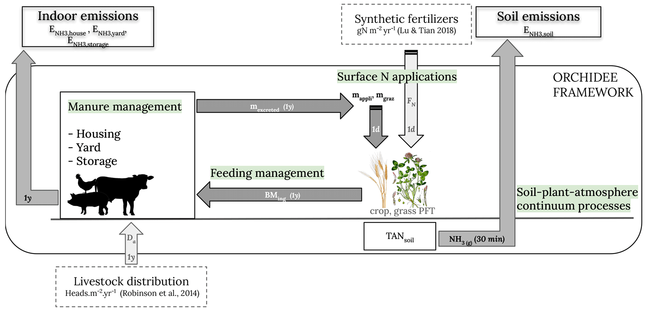
Figure 1Scheme of the agroecosystem representation developed within ORCHIDEE. It is composed of four main components describing feed management, manure management, surface N application, and the soil–plant–atmosphere continuum processes leading to the soil emissions. The livestock distributions and synthetic fertilizers are the main forcing files in the system and are represented in the dashed frames. The time steps (1 year, 1 d, and 30 min) of the processes are indicated using the arrows.
2.1.2 The agricultural N-flow module within ORCHIDEE: CAMEO
Livestock feed management
Both the livestock feeding (BMing, ) and bedding (BMbedding, ) needs are calculated within each grid cell from livestock density distribution maps, for different livestock categories. The livestock types considered in our study are non-dairy cattle, dairy cattle, pigs, small ruminants, and chickens, which are the main contributors to global livestock NH3 emissions. Da, the distribution of each livestock category a, is taken from the Gridded Livestock of the World (GLW 2; Robinson et al., 2014) for the year 2006.
BMing for livestock category a is calculated as follows:
where Wa is the animal weight (kg), and SI is the specific intake (the intake per animal weight unit, ).
A daily dry matter intake equal to 2.5 % of the livestock weight (Paustian et al., 2006) is considered for every livestock category, and a factor of 0.45 is used to convert the dry matter into carbon matter (Paustian et al., 2006), leading to an SI value of 0.01 . Regarding livestock weights, we use regional values adapted from the Supplement of FAO (2018), as listed in Table 1.
Table 1 Regional weights of the animal (kg) used in the intake needs calculation. Data have been adapted from FAO (2018). The regions listed in the table are as follows: NA (North America), RUS (Russian Federation), WE (western Europe), EE (eastern Europe), NENA (Near East and North Africa), ESEA (East and Southeast Asia), OCE (Oceania), SA (South Asia), LAC (Latin America and the Caribbean), and SSA (sub-Saharan Africa).

The livestock feeding and bedding needs are provided by a fraction of the crop and grass NPP which is harvested (called ). In order to quantify the amount of grassland and cropland biomass needed to feed each livestock category (BMing,grass (a) and BMing,crop (a), respectively), we use the fractions of grass and crop that constitute the diet composition of each animal (dgrass (a) and dcrop (a), respectively). The ruminant animals (i.e., cattle and small ruminants) have a diet composed of a portion of grass and crop, whereas the non-ruminant animals (i.e., pigs and chickens) have a crop-only diet. The bedding needs are taken from crop residues only.
The diet composition is calculated from regional feeding information detailed in the Global Livestock Environmental Assessment Model (FAO, 2018) and is described in the Supplement. The bedding is estimated as follows EMEP/EEA (2019):
Here, Strawa corresponds to the amount of straw () used as bedding for each livestock type (Table 2), and the 0.32 factor corresponds to the C content of straw, assuming a C:N ratio of 80 (USDA, 2022) for the straw material and an N content of 4 g N kg−1 (EMEP/EEA, 2019). This value is consistent with recent experimental studies by Su et al. (2020), who found 0.35 kg kg−1 of total carbon in wheat straw.
BMbedding (a) and BMing,crop(a) constitute the total demand for crops. We assume that the demand for crop biomass in each grid cell is satisfied by the amount of crop biomass harvested globally (global market). In contrast, the grass biomass needs are satisfied locally. Indeed, the grass biomass needs define the grassland management intensity through a grazing indicator (GI, unitless) that corresponds to the fraction of grass NPP for the year y that is harvested. Hence, the GI is defined as follows:
where NPPgrass above(y) corresponds to the above NPP of grasslands at the grid cell level (kg C m−2 per grid cell per year) and maxabove, which is a parameter equal to 0.7 and defined as the maximum of the above biomass available for grazing/cutting.
NPPgrass above(y) is a function of the grassland NPP (kg C m−2 per grassland per year) but also of the grassland area defined in each grid cell. Due to an inconsistency between the land use map and livestock density map, the targeted BMing grass value may not be reached by the use of the GI. To ensure that BMing grass demand is always satisfied, we adjust the diet composition of ruminants in some grid cells by increasing dcrop (a) as much as needed (and by reducing dgrass (a) by the same factor). The adjusted value of dgrass (a) is named dgrass, adjusted (a) and is depicted in the Supplement (Fig. S1). The GI is then applied to NPPgrass above(y) on a daily basis in order to obtain the total effective grazed biomass. For each animal, dgrass, adjusted (a) is used to deduce the effective crop biomass from the effective grazed biomass. Finally, each grid cell's effective crop biomass is constrained by the global crop harvested NPP. To do so, we compute the ratio between the global effective crop biomass and the global crop harvested NPP (HI) at a yearly time step. When HI >1, we impose the same constraint locally by dividing the effective crop biomass by HI.
As our methodology is based on an N-flow scheme, the C:N ratio imposed by the model for the crop and grass products is used to convert the carbon into the N biomass ingested (in ). The grassland C:N ratio is unique for each grid cell and varies spatially from 23 to 62, whereas the cropland C:N ratio is fixed for the whole globe and is estimated to be ∼38. BMing tot(y,a) represents the total (including crop and grass products) N biomass ingested, which is used to compute the resulting manure emissions (described in the next section). Concerning the crop used as straw, a fixed C:N ratio of 80 is chosen (EMEP/EEA, 2019).
Indoor N flows and ammonia emissions
We adapt the scheme developed by Dämmgen and Hutchings (2008) which defines indoor ammonia emissions for each animal category. These pathways have also been used in the Tier 2 methodology of the manure management part of the EMEP/EEA Air Pollutant Emission Inventory Guidebook EMEP/EEA (2019). It is based on an N-flow model with mass transfers and emissions proportional to the TAN.
The main output of this module is the N emissions that occur during housing, yarding, and storage of animals, along with the resulting manure produced. The seasonal variability in indoor N emissions is neglected, and the emissions and the manure flow are calculated yearly.
Firstly, we compute the N biomass excreted by each animal category (mexcreted) based on the excretion rates estimated by Paustian et al. (2006) for the Intergovernmental Panel on Climate Change (IPCC) Tier 2 recommendations (see Table 2).
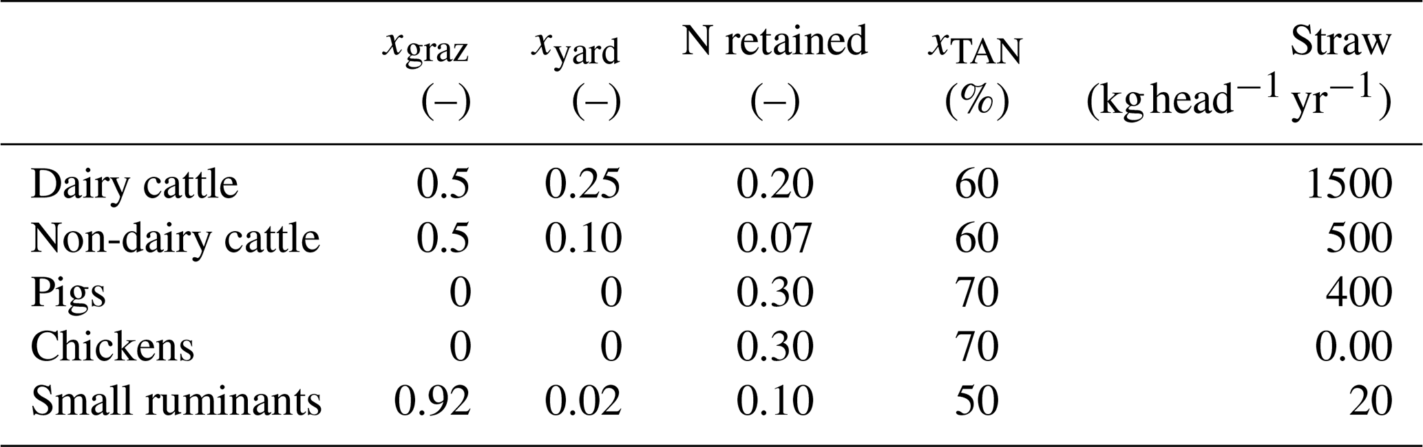
Secondly, we compute the manure excreted during the different livestock activities as a proportion of the year spent in housing, in the yard, and grazing, based on EMEP/EEA (2019). The fraction of time spent in the yard (xyard, Table 2) is prescribed. The remaining time fraction is split into grazing (xgraz, Table 2) and housing periods.
Default values of the TAN fraction contained in the excretal N (xTAN,a) from the manure management part of the EMEP/EEA Air Pollutant Emission Inventory Guidebook 2019 (EMEP/EEA, 2019) (see Table 2) are used to calculate the amount of TAN produced during each activity, i (housing, yarding, and grazing):
Table 2 Default values for the fractions of the year spent grazing and in the yard, the proportion of TAN in the N mass retained, and the straw used as bedding. The information has been taken and adapted from EMEP/EEA (2019). The straw used as bedding for pigs is the average between different livestock types. The N retained is taken from Paustian et al. (2006).
mTAN (graz,a) and mN (graz,a) are used in Sect. 2.1.5 for N application on cultivated areas.
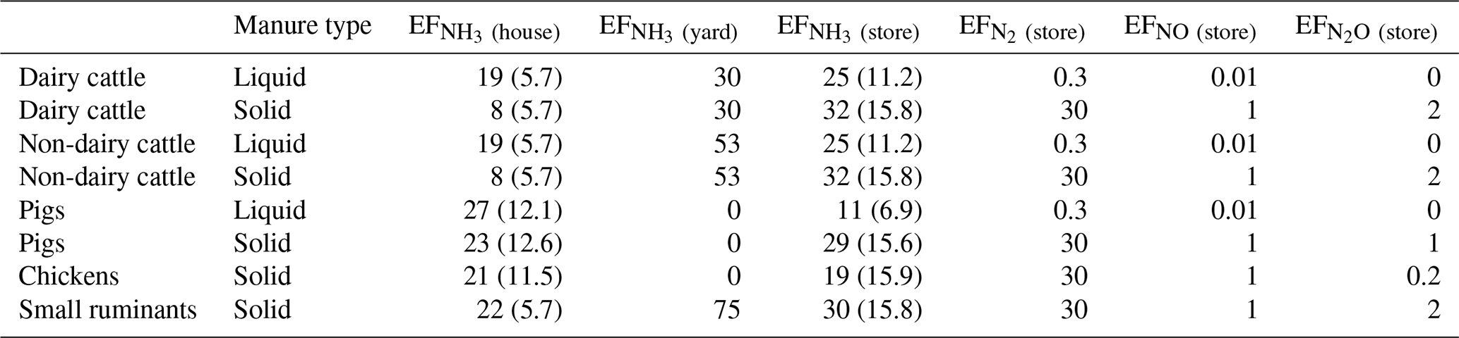
The ammonia emissions from housing (in ) combine the volatilization from liquid and solid TAN masses, with specific emission factors: (kilograms of NH3-N per kilogram of TAN) and (kilograms of NH3-N per kilogram of TAN). and values are taken from Sommer et al. (2019) for each animal a except for the small ruminants category, which is assigned a value from EMEP/EEA (2019) (see Table 3). is written as follows:
where xliq,a (unitless) is the proportion of manure handled as liquid for livestock type a, adapted from the Global Livestock Environmental Assessment Model (FAO, 2018) (see Supplement).
Emissions from yarding () are calculated from the mass excreted in the yard, and there is no distinction between liquid and solid handling.
Table 3 Emission factors (EFs) given as a percentage of the TAN content in the manure. EFs for the yard and the other N species come from EMEP/EEA (2019). The other EFs are taken from Sommer et al. (2019). There is no distinction between liquid and solid manure for yard EFs. Numbers in parentheses are the standard deviations given in Sommer et al. (2019) and used for the sensitivity analysis.
We compute the amounts of N and TAN that are stored as liquid and solid before application ( and for type=liq,sol, respectively; ; Eq. 10). For storage, we assume that all of the manure from housing and yarding is stored, except the N lost by ammonia emissions in the house and yard ( and , respectively). Manure from yarding is considered liquid and goes in the liquid manure storage. Concerning the liquid storage (i.e., slurries), a fraction fmin of the organic N (N-TAN) is converted into TAN through mineralization. A value of 0.1 is used for fmin (Dämmgen and Hutchings, 2008; EMEP/EEA, 2019). For solid storage, we account for an additional N source from bedding (). Incorporation of bedding in the manure storage induces an immobilization of TAN in the organic matter when manure is handled as straw-based solid manure, at a rate fimm proportional to . An fimm value of 0.0067 kg kg−1 is used (Kirchmann and Witter, 1989; Webb and Misselbrook, 2004; EMEP/EEA, 2019). This immobilization greatly reduces the resulting NH3 emissions.
Here, mbed,N is the N mass of bedding (), and mbed is the dry matter mass of bedding.
Manure from storage is supposed to be entirely used as fertilizer. The quantities mTAN (applic) and mN (applic) are the respective TAN and N manures that will be applied to the surface, as described in Sect. 2.1.5. They are obtained by removing the total N emissions from the stored manure (Eq. 11).
In addition to emissions of NH3, other N species (N2O, NO, and N2) emissions can occur from storage and, thus, are required to calculate the final manure mass from storage. These emissions are obtained using the EFs listed in Table 3 as follows:
The remaining manure after storage m(applic,a) and the manure produced during grazing m(graz,a) are the main output of this specific module. Both quantities are the input for the surface application component of the model (described in the next section).
Robinson et al. (2014)FAOSTAT (2020)FAO (2018)FAO (2018)EMEP/EEA (2019)Paustian et al. (2006)EMEP/EEA (2019)EMEP/EEA (2019)FAO (2018)EMEP/EEA (2019)Sommer et al. (2019)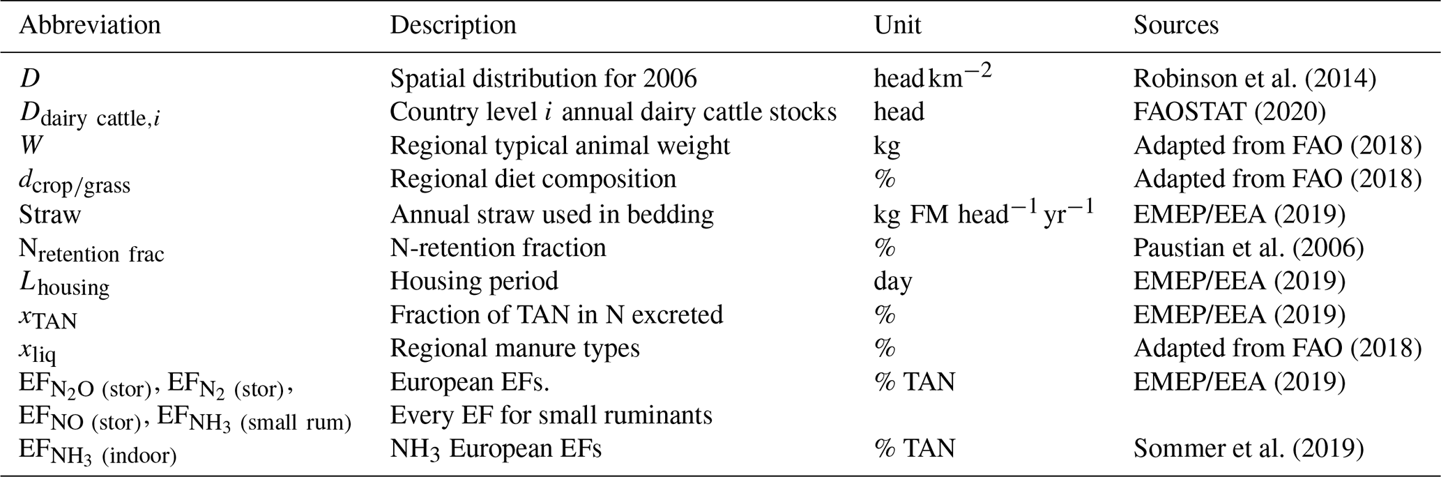
Organic application onto land
This section contains the description of the manure application to soil. m(applic,a) and m(graz,a) are the manure remaining after storage and the manure produced during grazing, respectively (a description is given in Sect. 2.1.4). Both are yearly stocks applied daily at a constant rate and during a specific period, driven mainly by environmental conditions, as described below. This assumption may neglect the actual seasonal patterns of N application usually defined by local governance in some regions. For instance, as discussed in Van Damme et al. (2022), the time of the year when fertilizers can be applied in Europe is strongly dependent on local regulations. Synthetic fertilizers are also considered in our representation and follow the same temporal distribution as the manure from storage. Note that ORCHIDEE does not differentiate between natural and managed grassland. Only grid cells with either the presence of livestock or fertilizer application are considered for the emission calculation, so we can assume that the pixel is managed.
As previously stated, the following two types of manure are considered:
-
Manure from storage and applied to soil as fertilizer. The manure from storage is applied daily at a constant rate for 6 months from the beginning of vegetation growth, corresponding to the first leaf development depending on the PFT. The intermediate period of application (Lapplication=6 months) has been chosen in order to account for the heterogeneity in the agricultural practices, as the model only represents C3 and C4 crop types within the grid cell. Moreover, there is a lack of information in the literature about N application onto grassland at the global scale. We assume that cropland and grassland PFTs receive stored manure with a 2 times higher preference for cropland fractions.
-
Manure deposited during grazing activity by the ruminants. The manure from grazing activity m(graz,a) is calculated in Eq. (7) and is assumed to be only deposited on grassland PFTs by ruminants. The first day of manure deposition for grazing also corresponds to the beginning of vegetation growth. The amount and period of manure deposited during grazing are animal-specific and are determined by the fraction of time passed grazing (xgraz,a).
The soil–plant–atmosphere processes leading to soil emissions
In this section, we describe the physical processes in the soil that influence ammonia emissions. A single soil TAN pool (TAN(soil), g N m−2) is considered. The soil TAN pool is dynamically updated depending on the processes implemented in the model. These processes are described in Zaehle and Friend (2010). The processes corresponding to the creation of are related to mineralization, N application, and NHx deposition, whereas the losses include nitrification, leaching, and volatilization.
TAN(soil,aq) corresponds to the ammonium pool TAN(soil), which is assumed to be diluted in the soil water at a different heights in the soil according to the zactivity parameter.
The zactivity parameter is regulated by all TAN sources, called “input” (“min” – mineralization, “dep” – deposition, BNF, “fert” – mineral fertilizer, and “manure” – applied manure and manure from grazing), in soil as follows:
where inputtot denotes the total TAN sources in soil. We assume that the fertilization and the application of manure are surface N additions to soil, whereas the other sources of TAN (mineralization, deposition, and BNF) are deeply added into soil (pzact_deep=1.0 m). It is worth noting that inputfert is given as the ammonium content of the total N mineral fertilizer applied (the parameter is the fraction of the ammonium content of the N fertilizer used to make the conversion, and this parameter is tested in the sensitivity analysis).
pzact_surf is obtained as described in Riddick et al. (2016):
Here, SWC is the soil water content computed by ORCHIDEE, sW(m) is the specific water volume of manure ( m3 of water per gram of nitrogen; Sommer and Hutchings, 2001; Riddick et al., 2016), and sW(f) is the specific water volume of synthetic fertilizers. sW(f) depends on the soil temperature Tg and is given by United Nations Industrial Development Organization (UNIDO) (1988):
The emissions of NH3 (, ) are obtained following the resistive scheme used in the FAN model (Riddick et al., 2016; Vira et al., 2020):
where NH3(g) is the NH3 concentration at the surface (g N m−3), χa is the free-atmosphere concentration (g N m−3), Ra(z) is the aerodynamical resistance (s m−1), and Rb is the quasi-boundary-layer resistance (s m−1).
χa is prescribed as a monthly field averaged over 11 years from a run of the global LMDZ-INCA (Laboratoire de Météorologie Dynamique–INteraction with Chemistry and Aerosols) model at a resolution (39 vertical levels) over the 2005–2015 period (Hauglustaine et al., 2014). The spatial distribution of χa is presented in Fig. S4 (Supplement) for both May and December (2005–2015 climatology).
Ra(z) is computed interactively by the biophysics module of the ORCHIDEE model. Rb has been implemented according to Xu et al. (2019) as follows:
where is the molecular diffusivity of NH3 in air (m2 s−1; Massman, 1998), c is an empirical constant equal to 3, l is the leaf width (0.02 m; Massad et al., 2010), v is the kinematic viscosity of air (1.56×10⁻⁵ m2 s−1 at 25 ∘C), T is the air temperature (in K), and LAI is the leaf area index (m2 m−2), which is computed by the ORCHIDEE model. The resulting annual mean Rb ranges between 0 and 1.14 s m−1 over the globe. is a function of temperature and is written as follows:
Henry's law coefficient (KH) and the dissociation constant of in water () (Sutton et al., 1994) are used for the speciation between the different TAN species ().
By combining Eqs. (19) and (20), we can compute the gaseous phase of ammonia NH3(g), which is the fraction that will be volatilized. TAN(soil,aq) corresponds to the aqueous phase of TAN in the soil, which is modulated by the height of the soil through the zactivity parameter.
where θ is the volumetric soil water content (in cubic meters of water per cubic meter of soil), and ϵ is the fraction of the air-filled soil volume computed by the ORCHIDEE model.
Kfact is calculated as
and KH, Henry's law constant for NH(3), depends on the surface temperature Tg as follows:
where Tref is the reference temperature (298.15 K), and H is a conversion factor equal to 4.905. We use the value of 0.59 described in Sander (2015) by which the perfect gas constant has been multiplied in order to get a unitless constant. is the dissociation equilibrium and also depends on the surface temperature Tg as follows:
The hydrogen ion concentration [H+] is assumed to be constant and equal to 10−7, which approximately corresponds to the pH given in Massad et al. (2010) for cattle manure, diammonium phosphate fertilizers in acidic soils, and ammonium nitrate fertilizers. A pH of 7 is also adopted in Riddick et al. (2016). In our simulations, the pH does not impact the surrounding soil pH in the model, in contrast to Vira et al. (2020), where the pH varies according to different TAN age classes.
2.2 Modeling setup
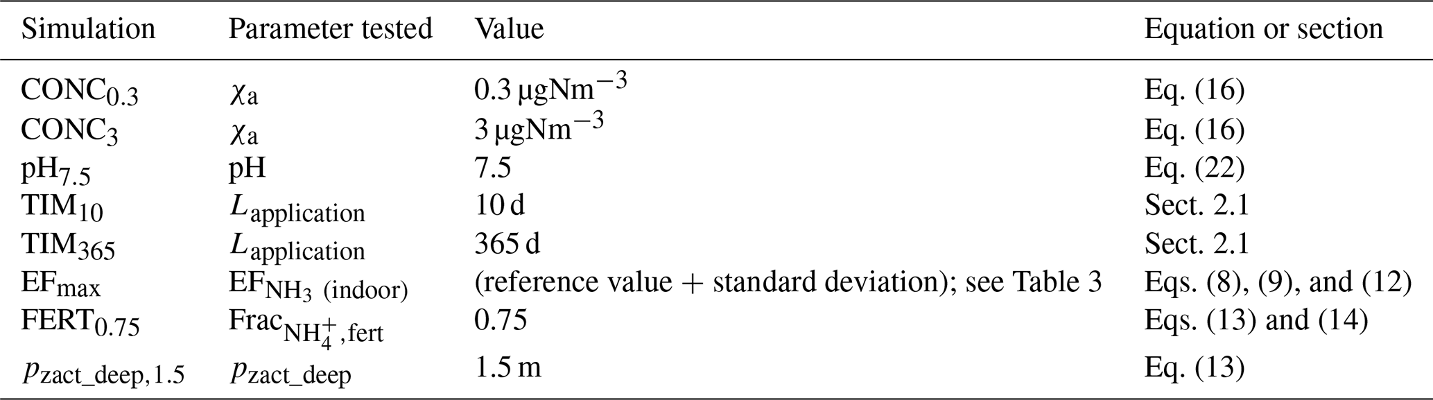
The ORCHIDEE model, including all of the developments described in Sect. 2, was run at a spatial resolution of 2∘ (180×90). This spatial resolution is relatively low but enables one to perform an ensemble of sensitivity tests at a reasonable computing cost. We also performed a reference simulation at a 0.5∘ resolution to ensure that the model resolution does not affect the results. We performed a 10-year reference simulation over the 2005–2015 period. This simulation starts in January 2005 from a simulation done with an ORCHIDEE version similar to the one presented in this paper but without the developments presented in Sect. 2.1.2. In the reference simulation, all annual forcing data are updated every year except those related to BNF and the livestock density, which are constant over time. A set of nine sensitivity test simulations characterized by specific changes in the parametrization were conducted to evaluate the impact of parameter uncertainty on agricultural ammonia emissions. The parameters that have been tested are the atmospheric ammonia concentration (χa), the pH of the manure (pH, default value of 7), the timing period of N application (Lapplication, default value of 183 d), the emission factor for housing and storage activities (), the fraction of ammonium in fertilizer (, default value of 0.6), and the N deep processes regulation parameter (pzact_deep, default value of 1 m). Table 5 summarizes the set of simulations and the key parameters tested.
In Riddick et al. (2016), the value of χa was set to 0.3 µg N m−3, as it is representative of the concentration over low-activity agricultural sites (Zbieranowski and Aherne, 2012). Little sensitivity of the emissions to this parameter was found because χa is much smaller than NH3(g). However, this parameter has been tested in our implementation through a sensitivity analysis.
Table 5 Summary of the simulations performed and the parameters tested. The parameter is described in Sect. 2.1.4 for housing and storage emissions. The equations and sections related to the individual parameters are also indicated.
The ORCHIDEE model requires the following set of forcing data:
-
meteorological data, including the near-surface air temperature and specific humidity, wind speed, pressure, short- and long-wave incoming radiation, rainfall, and snowfall, from the Climatic Research Unit (CRU) and Japanese reanalysis (JRA) dataset (CRU-JRA V2.1) (Harris et al., 2014) (preprocessed and adapted by Vladislav Bastrikov, LSCE, July 2020), provided at 6 h time steps;
-
the global average annual atmospheric CO2 concentration, which is provided by TRENDY (Le Quéré et al., 2018);
-
the global annual land cover distribution, based on combined information from the Land-Use Harmonization 2 (LUH2v2) dataset at a 0.25∘ resolution (Hurtt et al., 2020) and the ESA (2022) CCI Land Cover (see Lurton et al., 2020, for more details);
-
atmospheric N deposition fluxes (NHx and NOy) from the IGAC/SPARC Chemistry-Climate Model Initiative (CCMI; Eyring et al., 2013), which have been used in the N2O Model Intercomparison Project (NMIP) project (Tian et al., 2018), corresponding to information at a 0.5∘ spatial resolution and a monthly temporal resolution;
-
the annual mineral fertilizer rates over croplands and grasslands from an annual dataset developed by Lu and Tian (2017), which corresponds to a reconstruction from 1960 to 2014 for the global cropland matched with the HYDE 3.2 cropland distribution;
-
the biological nitrogen fixation rate, which is provided as climatological data as a function of the evapotranspiration flux (see Vuichard et al., 2019, for more details);
-
the distribution of each livestock category, which is taken from the Gridded Livestock of the World (GLW 2; Robinson et al., 2014) and represents the gridded animal densities (Da) for the year 2006 at a 1 km resolution. Small-ruminant densities correspond to the sum of the sheep and goat densities. The dairy cattle distribution has been retrieved from the total cattle distribution combined with national dairy cattle densities given by FAOSTAT (2020). The calculation adopted is described in the Supplement.
2.3 Model evaluation dataset
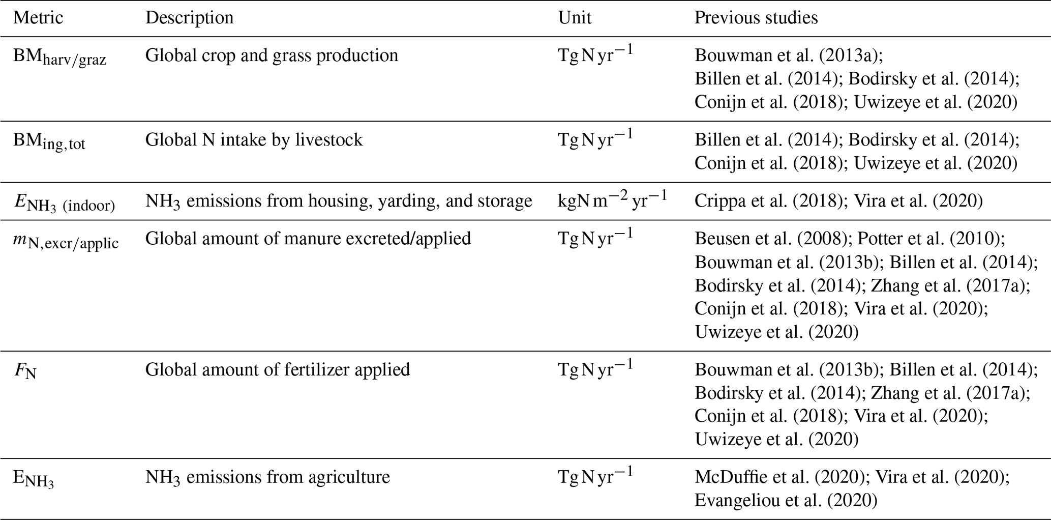
Our integrated approach allows the computation of different variable levels before the final emission results, such as biomass productivity, animal excretion rate, and manure production. This set of variables offers the advantage of evaluating our emissions at different stages of the N flow against the previous works listed in Table 6.
Bouwman et al. (2013a)Billen et al. (2014); Bodirsky et al. (2014)Conijn et al. (2018); Uwizeye et al. (2020)Billen et al. (2014); Bodirsky et al. (2014)Conijn et al. (2018); Uwizeye et al. (2020)Crippa et al. (2018); Vira et al. (2020)Beusen et al. (2008); Potter et al. (2010)Bouwman et al. (2013b); Billen et al. (2014)Bodirsky et al. (2014); Zhang et al. (2017a)Conijn et al. (2018); Vira et al. (2020)Uwizeye et al. (2020)Bouwman et al. (2013b); Billen et al. (2014)Bodirsky et al. (2014); Zhang et al. (2017a)Conijn et al. (2018); Vira et al. (2020)Uwizeye et al. (2020)McDuffie et al. (2020); Vira et al. (2020)Evangeliou et al. (2020)Table 6 Summary of the different simulated variables evaluated in this work by comparison with previous studies.
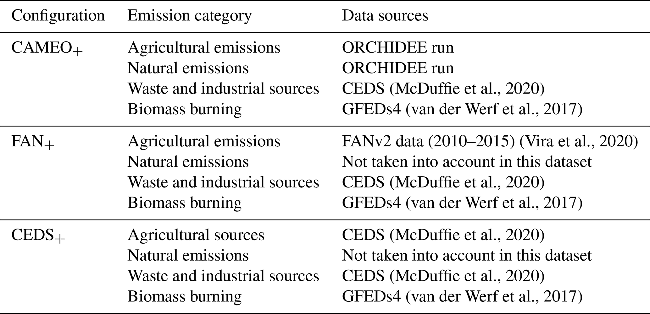
The decadal mean (2005–2015) values of global and regional calculated agricultural emissions, including indoor and soil emissions, are compared to the CEDS inventory (McDuffie et al., 2020) and the emissions simulated by FANv2 (Vira et al., 2020). From the LMDZ–ORCHIDEE–INCA coupling development perspective, it is interesting to compare our approach with CEDS (McDuffie et al., 2020), as it is a reference dataset offering a long period of data (1750–2019). FANv2 has been chosen for our evaluation because our work is based on a similar approach. The regional budget accounts for Africa; tropical southern Asia; Europe; China, Korea, and Japan (abbreviated as China–K–J in the figures); Oceania; India; the USA and Canada; and Latin America. The seasonal variations in ammonia emissions are also evaluated against satellite-derived emissions (Evangeliou et al., 2020). For that purpose, atmospheric NH3 columns observed by the Infrared Atmospheric Sounding Interferometer (IASI) satellite have been combined with the NH3 lifetime calculated by LMDZ-INCA in order to retrieve emissions. The NH3 retrieval product used to derive emissions in our study comprises the 2011–2015 morning observations (Metop-A and -B) and follows a neural network retrieval approach (ANNI-NH3-v3R), as referred to in Van Damme et al. (2017, 2021). Both the lifetime and atmospheric columns are monthly products and share the exact same grid resolution (LMDZ-INCA grid resolution at ). All three CAMEO, CEDS, and FANv2 seasonal variations are evaluated against IASI-derived emissions (defined as IASIinv). In order to be consistent with IASI observations (where no source distinction is possible), the CAMEO, CEDS, and FANv2 agricultural emissions need to be complemented by fire emission data taken from van der Werf et al. (2017) (Global Fire Emissions Database, GFED s4) as well as by industrial and waste sources (McDuffie et al., 2020). The extended emissions are referred to as CAMEO+, FAN+, and CEDS+, respectively, as described in Table 7. It is important to note that only the ORCHIDEE model can provide natural emissions; this source is not considered in the FAN+ nor the CEDS+ datasets.
(McDuffie et al., 2020)(van der Werf et al., 2017)(Vira et al., 2020)(McDuffie et al., 2020)(van der Werf et al., 2017)(McDuffie et al., 2020)(McDuffie et al., 2020)(van der Werf et al., 2017)Table 7 Summary of the different datasets used in the comparison with the IASI-derived emissions. All of the emission sets (except FANv2 data, which are a 2010–2015 climatology) are taken from the 2011–2015 period and have been gridded onto the LMDZ-INCA default resolution of 144×142 pixels.
3.1 Evaluation of intermediate variables
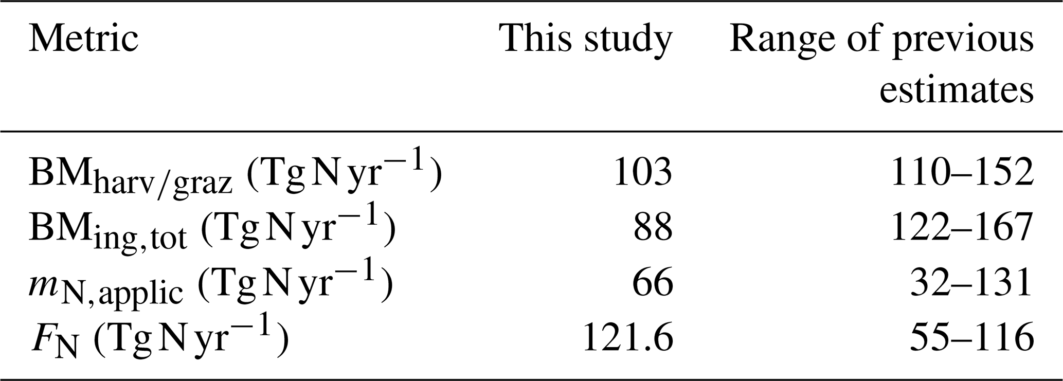
Using the ORCHIDEE model, we estimate the total biomass produced, including grass and crop, to be about 103 Tg N yr−1, which is slightly lower than previous estimates (110–152 Tg N yr−1 estimated by Bouwman et al., 2013a; Billen et al., 2014; Bodirsky et al., 2014; Conijn et al., 2018; Uwizeye et al., 2020). The calculated global annual crop production (expressed in N) is about 74 Tg N yr−1 and compares well with the 72 and 74 Tg N yr−1 estimated by Billen et al. (2014) and Zhang et al. (2021), respectively. The calculated annual grass production (28.8 Tg N yr−1) is more than 3 times lower than the 80.3 Tg N yr−1 reported by Billen et al. (2014) and estimated from the difference between livestock ingestion and available feed resources. By doing so, uncertainties from several components (crop production, net import of vegetal proteins, and human consumption of vegetal proteins) are accumulated. Our resulting total biomass ingested by the livestock (88 Tg N yr−1) is lower than the range found in the literature (122–167 Tg N yr−1; Billen et al., 2014; Bodirsky et al., 2014; Conijn et al., 2018; Uwizeye et al., 2020) which can be attributed to the low grassland production calculated in our model.
However, if the grass N production is largely underestimated by ORCHIDEE, our grass C production estimate of 1.2 Pg C yr−1 is close to the value of 1.95 Pg C yr−1 reported in the Fifth Assessment Report (AR5) of the IPCC (Smith et al., 2014). In this respect, an overestimation of the C:N ratio may also explain part of the grass N production underestimation. It can be explained using a unique grass C:N ratio per pixel and a global C:N ratio for crop in the model. Because we assume that all of the manure stored is then applied to soil, for the evaluation phase, we only consider data from the literature that estimate the application rate of manure to soil. The global annual amount of manure application (66 Tg N yr−1) is lower than the range of 99–129 Tg N yr−1 estimated in recent studies (Beusen et al., 2008; Potter et al., 2010; Bouwman et al., 2013b; Billen et al., 2014; Zhang et al., 2017a; Conijn et al., 2018; Vira et al., 2020; Uwizeye et al., 2020).
Figure 2 compares the distribution of the N manure applied with the values retrieved by Zhang et al. (2017a) for the year 2006 in order to be consistent with the reference livestock distribution used in our approach. The spatial distribution of the manure application highlights the main livestock-raising regions, such as China, India, Europe, Latin America, and the USA. It shows good consistency with Zhang et al. (2017a), although it is higher in India, the USA, and Latin America and lower in China and Europe. These differences can be explained by the fact that we use different regional animal weights per livestock category (Table 1), instead of a fixed value as in Zhang et al. (2017a). This induces different N demands for similar livestock and, ultimately, different quantities of applied manure. Indeed, we use recently adapted data for animal weights from FAO (2018), whereas Zhang et al. (2017a) used IPCC guidelines (Tier1 IPCC, 2006; Paustian et al., 2006). For instance, for India, the non-dairy cattle weight is almost 4 times higher, which explains the differences observed in our calculation. Moreover, our study assumes a unique N excretion rate per livestock type and no livestock system distinctions as a simplification.
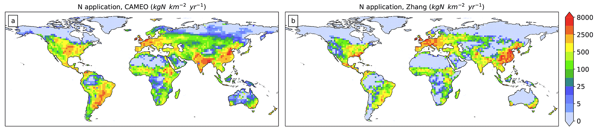
Figure 2The manure application () (a) simulated by CAMEO and averaged over the 2005–2015 period and (b) calculated by Zhang et al. (2017a) for 2006.
Table 8 Global estimates of intermediate variables computed by the model in this study for the 2005–2015 period and the range of previous estimates.
3.2 Agricultural emissions at the global scale
We estimate global NH3 agricultural emissions (averaged over 2005–2015) of about 44 Tg N yr−1: 78 % from soil volatilization (driven by fertilizer and manure application) and the remainder from indoor emissions (from livestock housing, yarding, and storage). These global NH3 emissions are within the range given by McDuffie et al. (2020) and Vira et al. (2020) of 39–47 Tg N yr−1 (Fig. 3a).
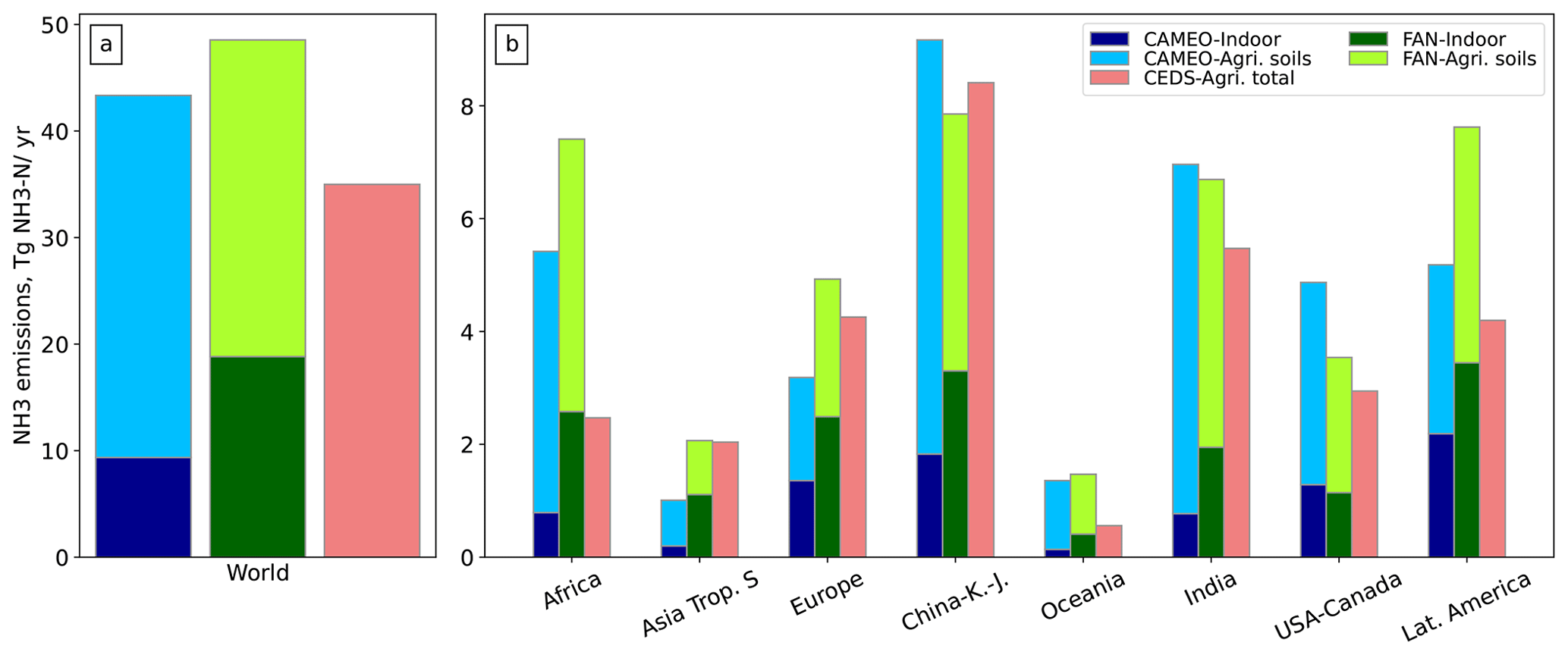
Figure 3Averaged global (a) and regional (b) NH3 emissions (Tg N yr−1) from indoor activities (“Indoor”, darker bars) and agricultural soil (“Agri. soils”, lighter bars) computed by CAMEO over the 2005–2015 period (“CAMEO”, blue bars) and FANv2 (Vira et al., 2020) over the 2010–2015 period (“FAN”, green bars). Total agricultural emissions (accounting for manure management and soil volatilization) estimated in the CEDS inventory (2005–2014 average) (McDuffie et al., 2020) are represented in purple (“CEDS-Agri. total”). China–K–J accounts for China, Korea, and Japan.
China, India, Africa, Latin America, the USA, and Europe appear as the main contributors to global NH3 emissions, accounting for 80 % of the total budget (Fig. 3b). Most of these source areas, which have also been identified as agricultural regions by Van Damme et al. (2018), are regions with intensive crop cultivation (Fig. S2) and important livestock activities, inducing high N application rates (Fig. 2). The spatial distributions of the calculated agricultural NH3 emissions show good agreement with the FANv2 and CEDS results (Fig. 4, b, c). In India and China, our emissions are slightly higher than FANv2 and CEDS estimates. Our values are lower than the FANv2 estimate in Latin America and Africa but high compared with CEDS emissions, which are particularly low in these two regions. In some parts of Africa and Latin America, where the use of synthetic fertilizer is low (never exceeding 2500 ), livestock activity appears to be the main contributor to the emissions.
In intensive agricultural regions, data used for mineral fertilizer application rates can be a source of discrepancy between models. Vira et al. (2020) use the LUH2 dataset (Hurtt et al., 2020), which assumes that only croplands are fertilized. The amounts of fertilizer applied over croplands are comparable globally between Vira et al. (2020) and our study (respective minimum–maximum of 79–87 and 96–101 Tg N yr−1 over 2010–2015) but differ in some regions (see Fig. S2a). In addition, in our study, grasslands are also fertilized with a global amount of 25.7 Tg Nyr−1. This leads to differences in the simulated soil emissions, more specifically in India, the USA, and China, where grasslands are highly fertilized (Fig. S2b) and can be translated into high volatilization rates when compared with FANv2.
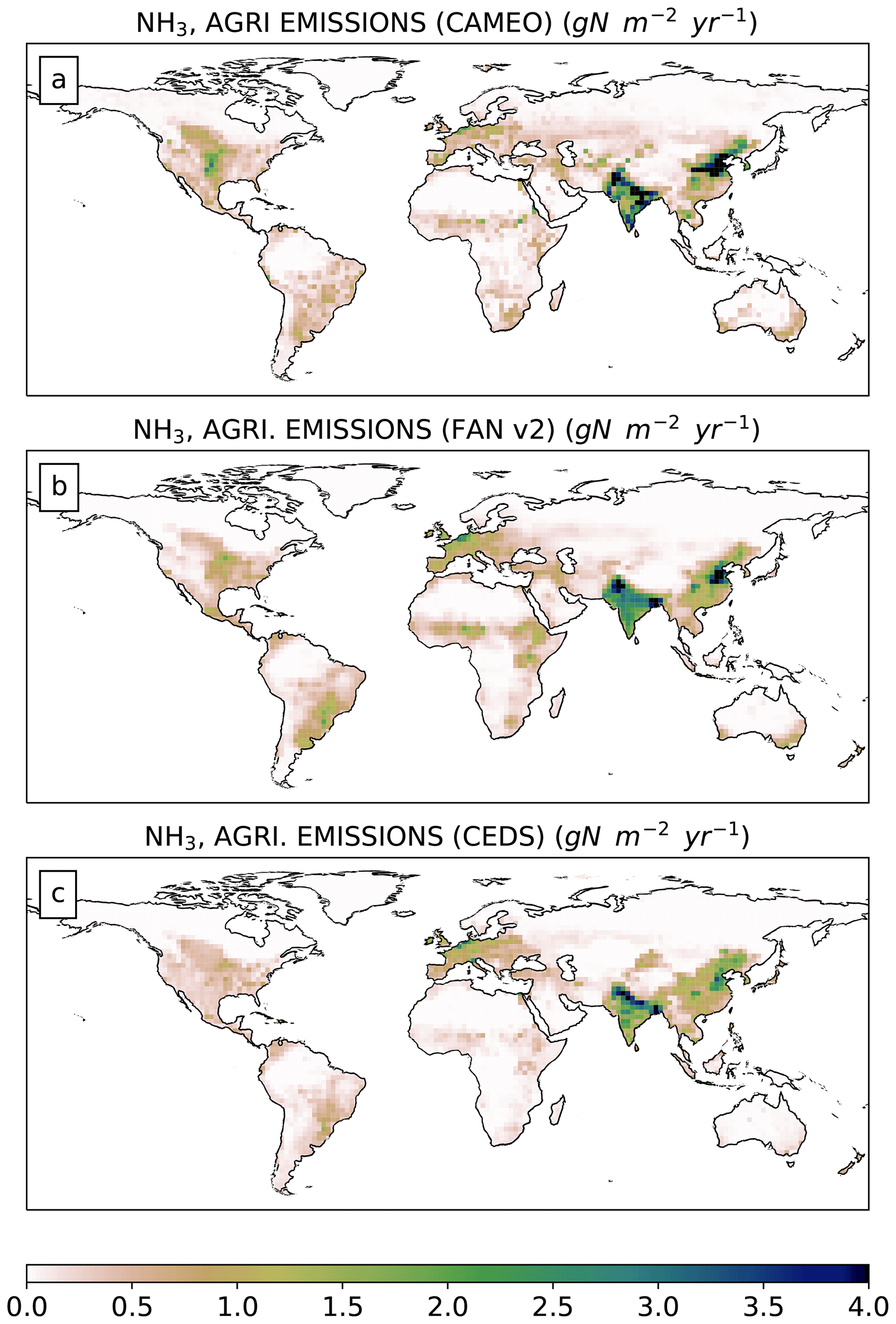
Figure 4Simulated ammonia emissions () from total agricultural sources computed (a) by CAMEO (2005–2015 average), (b) by the FANv2 model (2010–2015 average) (Vira et al., 2020), and (c) from the CEDS inventory (2005–2015 average) (McDuffie et al., 2020).
NH3 emissions peak in June–July–August for most regions (the USA, Europe, China, and Africa; Fig. 5) with maximum values reaching 16.4 in eastern China. The peak in India appears earlier in spring, whereas two peaks occur in Latin America: one during December–January–February and one during September–October–November. Depending on the region, the seasonality of the emissions varies according to different factors, including environmental parameters and agricultural practices. This aspect will be analyzed in more detail in Sect. 3.4 and 3.5.
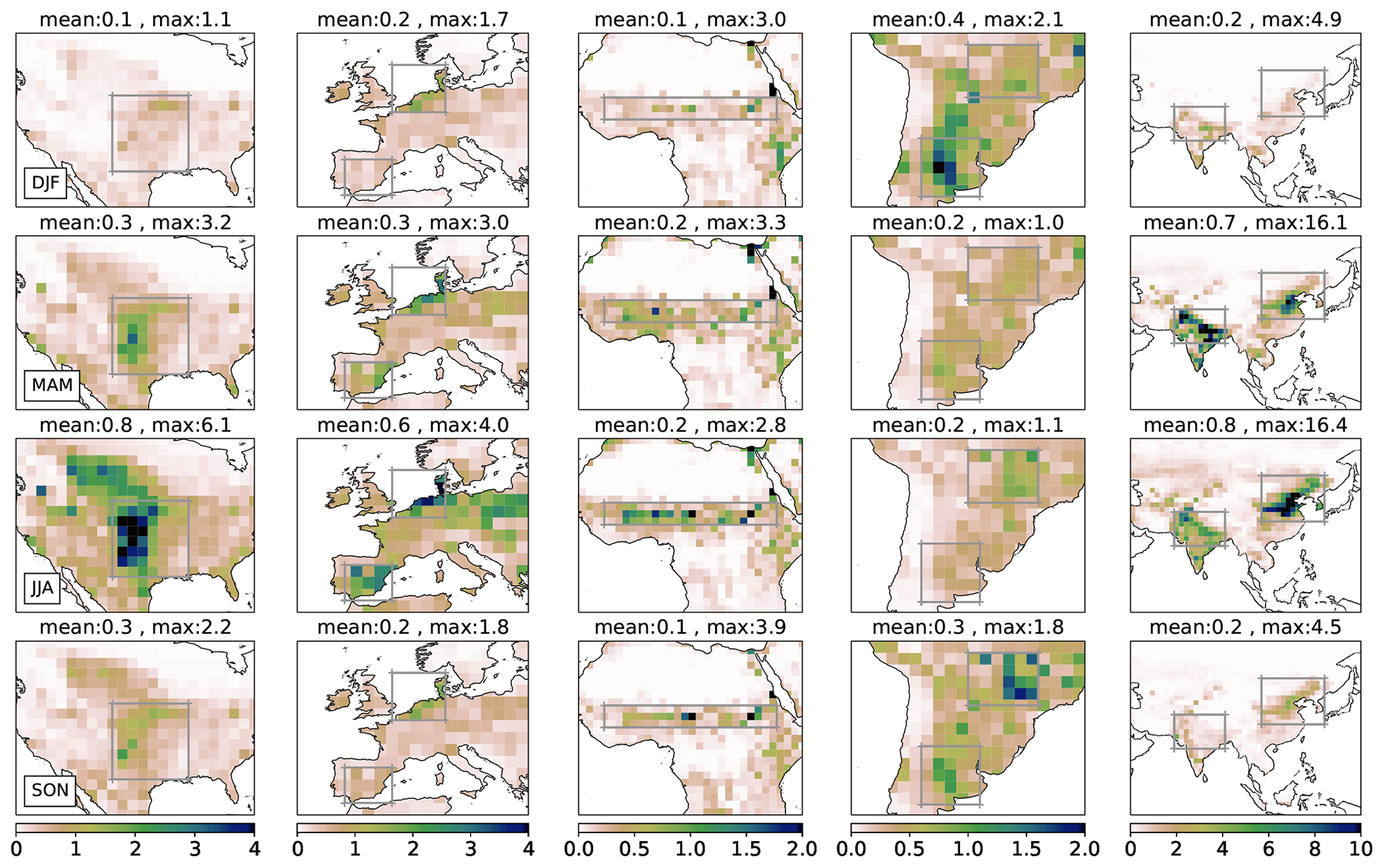
Figure 5Regional seasonal agricultural ammonia emissions averaged over the 2005–2015 period () simulated by CAMEO. Boxes delimit the regions used in the analysis comparing CAMEO emissions with IASIinv (Sect. 3.5). Note that the scales are different for each region.
The spatial pattern of the simulated indoor NH3 emissions (Fig. 6b) is similar to that of manure application rates, with both being driven mainly by livestock density. Hot spot regions of indoor emissions are located in eastern China, eastern India, and northern Europe, with maximum values reaching up to 1.7 . The major sources of volatilization from soils are located in India, eastern China, and the USA, with a maximum value of 12 . The difference in spatial patterns between the two source categories is mainly due to the fact that soil emissions not only depend on livestock distribution (indoor emissions) but also on environmental conditions and mineral fertilizer application rates. The sensitivity of modeled emissions to some of these factors is presented in Sect. 3.4.
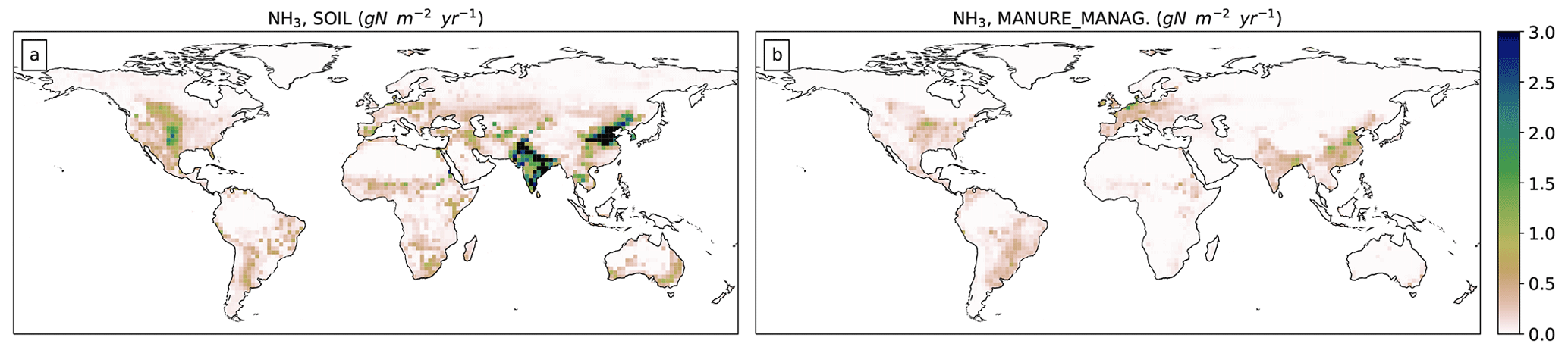
Figure 6Simulated ammonia emissions averaged over the 2005–2015 period () from agricultural soil (fertilizer and manure application) (a) and manure management (b).
The agricultural NH3 emissions from manure management (qualified as “indoor”) are poorly quantified at the global scale. While Vira et al. (2020) reported this emission source to be 18 Tg N yr−1 for 2010, our estimate is half this value (9.6 Tg N yr−1) but is in good agreement with the NH3 emissions reported by Crippa et al. (2018) and Beusen et al. (2008) (9 Tg N yr−1 for the year 2010 and 2000, respectively). Biomass excreted in our model is 40 % lower than what is produced in FANv2, which can partly explain the difference observed in the resulting indoor emissions. In addition, we use EFs from recent studies (Sommer et al., 2019; EMEP/EEA, 2019), whereas a parametrization relying on the temperature and the ventilation rate is used in FANv2 (Vira et al., 2020). However, the parametrization in FANv2 has been adjusted to reproduce default EFs for barns and stores from EMEP/EEA (2016) under European conditions. The use of updated EFs compared with Vira et al. (2020) largely explains the differences between the estimated indoor emission estimates. Moreover, in contrast to FANv2, our manure management module integrates a distinction between solid and liquid manure handling for each livestock type, with very different EF values. As discussed in Groen et al. (2016), Mu et al. (2017), and Uwizeye et al. (2017, 2020), uncertainties associated with EFs are large and can lead to over- or underestimates in indoor emissions and resulting soil emissions. The sensitivity of our calculated total emissions (manure management and soil) to this input parameter will be described in detail in Sect. 3.4, with a change of 14 % at the global scale demonstrating that the parameter has a significant impact on indoor emissions. Furthermore, we consider that each animal category has unique grazing, housing, and yarding periods, whereas Vira et al. (2020) consider regional livestock production systems.
3.3 Emissions at the regional scale
Good agreement is found for the NH3 emissions in China between CAMEO, CEDS, and FAN estimates. In agreement with CEDS, India is the second biggest emitter region (Fig. 3b). However, FANv2 estimates much higher emissions in Africa and Latin America. As mentioned, there are important gaps between estimates given by CEDS and FANv2 for these two regions. In Africa and Latin America, our calculation leads to intermediate results between CEDS and FANv2 estimates.
Our estimates are quite similar to those given by FANv2 and CEDS, especially in Europe, China, and India. However, our indoor emissions are usually lower than what is computed by FANv2, except in the USA, where our emissions are slightly higher. In China, our total agricultural estimate of 9.3 Tg N yr−1 is higher than those from CEDS and FANv2. However, our estimate is lower than those from several studies focusing on Chinese emissions: Kang et al. (2016), Li et al. (2021), Zhang et al. (2018), Crippa et al. (2018), and Zhang et al. (2017b) (9.7, 10.0, 10.3, 11.3, and 12.4 Tg N yr−1, respectively). In India, the emissions that we compute (7.1 Tg N yr−1) are closed to the FANv2 emissions (7.4 Tg N yr−1). Our emissions in North America are 30 % higher than the FANv2 value and the other estimates. As shown in Fig. 6, the southern central part of the USA (mainly Texas) is a hot spot region, where the maximum value can reach 3 . The combination of low soil moisture and a high temperature simulated in this area can explain such high values of volatilization from the soil. In FANv2, emissions do not exceed 1.5 . Unlike the USA, our emissions in Europe are 30 % lower than FANv2 and EDGAR4.3 emissions, whereas they are 15 % lower than EMEP and CEDS emissions.
Unlike in FANv2, where three types of N fertilizers in the form of ammoniacal nitrogen, urea, and nitrates are considered, we assume a constant ammonium fraction of 0.6 in synthetic fertilizers. Even if the yearly fertilizer application is similar to the amount used in FANv2, the ammonium pool in soil from the mineral application can be different. This may imply differences in the emissions, especially in regions where the mineral application is intensive, such as Europe, China, and India (See Fig. S2). Concerning Africa and Latin America, our calculated emissions (∼5.4 Tg N yr−1) are within the range of CEDS and FANv2 values. Africa and Latin America are characterized by specific environmental conditions along with different vegetation types, which may explain the uncertainties present in the estimates. There is also a lack of information regarding agricultural practices and resulting emissions in these regions. In Argentina, Castesana et al. (2018) estimated agricultural emissions of about 0.31 Tg N, whereas our emissions reach 0.91 Tg N and are closer to the estimates of Vira et al. (2020) (1.02 Tg N). The large differences mainly come from fertilizer use, reaching 1400 Gg N in their approach. The fertilizer use from the NMIP project (Tian et al., 2018) (752 Gg N) is in line with the reported values in Castesana et al. (2018) and consistent with the IFASTAT values for 2010–2015 (400–900 Gg N). We can not easily conclude whether the emissions differences come from EFs or manure production estimates. We can only compute a posteriori a single EF for soil emission from our process-based modeling, whereas no manure stock production is given in Castesana et al. (2018).
3.4 Sensitivity to model parameters
Among the parameters tested, the manure pH used in the calculation of the gaseous phase of ammonia is the strongest driver of NH3 emissions (Fig. 7). At the global scale, the pH induces an increase of about 74 % when fixed at 7.5 compared with the reference value fixed at 7.
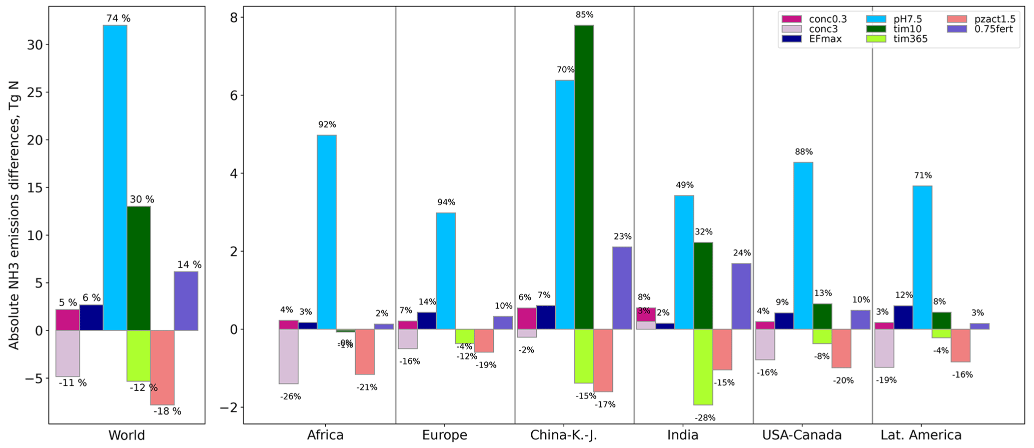
Figure 7Global and regional differences between NH3 emissions from the test simulation (TEST: CONC0.3, CONC3, pH7.5, TIM10, TIM365, EFmax, , and FERT0.75) and the reference simulation (REF) in teragrams of nitrogen (Tg N). Percentages indicate change relative to the REF value: . China–K–J accounts for China, Korea, and Japan.
The impact of the pH is very variable from one region to another: it reaches up to 90 % in some regions such as Africa and the USA, whereas it is the lowest in India (49 %) (Fig. 7). In order to explain these regional differences, we explored the drivers of the spatial distribution of modeled NH3 emission sensitivity to pH. The spatial distributions of the sensitivity of NH3 emissions and the gaseous ammonia pool of the soil to pH are similar (Fig. 8a). In particular, the sensitivity is low in India compared with other regions, like Europe, for both variables. Figure 8b shows the spatial pattern of the dissociation constant of ammonium. The highest values are located in the warmest regions, such as India, where the temperature is one of the main drivers of the dissociation constant. As the dissociation reaction (Eq. 20) is favored in these regions (more NH3 is available), it implies that volatilization is more likely to occur. Along with the high dissociation constant, India is characterized by an important soil concentration (Fig. 8c) due to intensive agricultural input (mineral fertilizer and manure application), leading to a high quantity of TAN being available for emissions. In regions where conditions promote high NH3 volatilization, pH is a weaker driver of emissions. Despite the regional differences in the pH sensitivity, it is an environmental parameter that is an essential driver in the emissions and can be a source of significant uncertainty in our model.
Riddick et al. (2016) also studied the emission sensitivity to pH change. They estimated an increase of 50 % and 70 % in the manure and fertilizer emissions, respectively, when changing the pH from 7 to 8. Even though the sensitivity that we describe seems higher than that in Riddick et al. (2016), no clear conclusion can be reached because we consider a unique pool of TAN. Indeed, we calculate the impact of a change in the total emissions, whereas Riddick et al. (2016) calculated changes in both the manure and fertilizer emissions by changing the pH of the two TAN pools (manure and the fertilizer) separately.
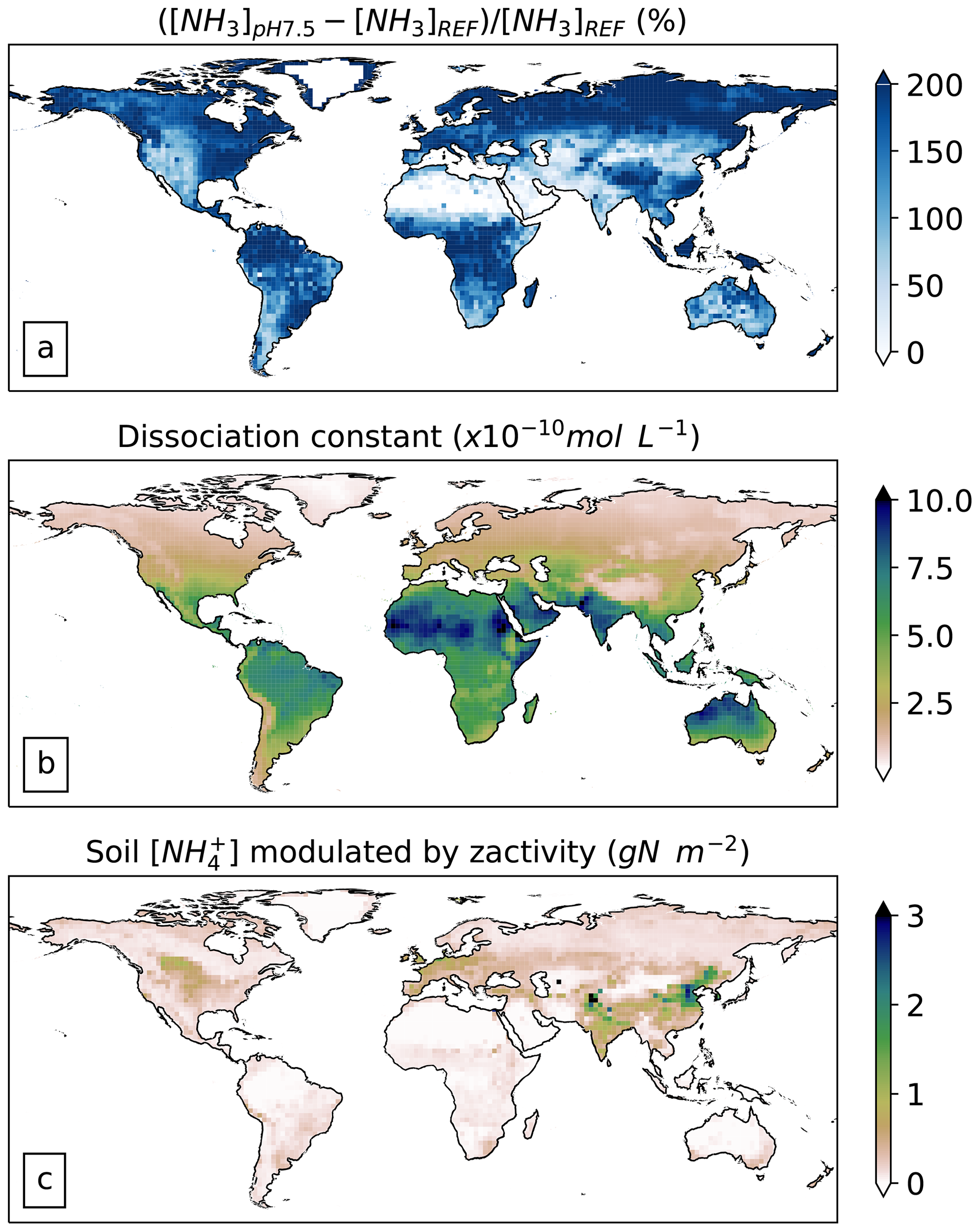
Figure 8(a) The relative anomaly of gaseous ammonia in soil between the pH7.5 simulation and the reference simulation as a percentage (%). (b) The /NH3(aq) dissociation constant from the reference simulation (mol L−1). (c) The soil NH4 concentration modulated by the zactivity parameter (g N m−2).
Changing the duration of the N application (mineral fertilizer and stored manure) from 183 to 10 d induces a 30 % increase in global NH3 emissions. The highest increase is calculated in China (86 %), whereas Europe's impact is slightly negative (−4 %). Reducing the duration of fertilization induces a significant change in the emission dynamic (Fig. 9), with emission peaks occurring right after the start of the vegetation growing season, considered in our model as the first day of the N application period (Fig. 10). However, the emission sensitivity to fertilization duration varies across regions, depending on the environmental conditions after the start of the vegetation growing season. In China, this signal is on average higher in April–May (Fig. 10). It is the period with the lowest soil moisture value and the highest soil temperature, which are conditions that maximize emissions. This could explain the high sensitivity that we observe in this region. On the contrary, in Europe, the growing season signal appears mainly in February and April, when the soil temperature is the lowest and the soil moisture the highest, indicating that these conditions are the least favorable for emissions, resulting in a negative sensitivity.
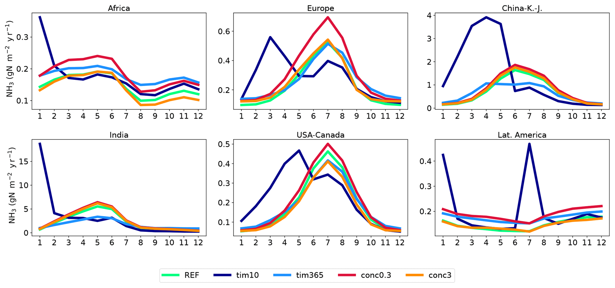
Figure 9Regional NH3 emissions () from different sets of simulations. Green lines are the emissions from the reference CAMEO simulations. Dark and light blue lines are emissions from the respective TIM10 and TIM365 simulations. Dark red and orange lines are emissions from the respective CONC0.3 and CONC3 simulations. China–K–J accounts for China, Korea, and Japan.

Figure 10The regional monthly simulated soil moisture (m3 m−3, in blue) and soil temperature (K, in orange). The regional monthly signal for leaves to start to grow in ORCHIDEE averaged over the different PFTs is drawn using dotted gray lines (this metric is unitless and can be seen as a qualitative signal for the start of the vegetation growing season). Variables are for 2006. China–K–J accounts for China, Korea, and Japan.
When N is constantly applied throughout the year (365 d), the emissions are reduced by about 12 % globally, with India being the region with the strongest reduction (−28 %). The emissions are lower when N is applied throughout the year because it reduces the quantity of N emitted when conditions are the most favorable for volatilization. The variation in pzact_deep from 1 to 1.5 m has a relatively constant impact on NH3 emissions of about −20 % over every region. Increasing pzact_deep increases the dilution of specific ammonium sources (that were assumed to be “deep sources” such as BNF, deposition, and mineralization) in soil, which in turn reduces emissions. Concerning the sensitivity to the content of ammonium in N fertilizers, when is increased by 20 %, emissions increase by about 14 % on average. In China and India, where fertilizer use is the highest, the increase can reach +24 % (see Fig. S5). When fixing the atmospheric concentration at 0.3 and 3 µg N m−3, the global NH3 emissions increase by 5 % and decrease by 11 %, respectively. In Africa, where the impact of using a concentration of 3 µg N m−3 is the highest, emissions are reduced by 26 %, whereas they slightly increase in India (3 %). Indeed, over India, atmospheric NH3 concentrations from LMDZ-INCA are higher than 3 µg N m−3, in particular during May which experiences values up to 7 µg N m−3 (Fig. S4). Counterintuitively, using a fixed atmospheric NH3 concentration (the CONC0.3 and CONC3 simulations) does not induce any important change in the seasonality of emissions (Fig. 9). The sensitivity to this parameter has also been tested in FANv1, and the same range of model response was found (Riddick et al., 2016).
Finally, higher emission factor values imply an increase in total NH3 emissions of about 6 % globally. Although this change is not as significant as other factors, it is worth noting that this impact is only driven by indoor emissions, which account for 22 % of the total emissions globally. In Europe and Latin America, for instance, where the contribution of indoor emissions to the total emissions can reach more than 90 % (Fig. S3), the impact of using higher EFmax values calculated at the scale of these two regions (14 % and 12 %, respectively) is higher than the impact calculated at the global scale.
3.5 Emission seasonality
Seasonality patterns have been first explored by comparing our emissions against the CEDS inventory and the FANv2-simulated emissions. As shown in Fig. 11, we calculate maximum emissions during the spring and summer seasons, whereas the emissions peak almost everywhere only during spring in CEDS and FAN. In the three datasets, the lowest values are calculated during winter, when the meteorological conditions are not favorable for emissions and N application is lowest.
The summer peak observed in our emissions and the spring peak in CEDS and FAN in the USA, more specifically in the central and southern central parts of the USA, are also reported by the Magnitude And Seasonality of Agricultural Emissions (MASAGE) bottom-up inventory from Paulot et al. (2014). In MASAGE, two peaks are highlighted during the year: one in March and the other in June. Goebes et al. (2003) and Pinder et al. (2006) attributed these peaks to the timing of the mineral fertilizer and manure application. This is consistent with our approach, as indoor emissions do not vary over the year and only the N application is time dependent. In Europe, our emissions are higher in summer, whereas Paulot et al. (2014) estimated a clear peak in spring, like in FANv2 and CEDS. In addition, the analysis of Fortems-Cheiney et al. (2020), based on different emission inventories for France, showed the substantial contribution of mineral fertilizer application to emissions, leading to a peak in April. Paulot et al. (2014) demonstrated that April is when emissions reach a maximum over several European agricultural regions, such as Portugal and Spain or Benelux, Germany, and Denmark, due to local regulations preventing farmers from applying manure outside of the growing season. These regions are also characterized by large emissions in July, likely from livestock. This has recently been confirmed by top-down emissions based on Cross-track Infrared Sounder (CrIS) and IASI observation estimates in the UK (Marais et al., 2021). Our approach is constrained by the low level of detail in crop diversity, mainly due to the spatial resolution of the model. Thus, we choose a long enough N application period to catch the crop system diversity. In China, the highest emissions are calculated by our model in summer, which is supported by previous inventories (Streets et al., 2013; Kang et al., 2016; Xu et al., 2018) and satellite observations such as the Tropospheric Emissions Spectrometer (TES) instrument (Shephard et al., 2011) and the Atmospheric Infrared Sounder (AIRS) retrievals (Warner et al., 2017). Our emissions in India peak in spring but remain high during summer. This pattern is also highlighted in the HTAP emissions and IASI satellite data (Janssens-Maenhout et al., 2015; Van Damme et al., 2017), where no strong seasonality is shown over the Indo-Gangetic Plain, but higher emissions are noted from April to September.
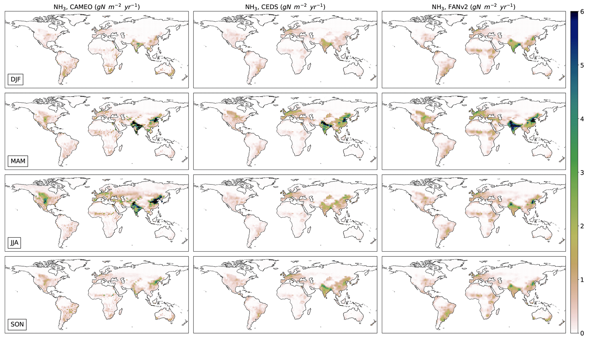
Figure 11Seasonal patterns of ammonia emissions () from total agricultural sources simulated by CAMEO (2005–2015 average, first column), estimated in the CEDS inventory (2005–2015 average, second column), and simulated by the FANv2 model (2010–2015 average, third column).
To complete our analysis, monthly emissions derived from the IASI satellite (IASIinv) averaged over the 2011–2015 period are used as a comparison regarding different hot spot regions defined in Fig. 5. The same operation has been carried out for agricultural emissions from FANv2 and the CEDS inventory, and the details of the CAMEO+, CEDS+, and FAN+ dataset constituents are listed in Table 6. First, it is worth noting that the seasonality of CAMEO+, CEDS+, and FAN+ is primarily due to their respective agricultural emissions; the other sources have no important role in the seasonality. Indeed industrial and waste sources show very low annual standard deviations (in the ranges of 10−7 and 10−8 , respectively) compared with the agricultural emissions estimated by CEDS, FANv2, or CAMEO (0–8 ). Biomass burning emissions have a standard deviation reaching 0.6 in areas characterized by high fire activity, whereas the deviation is intermediate in agricultural regions ( ; Fig. S7). Overall, our emissions seem to be consistent with IASIinv, with the general patterns and the absolute values being similar (Fig. 12), except for the equatorial Africa and central Brazil regions where CAMEO+ largely underestimates IASIinv. Seasonal emission patterns of CEDS+ and FAN+ are quite close to each other but very different from IASIinv. FAN+ and CEDS+ usually depict a sharp peak in spring (1 month in advance in FAN+) as well as another smaller peak only for CEDS+ in September–October. While the seasonality in CEDS+ is artificially retrieved from a specific profile, the temporal variability in FAN+ is driven by the meteorological conditions and the crop types present within the pixel. Even though the representation of crops in version 5.0 of the Community Land Model (CLM5.0) used in FANv2 is more precise than in ORCHIDEE (eight crop types compared with two), we observe that the temporal variability is better represented in our approach when compared to IASIinv. In FANv2, the fertilizer application is triggered 20 d after leaf emergence. This might explain the single sharp peak observed in spring, while the long period (6 months) that we have chosen seems to capture the general pattern of emissions better. More specifically, there is very good agreement between CAMEO+ and IASIinv in the central USA, where emissions peak in summer (>2 ). In Europe, our calculated emissions show a clear and strong peak in July, whereas IASIinv patterns are different. In northern Europe, IASIinv presents two peaks, in March and in August, with very low emissions in winter, whereas emissions remain at around 0.5–0.8 in CEDS+, CAMEO+ and FAN+. These differences might be explained by high uncertainties associated with the IASI instrument during this period. Van Damme et al. (2014) highlighted limitations in the IASI (Metop-A) measurement availability over Europe in winter 2011. The number of cloud-free observations is low, especially in December and January, with only 4 % of the dataset being associated with an error lower than 50 % due to the thermal contrast (defined as the temperature difference between the Earth’s surface and the atmosphere at 1.5 km) and the amount of ammonia present in the atmosphere. In southern Europe (the Spanish region), IASIinv emissions show a weaker seasonal cycle than CAMEO+, peaking in summer. Spain is characterized by a diversity of agricultural production types (e.g., crops, fruits, and olives) which are not differentiated in our model. This highlights a limitation in our approach: the homogeneous representation of agricultural lands causes emissions to have the same seasonal pattern over this region. In the northern part of India, CAMEO+ highlights a peak in May, which is 2 months earlier than the peak in the IASIinv. In agreement with IASIinv results, Tanvir et al. (2019) also depicted a clear peak in the NH3 concentration in July using the TES data for the Indo-Gangetic Plain. It is worth noting that IASI observations in this specific region might be associated with a high level of uncertainties (Marais et al., 2021). Marais et al. (2021) indicated that, in addition to the intense biomass burning season and the relatively low abundance of acidic aerosols in northern India, warm temperatures may increase emissions and suppress the partitioning of NH3 to aerosols, thereby inducing an enhancement in the spectral signal. In the Chinese hot spot, we observe the same peak in summer for both CAMEO+ and IASIinv, even though our maximum value is almost 2 times higher than that of IASIinv (Fig. 12).
In Africa and Latin America, our emissions show a less pronounced variability over the year than IASIinv. Results in Africa show three peaks (February, May, and October) in the IASIinv, whereas our emissions highlight only one peak in June (Fig. 12). Equatorial Africa is a specific region with respect to emission seasonality that has recently been studied in Hickman et al. (2021). The aforementioned work revealed different ecoregion drivers of the atmospheric NH3, explaining the seasonal patterns observed by the IASI satellite. The region chosen in our study is between the two northern ecoregions, wet and dry savannas, which are characterized by important livestock densities and intense biomass burning activities.
The June peak retrieved in CAMEO+ and IASIinv can be attributed to the seasonal pattern of the dry savanna. This time of the year corresponds to the rainy season in the dry ecoregions, and emissions from soil (from livestock excreta and natural processes) are expected to be stimulated through microbial activity enhanced by precipitation (Hickman et al., 2018). Hickman et al. (2021) demonstrated that precipitation and temperature are the most important predictors to explain the seasonality of the emissions in this region. The two other peaks in the IASIinv during the dry season (February and October) could be a contribution from the wetter region located just below the dry savanna. Hickman et al. (2021) demonstrated that, in addition to the importance of the soil emissions in this region, vegetation fires during this period might explain additional emissions. This result is also supported by the long-term measurements from INDAAF (International Network to study Deposition and Atmospheric composition in Africa), which suggest that the seasonality in the wet savanna is the result of biomass burning, with a high increase in the concentrations during the dry season (Adon et al., 2010). The absence of these two peaks in our estimate can be explained by an underestimation of the biomass burning emissions from the GFEDs4 inventory used to complement our emissions (van der Werf et al., 2017). This inventory is based on MODIS biomass burning area, and recent analysis has suggested that MODIS underestimates fire emissions by a factor of 2–5 due to the non-detection of small fires (Roteta et al., 2019; Hickman et al., 2021; Ramo et al., 2021), mainly from agricultural practices.
The case of Latin America has been much less studied, and we observe strong seasonality in IASIinv. The two regions in Latin America are characterized by croplands, intensive livestock farming, and biomass burning activities. Over central Brazil, IASIinv reveals an important peak in September (>4 ) that is only represented in the CAMEO+ and FAN+ time series by a smooth increase. Andela et al. (2017) has shown a strong positive spatial correlation between burned area and cropland fractions in this ecoregion, probably suggesting significant agricultural waste burning. In addition, Castro Videla et al. (2013) have also shown a maximal biomass burning activity measured by MODIS via the monthly mean number of fires (MODIS fire dataset) in the Brazilian Caatinga shrublands and in the northeastern part of the Cerrado region in September. In the Pampas region, the general seasonality from IASIinv and our emissions describes the highest emissions from September to March and low emissions during the rest of the year. However, our emissions do not highlight the clear peaks in March and September that are shown by IASIinv. The work of Castro Videla et al. (2013) has pointed out sugarcane and soybean expansion in this region as the main drivers of biomass burning. This can lead to the same conclusion as for Africa with respect to the small fires that are often not detected by MODIS and, thus, might be not considered in the GEFDs4 inventory used in our work. It is also worth noting that manure application as a fertilizer is not a common practice in Argentina (Vázquez Amabile et al., 2015). In our approach, all of the manure is applied. This would potentially lead to a distinct seasonal cycle compared with a case in which all of the manure is stored for the whole year.
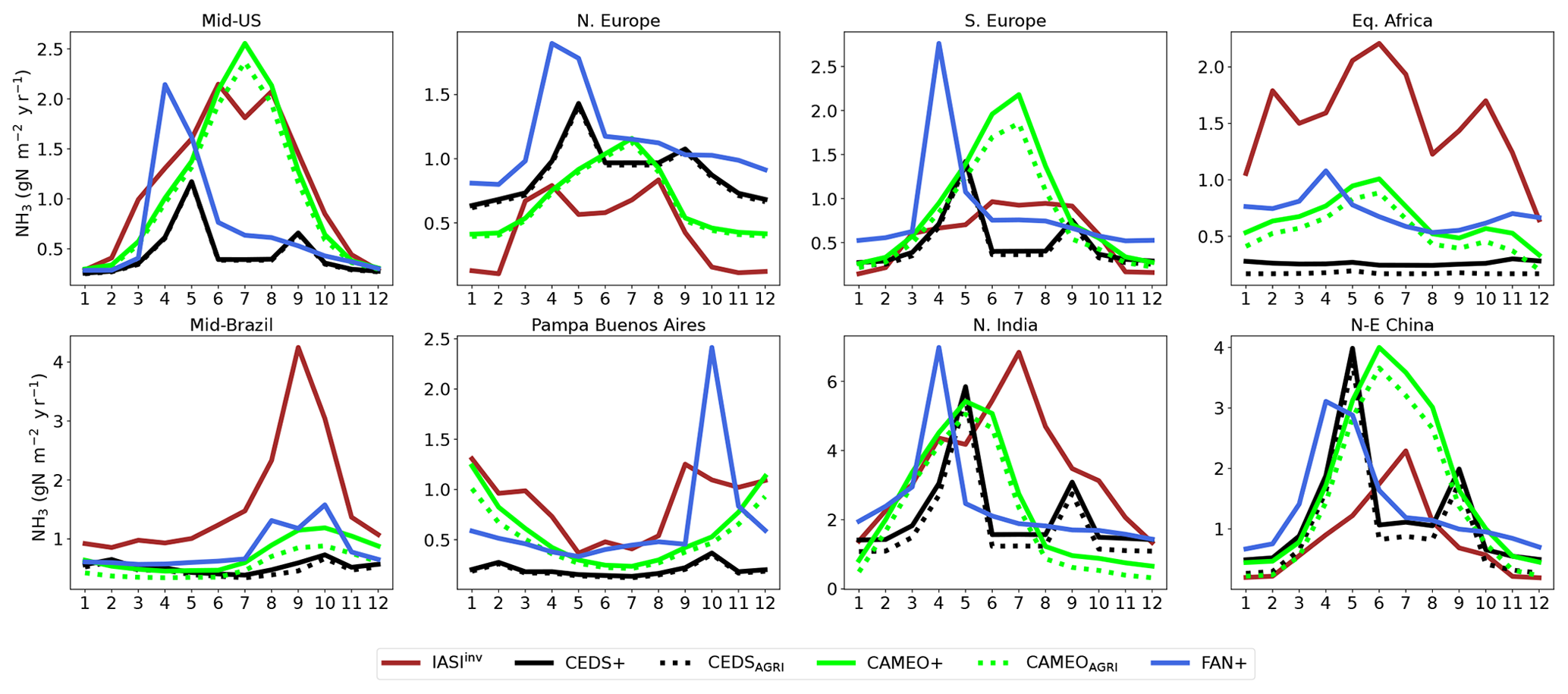
Figure 12Monthly regional NH3 emissions (). The CAMEO emissions accounting for natural and agricultural emissions aggregated with other sources are represented by the solid green line (CAMEO+), and CAMEO emissions accounting for agricultural emissions are shown using the dotted green line (CAMEOagri). The agricultural sector of CEDS alone and CEDS aggregated with other sources are represented by black dotted (CEDSagri) and solid lines (CEDS+), respectively. The IASIinv product is shown in red (IASIinv). The agricultural emissions from FANv2 aggregated with other sources are shown in blue (FAN+). Other sources include biomass burning from van der Werf et al. (2010) and industrial and waste sectors from CEDS. The regions are defined in Fig. 5.
The temporal correlation scores between the reference (here IASIinv) and CAMEO+, CEDS+, and FAN+ calculated over the monthly time series for the 2011–2015 period are plotted in Fig. 13. The results highlight excellent month-to-month agreement with respect to variability between CAMEO+ and IASIinv in most regions of the globe. In the main hot spot regions, such as China, India, Europe, and the USA, correlations are between 0.7 and 0.9, while correlations between IASIinv and CEDS+ and between IASIinv and FAN+ hardly exceed 0.5. This means that our modeling approach enables a satisfying representation of the seasonal cycle in terms of agricultural and natural emissions in comparison with CEDS agricultural emissions, where a forced seasonal profile (two respective high volatilization peaks in May and September) is used, and with the FANv2 model, accounting for a more realistic representation. However, in the southeastern part of the USA and the Chaco region in Latin America, we observe a degradation of the seasonal pattern in our emissions compared with both CEDS+ and FAN+, which show high correlations. The Chaco region is one of the main hot spot in terms of natural soil emissions in our model, as highlighted in Fig. S6. It is characterized by savanna with grasslands, thorn forests, a mosaic of woods with savanna, and shrubs, and coarse grasses predominate (Berry et al., 1995). However, most of the natural emissions computed in ORCHIDEE originate from temperate broad-leaved summer green PFTs. Many studies have demonstrated the importance of the biomass burning events with respect to the emission quantities mainly occurring during the dry season in September–October (Castro Videla et al., 2013; Pereira et al., 2022). IASIinv depicts an important peak in the NH3 emissions (See Fig. S6) during this time of the year which can be attributed to fire events. We observe that natural and agricultural emissions have very similar patterns and are in the same range. However, the fire contribution in the CEDS+ and CAMEO+ datasets appears to be very low, supporting the limitation of using the GFEDs4 inventory in bottom-up NH3 emission estimates for comparison with IASIinv. The degradation of the correlation between IASIinv and CAMEO+ compared with the correlation with CEDS+ in the Chaco region is explained by the fact that there is almost no temporal variability in the CEDS+ at the annual scale.
In India, there is an interesting pattern with a clear longitudinal delimitation – western negative and eastern positive correlations – in CAMEO+ and CEDS+. In the northwestern part of India, CAMEO+ performs better with respect to capturing the IASIinv seasonality than CEDS+ and FAN+.
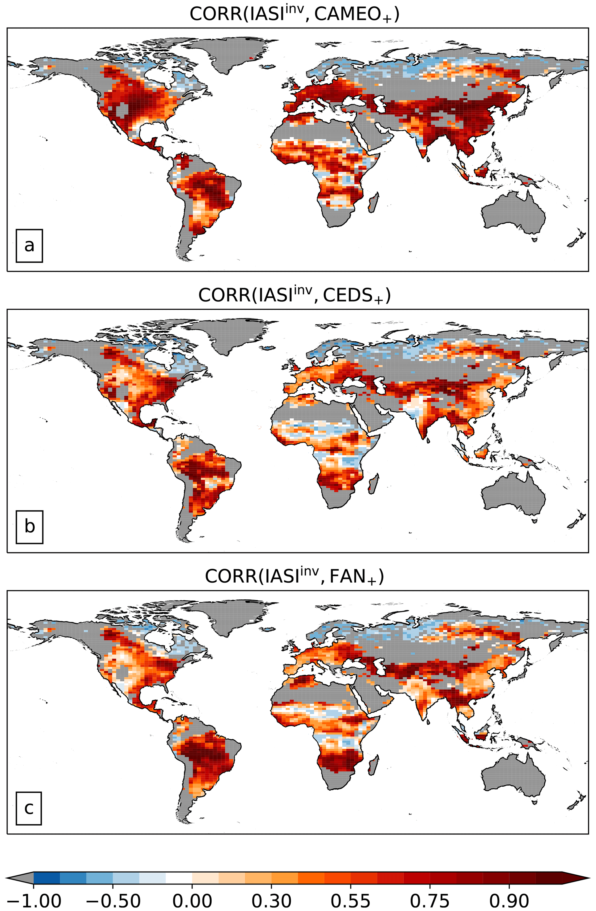
Figure 13Temporal correlation scores between IASIinv and CAMEO emissions aggregated with other sources (a) and between IASIinv and total emissions from CEDS for agricultural, industrial, and waste sources aggregated with biomass burning (b) over the 2011–2015 period. Temporal correlation scores between IASIinv and FANv2 aggregated with other sources are shown in panel (c). Other sources include biomass burning from van der Werf et al. (2010) and industrial and waste sectors from CEDS. Gray grid cells correspond to a standard deviation in the monthly IASIinv time series lower than 0.2 in order to avoid biased correlation scores.
Based on the comparison with the seasonality of IASIinv, there is a strong limitation in using CEDS as NH3 emission information for a CTM in order to study its impact on atmospheric chemistry. More specifically, we demonstrate that using ORCHIDEE land-based emissions has the potential to improve the seasonal signal of the resulting ammonia concentration in the atmosphere.
However, using IASIinv to evaluate our model results also has limitations due to the uncertainties associated with the satellite product and the derivation method. For example, many studies using IASI data do not consider winter observations in the USA nor Europe (Marais et al., 2021) due to a potential degradation of the data because of atmospheric conditions (e.g., cloud cover and low temperatures). The use of the NH3 lifetime simulated by LMDZ-INCA in the inversion method is also associated with uncertainty. Moreover, the interpolation method used to regrid the IASI observations onto the LMDZ-INCA grid can be a source of uncertainties, as demonstrated in Evangeliou et al. (2020).
In this study, we implement a new module dedicated to global NH3 emissions from agricultural practices including livestock waste management and mineral fertilizer application within the ORCHIDEE land surface model. Our development allowed us to consider dynamical variables (such as surface temperature and humidity) through different physical soil processes for the calculation of the NH3 fluxes. This aspect, which is often neglected in bottom-up approaches, is key for a realistic seasonal representation of the emissions. In contrast to other emission models, our module interacts with the ORCHIDEE model for vegetation variables such as the biomass productivity. It allows the calculation of a grazing index, a global indicator of the pressure exerted on the vegetation. We estimate global agricultural emissions of about 44 Tg N yr−1, with soil volatilization from fertilizer and manure application accounting for 78 % of emissions and indoor emissions (from livestock housing, yard and storage) accounting for the remainder. The spatial distribution of the calculated emissions is consistent with previous studies (the CEDS bottom-up inventory from McDuffie et al., 2020, and the process-based model by Vira et al., 2020) highlighting the most important emission regions, such as eastern China, northern India, the USA, and Europe, which are characterized by either a high N application rate or intensive livestock farming.
In order to evaluate the modeled emissions, different sensitivity simulations involving key parameter variations have been performed. The most important parameter driving the emissions is the pH of the N input, which induces an increase of about 74 % for NH3 emissions when shifted from 7 to 7.5. Assuming a constant value for the pH simplifies our approach. Using a soil pH map would imply more complex processes, involving a change in the pH during N application. In addition to the ammonium content, the pH used is rarely available in the literature.
Manure management emissions are also associated with uncertainties due to the use of EFs. Even though EFs are calculated using an extensive definition of livestock and management systems as well as considering variations in climate and management practices, the use of European EFs for the whole globe is an important assumption. However, we demonstrate that the overall emissions are moderately sensitive to the EFs, with a global change of 6 % for emissions when the maximum range given by Sommer et al. (2019) is used. Similarly, regional parameters given by FAO (2018) were simplified to match the representation of the vegetation distribution in ORCHIDEE. Assuming livestock feed is composed of only grass and crop products neglects the use of the agro-industrial by-products, which is standard practice in Europe and the USA. Modeled emissions are also sensitive to the timing of the N application, especially in China, where a shortening of the fertilization period induces very high volatilization rates. Apart from this parameter, none of the other factors tested appear to be important drivers of the emission seasonality. Finally, the seasonality patterns have been further analyzed using satellite-derived emissions. The comparison suggests that ORCHIDEE simulates a very good representation of the seasonality of NH3 emissions, with correlation scores larger than 0.7 in the most important emission regions.
In addition to the gain with respect to realistic seasonality, our approach fills the lack of estimates for emissions from natural soils, which are missing in almost every inventory. This is highly interesting for Africa and Latin America, where these sources are important (Hickman et al., 2018) and not well studied. These encouraging results prove the potential of coupling ORCHIDEE land-based emissions to CTMs, which are currently forced by bottom-up anthropogenic-centered inventories such as CEDS. This framework provides room to improve the representation of the emissions, as atmospheric variables are dynamically simulated by CTMs. For instance, the surface NH3 concentrations used in the final calculation of the emissions could be updated at each time step instead of prescribing an external monthly file for a given climatology. In addition, a tight relationship exists between emission and deposition of NH3, as NH3 is particularly reactive, and deposition of contributes to the reemission of NH3 from natural and managed soils. By coupling emissions with the global LMDZ-INCA CTM through the dynamic calculation of wet and dry deposition, we plan to improve the representation of the emissions as well as the atmospheric concentrations. In addition, a further evaluation will consist of comparisons with atmospheric composition observations.
The ORCHIDEE model is available at https://forge.ipsl.jussieu.fr (last access: 6 February 2023). The modified version of ORCHIDEE including the CAMEO module used in this paper is available at https://doi.org/10.14768/db1cf5ce-6fd2-4b4c-a3d1-598e2283c19d (Beaudor et al., 2022b). The NH3 emissions simulated by CAMEO as well as the manure production data and the soil ammonium concentrations are available at https://doi.org/10.5281/zenodo.6818373 (Beaudor et al., 2022a); other model outputs and the IASI-derived emissions are available upon reasonable request from the authors. The NH3 emission inventories used in this study are available in McDuffie et al. (2020) for the CEDS and at https://doi.org/10.5281/zenodo.3841723 (Vira et al., 2020) for the FANv2 data.
The supplement related to this article is available online at: https://doi.org/10.5194/gmd-16-1053-2023-supplement.
NV, DH, JL, and MB designed the module. NV and MB implemented the module in ORCHIDEE and designed and performed the simulation experiments. MB analyzed the output and prepared the manuscript with contributions from NV, DH, and JL. MVD and LC provided the IASI satellite product and performed the regridding of the data. NE conducted the emission derivation from the IASI product. All of the authors contributed to writing the manuscript.
The contact author has declared that none of the authors has any competing interests.
Publisher’s note: Copernicus Publications remains neutral with regard to jurisdictional claims in published maps and institutional affiliations.
The authors acknowledge support from the ESM2025 project. We also acknowledge support from the GENCI supercomputer system (Joliot-Curie supercomputer). Nikolaos Evangeliou received support from the Research Council of Norway (project ID no. 275407; “COMBAT – Quantification of Global Ammonia Sources constrained by a Bayesian Inversion Technique”). Martin Van Damme was supported by the ARENBERG (“Assessing the Reactive Nitrogen Budget and Emissions at Regional and Global Scales”) FED-tWIN project funded via the Belgian Science Policy Office (BELSPO). Lieven Clarisse is a research associate supported by the Belgian F.R.S.-FNRS.
This research has been supported by the H2020 European Institute of Innovation and Technology (grant no. 101003536).
This paper was edited by Jinkyu Hong and reviewed by two anonymous referees.
Abbatt, J. P. D., Benz, S., Cziczo, D. J., Kanji, Z., Lohmann, U., and Möhler, O.: Solid Ammonium Sulfate Aerosols as Ice Nuclei: A Pathway for Cirrus Cloud Formation, Science, 313, 1770–1773, https://doi.org/10.1126/science.1129726, 2006. a
Adon, M., Galy-Lacaux, C., Yoboué, V., Delon, C., Lacaux, J. P., Castera, P., Gardrat, E., Pienaar, J., Al Ourabi, H., Laouali, D., Diop, B., Sigha-Nkamdjou, L., Akpo, A., Tathy, J. P., Lavenu, F., and Mougin, E.: Long term measurements of sulfur dioxide, nitrogen dioxide, ammonia, nitric acid and ozone in Africa using passive samplers, Atmos. Chem. Phys., 10, 7467–7487, https://doi.org/10.5194/acp-10-7467-2010, 2010. a
Andela, N., Morton, D. C., Giglio, L., Chen, Y., Werf, G. R. v. d., Kasibhatla, P. S., DeFries, R. S., Collatz, G. J., Hantson, S., Kloster, S., Bachelet, D., Forrest, M., Lasslop, G., Li, F., Mangeon, S., Melton, J. R., Yue, C., and Randerson, J. T.: A human-driven decline in global burned area, Science, 356, 1356–1362, https://doi.org/10.1126/science.aal4108, 2017. a
Anderson, N., Strader, R., and Davidson, C.: Airborne reduced nitrogen: ammonia emissions from agriculture and other sources, Environ. Int., 29, 277–286, https://doi.org/10.1016/S0160-4120(02)00186-1, 2003. a, b
Bauer, S. E., Koch, D., Unger, N., Metzger, S. M., Shindell, D. T., and Streets, D. G.: Nitrate aerosols today and in 2030: a global simulation including aerosols and tropospheric ozone, Atmos. Chem. Phys., 7, 5043–5059, https://doi.org/10.5194/acp-7-5043-2007, 2007. a
Beaudor, M., Vuichard, N., Lathière, J., Evangeliou, N., Van Damme, M., Clarisse, L., and Hauglustaine, D.: Global agricultural ammonia emissions simulated with the ORCHIDEE land surface model: Model Ouput Data, Zenodo [data set], https://doi.org/10.5281/zenodo.6818373, 2022a. a
Beaudor, M., Vuichard, N., Lathière, J., Evangeliou, N., Van Damme, M., Clarisse, L., and Hauglustaine, D.: Global agricultural ammonia emissions simulated with the ORCHIDEE land surface model, ORCHIDEE model, [code], https://doi.org/10.14768/db1cf5ce-6fd2-4b4c-a3d1598e2283c19d, 2022b. a
Behera, S. N., Sharma, M., Aneja, V. P., and Balasubramanian, R.: Ammonia in the atmosphere: a review on emission sources, atmospheric chemistry and deposition on terrestrial bodies, Environ. Sci. Pollut. R., 20, 8092–8131, https://doi.org/10.1007/s11356-013-2051-9, 2013. a, b, c, d
Berry, P. E., Holst, B. K., and Yatskievych, K.: Flora of the Venezuelan Guayana, Vol. 1, Introduction, volume Editors: Berry, P. E., Hoist, B. K., and Yatskievych, K., general Editors: Steyermark, J. A., Berry, P. E., and Hoist, B. K., Oregon: Timber Press, Inc. 1995, 320 pp., ISBN 0 88192 313 3, 1995. a
Beusen, A., Bouwman, A., Heuberger, P., Van Drecht, G., and Van Der Hoek, K.: Bottom-up uncertainty estimates of global ammonia emissions from global agricultural production systems, Atmos. Environ., 42, 6067–6077, https://doi.org/10.1016/j.atmosenv.2008.03.044, 2008. a, b, c, d
Billen, G., Lassaletta, L., and Garnier, J.: A biogeochemical view of the global agro-food system: Nitrogen flows associated with protein production, consumption and trade, Glob. Food Secur., 3, 209–219, https://doi.org/10.1016/j.gfs.2014.08.003, 2014. a, b, c, d, e, f, g, h, i
Bodirsky, B. L., Popp, A., Lotze-Campen, H., Dietrich, J. P., Rolinski, S., Weindl, I., Schmitz, C., Müller, C., Bonsch, M., Humpenöder, F., Biewald, A., and Stevanovic, M.: Reactive nitrogen requirements to feed the world in 2050 and potential to mitigate nitrogen pollution, Nat. Commun., 5, 3858, https://doi.org/10.1038/ncomms4858, 2014. a, b, c, d, e, f
Bouwman, A. F., Lee, D. S., Asman, W. A. H., Dentener, F. J., Van Der Hoek, K. W., and Olivier, J. G. J.: A global high-resolution emission inventory for ammonia, Global Biogeochem. Cy., 11, 561–587, https://doi.org/10.1029/97GB02266, 1997. a
Bouwman, A. F., Van der Hoek, K. W., Eickhout, B., and Soenario, I.: Exploring changes in world ruminant production systems, Agr. Syst., 84, 121–153, https://doi.org/10.1016/j.agsy.2004.05.006, 2005. a
Bouwman, A. F., Beusen, A. H. W., Griffioen, J., Van Groenigen, J. W., Hefting, M. M., Oenema, O., Van Puijenbroek, P. J. T. M., Seitzinger, S., Slomp, C. P., and Stehfest, E.: Global trends and uncertainties in terrestrial denitrification and N2O emissions, Philos. T. Roy. Soc. B, 368, 20130112, https://doi.org/10.1098/rstb.2013.0112, 2013a. a, b
Bouwman, L., Goldewijk, K. K., Van Der Hoek, K. W., Beusen, A. H. W., Van Vuuren, D. P., Willems, J., Rufino, M. C., and Stehfest, E.: Exploring global changes in nitrogen and phosphorus cycles in agriculture induced by livestock production over the 1900–2050 period, P. Natl. Acad. Sci. USA, 110, 20882–20887, https://doi.org/10.1073/pnas.1012878108, 2013b. a, b, c
Castesana, P. S., Dawidowski, L. E., Finster, L., Gómez, D. R., and Taboada, M. A.: Ammonia emissions from the agriculture sector in Argentina; 2000–2012, Atmos. Environ., 178, 293–304, https://doi.org/10.1016/j.atmosenv.2018.02.003, 2018. a, b, c
Castro Videla, F., Barnaba, F., Angelini, F., Cremades, P., and Gobbi, G. P.: The relative role of Amazonian and non-Amazonian fires in building up the aerosol optical depth in South America: A five year study (2005–2009), Atmos. Res., 122, 298–309, https://doi.org/10.1016/j.atmosres.2012.10.026, 2013. a, b, c
Ciais, P., Reichstein, M., Viovy, N., Granier, A., Ogée, J., Allard, V., Aubinet, M., Buchmann, N., Bernhofer, C., Carrara, A., Chevallier, F., De Noblet, N., Friend, A. D., Friedlingstein, P., Grünwald, T., Heinesch, B., Keronen, P., Knohl, A., Krinner, G., Loustau, D., Manca, G., Matteucci, G., Miglietta, F., Ourcival, J. M., Papale, D., Pilegaard, K., Rambal, S., Seufert, G., Soussana, J. F., Sanz, M. J., Schulze, E. D., Vesala, T., and Valentini, R.: Europe-wide reduction in primary productivity caused by the heat and drought in 2003, Nature, 437, 529–533, https://doi.org/10.1038/nature03972, 2005. a
Conijn, J., Bindraban, P., Schröder, J., and Jongschaap, R.: Can our global food system meet food demand within planetary boundaries?, Agr. Ecosyst. Environ., 251, 244–256, https://doi.org/10.1016/j.agee.2017.06.001, 2018. a, b, c, d, e, f, g, h
Crippa, M., Guizzardi, D., Muntean, M., Schaaf, E., Dentener, F., van Aardenne, J. A., Monni, S., Doering, U., Olivier, J. G. J., Pagliari, V., and Janssens-Maenhout, G.: Gridded emissions of air pollutants for the period 1970–2012 within EDGAR v4.3.2, Earth Syst. Sci. Data, 10, 1987–2013, https://doi.org/10.5194/essd-10-1987-2018, 2018. a, b, c, d, e
Dentener, F. J. and Crutzen, P. J.: A three-dimensional model of the global ammonia cycle, J. Atmos. Chem., 19, 331–369, https://doi.org/10.1007/BF00694492, 1994. a
Dämmgen, U. and Hutchings, N. J.: Emissions of gaseous nitrogen species from manure management: A new approach, Environ. Pollut., 154, 488–497, https://doi.org/10.1016/j.envpol.2007.03.017, 2008. a, b
EMEP/EEA: EMEP/EEA air pollutant emission inventory guidebook – 2016, https://www.eea.europa.eu/publications/emep-eea-guidebook-2016 (last access: 19 June 2020), 2016. a
EMEP/EEA: EMEP/EEA air pollutant emission inventory guidebook 2019, https://www.eea.europa.eu/publications/emep-eea-guidebook-2019/part-b-sectoral-guidance-chapters/4-agriculture/3-b-manure-management/view (last access: 26 August 2020), 2019. a, b, c, d, e, f, g, h, i, j, k, l, m, n, o, p
ESA: ESA CCI Land cover website, https://www.esa-landcover-cci.org/ (last access: 11 March 2022). a
Evangeliou, N., Balkanski, Y., Eckhardt, S., Cozic, A., Van Damme, M., Coheur, P.-F., Clarisse, L., Shephard, M. W., Cady-Pereira, K. E., and Hauglustaine, D.: 10-year satellite-constrained fluxes of ammonia improve performance of chemistry transport models, Atmos. Chem. Phys., 21, 4431–4451, https://doi.org/10.5194/acp-21-4431-2021, 2021. a, b, c, d, e
Eyring, V., Lamarque, J.-F., Hess, P., Arfeuille, F., Bowman, K., Chipperfield, M., Duncan, B., Fiore, A., Gettelman, A., Giorgetta, M., Granier, C., Hegglin, M., Kinnison, D., Kunze, M., Langematz, U., Luo, B., Martin, R., Matthes, K., Newman, P., and Young, P.: Overview of IGAC/SPARC Chemistry-Climate Model Initiative (CCMI) community simulations in support of upcoming ozone and climate assessments, SPARC Newsletter, 40, 48–66, 2013. a
FAO: Global Livestock Environmental Assessment Model. Version 2. Data Reference Year: 2010. Food and Agriculture Organization of the United Nations, p. 121, 2018. a, b, c, d, e, f, g, h, i
FAOSTAT: Statistical Databases, Statistics Division, Food and Agriculture Organization of the United Nations, FAOSTAT, http://www.fao.org/faostat/en/#data/QL (last access: 2 June 2020), 2020. a, b
Fortems-Cheiney, A., Dufour, G., Dufossé, K., Couvidat, F., Gilliot, J.-M., Siour, G., Beekmann, M., Foret, G., Meleux, F., Clarisse, L., Coheur, P.-F., Van Damme, M., Clerbaux, C., and Génermont, S.: Do alternative inventories converge on the spatiotemporal representation of spring ammonia emissions in France?, Atmos. Chem. Phys., 20, 13481–13495, https://doi.org/10.5194/acp-20-13481-2020, 2020. a
Friedlingstein, P., Jones, M. W., O'Sullivan, M., Andrew, R. M., Hauck, J., Peters, G. P., Peters, W., Pongratz, J., Sitch, S., Le Quéré, C., Bakker, D. C. E., Canadell, J. G., Ciais, P., Jackson, R. B., Anthoni, P., Barbero, L., Bastos, A., Bastrikov, V., Becker, M., Bopp, L., Buitenhuis, E., Chandra, N., Chevallier, F., Chini, L. P., Currie, K. I., Feely, R. A., Gehlen, M., Gilfillan, D., Gkritzalis, T., Goll, D. S., Gruber, N., Gutekunst, S., Harris, I., Haverd, V., Houghton, R. A., Hurtt, G., Ilyina, T., Jain, A. K., Joetzjer, E., Kaplan, J. O., Kato, E., Klein Goldewijk, K., Korsbakken, J. I., Landschützer, P., Lauvset, S. K., Lefèvre, N., Lenton, A., Lienert, S., Lombardozzi, D., Marland, G., McGuire, P. C., Melton, J. R., Metzl, N., Munro, D. R., Nabel, J. E. M. S., Nakaoka, S.-I., Neill, C., Omar, A. M., Ono, T., Peregon, A., Pierrot, D., Poulter, B., Rehder, G., Resplandy, L., Robertson, E., Rödenbeck, C., Séférian, R., Schwinger, J., Smith, N., Tans, P. P., Tian, H., Tilbrook, B., Tubiello, F. N., van der Werf, G. R., Wiltshire, A. J., and Zaehle, S.: Global Carbon Budget 2019, Earth Syst. Sci. Data, 11, 1783–1838, https://doi.org/10.5194/essd-11-1783-2019, 2019. a
Fu, X., Wang, S., Xing, J., Zhang, X., Wang, T., and Hao, J.: Increasing Ammonia Concentrations Reduce the Effectiveness of Particle Pollution Control Achieved via SO2 and NOX Emissions Reduction in East China, Environ. Sci. Tech. Let., 4, 221–227, https://doi.org/10.1021/acs.estlett.7b00143, 2017. a
Goebes, M. D., Strader, R., and Davidson, C.: An ammonia emission inventory for fertilizer application in the United States, Atmos. Environ., 37, 2539–2550, https://doi.org/10.1016/S1352-2310(03)00129-8, 2003. a
Groen, E., van Zanten, H., Heijungs, R., Bokkers, E., and de Boer, I.: Sensitivity analysis of greenhouse gas emissions from a pork production chain, J. Clean. Prod., 129, 202–211, https://doi.org/10.1016/j.jclepro.2016.04.081, 2016. a
Harris, I., Jones, P., Osborn, T., and Lister, D.: Updated high-resolution grids of monthly climatic observations – the CRU TS3.10 Dataset, Int. J. Climatol., 34, 623–642, https://doi.org/10.1002/joc.3711, 2014. a
Hauglustaine, D. A., Balkanski, Y., and Schulz, M.: A global model simulation of present and future nitrate aerosols and their direct radiative forcing of climate, Atmos. Chem. Phys., 14, 11031–11063, https://doi.org/10.5194/acp-14-11031-2014, 2014. a, b
Henze, D. K., Shindell, D. T., Akhtar, F., Spurr, R. J. D., Pinder, R. W., Loughlin, D., Kopacz, M., Singh, K., and Shim, C.: Spatially Refined Aerosol Direct Radiative Forcing Efficiencies, Environ. Sci. Technol., 46, 9511–9518, https://doi.org/10.1021/es301993s, 2012. a
Hertel, O., Reis, S., Skøth, C. A., Bleeker, A., Harrison, R., Cape, J. N., Fowler, D., Skiba, U., Simpson, D., Jickells, T., Baker, A., Kulmala, M., Gyldenkærne, S., Sørensen, L. L., and Erisman, J. W.: Nitrogen processes in the atmosphere, in: The European Nitrogen Assessment, edited by: Sutton, M. A., Howard, C. M., Erisman, J. W., Billen, G., Bleeker, A., Grennfelt, P., van Grinsven, H., and Grizzetti, B., Cambridge University Press, Cambridge, 177–208, https://doi.org/10.1017/CBO9780511976988.012, 2011. a
Hickman, J. E., Dammers, E., Galy-Lacaux, C., and van der Werf, G. R.: Satellite evidence of substantial rain-induced soil emissions of ammonia across the Sahel, Atmos. Chem. Phys., 18, 16713–16727, https://doi.org/10.5194/acp-18-16713-2018, 2018. a, b
Hickman, J. E., Andela, N., Tsigaridis, K., Galy-Lacaux, C., Ossohou, M., Dammers, E., Van Damme, M., Clarisse, L., and Bauer, S. E.: Continental and Ecoregion-Specific Drivers of Atmospheric NO2 and NH3 Seasonality Over Africa Revealed by Satellite Observations, Global Biogeochem. Cy., 35, e2020GB006916, https://doi.org/10.1029/2020GB006916, 2021. a, b, c, d
Hov, Ø., Hjøllo, B. A., and Eliassen, A.: Transport distance of ammonia and ammonium in Northern Europe: 1. Model description, J. Geophys. Res.-Atmos., 99, 18735–18748, https://doi.org/10.1029/94JD00909, 1994. a
Hurtt, G. C., Chini, L., Sahajpal, R., Frolking, S., Bodirsky, B. L., Calvin, K., Doelman, J. C., Fisk, J., Fujimori, S., Klein Goldewijk, K., Hasegawa, T., Havlik, P., Heinimann, A., Humpenöder, F., Jungclaus, J., Kaplan, J. O., Kennedy, J., Krisztin, T., Lawrence, D., Lawrence, P., Ma, L., Mertz, O., Pongratz, J., Popp, A., Poulter, B., Riahi, K., Shevliakova, E., Stehfest, E., Thornton, P., Tubiello, F. N., van Vuuren, D. P., and Zhang, X.: Harmonization of global land use change and management for the period 850–2100 (LUH2) for CMIP6, Geosci. Model Dev., 13, 5425–5464, https://doi.org/10.5194/gmd-13-5425-2020, 2020. a, b
Janssens-Maenhout, G., Crippa, M., Guizzardi, D., Dentener, F., Muntean, M., Pouliot, G., Keating, T., Zhang, Q., Kurokawa, J., Wankmüller, R., Denier van der Gon, H., Kuenen, J. J. P., Klimont, Z., Frost, G., Darras, S., Koffi, B., and Li, M.: HTAP_v2.2: a mosaic of regional and global emission grid maps for 2008 and 2010 to study hemispheric transport of air pollution, Atmos. Chem. Phys., 15, 11411–11432, https://doi.org/10.5194/acp-15-11411-2015, 2015. a, b
Kang, Y., Liu, M., Song, Y., Huang, X., Yao, H., Cai, X., Zhang, H., Kang, L., Liu, X., Yan, X., He, H., Zhang, Q., Shao, M., and Zhu, T.: High-resolution ammonia emissions inventories in China from 1980 to 2012, Atmos. Chem. Phys., 16, 2043–2058, https://doi.org/10.5194/acp-16-2043-2016, 2016. a, b
Kirchmann, H. and Witter, E.: Ammonia volatilization during aerobic and anaerobic manure decomposition, Plant Soil, 115, 35–41, https://doi.org/10.1007/BF02220692, 1989. a
Kirk, G. J. D. and Nye, P. H.: A model of ammonia volatilization from applied urea. V. The effects of steady-state drainage and evaporation, J. Soil Sci., 42, 103–113, https://doi.org/10.1111/j.1365-2389.1991.tb00095.x, 1991. a
Krinner, G., Viovy, N., Noblet-Ducoudré, N. d., Ogée, J., Polcher, J., Friedlingstein, P., Ciais, P., Sitch, S., and Prentice, I. C.: A dynamic global vegetation model for studies of the coupled atmosphere-biosphere system, Global Biogeochem. Cy., 19, GB1015, https://doi.org/10.1029/2003GB002199, 2005. a
Lachatre, M., Fortems-Cheiney, A., Foret, G., Siour, G., Dufour, G., Clarisse, L., Clerbaux, C., Coheur, P.-F., Van Damme, M., and Beekmann, M.: The unintended consequence of SO2 and NO2 regulations over China: increase of ammonia levels and impact on PM2.5 concentrations, Atmos. Chem. Phys., 19, 6701–6716, https://doi.org/10.5194/acp-19-6701-2019, 2019. a
Le Quéré, C., Andrew, R. M., Friedlingstein, P., Sitch, S., Pongratz, J., Manning, A. C., Korsbakken, J. I., Peters, G. P., Canadell, J. G., Jackson, R. B., Boden, T. A., Tans, P. P., Andrews, O. D., Arora, V. K., Bakker, D. C. E., Barbero, L., Becker, M., Betts, R. A., Bopp, L., Chevallier, F., Chini, L. P., Ciais, P., Cosca, C. E., Cross, J., Currie, K., Gasser, T., Harris, I., Hauck, J., Haverd, V., Houghton, R. A., Hunt, C. W., Hurtt, G., Ilyina, T., Jain, A. K., Kato, E., Kautz, M., Keeling, R. F., Klein Goldewijk, K., Körtzinger, A., Landschützer, P., Lefèvre, N., Lenton, A., Lienert, S., Lima, I., Lombardozzi, D., Metzl, N., Millero, F., Monteiro, P. M. S., Munro, D. R., Nabel, J. E. M. S., Nakaoka, S., Nojiri, Y., Padin, X. A., Peregon, A., Pfeil, B., Pierrot, D., Poulter, B., Rehder, G., Reimer, J., Rödenbeck, C., Schwinger, J., Séférian, R., Skjelvan, I., Stocker, B. D., Tian, H., Tilbrook, B., Tubiello, F. N., van der Laan-Luijkx, I. T., van der Werf, G. R., van Heuven, S., Viovy, N., Vuichard, N., Walker, A. P., Watson, A. J., Wiltshire, A. J., Zaehle, S., and Zhu, D.: Global Carbon Budget 2017, Earth Syst. Sci. Data, 10, 405–448, https://doi.org/10.5194/essd-10-405-2018, 2018. a
Li, B., Chen, L., Shen, W., Jin, J., Wang, T., Wang, P., Yang, Y., and Liao, H.: Improved gridded ammonia emission inventory in China, Atmos. Chem. Phys., 21, 15883–15900, https://doi.org/10.5194/acp-21-15883-2021, 2021. a
Li, C., Frolking, S., and Frolking, T. A.: A model of nitrous oxide evolution from soil driven by rainfall events: 1. Model structure and sensitivity, J. Geophys. Res.-Atmos., 97, 9759–9776, https://doi.org/10.1029/92JD00509, 1992. a
Li, C. S.: Modeling trace gas emissions from agricultural ecosystems, in: Methane Emissions from Major Rice Ecosystems in Asia, edited by: Wassmann, R., Lantin, R. S., and Neue, H.-U., Developments in Plant and Soil Sciences, Springer Netherlands, Dordrecht, 259–276, https://doi.org/10.1007/978-94-010-0898-3_20, 2000. a
Lu, C. and Tian, H.: Global nitrogen and phosphorus fertilizer use for agriculture production in the past half century: shifted hot spots and nutrient imbalance, Earth Syst. Sci. Data, 9, 181–192, https://doi.org/10.5194/essd-9-181-2017, 2017. a
Lurton, T., Balkanski, Y., Bastrikov, V., Bekki, S., Bopp, L., Braconnot, P., Brockmann, P., Cadule, P., Contoux, C., Cozic, A., Cugnet, D., Dufresne, J.-L., Éthé, C., Foujols, M.-A., Ghattas, J., Hauglustaine, D., Hu, R.-M., Kageyama, M., Khodri, M., Lebas, N., Levavasseur, G., Marchand, M., Ottlé, C., Peylin, P., Sima, A., Szopa, S., Thiéblemont, R., Vuichard, N., and Boucher, O.: Implementation of the CMIP6 Forcing Data in the IPSL-CM6A-LR Model, J. Adv. Model. Earth Sy., 12, e2019MS001940, https://doi.org/10.1029/2019MS001940, 2020. a
Malm, W. C., Schichtel, B. A., Pitchford, M. L., Ashbaugh, L. L., and Eldred, R. A.: Spatial and monthly trends in speciated fine particle concentration in the United States, J. Geophys. Res.-Atmos., 109, D03306, https://doi.org/10.1029/2003JD003739, 2004. a
Marais, E. A., Pandey, A. K., Van Damme, M., Clarisse, L., Coheur, P., Shephard, M. W., Cady-Pereira, K. E., Misselbrook, T., Zhu, L., Luo, G., and Yu, F.: UK Ammonia Emissions Estimated With Satellite Observations and GEOS-Chem, J. Geophys. Res.-Atmos., 126, e2021JD035237, https://doi.org/10.1029/2021JD035237, 2021. a, b, c, d
Massad, R.-S., Nemitz, E., and Sutton, M. A.: Review and parameterisation of bi-directional ammonia exchange between vegetation and the atmosphere, Atmos. Chem. Phys., 10, 10359–10386, https://doi.org/10.5194/acp-10-10359-2010, 2010. a, b
Massman, W. J.: A review of the molecular diffusivities of H2O, CO2, CH4, CO, O3, SO2, NH3, N2O, NO, and NO2 in air, O2 and N2 near STP, Atmos. Environ., 32, 1111–1127, https://doi.org/10.1016/S1352-2310(97)00391-9, 1998. a
McDuffie, E. E., Smith, S. J., O'Rourke, P., Tibrewal, K., Venkataraman, C., Marais, E. A., Zheng, B., Crippa, M., Brauer, M., and Martin, R. V.: A global anthropogenic emission inventory of atmospheric pollutants from sector- and fuel-specific sources (1970–2017): an application of the Community Emissions Data System (CEDS), Earth Syst. Sci. Data, 12, 3413–3442, https://doi.org/10.5194/essd-12-3413-2020, 2020. a, b, c, d, e, f, g, h, i, j, k, l, m, n, o, p
Mu, W., Groen, E., van Middelaar, C., Bokkers, E., Hennart, S., Stilmant, D., and de Boer, I.: Benchmarking nutrient use efficiency of dairy farms: The effect of epistemic uncertainty, Agr. Syst., 156, 25–33, https://doi.org/10.1016/j.agsy.2017.04.001, 2017. a
Myhre, G., Shindell, D., Bréon, F.-M., Collins, W., Fuglestvedt, J., Huang, J., Koch, D., Lamarque, J.-F., Lee, D., Mendoza, B., Nakajima, T., Robock, A., Stephens, G., Zhang, H., Aamaas, B., Boucher, O., Dalsøren, S. B., Daniel, J. S., Forster, P., Granier, C., Haigh, J., Hodnebrog, Ø., Kaplan, J. O., Marston, G., Nielsen, C. J., O'Neill, B. C., Peters, G. P., Pongratz, J., Ramaswamy, V., Roth, R., Rotstayn, L., Smith, S. J., Stevenson, D., Vernier, J.-P., Wild, O., Young, P., Jacob, D., Ravishankara, A. R., and Shine, K.: Anthropogenic and Natural Radiative Forcing, in: Climate Change 2013: The Physical Science Basis, Contribution of Working Group I to the Fifth Assessment Report of the Intergovernmental Panel on Climate Change, edited by: Stocker, T. F., Qin, D., Plattner, G.-K., Tignor, M., Allen, S. K., Boschung, J., Nauels, A., Xia, Y., Bex, V., and Midgley, P. M., Cambridge University Press, Cambridge, United Kingdom and New York, NY, USA, p. 82, 2013. a
Nair, A. A. and Yu, F.: Quantification of Atmospheric Ammonia Concentrations: A Review of Its Measurement and Modeling, Atmosphere, 11, 1092, https://doi.org/10.3390/atmos11101092, 2020. a
Pai, S. J., Heald, C. L., and Murphy, J. G.: Exploring the Global Importance of Atmospheric Ammonia Oxidation, ACS Earth Space Chem., 5, 1674–1685, https://doi.org/10.1021/acsearthspacechem.1c00021, 2021. a
Paulot, F., Jacob, D. J., Pinder, R. W., Bash, J. O., Travis, K., and Henze, D. K.: Ammonia emissions in the United States, European Union, and China derived by high-resolution inversion of ammonium wet deposition data: Interpretation with a new agricultural emissions inventory (MASAGE_NH3), J. Geophys. Res.-Atmos., 119, 4343–4364, https://doi.org/10.1002/2013JD021130, 2014. a, b, c, d
Paulot, F., Ginoux, P., Cooke, W. F., Donner, L. J., Fan, S., Lin, M.-Y., Mao, J., Naik, V., and Horowitz, L. W.: Sensitivity of nitrate aerosols to ammonia emissions and to nitrate chemistry: implications for present and future nitrate optical depth, Atmos. Chem. Phys., 16, 1459–1477, https://doi.org/10.5194/acp-16-1459-2016, 2016. a, b
Paustian, K., Ravindranath, N., and Van Amstel, A.: IPCC Guidelines for National Greenhouse Gas Inventories, Volume 4 Agriculture, forestry and other land use, https://www.ipcc-nggip.iges.or.jp/public/2006gl/index.html (last access: 6 February 2023), 2006. a, b, c, d, e, f
Pereira, G., Longo, K. M., Freitas, S. R., Mataveli, G., Oliveira, V. J., Santos, P. R., Rodrigues, L. F., and Cardozo, F. S.: Improving the south America wildfires smoke estimates: Integration of polar-orbiting and geostationary satellite fire products in the Brazilian biomass burning emission model (3BEM), Atmos. Environ., 273, 118954, https://doi.org/10.1016/j.atmosenv.2022.118954, 2022. a
Piao, S., Friedlingstein, P., Ciais, P., de Noblet-Ducoudré, N., Labat, D., and Zaehle, S.: Changes in climate and land use have a larger direct impact than rising CO2 on global river runoff trends, P. Natl. Acad. Sci. USA, 104, 15242–15247, 2007. a
Pinder, R. W., Adams, P. J., Pandis, S. N., and Gilliland, A. B.: Temporally resolved ammonia emission inventories: Current estimates, evaluation tools, and measurement needs, J. Geophys. Res.-Atmos., 111, D16310, https://doi.org/10.1029/2005JD006603, 2006. a
Pinder, R. W., Gilliland, A. B., and Dennis, R. L.: Environmental impact of atmospheric NH3 emissions under present and future conditions in the eastern United States, Geophys. Res. Lett., 35, L12808, https://doi.org/10.1029/2008GL033732, 2008. a
Potter, P., Ramankutty, N., Bennett, E. M., and Donner, S. D.: Characterizing the Spatial Patterns of Global Fertilizer Application and Manure Production, Earth Interact., 14, 1–22, https://doi.org/10.1175/2009EI288.1, 2010. a, b
Ramo, R., Roteta, E., Bistinas, I., Wees, D. V., Bastarrika, A., Chuvieco, E., and Werf, G. R. V. d.: African burned area and fire carbon emissions are strongly impacted by small fires undetected by coarse resolution satellite data, P. Natl. Acad. Sci. USA, 118, e2011160118, https://doi.org/10.1073/pnas.2011160118, 2021. a
Riddick, S., Ward, D., Hess, P., Mahowald, N., Massad, R., and Holland, E.: Estimate of changes in agricultural terrestrial nitrogen pathways and ammonia emissions from 1850 to present in the Community Earth System Model, Biogeosciences, 13, 3397–3426, https://doi.org/10.5194/bg-13-3397-2016, 2016. a, b, c, d, e, f, g, h, i, j, k
Robinson, T. P., Wint, G. R. W., Conchedda, G., Van Boeckel, T. P., Ercoli, V., Palamara, E., Cinardi, G., D'Aietti, L., Hay, S. I., and Gilbert, M.: Mapping the Global Distribution of Livestock, PLoS ONE, 9, e96084, https://doi.org/10.1371/journal.pone.0096084, 2014. a, b, c
Roteta, E., Bastarrika, A., Padilla, M., Storm, T., and Chuvieco, E.: Development of a Sentinel-2 burned area algorithm: Generation of a small fire database for sub-Saharan Africa, Remote Sens. Environ., 222, 1–17, https://doi.org/10.1016/j.rse.2018.12.011, 2019. a
Sander, R.: Compilation of Henry's law constants (version 4.0) for water as solvent, Atmos. Chem. Phys., 15, 4399–4981, https://doi.org/10.5194/acp-15-4399-2015, 2015. a
Schlesinger, W. H. and Hartley, A. E.: A global budget for atmospheric NH3, Biogeochemistry, 15, 191–211, https://doi.org/10.1007/BF00002936, 1992. a
Seiler, C., Melton, J. R., Arora, V. K., Sitch, S., Friedlingstein, P., Anthoni, P., Goll, D., Jain, A. K., Joetzjer, E., Lienert, S., Lombardozzi, D., Luyssaert, S., Nabel, J. E. M. S., Tian, H., Vuichard, N., Walker, A. P., Yuan, W., and Zaehle, S.: Are Terrestrial Biosphere Models Fit for Simulating the Global Land Carbon Sink?, J. Adv. Model. Earth Sy., 14, e2021MS002946, https://doi.org/10.1029/2021MS002946, 2022. a
Shephard, M. W., Cady-Pereira, K. E., Luo, M., Henze, D. K., Pinder, R. W., Walker, J. T., Rinsland, C. P., Bash, J. O., Zhu, L., Payne, V. H., and Clarisse, L.: TES ammonia retrieval strategy and global observations of the spatial and seasonal variability of ammonia, Atmos. Chem. Phys., 11, 10743–10763, https://doi.org/10.5194/acp-11-10743-2011, 2011. a
Smith, P., Bustamante, M., Ahammad, H., Clark, H., Haberl, H., Harper, R., House, J., Jafari, M., Masera, O., Mbow, C., Ravindranath, N. H., Rice, W., Abad, C. R., Romanovskaya, A., Sperling, F., Tubiello, F. N., Berndes, G., Bolwig, S., Böttcher, H., Cherubini, F., Chum, H., Creutzig, F., Delucchi, M., Faaij, A., Hänsel, G., Heath, G., Herrero, M., Jacobs, H., Jain, A. K., Kato, E., Pauly, D., Plevin, R., Popp, A., Porter, J. R., Poulter, B., Rose, S., de Siqueira, A., Sohi, S., Stocker, B., Strømman, A., Suh, S., Krug, T., Nabuurs, G.-J., and Molodovskaya, M.: Agriculture, Forestry and Other Land Use (AFOLU), Climate Change 2014: Mitigation of Climate Change. Contribution of Working Group III to the Fifth Assessment Report of the Intergovernmental Panel on Climate Change, Cambridge University Press, Cambridge, United Kingdom and New York, NY, USA, p. 112, 2014. a
Sommer, S. G. and Hutchings, N. J.: Ammonia emission from field applied manure and its reduction-invited paper, Eur. J. Agron., 15, 1–15, https://doi.org/10.1016/S1161-0301(01)00112-5, 2001. a
Sommer, S. G., Webb, J., and Hutchings, N. D.: New Emission Factors for Calculation of Ammonia Volatilization From European Livestock Manure Management Systems, Frontiers in Sustainable Food Systems, 3, 101, https://doi.org/10.3389/fsufs.2019.00101, 2019. a, b, c, d, e, f
Streets, D. G., Canty, T., Carmichael, G. R., de Foy, B., Dickerson, R. R., Duncan, B. N., Edwards, D. P., Haynes, J. A., Henze, D. K., Houyoux, M. R., Jacob, D. J., Krotkov, N. A., Lamsal, L. N., Liu, Y., Lu, Z., Martin, R. V., Pfister, G. G., Pinder, R. W., Salawitch, R. J., and Wecht, K. J.: Emissions estimation from satellite retrievals: A review of current capability, Atmos. Environ., 77, 1011–1042, https://doi.org/10.1016/j.atmosenv.2013.05.051, 2013. a
Su, Y., He, Z., Yang, Y., Jia, S., Yu, M., Chen, X., and Shen, A.: Linking soil microbial community dynamics to straw-carbon distribution in soil organic carbon, Sci. Rep.-UK, 10, 5526, https://doi.org/10.1038/s41598-020-62198-2, 2020. a
Sutton, M. A., Asman, W. A. H., and Schøring, J. K.: Dry deposition of reduced nitrogen, Tellus B, 46, 255–273, https://doi.org/10.3402/tellusb.v46i4.15796, 1994. a
Sutton, M. A., van Dijk, N., Levy, P. E., Jones, M. R., Leith, I. D., Sheppard, L. J., Leeson, S., Sim Tang, Y., Stephens, A., Braban, C. F., Dragosits, U., Howard, C. M., Vieno, M., Fowler, D., Corbett, P., Naikoo, M. I., Munzi, S., Ellis, C. J., Chatterjee, S., Steadman, C. E., Móring, A., and Wolseley, P. A.: Alkaline air: changing perspectives on nitrogen and air pollution in an ammonia-rich world, Philos. T. Roy. Soc. A, 378, 20190315, https://doi.org/10.1098/rsta.2019.0315, 2020. a
Tanvir, A., Khokhar, M. F., Javed, Z., Sandhu, O., Mustansar, T., and Shoaib, A.: Spatiotemporal Evolution of Atmospheric Ammonia Columns over the Indo-Gangetic Plain by Exploiting Satellite Observations, Adv. Meteorol., 2019, 7525479, https://doi.org/10.1155/2019/7525479, 2019. a
Tian, H., Yang, J., Lu, C., Xu, R., Canadell, J., Jackson, R., Arneth, A., Chang, J., Chen, G., Ciais, P., Gerber, S., Ito, A., Huang, Y., Joos, F., Lienert, S., Messina, P., Olin, S., Pan, S., Peng, C., Saikawa, E., Thompson, R., Vuichard, N., Winiwarter, W., Zaehle, S., Zhang, B., Zhang, K., and Zhu, Q.: The Global N2O Model Intercomparison Project, B. Am. Meteorol. Soc., 99, 1231–1251, https://doi.org/10.1175/BAMS-D-17-0212.1, 2018. a, b, c
Vira, J., Hess, P., Melkonian, J., and Wieder, W.: Flow of Agricultural Nitrogen, version 2 (FANv2): Model input and output data (Revised May 2020), Zenodo [data set], https://doi.org/10.5281/zenodo.3841723, 2020. a
United Nations Industrial Development Organization (UNIDO): Fertilizer Manual, Kluwer Academic Publishers, Dordrecht, the Netherlands, 1988. a
USDA: Soil Health – NRCS Soils, https://www.nrcs.usda.gov/wps/portal/nrcs/main/soils/health/, last access: 7 April 2022. a
Uwizeye, A., Gerber, P. J., Groen, E. A., Dolman, M. A., Schulte, R. P., and de Boer, I. J.: Selective improvement of global datasets for the computation of locally relevant environmental indicators: A method based on global sensitivity analysis, Environ. Model. Softw., 96, 58–67, https://doi.org/10.1016/j.envsoft.2017.06.041, 2017. a
Uwizeye, A., de Boer, I. J. M., Opio, C. I., Schulte, R. P. O., Falcucci, A., Tempio, G., Teillard, F., Casu, F., Rulli, M., Galloway, J. N., Leip, A., Erisman, J. W., Robinson, T. P., Steinfeld, H., and Gerber, P. J.: Nitrogen emissions along global livestock supply chains, Nature Food, 1, 437–446, https://doi.org/10.1038/s43016-020-0113-y, 2020. a, b, c, d, e, f, g, h, i
Van Damme, M., Wichink Kruit, R. J., Schaap, M., Clarisse, L., Clerbaux, C., Coheur, P.-F., Dammers, E., Dolman, A. J., and Erisman, J. W.: Evaluating 4 years of atmospheric ammonia (NH3) over Europe using IASI satellite observations and LOTOS-EUROS model results, J. Geophys. Res.-Atmos., 119, 9549–9566, https://doi.org/10.1002/2014JD021911, 2014. a
Van Damme, M., Whitburn, S., Clarisse, L., Clerbaux, C., Hurtmans, D., and Coheur, P.-F.: Version 2 of the IASI NH3 neural network retrieval algorithm: near-real-time and reanalysed datasets, Atmos. Meas. Tech., 10, 4905–4914, https://doi.org/10.5194/amt-10-4905-2017, 2017. a, b
Van Damme, M., Clarisse, L., Whitburn, S., Hadji-Lazaro, J., Hurtmans, D., Clerbaux, C., and Coheur, P.-F.: Industrial and agricultural ammonia point sources exposed, Nature, 564, 99–103, https://doi.org/10.1038/s41586-018-0747-1, 2018. a
Van Damme, M., Clarisse, L., Franco, B., Sutton, M. A., Erisman, J. W., Wichink Kruit, R., van Zanten, M., Whitburn, S., Hadji-Lazaro, J., Hurtmans, D., Clerbaux, C., and Coheur, P.-F.: Global, regional and national trends of atmospheric ammonia derived from a decadal (2008–018) satellite record, Environ. Res. Lett., 16, 055017, https://doi.org/10.1088/1748-9326/abd5e0, 2021. a
Van Damme, M., Clarisse, L., Stavrakou, T., Wichink Kruit, R., Sellekaerts, L., Viatte, C., Clerbaux, C., and Coheur, P.-F.: On the weekly cycle of atmospheric ammonia over European agricultural hotspots, Sci. Rep.-UK, 12, 12327, https://doi.org/10.1038/s41598-022-15836-w, 2022. a
van der Werf, G. R., Randerson, J. T., Giglio, L., Collatz, G. J., Mu, M., Kasibhatla, P. S., Morton, D. C., DeFries, R. S., Jin, Y., and van Leeuwen, T. T.: Global fire emissions and the contribution of deforestation, savanna, forest, agricultural, and peat fires (1997–2009), Atmos. Chem. Phys., 10, 11707–11735, https://doi.org/10.5194/acp-10-11707-2010, 2010. a, b
van der Werf, G. R., Randerson, J. T., Giglio, L., van Leeuwen, T. T., Chen, Y., Rogers, B. M., Mu, M., van Marle, M. J. E., Morton, D. C., Collatz, G. J., Yokelson, R. J., and Kasibhatla, P. S.: Global fire emissions estimates during 1997–2016, Earth Syst. Sci. Data, 9, 697–720, https://doi.org/10.5194/essd-9-697-2017, 2017. a, b, c, d, e
Vázquez Amabile, G., Feiguín, F., Ortiz de Zárate, M., Feldkamp, C., Cañada, P., Fariña, S., et al.: Inventario de Gases de Efecto Invernadero de la República Argentina: Agricultura, Ganadería, y Cambio de Uso del Suelo y Silvicultura. Asociación Argentina de Consorcios Regionales de Experimentación Agrícola (AACREA), Fundación Torcuato Di Tella (FTDT), Price Waterhouse & Co. Asesores de Empresas SRL (PwC), Argentina, p. 442, https://www.argentina.gob.ar/sites/default/files/1.-inventario-geis-agricultura-ganaderia-y-cuss-v2.pdf (last access: 6 February 2023), 2015. a
Vira, J., Hess, P., Melkonian, J., and Wieder, W. R.: An improved mechanistic model for ammonia volatilization in Earth system models: Flow of Agricultural Nitrogen version 2 (FANv2), Geosci. Model Dev., 13, 4459–4490, https://doi.org/10.5194/gmd-13-4459-2020, 2020. a, b, c, d, e, f, g, h, i, j, k, l, m, n, o, p, q, r, s, t, u, v, w, x
Vuichard, N., Messina, P., Luyssaert, S., Guenet, B., Zaehle, S., Ghattas, J., Bastrikov, V., and Peylin, P.: Accounting for carbon and nitrogen interactions in the global terrestrial ecosystem model ORCHIDEE (trunk version, rev 4999): multi-scale evaluation of gross primary production, Geosci. Model Dev., 12, 4751–4779, https://doi.org/10.5194/gmd-12-4751-2019, 2019. a, b, c
Warner, J. X., Dickerson, R. R., Wei, Z., Strow, L. L., Wang, Y., and Liang, Q.: Increased atmospheric ammonia over the world's major agricultural areas detected from space, Geophys. Res. Lett., 44, 2875–2884, https://doi.org/10.1002/2016GL072305, 2017. a
Webb, J. and Misselbrook, T.: A mass-flow model of ammonia emissions from UK livestock production, Atmos. Environ., 38, 2163–2176, https://doi.org/10.1016/j.atmosenv.2004.01.023, 2004. a
Xu, L. and Penner, J. E.: Global simulations of nitrate and ammonium aerosols and their radiative effects, Atmos. Chem. Phys., 12, 9479–9504, https://doi.org/10.5194/acp-12-9479-2012, 2012. a
Xu, R., Tian, H., Pan, S., Prior, S. A., Feng, Y., Batchelor, W. D., Chen, J., and Yang, J.: Global ammonia emissions from synthetic nitrogen fertilizer applications in agricultural systems: Empirical and process-based estimates and uncertainty, Glob. Change Biol., 25, 314–326, https://doi.org/10.1111/gcb.14499, 2019. a
Xu, R. T., Pan, S. F., Chen, J., Chen, G. S., Yang, J., Dangal, S. R. S., Shepard, J. P., and Tian, H. Q.: Half-Century Ammonia Emissions From Agricultural Systems in Southern Asia: Magnitude, Spatiotemporal Patterns, and Implications for Human Health, GeoHealth, 2, 40–53, https://doi.org/10.1002/2017GH000098, 2018. a
Zaehle, S. and Friend, A. D.: Carbon and nitrogen cycle dynamics in the O-CN land surface model: 1. Model description, site-scale evaluation, and sensitivity to parameter estimates: SITE-SCALE EVALUATION OF A C-N MODEL, Global Biogeochem. Cy., 24, GB1005, https://doi.org/10.1029/2009GB003521, 2010. a, b, c
Zaehle, S., Friend, A. D., Friedlingstein, P., Dentener, F., Peylin, P., and Schulz, M.: Carbon and nitrogen cycle dynamics in the O-CN land surface model: 2. Role of the nitrogen cycle in the historical terrestrial carbon balance, Global Biogeochem. Cy., 24, GB1006, https://doi.org/10.1029/2009GB003522, 2010. a
Zbieranowski, A. L. and Aherne, J.: Spatial and temporal concentration of ambient atmospheric ammonia in southern Ontario, Canada, Atmos. Environ., 62, 441–450, https://doi.org/10.1016/j.atmosenv.2012.08.041, 2012. a
Zhang, B., Tian, H., Lu, C., Dangal, S. R. S., Yang, J., and Pan, S.: Global manure nitrogen production and application in cropland during 1860–2014: a 5 arcmin gridded global dataset for Earth system modeling, Earth Syst. Sci. Data, 9, 667–678, https://doi.org/10.5194/essd-9-667-2017, 2017a. a, b, c, d, e, f, g, h, i
Zhang, L., Chen, Y., Zhao, Y., Henze, D. K., Zhu, L., Song, Y., Paulot, F., Liu, X., Pan, Y., Lin, Y., and Huang, B.: Agricultural ammonia emissions in China: reconciling bottom-up and top-down estimates, Atmos. Chem. Phys., 18, 339–355, https://doi.org/10.5194/acp-18-339-2018, 2018. a
Zhang, X., Wu, Y., Liu, X., Reis, S., Jin, J., Dragosits, U., Van Damme, M., Clarisse, L., Whitburn, S., Coheur, P.-F., and Gu, B.: Ammonia Emissions May Be Substantially Underestimated in China, Environ. Sci. Technol., 51, 12089–12096, https://doi.org/10.1021/acs.est.7b02171, 2017b. a
Zhang, X., Zou, T., Lassaletta, L., Mueller, N. D., Tubiello, F. N., Lisk, M. D., Lu, C., Conant, R. T., Dorich, C. D., Gerber, J., Tian, H., Bruulsema, T., Maaz, T. M., Nishina, K., Bodirsky, B. L., Popp, A., Bouwman, L., Beusen, A., Chang, J., Havlík, P., Leclère, D., Canadell, J. G., Jackson, R. B., Heffer, P., Wanner, N., Zhang, W., and Davidson, E. A.: Quantification of global and national nitrogen budgets for crop production, Nature Food, 2, 529–540, https://doi.org/10.1038/s43016-021-00318-5, 2021. a
Zhang, Y., Li, C., Zhou, X., and Moore, B.: A simulation model linking crop growth and soil biogeochemistry for sustainable agriculture, Ecol. Model., 151, 75–108, https://doi.org/10.1016/S0304-3800(01)00527-0, 2002. a
Zhu, L., Henze, D. K., Bash, J. O., Cady-Pereira, K. E., Shephard, M. W., Luo, M., and Capps, S. L.: Sources and Impacts of Atmospheric NH3: Current Understanding and Frontiers for Modeling, Measurements, and Remote Sensing in North America, Current Pollution Reports, 1, 95–116, https://doi.org/10.1007/s40726-015-0010-4, 2015. a