the Creative Commons Attribution 4.0 License.
the Creative Commons Attribution 4.0 License.
 | 09 Feb 2023
Bayesian transdimensional inverse reconstruction of the Fukushima Daiichi caesium 137 release
Joffrey Dumont Le Brazidec
Marc Bocquet
Olivier Saunier
Yelva Roustan
The accident at the Fukushima Daiichi nuclear power plant (NPP) yielded massive and rapidly varying atmospheric radionuclide releases. The assessment of these releases and of the corresponding uncertainties can be performed using inverse modelling methods that combine an atmospheric transport model with a set of observations and have proven to be very effective for this type of problem. In the case of the Fukushima Daiichi NPP, a Bayesian inversion is particularly suitable because it allows errors to be modelled rigorously and a large number of observations of different natures to be assimilated at the same time. More specifically, one of the major sources of uncertainty in the source assessment of the Fukushima Daiichi NPP releases stems from the temporal representation of the source. To obtain a well-time-resolved estimate, we implement a sampling algorithm within a Bayesian framework – the reversible-jump Markov chain Monte Carlo – in order to retrieve the distributions of the magnitude of the Fukushima Daiichi NPP caesium 137 (137Cs) source as well as its temporal discretization. In addition, we develop Bayesian methods that allow us to combine air concentration and deposition measurements as well as to assess the spatio-temporal information of the air concentration observations in the definition of the observation error matrix.
These methods are applied to the reconstruction of the posterior distributions of the magnitude and temporal evolution of the 137Cs release. They yield a source estimate between 11 and 24 March as well as an assessment of the uncertainties associated with the observations, the model, and the source estimate. The total reconstructed release activity is estimated to be between 10 and 20 PBq, although it increases when the deposition measurements are taken into account. Finally, the variable discretization of the source term yields an almost hourly profile over certain intervals of high temporal variability, signalling identifiable portions of the source term.
- Article
(2384 KB) - Full-text XML
- BibTeX
- EndNote


1.1 The Fukushima Daiichi nuclear accident
On 11 March 2011, an earthquake under the Pacific Ocean off the coast of Japan triggered an extremely destructive tsunami that hit the Japanese coastline about 1 h later, killing 18 000 people. These events led to the automatic shutdown of four Japanese nuclear power plants. However, the submersion of emergency power generators prevented the cooling system from functioning, making the shutdown impossible at the Fukushima Daiichi nuclear power plant (NPP). This yielded a massive release of radionuclides, characterized by several episodes of varying intensity, that lasted for several weeks. The estimation of such a release is difficult and subject to significant uncertainties. Reconstructing the temporal evolution of the caesium 137 (137Cs) source requires one to establish a highly variable release rate that runs over several hundreds of hours.
Since 2011, several approaches have been proposed to assess the Fukushima Daiichi radionuclide release source terms. For instance, methods based on a simple comparison between observations and simulated predictions have been investigated by Chino et al. (2011), Katata et al. (2012), Katata et al. (2015), Mathieu et al. (2012), Terada et al. (2012), Hirao et al. (2013), Kobayashi et al. (2013), and Nagai et al. (2017), and ambitious inverse problem methods have been developed in studies such as Stohl et al. (2012), Yumimoto et al. (2016), and Li et al. (2019). In particular, Winiarek et al. (2012, 2014) used air concentration and deposition measurements to assess the source term of 137Cs by rigorously estimating the errors, and Saunier et al. (2013) evaluated the source term by inverse modelling with ambient gamma dose measurements. Finally, inverse problem methods based on a full Bayesian formalism have also been used. Liu et al. (2017) applied several methods, including Markov chain Monte Carlo (MCMC) algorithms, to estimate the time evolution of the 137Cs release, and they accompanied this with an estimate of the associated uncertainty. Terada et al. (2020) refined the 137Cs source term with an optimization method based on a Bayesian inference from several measurement databases.
1.2 Bayesian inverse modelling and sampling of a radionuclide source
Bayesian inverse problem methods have been shown to be effective in estimating radionuclide sources (Delle Monache et al., 2008; Tichý et al., 2016; Liu et al., 2017). Here, we briefly describe this Bayesian framework for source term reconstruction; a more complete description is available in Dumont Le Brazidec et al. (2021). The crucial elements defining the control variable vector of the source x are (i) ln q, a vector whose components correspond to the logarithm of the release rates qi (constant releases at a time interval, such as 1 d or 1 h), and (ii) hyperparameters such as entries of the observation error scale matrix R or the time windows of the release rates (more details in Sect. 3).
The posterior probability density function (pdf) of x is given by Bayes' rule:
where y is the observation vector. The pdf p(y|x) is the likelihood, which quantifies the fit of the source vector x to the data. More precisely, the observations y are compared to a set of modelled concentrations: Hq (i.e. the predictions, constructed using a numerical simulation of the radionuclide transport from the source). H is the observation operator, the matrix representing the integration in time (i.e. resolvent) of the atmospheric transport model. Therefore, the predictions of the model are considered linear in q. The likelihood is often chosen as a distribution parameterized with an observation error scale matrix R. The pdf p(x) represents the information available on the source before data assimilation.
Once the likelihood and the prior are defined, the posterior distribution can be estimated using a sampling algorithm. Sampling techniques include, in particular, the very popular Markov chain Monte Carlo (MCMC) methods that assess the posterior pdf of the source, or marginal pdfs thereof. This method has been applied by Delle Monache et al. (2008) to estimate the Algeciras incident source location, by Keats et al. (2007), and by Yee et al. (2014), who evaluated Xenon-133 releases at Chalk River Laboratories. More recently, the technique has been used to assess the uncertainties in the source reconstruction by Liu et al. (2017), Dumont Le Brazidec et al. (2020), and Dumont Le Brazidec et al. (2021).
1.3 The transdimensional analysis and objectives of this study
The problem of finding a proper representation of x (i.e. a discretization of the source term) is the problem of finding the adequate step function for q, i.e. the optimal number of steps, the optimal time length of each step, and the corresponding release rates. This representation depends on the case under study: depending on the observations, more or less information is available to define a more or less temporally resolved source term. In other words, depending on the data available to inform one about the source term, the steps of the function supporting q could be small (a lot of available information, allowing for a fine representation) or large (little information available, providing a coarse representation), yielding an irregular temporal discretization of the source term. Note that the choice of the discretization can be seen as a balancing issue due to the bias–variance trade-off principle (Hastie et al., 2009): low-complexity models are prone to high bias but low variance, whereas high-complexity models are prone to low bias but high variance. The difficulty in the source term discretization is that of selecting representations that are sufficiently rich but not overly complex in order to avoid over-fitting that leads to high variance error and excessive computing time. Radionuclides releases such as those of 137Cs from the Fukushima Daiichi NPP are very significant over a long period of time (several weeks) and have a very high temporal variability. In such case, the choice of the discretization is a crucial and challenging task.
In this paper, we explore several ways of improving the source term assessment and its corresponding uncertainty. In the first instance, we address the issue of sampling in the case of massive and highly fluctuating releases of radionuclides to the atmosphere. In the second instance, we propose several statistical models of the likelihood scale matrix depending on the available set of observations.
The outline of the paper is as follows. In Sect. 2, the observational dataset used in this study and the physical model of the problem are described. We then outline the theoretical aspects of this study and first focus on the concepts of transdimensionality and model selection (Sect. 3). The reversible-jump MCMC algorithm (RJ-MCMC) used to shape the release rates vector q is presented in Sect. 3.1. Other ways to improve the sampling quality and reduce uncertainties are then explored via the addition of information in Sect. 3.2. In particular, methods that combine deposition and concentrations observations or that exploit the temporal and spatial information of the observations in the definition of the likelihood scale matrix R are proposed. Subsequently, these methods are evaluated in Sect. 4. Specifically, once the statistical parametrization of the problem is chosen in Sect. 4.1, the advantages of the RJ-MCMC are explored in Sect. 4.2.1. The impact of using the deposition measurements and the use of the observation temporal and spatial information are described in Sect. 4.2.2 and 4.2.3. We finally conclude on the contribution of each method.
This article is in line with the authors' earlier studies (Liu et al., 2017; Dumont Le Brazidec et al., 2020, 2021) and is inspired by the insightful work of Bodin and Sambridge (2009). In particular, the RJ-MCMC algorithm is applied to the Fukushima Daiichi case by Liu et al. (2017) using variable discretizations but a fixed number of steps (i.e. grid cells). Here, it is applied in a more ambitious transdimensional framework, where the number of steps of the discretization is modified through the progression of the RJ-MCMC, and using a significantly larger dataset.
2.1 Observational dataset
The dataset used in this study consists of 137Cs air concentration and deposition measurements over the Japanese territory. The vector of 137Cs air concentration measurements contains 14 248 observations (Furuta et al., 2011; Yamada et al., 2013; Oura et al., 2015; Nagakawa et al., 2015; Tanaka et al., 2013; Tsuruta et al., 2018; Takehisa et al., 2012) from 105 stations, whose locations are shown in Fig. 1. This dataset is significantly larger than the one used by Liu et al. (2017).
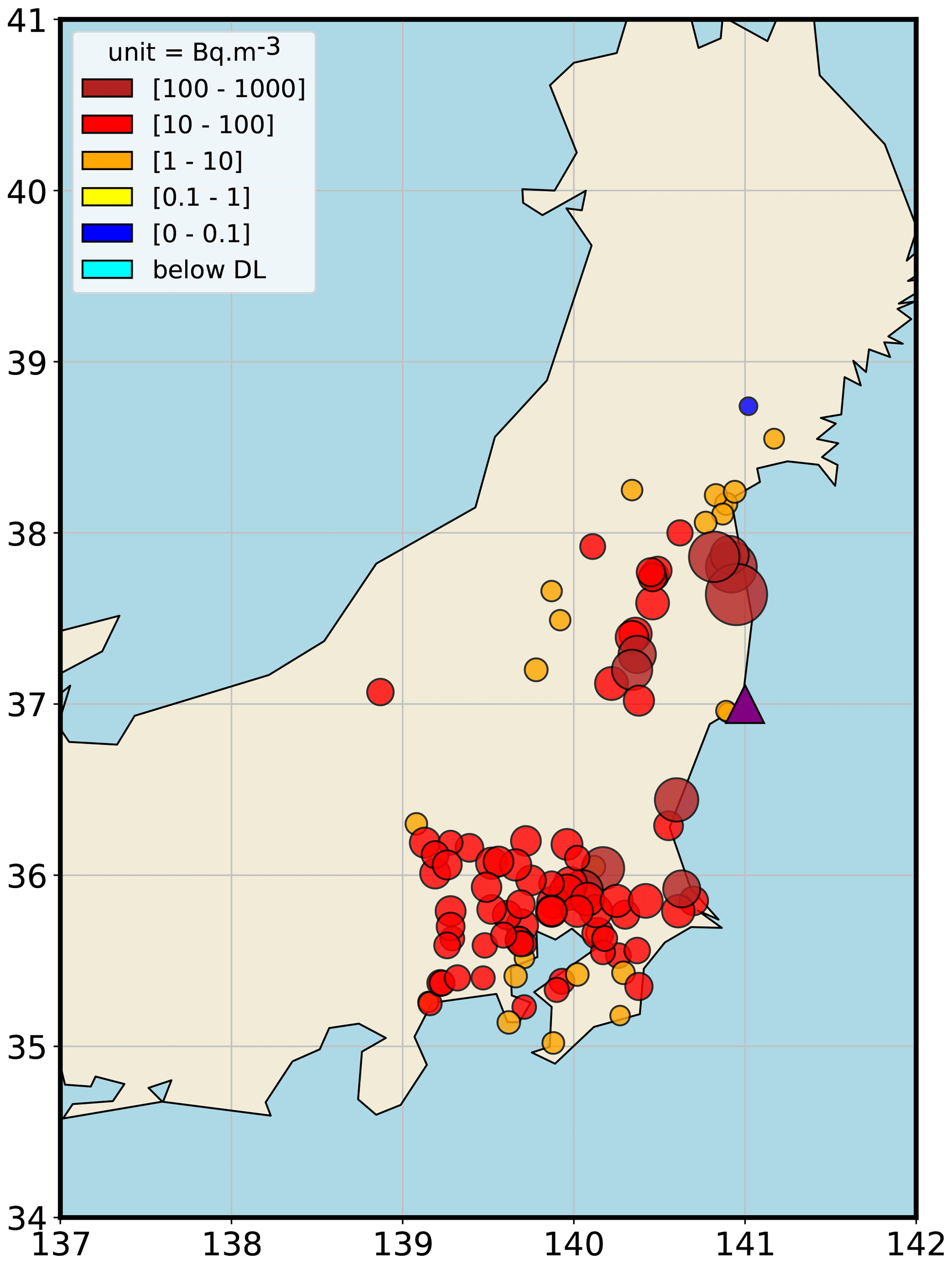
Figure 1Maximum air concentrations of 137Cs (in Bq m−3) measured in Japan in March 2011. The light blue points correspond to concentrations below the detection limit. The purple triangle corresponds to the Fukushima Daiichi NPP.
This allows us to better evaluate the relevance of our methods and to accurately estimate the uncertainties in the problem. Moreover, the majority of these observations are hourly, which allows for fine sampling of the 137Cs source term. Additionally, 1507 deposition measurements are used. This dataset is described and made available in MEXT (2012). The observations are located within 300 km of the Fukushima Daiichi NPP; however, measurements too close to the Fukushima Daiichi plant (typically less than 5 times the spatial resolution of the meteorological fields described in Table 1) are not used to consider the short-range dilution effects of the transport model. These measurements represent the averages of each grid cell of a field of deposition observations (in Bq m−2) measured by aerial radiation monitoring.
2.2 Physical parametrization
The atmospheric 137Cs plume dispersion is simulated with the Eulerian model ldX, which has already been validated on the Chernobyl and Fukushima Daiichi accidents (Quélo et al., 2007; Saunier et al., 2013) as well as on the 106Ru releases in 2017 (Saunier et al., 2019; Dumont Le Brazidec et al., 2020, 2021). The meteorological data used are the 3-hourly high-resolution forecast fields provided by the European Centre for Medium-Range Weather Forecasts (ECMWF) (see Table 1).
(Louis, 1979)(Troen and Mahrt, 1986)(Baklanov and Sørensen, 2001; Querel et al., 2021)Table 1Main set-up parameterizations of the ldX 137Cs transport simulations. The spatial and temporal resolutions are those of the ECMWF meteorological fields and the transport model. The other entries correspond to parameters of the transport model only.

The radionuclides, in particular 137Cs, were mainly deposited in the Fukushima Prefecture, north-west of the Fukushima Daiichi NPP. The bulk of the releases occurred over a 2-week period beginning on 11 March. Therefore, the model simulations start on 11 March 2011 at 00:00 UTC and end on 24 March 2011, corresponding to 312 h during which radionuclides could have been released. The release is assumed to be spread over the first two vertical layers of the model (between 0 and 160 m). The height of the release has a small impact, as the modelled predictions are compared with observations sufficiently far away from the Fukushima Daiichi NPP and the release mostly remains within the atmospheric boundary layer. Finally, it is assumed that all parameters describing the source aside from the reconstructed ones are known. This is, for instance, the case for the release height.
3.1 Reversible-jump MCMC
In this section, we describe the Bayesian reversible-jump MCMC algorithm used in the following to reconstruct the vector q discretized over a variable adaptive grid. A good description of the RJ-MCMC, which was introduced by Green (1995), can be found in Hastie and Green (2012). The algorithm is also clearly explained and applied by Bodin and Sambridge (2009). In particular, the method was used by Yee (2008) in the field of inverse modelling for the assessment of substance releases as well as by Liu et al. (2017) to quantify Fukushima Daiichi releases, although with a fixed number of variable-sized grid cells. A key asset of the RJ-MCMC technique is its ability to sample a highly variable release by balancing bias and variance errors.
The RJ-MCMC algorithm is a natural extension of the traditional Metropolis–Hastings (MH) algorithm to transdimensional discretization grids. In a traditional MH, the distribution of the release is assessed via a succession of random walks (e.g. Dumont Le Brazidec et al., 2020). In particular, special random walks allow the pdf of the discretization steps within the control vector x to be sampled.
Indeed, as described above, the function that describes the evolution of the release rate over time is a vector or step function, where each step (i.e. a grid cell) defines a constant release rate over a time interval. When using the RJ-MCMC, these time intervals are neither fixed nor regularly spaced. Hence, an objective is to retrieve the best stepwise time partition of the source term, which defines the release rates.
To do this, we use the concept of boundary: a boundary is a time that separates two constant release rates (i.e. that separates two grid cells where the source term is defined).
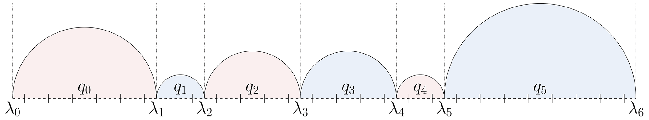
Figure 2Example of a source term partition: ) is the set of boundaries, and is the vector of release rates. The release rate defined on the time interval [λ2,λ3] is constant and equal to q2.
Let Λ be the set of Nb boundaries. Boundaries are 0, 312, and integers in (0 and 312 are natural and fixed boundaries), i.e. the boundaries are a selection among the hours of the release. Finding the probability distribution of the time steps associated with q is equivalent to finding the probability distribution of Λ. To retrieve the best discretizations of q, we can therefore sample Λ. Figure 2 presents an example of a source term partition.
The RJ-MCMC is basically equivalent to an MH algorithm except that some iterations of the algorithm are not intra-model random jumps (i.e. at constant Λ) but rather possibly inter-model random jumps (i.e. at non-constant Λ) or transdimensional (i.e. non-constant Λ size).
Specifically, we use three types of random jumps that govern the positions and number of boundaries: birth, death, and move. For these three processes, we draw on the work of Green (1995), Hastie and Green (2012), Liu et al. (2017), and (importantly) Bodin and Sambridge (2009). The birth process is the creation of a new boundary not yet present in , the death process is the removal of an existing boundary in Λ, and the move process is the displacement of an existing boundary in Λ. These processes must respect the detailed balance criterion in order to ensure the convergence of the Markov chain to the target distribution (Robert et al., 2018).
3.2 Handling observations and their errors
3.2.1 Measurements fusion
In this subsection, we propose a method to factor both concentration and deposition measurements into a Bayesian sampling by simply taking their disparity in the observation error matrix R into account. First of all, R is diagonal and is, therefore, described by a collection of scale parameters. Specifically, two scale parameters, rc and rd, are used when modelling R and are associated with the air concentration and deposition measurements respectively. Thus we can write the following:
where diag({ri}i) is the diagonal matrix of diagonal entries {ri}i. Note that we use the sorting algorithm described by Dumont Le Brazidec et al. (2021), which is applied to both the air concentration and deposition measurements, in all subsequent applications. This algorithm assigns a different scale parameter rnp to certain non-pertinent observations to prevent them from artificially reducing rc and rd. With this definition of R, the scale variables rc,rd, and rnp are included in the source vector x and, therefore, sampled using a MCMC.
3.2.2 Spatio-temporal observation error scale matrix modelling
In this subsection, we propose modelling R using the spatio-temporal information of the concentration observations. We assume that the error scale parameter corresponding to an observation–prediction pair depends mainly on the error in the model predictions. We also propose considering a prediction (i.e. an estimation of the number of radionuclides present at a definite time and place) as a point in a radionuclide plume at a specific time. The prediction modelling error varies according to its spatio-temporal position. Spatially, if two points of interest are distant by Δx, the difference in the errors in their attached model prediction is empirically assumed to be proportional to Δx. Temporally, let us consider two points in a plume with coordinates x1,x2 at times t and t+Δt respectively, where x1 and x2 are the longitude and latitude. These two points are moving with the plume, and they are spatially distant by v×Δt at time t, where v is a reference wind speed, representing the average wind over the accidental period. Therefore, the difference in the modelling errors of these points is estimated to be proportional to . In that respect, for each concentration observation, yi can be associated with three coordinates:
where x1,i, x2,i are the coordinates (in km) of the observation, v is set equal to 12 km h−1, and ti and Δt,i are the starting time and the duration of the observation in hours respectively. This average wind speed value has not been extensively researched and is only used to estimate the potential of the method. A clustering algorithm such as the k-means algorithm can be applied to partition these three coordinates' observation characteristics into several groups. A scale parameter rc,i can then be assigned to each group. If the algorithm for sorting pertinent and non-pertinent observations is applied, this yields
where , and rnp are the scale parameters associated with the spatial or spatio-temporal clusters of air concentration observations, the deposition measurements, and the non-pertinent observations respectively. The case where only the spatial qualification of the observation is used instead of both the spatial and temporal qualification is also addressed in this study.
In this section, we apply the previously introduced methods to the reconstruction of the Fukushima Daiichi 137Cs source term between 11 and 24 March. However, we first define the key statistical assumptions and parameters of the inversion set-up.
4.1 Statistical parametrization
The prior distributions determining the posterior distribution and the transition probabilities of the RJ-MCMC algorithm are defined in the next two sections.
4.1.1 Definition of the prior density functions
In this section, we specify the prior distributions of the source vector components: release rates and hyperparameters. The source release rate logarithms are assumed to follow a folded Gaussian prior distribution, so as to concurrently constrain the number of boundaries and the magnitude of the release rates. In the general case with Nimp=312, the scale matrix B of the folded Gaussian prior is defined as a 312×312 diagonal matrix. The entry bk of B is associated with the kth hour in , comprising hours where we consider the release of 137Cs possible. This yields the following:
where the folding position is defined as equal to the location term ln qb. We divide the 312 time intervals into two groups. The first “unconstrained” group consists of the time intervals during which we have noticed that a radionuclide emission does not trigger any noticeable observation. In other words, it is a time interval during which we have no information on a potential release. The unconstrained time intervals are the first 17 h of 11 March (hours in ), the days of 16 and 17 March (hours in ), and the last 18 h of 23 March (hours in ). The second group consists of the constrained time intervals. Two hyperparameters – bc for the constrained time intervals and bnc for the unconstrained time intervals – are used to describe the matrix B. If, instead of two, a single hyperparameter b is used for all release rates, the unconstrained time intervals are neither regularized by the observations nor by the prior. Indeed, to account for high release rates, samples of the distribution of b reach significant values. Low-magnitude release rates are then constrained very little by the corresponding prior. Release rates that are neither constrained by the observations nor by the priors can, in turn, reach very large values. This phenomenon was put forward by Liu et al. (2017). The mean of the folded Gaussian prior is chosen as ln qb=0 in order to regularize the unconstrained intervals. It is important to note that a release rate ln qi sampled by the RJ-MCMC is an aggregate of these hourly release rates, with each of them associated with either bc or bnc. Hence, we define the scale of the prior associated with the release rate ln qi defined between times ti and ti+kiΔt as follows:
where Bj,j is the jth diagonal coefficient of B, nc,i is the portion of constrained time intervals in kiΔt, and and wnc,i are the weighted numbers of the respective constrained and unconstrained hourly release rates included in the release rate ln qi. This definition is reflected in the prior cost:
where is the number of time steps (Nb being the number of boundaries) considered at a certain iteration by the RJ-MCMC and which characterizes the grid on which ln q is defined. The prior scale parameter bc is included in the source vector x and sampled with the rest of the variables. Such a prior on the release rate logarithms also has a constraining effect on the model's complexity (Occam's razor principle) through the normalization constant of the prior pdf.
An exponential prior distribution is used for the boundaries :
Here, . This prior has the effect of penalizing models that are too complex.
Furthermore, because no a priori information is available, the prior distributions on the coefficients of the observation error scale matrix are assumed to be uniform, and the prior values on the regularization scale terms are assumed to follow Jeffreys' prior distribution (Jeffreys, 1946; Liu et al., 2017). The lower and upper bounds of the uniform prior on the coefficients of the observation error matrix are set as zero and a large value, the latter of which is not necessarily realistic, as in Dumont Le Brazidec et al. (2021).
4.1.2 Parameters of the MCMC algorithm
In the Markov chain, the variables describing the source x are initialized randomly. The intra-model (i.e. with a fixed boundary partition) transitions defining the stochastic walks are set independently for each variable. Each transition probability is defined as a folded normal distribution, following Dumont Le Brazidec et al. (2020). Locations of the transition probabilities are the values of the variables at the current step. Variances of the related normal distribution are initialized at σln q=0.3 and σr=0.01, with the values being chosen by means of experiments. However, the value of σr is adaptive and is updated every 1000 iterations according to the predictions' values. Furthermore, the value of σr is not uniform across groups of observations: there are as many variances as observation clusters.
The algorithm runs initially as a classic MH for 104 iterations (only intra-model walks are allowed at this stage). Indeed, allowing transdimensional walks at the beginning of the run sometimes cause Markov chains to get stuck in local minima. In total, 2×10⁶ iterations are used; this large number ensures algorithm convergence (i.e. sufficient sampling of the posterior distribution of x) and corresponds to approximately 1 d of calculation for a 12-core computer. The burn-in is set to 106 iterations.
The inter-model transdimensional walks (with changing boundaries) are described in Appendix A, as they are technical. For this transdimensional case, uln q is the same for birth and death processes and is equal to 0.3. There is no variance parameter for the move walk. The probability of proposing an intra-model transition, a birth transition, a death transition and a move transition is , , , and respectively.
4.2 Results
To evaluate the quality of our reconstructed source term as well as the impact of the techniques proposed in Sect. 3, the distributions of the 137Cs source are sampled and compared using several settings:
-
Sect. 4.2.1 provides an activity-concentration-based reconstruction of the 137Cs source with a log-Cauchy likelihood and a threshold (to ensure it is defined for zero observations or predictions) of 0.5 Bq m−3 (Dumont Le Brazidec et al., 2021), the application of the observation sorting algorithm, and a spatial representation of R with 10 parameters. The vector
is sampled. A log-Cauchy likelihood is chosen because the associated reconstruction produces the best model-to-data comparisons among diverse choices of likelihoods and representations of R. The sampled source is compared to the source terms of Saunier et al. (2013) and Terada et al. (2020), and all variable marginal distributions are described.
-
In Sect. 4.2.2, we are interested in quantifying the impact of the addition of deposition measurements in the sampling with the method presented in Sect. 3.2.1. The source term is sampled in two configurations, namely with or without the addition of deposition measurements. That is, the vector
is sampled with or without rd. A threshold of 0.5 Bq m−2 is chosen for the deposition measurements.
-
Finally, we draw a selection of violin plots in Sect. 4.2.3 to assess the impact of the distribution of the observations in space and time clusters using the approach introduced in Sect. 3.2.2. More precisely, the fit to the observations of the reconstructed source is evaluated given the type of clustering (spatial or spatio-temporal) and the number of clusters.
4.2.1 Best reconstruction and comparison to other source terms
In this section, we provide the most appropriate reconstruction of the source term, based on the activity concentration measurements, from several choices of likelihoods and R representations. This best reconstruction is chosen with the help of a model-to-data comparison, i.e. FAC (factor) scores, representing the proportion of measurements for which the observed and modelled values agree. The chosen likelihood is a log-Cauchy distribution with a threshold of 0.5 Bq m−3, and air concentration measurements are spatially clustered in nine groups using the k-means method.
Figure 3 shows the temporal evolution of the median release rate with its associated standard deviation (i.e. the evolution of the hourly release rates samples that are obtained from the Nimp RJ-MCMC samples). This temporal evolution is compared to the source term from Saunier et al. (2013), which was estimated from gamma dose rate measurements but from the same meteorological data and transport model, and to the more recent source term from Terada et al. (2020).
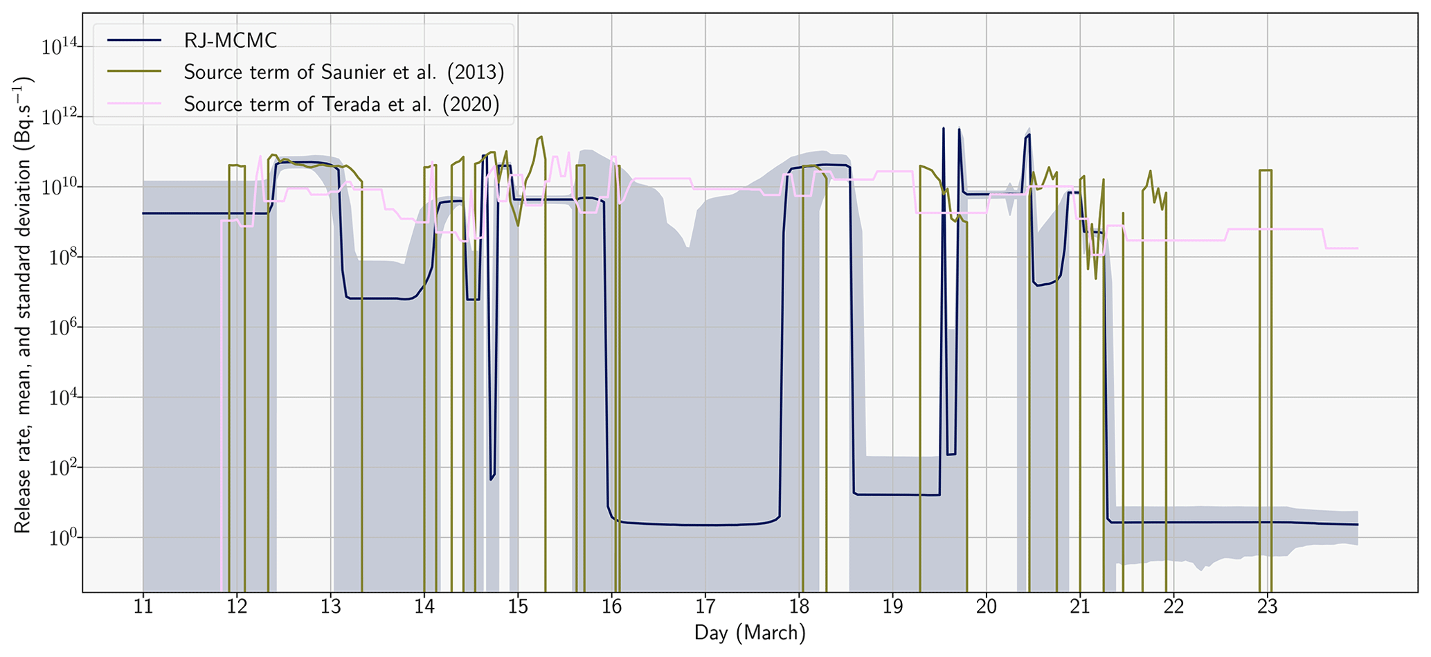
Figure 3Evolution of the release rate (in Bq s−1) describing the 137Cs source (UTC) sampled with the RJ-MCMC algorithm. The blue line corresponds to the sampled median release rate. The light blue area corresponds to the area between μln q, the median, and σln q, the standard deviation, of the reconstructed hourly release rates: . Our source term is compared to the source terms of Saunier et al. (2013) and Terada et al. (2020).
Firstly, we observe that a good match is obtained between the median release and the source term of Saunier et al. (2013) or Terada et al. (2020) (on the constrained time intervals), as the differences between releases under 109 Bq s−1 can be neglected. Indeed, between the 11 and the 19 March 2011, the three source terms have similar peak magnitudes (close to 1011 Bq s−1); these peaks are observed at neighbouring time intervals. Between the 19 and the 21 March, a notable difference can be observed: the RJ-MCMC source term predicts very high 1 h peaks (close to 1012 Bq s−1), whereas the Terada et al. (2020) source term distributes the release uniformly over the whole period. Secondly, release rates are subject to large variations. Indeed, there are periods of important temporal variability in the release rate (e.g. between 19 and 21 March) and of low temporal variability (e.g. between 11 and 14 March). This justifies the use of the RJ-MCMC transdimensional algorithm, as it allows one to reconstruct certain time intervals of the release with a greater accuracy and others with less complexity. Thirdly, the temporal evolution of the release can be explored, and several prominent peaks can be observed with a magnitude approaching or surpassing 1011 Bq s−1: between 12 and 14 March, between 14 and 16 March, on 18 March, and between 19 and 21 March.
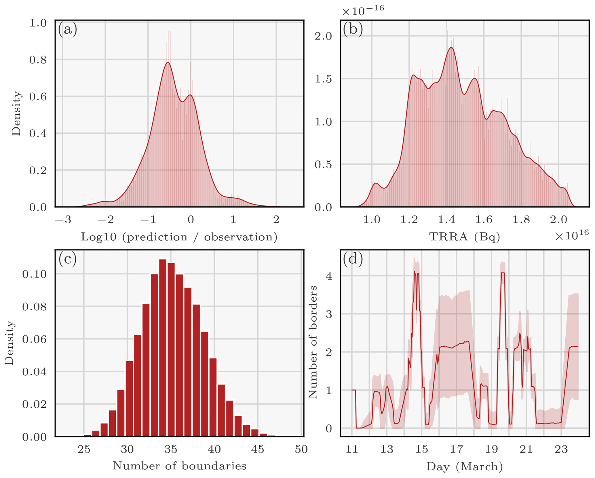
Figure 4Densities or averages of variables describing the 137Cs source reconstructed with the RJ-MCMC technique: (a) density of relative differences in log10 between observations and predictions; (b) density of the total retrieved released activity (TRRA) of 137Cs during the Fukushima Daiichi accident (in Bq) – outliers are removed; (c) histogram of the number of boundaries; and (d) mean (± standard deviation) of the number of boundaries as a function of time (UTC).
Figure 4a describes the histogram of relative differences in log10 between predictions (medians of the predictions computed using the samples are employed) and air concentration observations larger than 0.5 Bq m−3. A value of −1, therefore, corresponds to an observation 10 times larger than a prediction. A good fit between observations and predictions can be observed, although the observations are globally underestimated by the predictions.
Figure 4b shows the pdf of the total release (in Bq). It can be seen from this density that most of the total release distribution mass is sampled between 10 and 20 PBq and peaks at 14 PBq. This is consistent with previous studies which estimate the release to be between 5 and 30 PBq (Chino et al., 2011; Terada et al., 2012; Winiarek et al., 2012, 2014; Saunier et al., 2013; Katata et al., 2015; IAEA, 2015; Yumimoto et al., 2016; Liu et al., 2017; Terada et al., 2020). However, note that these works attempted to estimate potential releases beyond 24 March.
Figure 4c plots the pdf of the number of boundaries (i.e. a measure of model complexity) sampled by the algorithm. Here, the minimum of the distribution is 25 boundaries and the maximum is 45 with a peak at 35 boundaries. Recall that the maximum number of boundaries is 313.
Figure 4d shows the average number of sampled boundaries at each time and the associated standard deviation. The y axis corresponds to the number of boundaries counted: for a given hour t, we draw
i.e. the average over all samples of the number of boundaries counted around t. In essence, the curve shows the number of boundaries necessary to model the release at a certain time (i.e. the variability in the release according to the algorithm). We observe that there is a large variability between 14 and 15 March as well as between 19 and 21 March. This correlates very well with the observable results in Fig. 3. This observation once again confirms the relevance of using the RJ-MCMC algorithm: periods of high variability can be sampled finely.
4.2.2 Impact of using deposition measurements
In this section, we study the impact of adding 1507 deposition measurements to the 14 248 air concentration measurements. A log-Cauchy distribution with a threshold of 0.5 Bq m−3 for the air concentration measurements and 0.5 Bq m−2 for the deposit measurements is employed. Air concentration measurements are clustered with a spatial k-means algorithm in nine groups, as described in Sect. 4.2.1. To quantify the impact of the added measurements, we sample the following vector with an RJ-MCMC algorithm in two cases, with or without deposition measurements, i.e. with or without rd, as follows:
In the case without deposition measurements, we use the same samples as in Sect. 4.2.1. A posteriori marginals of these control variables are displayed in Fig. 5.
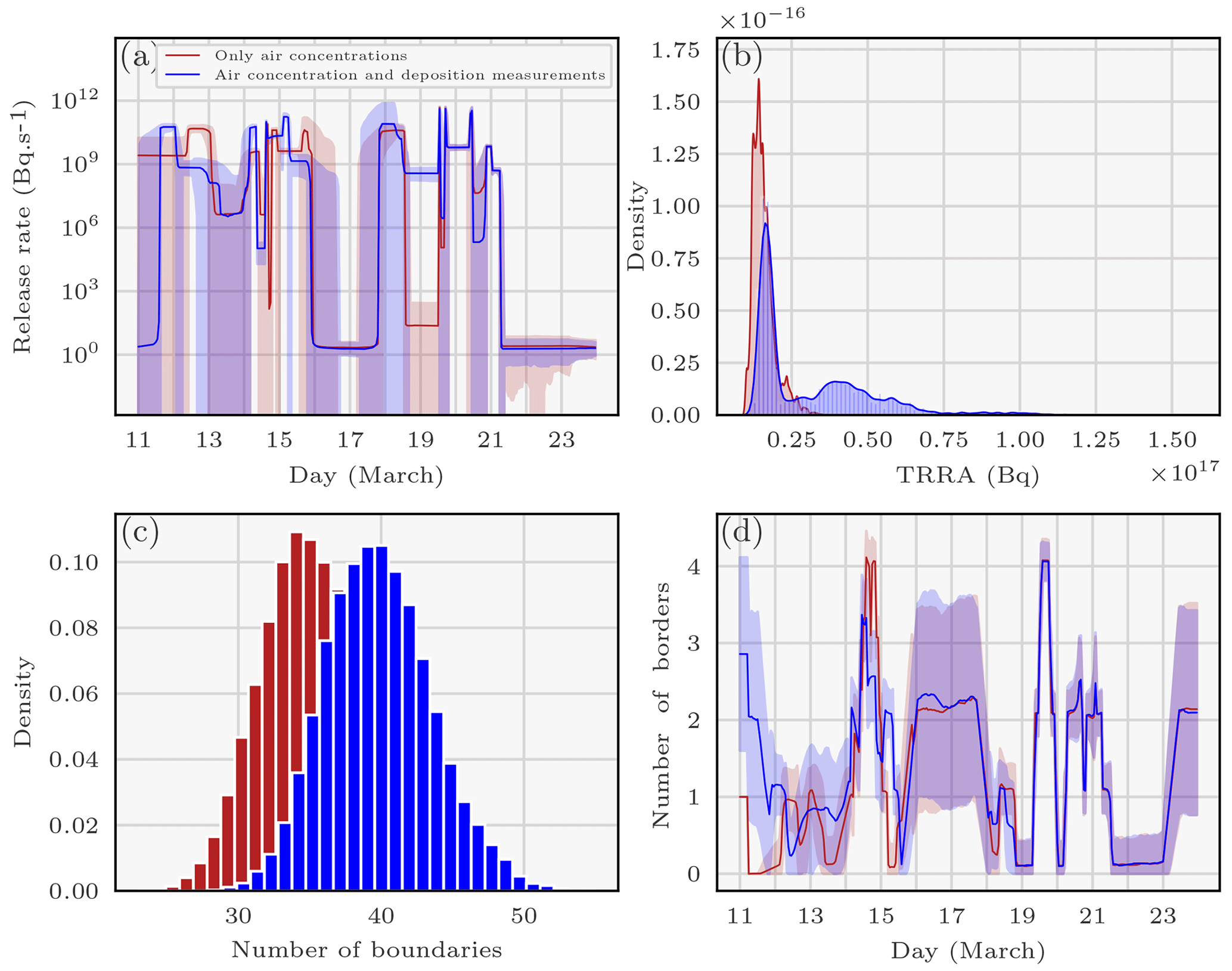
Figure 5The panels correspond to probability densities or averages of variables describing the 137Cs source reconstructed with the RJ-MCMC technique using air concentration and deposition measurements. Panel (a) displays the medians and standard deviations of hourly release rates. The red and blue curves correspond to the sampled median release rates. The red and light blue areas correspond to the areas between μln q, the median, and σln q, the standard deviation, of the sampled hourly release rates for each reconstruction: . Panel (b) shows the probability density of the total release of 137Cs during the Fukushima Daiichi accident (in Bq). Panel (c) provides a histogram of the number of boundaries. Panel (d) shows the mean (± standard deviation) of the number of boundaries according to the hour considered.
In Fig. 5a, the medians of the two sampling datasets are similar, except for the release rates between 11 and 14 March. Indeed, when using air concentration and deposition measurements, the release rate peaks on 12 March instead of on 13 March, the latter of which is the case when using air concentrations alone.
In Fig. 5b, the main mode of the total retrieved released activity (TRRA) distribution retrieved using the air concentration and deposition measurements is 5 PBq larger than the TRRA reconstructed with the air concentration measurements alone. Moreover, the reconstructed density with both types of measurements has a large variance and leads to the possibility of a larger release (up to 75 PBq). The density of the number of boundaries with both types of measurements is shifted to higher values compared with the density with air concentrations alone, which indicates a reconstructed release of greater complexity (Fig. 5c). This is consistent with the fact that the second release is reconstructed with a larger number of observations.
In Fig. 5d, the number of boundaries was estimated to be half as large on 14 March when deposition measurements were used, but it was estimated to be larger on 15 March. These differences are rather surprising insofar as there is no obvious disparity between the medians of the release rates for the two reconstructions in Fig. 5a on these days.
In Table 2, we evaluate the FAC 2, FAC 5, and FAC 10 scores for both cases. FAC scores are common metrics for measuring the fit of a source term with available observations. The FAC 2, FAC 5, and FAC 10 are the proportion of measurements for which the observed and modelled values agree by a factor of 2, 5, or 10 respectively. For example, a FAC 2 score of 0.32 with respect to the air concentration measurements means that 32 % of the predictions (i.e. simulated measurements) are such that
where Nobs is the number of observations considered, and yt is a threshold set at 0.5 Bq m−3. This threshold is added to limit the weight of low values, considered of lesser interest, in the indicator. Finally, to calculate the FAC scores, only observations above 1 Bq m−3 are considered.
Saunier et al. (2013)Terada et al. (2020)Table 2Comparison of observed and simulated measurements from reconstructed predictions with air concentration measurements only or with air concentration and deposition measurements. The FAC 2, FAC 5, and FAC 10 are the proportion of measurements for which the observed and modelled values agree by a factor of 2, 5, or 10 respectively. For example, the table reads as follows: the predictions calculated based on air concentrations only obtain a FAC 5 score of 0.58 with respect to the deposition measurements.
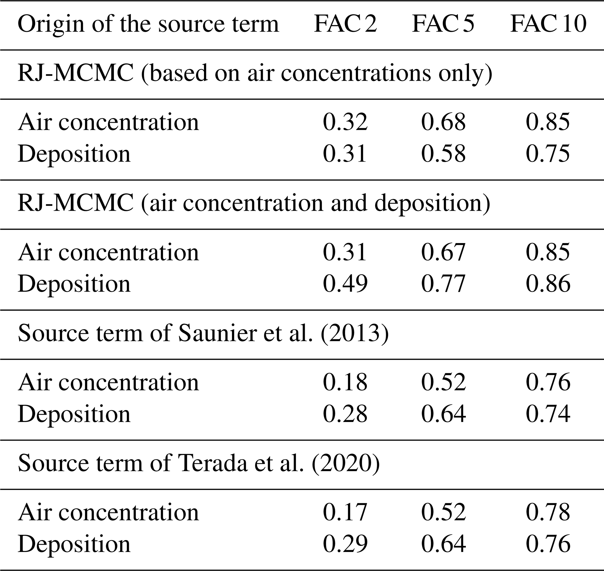
The FAC scores show that the source term obtained with the RJ-MCMC has a better agreement with the air concentration measurements than the Saunier et al. (2013) or Terada et al. (2020) source terms. This shows that the RJ-MCMC is able to sample source terms consistent with air concentration measurements but does not allow us to reach a conclusion regarding its performance: the sampling algorithm was optimized using air concentrations, whereas, for example, the Saunier et al. (2013) source term was recovered from dose rate measurements. However, the source term found with the RJ-MCMC on air concentration measurements can be fairly evaluated using deposition measurements. It is observed that the fits with the deposition measurements of the three source terms are similar.
Furthermore, as expected, Table 2 shows that there is a significant difference in the fit with the deposition measurements when they are added to the observation dataset used to reconstruct the source term. However, the addition of the deposition measurements has no impact on the quality of the fit to the air concentration measurements. This suggests that an RJ-MCMC optimized on dose rate measurements, in addition to the deposition and air concentrations, may obtain a good agreement with the dose rate measurements, without degrading its results on deposition or air concentrations.
4.2.3 Impact of the observation error matrix R representation
In this section, we investigate the spatial and spatio-temporal representation of the R likelihood scale matrix. Figure 6 presents violin plots of the FAC 2 and FAC 5 scores for air concentration measurements against the number of scale parameters chosen to describe R (i.e. the number of observations clusters). Violin plots are created out of the best scores of 44 RJ-MCMC sampling datasets with diverse likelihoods chosen after Dumont Le Brazidec et al. (2021) in order to make the conclusions less dependent on statistical modelling. The chosen numbers of spatial clusters (1, 2, and 9) and spatio-temporal clusters (3 and 7) of the violins are a selection for the sake of clarity.
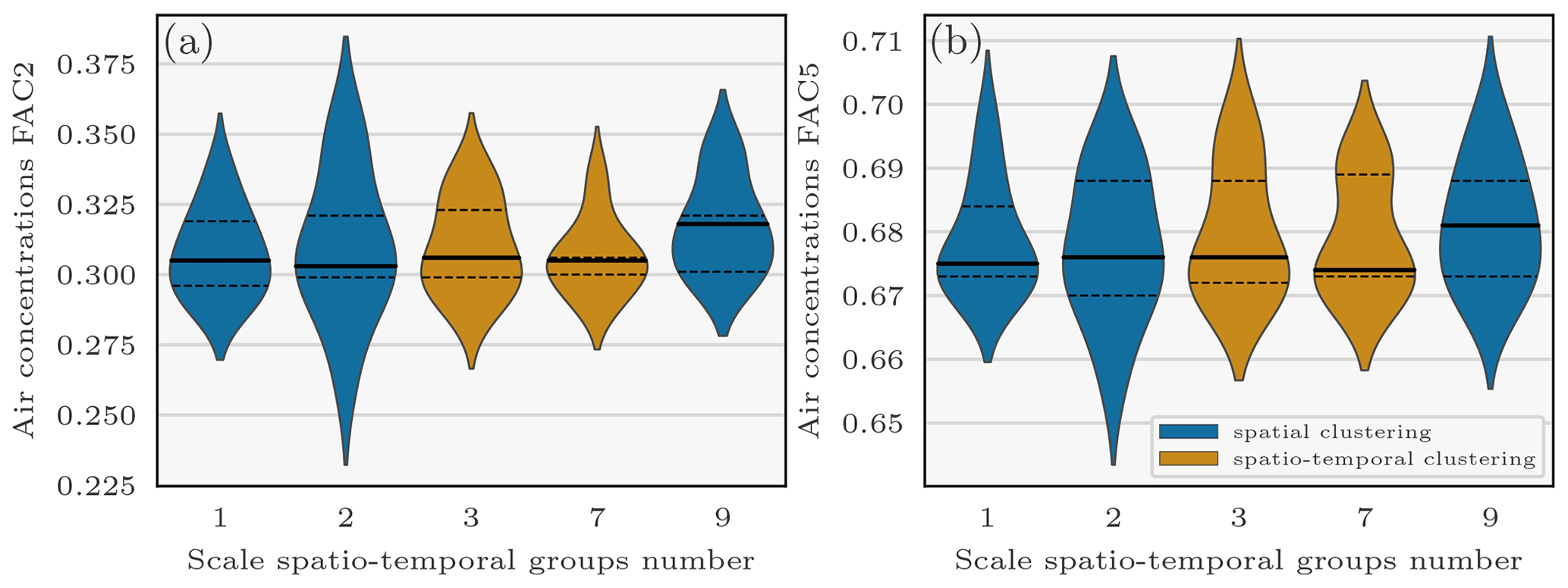
Figure 6Violin plots of the air concentration FAC 2 and FAC 5 scores against the observation error scale parameters' spatio-temporal groups number. Points composing the violin plots consist of the best FAC 2 and FAC 5 scores of 44 sampling datasets using diverse configurations of likelihoods and thresholds (log-normal, log-Laplace, and log-Cauchy) chosen according to Dumont Le Brazidec et al. (2021). The horizontal segments within the violins represent (from bottom to top) the respective first, second, and third quartiles. The chosen numbers of spatial and spatio-temporal clusters are only a selection for the sake of clarity.
For both the FAC 2 and FAC 5 air concentration scores, it can be observed that the spatio-temporal labelling of the observations does not increase the quality of the scores, whereas the number of spatial clusters does. For example, we can observe a difference of 0.02 between the second quartile of the FAC 2 score for sampling datasets with two spatial groups and the second quartile of the FAC 2 score for sampling datasets with nine spatial groups. One hypothesis is that the error is mainly related to the distance to the source and remains relatively homogeneous in time. However, the use of an accurate estimate of the effective wind speed as a function of time and depending on the position of the observations is necessary to draw conclusions; such a study is outside the scope of this paper.
In this paper, we investigated a transdimensional sampling method to reconstruct highly fluctuating radionuclide atmospheric sources and applied it to assess the 137Cs Fukushima Daiichi release. Furthermore, we proposed two more methods to add information to the model in order to reduce uncertainties attached to such a complex release.
Firstly, an RJ-MCMC algorithm was defined. This MH extension to transdimensional meshes allows one to sample both the source term and its underlying adaptive discretization in time. In the case of complex releases, an adaptive grid allows one to reconstruct the source term with high accuracy and discretization consistent with the available observations.
Secondly, we have focused on ways to add information by adapting the representation of the observation error matrix R. We proposed the assimilation of deposition measurements or spatial and temporal information on the air concentration observations by increasing the complexity of R.
Subsequently, the distributions of the variables defining the source of 137Cs were fully sampled. This enabled the estimation of the uncertainties associated with these variables as well as the evaluation and demonstration of the merits of the methods.
Firstly, we observed that the predictions reproduce the air concentration and deposition observations well. When using air concentrations only, the FAC 2 and FAC 5 scores corresponding to air concentration measurements are 0.32 and 0.68 respectively. The main part of the best total release distribution mass is estimated to be between 10 and 20 PBq and peaks at 14 PBq, which is in accord with previous estimations.
Secondly, the periods of high variability in 137Cs releases have been reconstructed with accuracy by the RJ-MCMC algorithm. The transdimensional method also allowed the periods of low temporal variability to be sampled more coarsely, thereby avoiding variance errors and saving computing time, which, in particular, confirms the conclusions of Liu et al. (2017). The priors that we chose allowed for an efficient regularization of the release rates and their adaptive mesh.
Finally, the use of combined air concentration and deposition measurements had an impact on the reconstruction of the TRRA distribution, the mean of which increased by 10 PBq. The spatial clustering methods proved to increase the quality of the predictions by improving the model-to-data comparison.
We recommend the use of the RJ-MCMC for long-release source reconstruction. It allows one to sample highly variable source terms with great accuracy by solving the bias–variance trade-off. We also recommend the use of advanced modelling of R considering the deposition measurements and the spatial information of the air concentration observations which have proven to be valuable in reducing the observation–prediction discrepancies.
Here, we describe the mathematical details of the three inter-model walks: move, birth, and death. The move process is intra-dimensional. Provided that the move is a symmetric motion, the associated g-transition distribution is symmetric, i.e.
The birth process is the creation of a new boundary, a walk from xi (a vector composed of n boundaries) to xj (a vector composed of n+1 boundaries) is proposed. In other words, by generating a new boundary, one release rate is destroyed and two new release rates emerge from this destruction. We therefore assign two new release rates and , with uln q (a Gaussian noise). The transition probability is defined as follows (Bodin and Sambridge, 2009):
The probability of a birth at a certain position among positions not occupied by boundaries is
Furthermore, the probability of generating new release rates is Gaussian:
where the new boundary here is generated at hour k−1.
The probability of death of one among the Nimp−1 boundaries is
which is a uniform choice among Nimp−1 possibilities. On the other hand, the probability of destroying the release associated with this position is 1.
Each dataset used in the paper is available via a DOI on a compliant repository or directly in the cited papers. More precisely, the air concentration observation datasets used in the inversions are available in Oura et al. (2015) from http://www.radiochem.org/en/j-online152.html (last access: 3 February 2023) and in Tsuruta et al. (2018), Tanaka et al. (2013), Takehisa et al. (2012), and Yamada et al. (2013). In addition, the deposition observation dataset used in the inversions is available via https://doi.org/10.5281/zenodo.7016491 (Dumont Le Brazidec and Saunier, 2022). The IBISA (inverse Bayesian inference for source assessment) algorithm, which specifically describes the reversible-jump Markov chain Monte Carlo algorithm used in this article, is available from https://doi.org/10.5281/zenodo.7318543 (Dumont Le Brazidec et al., 2022).
JDLB: software, methodology, conceptualization, investigation, writing – original draft, and visualization. MB: methodology, software, conceptualization, writing – review and editing, visualization, and supervision. OS: resources, methodology, conceptualization, writing – review and editing, visualization, and supervision. YR: methodology, software, and writing – review and editing.
The contact author has declared that none of the authors has any competing interests.
Publisher’s note: Copernicus Publications remains neutral with regard to jurisdictional claims in published maps and institutional affiliations.
The authors would like to thank the European Centre for Medium-Range Weather Forecasts (ECMWF) for making available the meteorological fields used in this study. They would also like to thank Sophie Ricci, Lionel Soulhac, Paola Cinnella, Didier Lucor, Yann Richet, and Anne Mathieu for their suggestions and advice on this work. CEREA is a member of the Institut Pierre-Simon Laplace (IPSL).
This paper was edited by Dan Lu and reviewed by two anonymous referees.
Baklanov, A. and Sørensen, J. H.: Parameterisation of radionuclide deposition in atmospheric long-range transport modelling, Phys. Chem. Earth Pt. B, 26, 787–799, https://doi.org/10.1016/S1464-1909(01)00087-9, 2001. a
Bodin, T. and Sambridge, M.: Seismic tomography with the reversible jump algorithm, Geophys. J. Int., 178, 1411–1436, https://doi.org/10.1111/j.1365-246X.2009.04226.x, 2009. a, b, c, d
Chino, M., Nakayama, H., Nagai, H., Terada, H., Katata, G., and Yamazawa, H.: Preliminary Estimation of Release Amounts of 131I and 137Cs Accidentally Discharged from the Fukushima Daiichi Nuclear Power Plant into the Atmosphere, J. Nucl. Sci. Technol, 48, 1129–1134, https://doi.org/10.1080/18811248.2011.9711799, 2011. a, b
Delle Monache, L., Lundquist, J., Kosović, B., Johannesson, G., Dyer, K., Aines, R. D., Chow, F., Belles, R., Hanley, W., Larsen, S., Loosmore, G., Nitao, J., Sugiyama, G., and Vogt, P.: Bayesian inference and markov chain monte carlo sampling to reconstruct a contaminant source on a continental scale, J. Appl. Meteorol. Clim., 47, 2600–2613, https://doi.org/10.1175/2008JAMC1766.1, 2008. a, b
Dumont Le Brazidec, J. and Saunier, O.: Statistics on caesium 137 deposition around the Fukushima-Daiichi plant after the 2011 accident, Zenodo [data set], https://doi.org/10.5281/zenodo.7016491, 2022. a
Dumont Le Brazidec, J., Bocquet, M., Saunier, O., and Roustan, Y.: MCMC methods applied to the reconstruction of the autumn 2017 Ruthenium-106 atmospheric contamination source, Atmos. Environ., 6, 100071, https://doi.org/10.1016/j.aeaoa.2020.100071, 2020. a, b, c, d, e
Dumont Le Brazidec, J., Bocquet, M., Saunier, O., and Roustan, Y.: Quantification of uncertainties in the assessment of an atmospheric release source applied to the autumn 2017 106Ru event, Atmos. Chem. Phys., 21, 13247–13267, https://doi.org/10.5194/acp-21-13247-2021, 2021. a, b, c, d, e, f, g, h, i
Dumont Le Brazidec, J., Bocquet, M., Saunier, O., and Roustan, Y.: Inverse Bayesian Inference for Source Assesment (1.0.0), Zenodo [data set], https://doi.org/10.5281/zenodo.7318543, 2022. a
Furuta, S., Sumiya, S., Watanabe, H., Nakano, M., Imaizumi, K., Takeyasu, M., Nakada, A., Fujita, H., Mizutani, T., Morisawa, M., Kokubun, Y., Kono, T., Nagaoka, M., Yokoyama, H., Hokama, T., Isozaki, T., Nemoto, M., Hiyama, Y., Onuma, T., Kato, C., and Kurachi, T.: Results of the environmental radiation monitoring following the accident at the Fukushima Daiichi Nuclear Power Plant Interim report Ambient radiation dose rate, radioactivity concentration in the air and radioactivity concentration in the fallout, Tech. rep., Radiation Protection Department, Nuclear Fuel Cycle Engineering Laboratories, Tokai Research and Development Center, Japan Atomic Energy Agency, Japan, jAEA-Review–2011-035 INIS Reference Number: 43088311, OSTI ID: 21609259, 2011. a
Green, P. J.: Reversible jump Markov chain Monte Carlo computation and Bayesian model determination, Biometrika, 82, 711–732, https://doi.org/10.1093/biomet/82.4.711, 1995. a, b
Hastie, D. I. and Green, P. J.: Model choice using reversible jump Markov chain Monte Carlo, Stat. Neerl., 66, 309–338, https://doi.org/10.1111/j.1467-9574.2012.00516.x, 2012. a, b
Hastie, T., Tibshirani, R., and Friedman, J.: The Elements of Statistical Learning: Data Mining, Inference, and Prediction, Second Edition, Springer Series in Statistics, Springer-Verlag, New York, 2 edn., ISBN 978-0-387-84857-0, 2009. a
Hirao, S., Yamazawa, H., and Nagae, T.: Estimation of release rate of iodine-131 and cesium-137 from the Fukushima Daiichi nuclear power plant, J. Nucl. Sci. Technol., 50, 139–147, https://doi.org/10.1080/00223131.2013.757454, 2013. a
IAEA: The Fukushima Daiichi accident, Tech. rep., Vienna, 978-92-0-107015-9, 2015. a
Jeffreys, H.: An invariant form for the prior probability in estimation problems, P. Roy. Soc. Lond. A Mat., 186, 453–461, https://doi.org/10.1098/rspa.1946.0056, 1946. a
Katata, G., Ota, M., Terada, H., Chino, M., and Nagai, H.: Atmospheric discharge and dispersion of radionuclides during the Fukushima Dai-ichi Nuclear Power Plant accident. Part I: Source term estimation and local-scale atmospheric dispersion in early phase of the accident, J. Environ. Radioact., 109, 103–113, https://doi.org/10.1016/j.jenvrad.2012.02.006, 2012. a
Katata, G., Chino, M., Kobayashi, T., Terada, H., Ota, M., Nagai, H., Kajino, M., Draxler, R., Hort, M. C., Malo, A., Torii, T., and Sanada, Y.: Detailed source term estimation of the atmospheric release for the Fukushima Daiichi Nuclear Power Station accident by coupling simulations of an atmospheric dispersion model with an improved deposition scheme and oceanic dispersion model, Atmos. Chem. Phys., 15, 1029–1070, https://doi.org/10.5194/acp-15-1029-2015, 2015. a, b
Keats, A., Yee, E., and Lien, F.-S.: Bayesian inference for source determination with applications to a complex urban environment, Atmos. Environ., 41, 465–479, https://doi.org/10.1016/j.atmosenv.2006.08.044, 2007. a
Kobayashi, T., Nagai, H., Chino, M., and Kawamura, H.: Source term estimation of atmospheric release due to the Fukushima Dai-ichi Nuclear Power Plant accident by atmospheric and oceanic dispersion simulations, J. Nucl. Sci. Technol., 50, 255–264, https://doi.org/10.1080/00223131.2013.772449, 2013. a
Li, X., Sun, S., Hu, X., Huang, H., Li, H., Morino, Y., Wang, S., Yang, X., Shi, J., and Fang, S.: Source inversion of both long- and short-lived radionuclide releases from the Fukushima Daiichi nuclear accident using on-site gamma dose rates, J. Hazard. Mater., 379, 120770, https://doi.org/10.1016/j.jhazmat.2019.120770, 2019. a
Liu, Y., Haussaire, J.-M., Bocquet, M., Roustan, Y., Saunier, O., and Mathieu, A.: Uncertainty quantification of pollutant source retrieval: comparison of Bayesian methods with application to the Chernobyl and Fukushima Daiichi accidental releases of radionuclides, Q. J. Roy. Meteor. Soc., 143, 2886–2901, https://doi.org/10.1002/qj.3138, 2017. a, b, c, d, e, f, g, h, i, j, k, l
Louis, J.-F.: A parametric model of vertical eddy fluxes in the atmosphere, Bound.-Lay. Meteorol., 17, 187–202, https://doi.org/10.1007/BF00117978, 1979. a
Mathieu, A., Korsakissok, I., Quélo, D., Groëll, J., Tombette, M., Didier, D., Quentric, E., Saunier, O., Benoit, J.-P., and Isnard, O.: Atmospheric Dispersion and Deposition of Radionuclides from the Fukushima Daiichi Nuclear Power Plant Accident, Elements, 8, 195–200, https://doi.org/10.2113/gselements.8.3.195, 2012. a
MEXT: NRA: Results of the (i) Fifth Airborne Monitoring Survey and (ii) Airborne Monitoring Survey Outside 80 km from the Fukushima Dai-ichi NPP, http://radioactivity.nsr.go.jp/en/contents/6000/5790/24/203_0928_14e.pdf (last access: 3 February 2023), 2012. a
Nagai, H., Terada, H., Tsuduki, K., Katata, G., Ota, M., Furuno, A., and Akari, S.: Updating source term and atmospheric dispersion simulations for the dose reconstruction in Fukushima Daiichi Nuclear Power Station Accident, EPJ Web Conf., 153, 08012, https://doi.org/10.1051/epjconf/201715308012, 2017. a
Nagakawa, Y., Sotodate, T., Kinjo, Y., and Suzuki, T.: One-year time variations of anthropogenic radionuclides in aerosols in Tokyo after the Fukushima Dai-ichi Nuclear Power Plant reactor failures, J. Nucl. Sci. Technol., 52, 784–791, https://doi.org/10.1080/00223131.2014.985279, 2015. a
Oura, Y., Ebihara, M., Tsuruta, H., Nakajima, T., Ohara, T., Ishimoto, M., Sawahata, H., Katsumura, Y., and Nitta, W.: A Database of Hourly Atmospheric Concentrations of Radiocesium (134Cs and 137Cs) in Suspended Particulate Matter Collected in March 2011 at 99 Air Pollution Monitoring Stations in Eastern Japan, J. Nucl. Radiochem. Sci., 15, 2_1–2_12, https://doi.org/10.14494/jnrs.15.2_1, 2015 (data available at: http://www.radiochem.org/en/j-online152.html, last access: 3 February 2023). a, b
Querel, A., Quelo, D., Roustan, Y., and Mathieu, A.: Sensitivity study to select the wet deposition scheme in an operational atmospheric transport model, J. Environ. Radioactiv., 237, 106712, https://doi.org/10.1016/j.jenvrad.2021.106712, 2021. a
Quélo, D., Krysta, M., Bocquet, M., Isnard, O., Minier, Y., and Sportisse, B.: Validation of the Polyphemus platform on the ETEX, Chernobyl and Algeciras cases, Atmos. Environ., 41, 5300–5315, https://doi.org/10.1016/j.atmosenv.2007.02.035, 2007. a
Robert, C. P., Elvira, V., Tawn, N., and Wu, C.: Accelerating MCMC algorithms, Wiley Interdiscip. Rev. Comput. Stat., 10, e1435, https://doi.org/10.1002/wics.1435, 2018. a
Saunier, O., Mathieu, A., Didier, D., Tombette, M., Quélo, D., Winiarek, V., and Bocquet, M.: An inverse modeling method to assess the source term of the Fukushima Nuclear Power Plant accident using gamma dose rate observations, Atmos. Chem. Phys., 13, 11403–11421, https://doi.org/10.5194/acp-13-11403-2013, 2013. a, b, c, d, e, f, g, h, i, j
Saunier, O., Didier, D., Mathieu, A., Masson, O., and Dumont Le Brazidec, J.: Atmospheric modeling and source reconstruction of radioactive ruthenium from an undeclared major release in 2017, P. Natl. Acad. Sci. USA, 116, 24991–25000, https://doi.org/10.1073/pnas.1907823116, 2019. a
Stohl, A., Seibert, P., Wotawa, G., Arnold, D., Burkhart, J. F., Eckhardt, S., Tapia, C., Vargas, A., and Yasunari, T. J.: Xenon-133 and caesium-137 releases into the atmosphere from the Fukushima Dai-ichi nuclear power plant: determination of the source term, atmospheric dispersion, and deposition, Atmos. Chem. Phys., 12, 2313–2343, https://doi.org/10.5194/acp-12-2313-2012, 2012. a
Takehisa, O., Tetsuya, O., Mitsumasa, T., Yukio, S., Masamitsu, K., Hitoshi, A., Yasuaki, K., Masatsugu, K., Jun, S., Masahiro, T., Hitoshi, O., Shunsuke, T., Shunsuke, T., Tadahiro, S., and Tadahiro, S.: Emergency Monitoring of Environmental Radiation and Atmospheric Radionuclides at Nuclear Science Research Institute, JAEA Following the Accident of Fukushima Daiichi Nuclear Power Plant, JAEA-Data, https://jglobal.jst.go.jp/en/detail?JGLOBAL_ID=201402276577269847 (last access: 3 Februaru 2023), 2012. a, b
Tanaka, K., Sakaguchi, A., Kanai, Y., Tsuruta, H., Shinohara, A., and Takahashi, Y.: Heterogeneous distribution of radiocesium in aerosols, soil and particulate matters emitted by the Fukushima Daiichi Nuclear Power Plant accident: retention of micro-scale heterogeneity during the migration of radiocesium from the air into ground and river systems, J. Radioanal. Nucl. Ch., 295, 1927–1937, https://doi.org/10.1007/s10967-012-2160-9, 2013. a, b
Terada, H., Katata, G., Chino, M., and Nagai, H.: Atmospheric discharge and dispersion of radionuclides during the Fukushima Dai-ichi Nuclear Power Plant accident. Part II: verification of the source term and analysis of regional-scale atmospheric dispersion, J. Environ. Radioact., 112, 141–154, https://doi.org/10.1016/j.jenvrad.2012.05.023, 2012. a, b
Terada, H., Nagai, H., Tsuduki, K., Furuno, A., Kadowaki, M., and Kakefuda, T.: Refinement of source term and atmospheric dispersion simulations of radionuclides during the Fukushima Daiichi Nuclear Power Station accident, J. Environ. Radioact., 213, 106104, https://doi.org/10.1016/j.jenvrad.2019.106104, 2020. a, b, c, d, e, f, g, h, i
Tichý, O., Šmídl, V., Hofman, R., and Stohl, A.: LS-APC v1.0: a tuning-free method for the linear inverse problem and its application to source-term determination, Geosci. Model Dev., 9, 4297–4311, https://doi.org/10.5194/gmd-9-4297-2016, 2016. a
Troen, I. B. and Mahrt, L.: A simple model of the atmospheric boundary layer; sensitivity to surface evaporation, Bound.-Lay. Meteorol., 37, 129–148, https://doi.org/10.1007/BF00122760, 1986. a
Tsuruta, H., Oura, Y., Ebihara, M., Moriguchi, Y., Ohara, T., and Nakajima, T.: Time-series analysis of atmospheric radiocesium at two SPM monitoring sites near the Fukushima Daiichi Nuclear Power Plant just after the Fukushima accident on March 11, 2011, Geochem. J., 52, 103–121, https://doi.org/10.2343/geochemj.2.0520, 2018. a, b
Winiarek, V., Bocquet, M., Saunier, O., and Mathieu, A.: Estimation of errors in the inverse modeling of accidental release of atmospheric pollutant: Application to the reconstruction of the cesium-137 and iodine-131 source terms from the Fukushima Daiichi power plant, J. Geophys. Res.-Atmos., 117, D05122, https://doi.org/10.1029/2011JD016932, 2012. a, b
Winiarek, V., Bocquet, M., Duhanyan, N., Roustan, Y., Saunier, O., and Mathieu, A.: Estimation of the caesium-137 source term from the Fukushima Daiichi nuclear power plant using a consistent joint assimilation of air concentration and deposition observations, Atmos. Environ., 82, 268–279, https://doi.org/10.1016/j.atmosenv.2013.10.017, 2014. a, b
Yamada, J., Seya, N., Haba, R., Muto, Y., Shimizu, T., Takasaki, K., Numari, H., Sato, N., Nemoto, K., and Takasaki, H.: Environmental radiation monitoring resulting from the accident at the Fukushima Daiichi Nuclear Power Plant, conducted by: Oarai Research and Development Center, JAEA Results of ambient gamma-ray dose rate, atmospheric radioactivity and meteorological observation, Tech. Rep. Code–2013-006 INIS Reference Number: 48050473, Oarai Research and Development Center, Japan Atomic Energy Agency, Japan, Tech. Rep. Code-2013-006 INIS Reference Number: 48050473, 2013 (in Japanese). a, b
Yee, E.: Theory for Reconstruction of an Unknown Number of Contaminant Sources using Probabilistic Inference, Bound.-Lay. Meteorol., 127, 359–394, https://doi.org/10.1007/s10546-008-9270-5, 2008. a
Yee, E., Hoffman, I., and Ungar, K.: Bayesian Inference for Source Reconstruction: A Real-World Application, Int. Sch. Res. Notices, 2014, 507634, https://doi.org/10.1155/2014/507634, 2014. a
Yumimoto, K., Morino, Y., Ohara, T., Oura, Y., Ebihara, M., Tsuruta, H., and Nakajima, T.: Inverse modeling of the 137Cs source term of the Fukushima Dai-ichi Nuclear Power Plant accident constrained by a deposition map monitored by aircraft, J. Environ. Radioact., 164, 1–12, https://doi.org/10.1016/j.jenvrad.2016.06.018, 2016. a, b
- Abstract
- Introduction
- The Fukushima Daiichi NPP 137Cs release and numerical modelling
- Methodological aspects of the inverse problem
- Application to the Fukushima Daiichi NPP 137Cs release
- Summary and conclusions
- Appendix A: RJ-MCMC mathematical details
- Data availability
- Author contributions
- Competing interests
- Disclaimer
- Acknowledgements
- Review statement
- References