the Creative Commons Attribution 4.0 License.
the Creative Commons Attribution 4.0 License.
 | 02 Feb 2022
Evaluating the assimilation of S5P/TROPOMI near real-time SO2 columns and layer height data into the CAMS integrated forecasting system (CY47R1), based on a case study of the 2019 Raikoke eruption
Melanie Ades
Dimitris Balis
Dmitry Efremenko
Johannes Flemming
Pascal Hedelt
Maria-Elissavet Koukouli
Diego Loyola
Roberto Ribas
The Copernicus Atmosphere Monitoring Service (CAMS), operated by the European Centre for Medium-Range Weather Forecasts on behalf of the European Commission, provides daily analyses and 5 d forecasts of atmospheric composition, including forecasts of volcanic sulfur dioxide (SO2) in near real time. CAMS currently assimilates total column SO2 products from the GOME-2 instruments on MetOp-B and MetOp-C and the TROPOMI instrument on Sentinel-5P, which give information about the location and strength of volcanic plumes. However, the operational TROPOMI and GOME-2 data do not provide any information about the height of the volcanic plumes, and therefore some prior assumptions need to be made in the CAMS data assimilation system about where to place the resulting SO2 increments in the vertical. In the current operational CAMS configuration, the SO2 increments are placed in the mid-troposphere, around 550 hPa or 5 km. While this gives good results for the majority of volcanic emissions, it will clearly be wrong for eruptions that inject SO2 at very different altitudes, in particular exceptional events where part of the SO2 plume reaches the stratosphere.
A new algorithm, developed by the German Aerospace Centre (DLR) for GOME-2 and TROPOMI, optimized in the frame of the ESA-funded Sentinel-5P Innovation–SO2 Layer Height Project, and known as the Full-Physics Inverse Learning Machine (FP_ILM) algorithm, retrieves SO2 layer height from TROPOMI in near real time (NRT) in addition to the SO2 column. CAMS is testing the assimilation of these products, making use of the NRT layer height information to place the SO2 increments at a retrieved altitude. Assimilation tests with the TROPOMI SO2 layer height data for the Raikoke eruption in June 2019 show that the resulting CAMS SO2 plume heights agree better with IASI plume height data than operational CAMS runs without the TROPOMI SO2 layer height information and show that making use of the additional layer height information leads to improved SO2 forecasts. Including the layer height information leads to higher modelled total column SO2 values in better agreement with the satellite observations. However, the plume area and SO2 burden are generally also overestimated in the CAMS analysis when layer height data are used. The main reason for this overestimation is the coarse horizontal resolution used in the minimizations. By assimilating the SO2 layer height data, the CAMS system can predict the overall location of the Raikoke SO2 plume up to 5 d in advance for about 20 d after the initial eruption, which is better than with the operational CAMS configuration (without prior knowledge of the plume height) where the forecast skill is much more reduced for longer forecast lead times.
- Article
(5428 KB) - Full-text XML
- BibTeX
- EndNote


Volcanoes can cause serious disruptions for society, not just for people living near them but also further afield when ash and sulfur dioxide (SO2) emitting from highly explosive eruptions reach the upper troposphere or stratosphere (above the clouds) and are therefore transported over vast distances by the prevailing winds. Ash and SO2 are a serious concern for the aviation industry, reducing visibility and in severe cases can lead to engine failure or cause permanent damage to aircraft engines (Prata et al., 2019). The immediate danger to the aircraft comes mainly from the emitted ash, although SO2 is also an aviation hazard, potentially causing long-term damage via corrosion and sulfidation of the engines (Schmidt et al., 2014). If sufficient SO2 is diffused into the aircraft cabin this could potentially lead to respiratory problems for passengers and crew. Planes therefore try to avoid volcanic plumes, and after the 2010 eruption of the Icelandic Eyjafjallajökull volcano (e.g. Stohl et al., 2011; Dacre et al., 2011; Thomas and Prata, 2011) European air traffic was grounded for several days. Forecasts of the location and the altitude of volcanic SO2 or ash plumes can therefore provide important information for the aviation industry. Satellite retrievals of volcanic ash and SO2 can help to track volcanic plumes, as has been done by the Support to Aviation Control Service (https://sacs.aeronomie.be, last access: 28 January 2022; Brenot et al., 2014) and the EUNADICS (European Natural Airborne Disaster Information and Coordination System for Aviation) prototype early warning system (Brenot et al., 2021). These services, as well as plume dispersion modelling (e.g. de Leeuw et al., 2021; Harvey and Dacre, 2016), are used by the Volcanic Ash Advisory Centres (VAACs) to advise civil aviation authorities in the case of volcanic eruptions. While SO2 is often used as a proxy for ash, the SO2 and ash plumes can be located at different altitudes and be transported in different directions, as was the case for the Icelandic Grímsvötn eruption in 2011 (Moxnes et al., 2014, Prata et al., 2017).
The Copernicus Atmosphere Monitoring Service (CAMS), operated by the European Centre for Medium-Range Weather Forecasts (ECMWF) on behalf of the European Commission, provides daily analyses and 5 d forecasts of atmospheric composition, including forecasts of volcanic SO2 in near real time (NRT). Since the CAMS forecast system runs within 3 h of the observations being taken, information about volcanic SO2 emission strength and the altitude of SO2 plumes is usually not available, with only the total column-integrated SO2 amount (TCSO2) able to be provided to adjust the model's predictions. CAMS uses the method described in Flemming and Inness (2013) in its operational NRT system to routinely assimilate NRT TCSO2 data from the Global Ozone Monitoring Experiment-2 (GOME-2) instruments produced by EUMETSAT's Satellite Application Facility on Atmospheric Composition Monitoring (ACSAF) and from the Sentinel-5P Tropospheric Monitoring Instrument (TROPOMI) provided by the European Space Agency (ESA). Both products are derived using retrievals developed by the German Aerospace Centre (DLR) and give information about the emitted volcanic SO2 and the horizontal location in NRT but do not provide any information about the altitudes of the volcanic plumes. Prior assumptions therefore need to be made in the CAMS data assimilation system about where in the vertical the resulting SO2 increments should be placed. In the absence of NRT height information, the default is to place the SO2 increments in the mid-troposphere, around 550 hPa or 5 km. Although clearly a simplified approach, the method is a reasonable approximation to the real situation, using the data assimilation procedure as a mid-tropospheric SO2 source in areas of elevated volcanic TCSO2. The SO2 analysis field will then be transported by the model's prevailing winds and thereby result in quite realistic volcanic SO2 plumes. While this method produces good results for a large number of volcanic eruptions that inject SO2 into the mid-troposphere, it will clearly be wrong for eruptions that inject SO2 at very different altitudes, in particular for the most explosive events, where part of the SO2 reaches the stratosphere. In those cases, the CAMS system will not be able to forecast the SO2 transport well because the model SO2 plume will be located at the wrong altitude where the prevailing winds might transport the SO2 in the wrong direction or height. The availability and use of NRT information about the altitude of the volcanic plumes would greatly improve the quality of the CAMS SO2 analysis and subsequent forecasts.
For hindcasts of volcanic eruptions with a system that does not run in NRT it is easier to make use of better injection height information. In this case, observations about injection height and emission strength might be available. Furthermore, CAMS can run an ensemble of SO2 tracers emitted at different altitudes and determine the best altitude and emission strength from comparisons of the resulting model fields with the available TCSO2 observations, using a method described in Flemming and Inness (2013). The parameters (plume height and emission flux) derived in this way can subsequently be used to provide a volcanic SO2 source term in the CAMS forecast model and can also be used in the data assimilation system to modify the SO2 background error standard deviation to peak at the corresponding model level. However, this is not possible in NRT.
A new algorithm, developed by DLR for GOME-2 and adapted to TROPOMI, which is currently being optimized in the frame of the ESA-funded Sentinel-5P (S5P) Innovation–SO2 Layer Height Project (S5P+I: SO2LH), the Full-Physics Inverse Learning Machine (FP_ILM) algorithm (Hedelt et al., 2019), retrieves SO2 layer height (LH) information from TROPOMI in NRT in addition to the SO2 column. This is different from the operational ESA NRT TROPOMI product, which does not provide plume height information. CAMS is testing the assimilation of the FP_ILM data, making use of the NRT LH information. In this paper we document the current use of the operational TCSO2 data in the CAMS data assimilation system, present results from assimilation tests with the FP_ILM TROPOMI SO2 LH data for the eruption of the Raikoke volcano in June 2019, and show that making use of the NRT LH information leads to improved SO2 analyses and specifically SO2 forecasts.
This paper is structured in the following way. Section 2 describes the SO2 datasets used in this study, and Sect. 3 describes the CAMS model and SO2 data assimilation setup. Section 4 presents the results from the assimilation of TROPOMI data for the eruption of Raikoke in June 2019, including sensitivity studies to evaluate choices made for the SO2 background errors, and evaluates the quality of the resulting SO2 analyses and forecasts with and without LH information. Section 5 presents the conclusions.
The SO2 satellite data currently used in the CAMS NRT system are the operational TCSO2 products from TROPOMI on S5P produced by ESA and from the GOME-2 instruments on MetOp-B and MetOp-C produced by EUMETSAT's ACSAF. These data come with a volcanic flag, i.e. the data producers mark the pixels that are affected by volcanic SO2, and only pixels that are flagged as volcanic are assimilated in the CAMS system. Using TROPOMI in addition to GOME-2 has two advantages: (1) TROPOMI has better spatial coverage and a lower detection limit than GOME-2 and (2) TROPOMI has a different overpass time (09:30 UTC for MetOp, 13:30 UTC for S5P) meaning that using both instruments improves the chances of having an overpass over a volcano when an eruption happens or shortly afterwards.
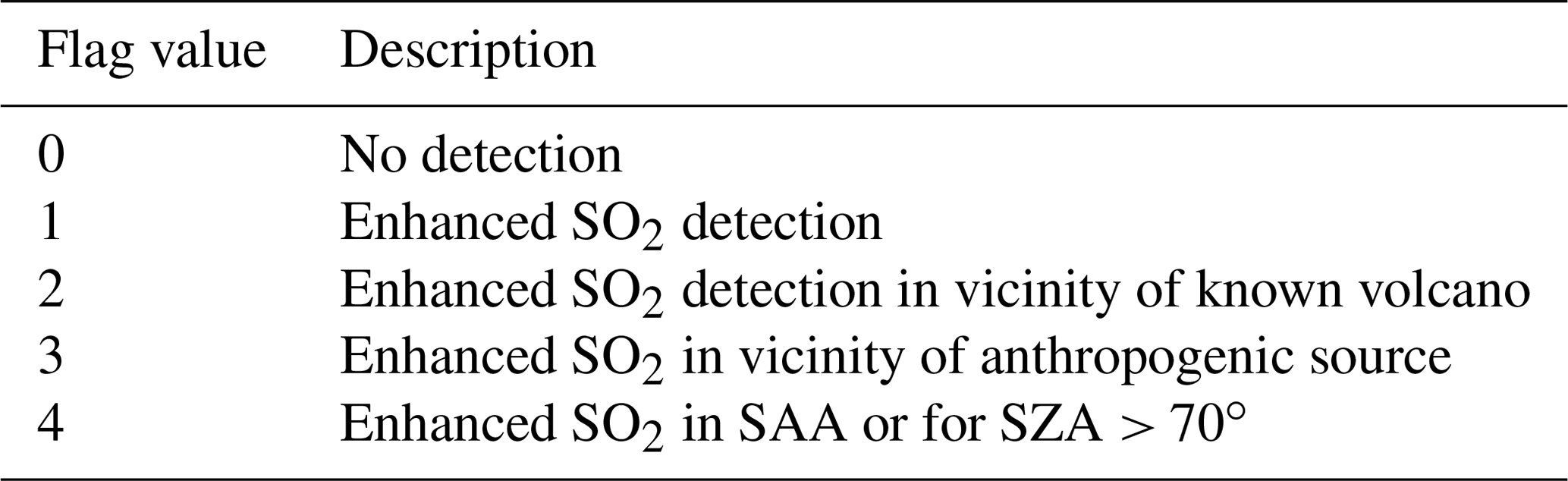
Table 1Volcanic SO2 flags provided for the TROPOMI SO2 products. The same flags are also used for TROPOMI SO2LH data and GOME-2C GPD4.9 SO2 data. SAA is South Atlantic Anomaly, and SZA is solar zenith angle.
2.1 NRT TROPOMI TCSO2 data
TROPOMI, on board the S5P satellite, provides high-resolution spectral measurements in the ultraviolet (UV), visible (Vis), near-infrared and shortwave-infrared parts of the spectrum, allowing several atmospheric trace gases to be retrieved, including SO2 from the UV–Vis part of the spectrum. The horizontal resolution of TROPOMI for the UV–Vis is 5.5 km × 3.5 km (7 km × 3.5 km before 6 August 2019) with daily global coverage. The theoretical baseline for the operational TROPOMI SO2 retrieval is described in Theys et al. (2017), and further information can be found in Algorithm Theoretical Basis Document (ATBD), product user manual (PUM) and readme files available from the TROPOMI website (https://sentinels.copernicus.eu/web/sentinel/user-guides/sentinel-5p-tropomi/document-library, last access: 28 January 2022). The atmospheric SO2 vertical column density is retrieved in three fitting windows (312–326, 325–335 and 360–390 nm) using a Differential Optical Absorption Spectroscopy (DOAS) method (Platt and Stutz, 2008; Platt, 2017), in which the slant SO2 column is retrieved and converted into vertical columns by using air mass factors. The log ratio of the observed UV–Vis spectrum of radiation backscattered from the atmosphere and an observed reference spectrum are used to derive a slant column density, which represents the SO2 concentration integrated along the mean light path through the atmosphere. This is performed by fitting SO2 absorption cross sections to the measured reflectance in a given spectral interval. In a second step, slant columns are corrected for possible biases. Finally, the slant columns are converted into vertical columns by means of air mass factors obtained from radiative transfer calculations, accounting for the viewing geometry, clouds, surface properties and prior SO2 vertical profile shapes. A volcano activity detection algorithm going back to Brenot et al. (2014) is used to identify elevated SO2 values from volcanic eruptions (see Table 1). CAMS only assimilates SO2 pixels that have flag values of 1 (enhanced SO2 detection) or 2 (enhanced SO2 detection in vicinity of known volcano). Furthermore, only TROPOMI SO2 pixels with values greater than 5 DU (Dobson units) are assimilated in the operational CAMS system to avoid assimilating SO2 from outgassing volcanoes that are covered by SO2 emissions in the CAMS model. The TROPOMI SO2 data are “super-obbed”, i.e. in a pre-processing step area means are created by averaging all data (observation values as well as errors) in a model grid box to the model resolution (TL511, about 40 km). These super-observations are then used in the CAMS system without further thinning.
The DOAS vertical column SO2 retrieval requires an assumption for a prior SO2 profile to convert the slant columns into vertical columns. Since this profile shape is generally not known at the time of the observation, and it is also not known whether the observed SO2 is of volcanic origin or from pollution (or both), the TROPOMI algorithm calculates four vertical columns for different hypothetical SO2 profiles. One vertical column is provided for anthropogenic SO2 with the prior SO2 profile taken from the TM5 chemical transport model (CTM), and three columns are provided for volcanic scenarios assuming the SO2 is either located in the boundary layer, in the mid-troposphere (around 7 km) or in the stratosphere (around 15 km), respectively. These volcanic prior profiles are box profiles of 1 km thickness, located at the corresponding altitudes. The NRT CAMS system uses the mid-troposphere product. TROPOMI SO2 data are provided with averaging kernels based on the prior hypothetical SO2 profiles (i.e. the 1 km box profiles centred around the assumed SO2 altitude for the volcanic columns). However, as these do not provide information about the real altitude of a specific volcanic plume they are not used in the CAMS system. More information about the NRT TROPOMI SO2 retrieval can be found in the TROPOMI ATBD. For the TROPOMI data (and also the other SO2 products used in this paper) observation errors as given by the data providers are used within the CAMS data assimilation system.
2.2 FP_ILM NRT TROPOMI layer height data
Hedelt et al. (2019) have developed an algorithm called “Full-Physics Inverse Learning Machine” (FP_ILM) for the retrieval of the SO2 LH based on Sentinel-5 precursor/TROPOMI data using a coupled principal component analysis and neural network approach including regression. This algorithm is an improvement of the original FP_ILM algorithm developed by Efremenko et al. (2017) for the retrieval of the SO2 LH based on GOME-2 data using a principal component regression technique. Recently, this algorithm has also been adapted to retrieve SO2 LH data from the Ozone Monitoring Instrument (OMI) on the Aura satellite (Fedkin et al., 2021). Furthermore, the FP_ILM algorithm has been used for the retrieval of ozone profile shapes (Xu et al., 2017) and the retrieval of surface properties accounting for bidirectional reflectance distribution function effects (Loyola et al., 2020). In general, the FP_ILM algorithm creates a mapping between the spectral radiance and atmospheric parameter using machine learning methods. The time-consuming training phase of the algorithm using radiative transfer model calculations is performed offline, and only the inversion operator has to be applied to satellite measurements, which makes the algorithm extremely fast, and it can thus be used in NRT processing environments. SO2 LH is retrieved in NRT from TROPOMI UV earthshine spectra in the wavelength range 311–335 nm with an accuracy of better than 2 km for SO2 columns greater than 20 DU. For low SO2 columns, high-altitude layer heights cannot be retrieved and the retrieval is biased towards low layer heights (Hedelt et al., 2019). Therefore, the use of the data in the CAMS system is restricted to values > 20 DU. More details about the retrieval algorithm can be found in Hedelt et al. (2019) and Koukouli et al. (2021). Koukouli et al. (2021) compared the S5P LH data with IASI observations for the 2019 Raikoke, 2020 Nishinoshima and 2021 La Soufrière-St Vincent eruptive periods and found good agreement with a mean difference of ∼ 0.5 ± 3 km, while for the 2020 Taal eruption a larger difference of between 3 and 4 ± 3 km was found. In this paper we use version 3.1 of the FP_ILM SO2 LH products.
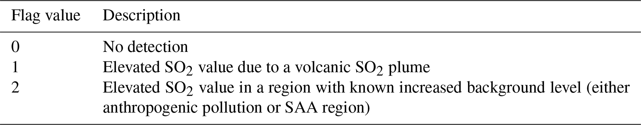
Table 2Volcanic SO2 flags provided for the GDP4.8 GOME-2A and GOME-2B SO2 products.
2.3 NRT GOME-2 TCSO2 data
GOME-2 (Munro et al., 2016) on board the MetOp-A, MetOp-B and MetOp-C satellites, measures in the UV–Vis part of the spectrum (240–790 nm). MetOp-B and MetOp-C have a swath of 1920 km at 40 km × 80 km ground pixel resolution, while MetOp-A has a narrower swath of 960 km at 40 km × 40 km. Global coverage with GOME-2 is achieved within 1.5 d. The GOME-2 measurements allow for the retrieval of ozone and a range of atmospheric trace gases, including SO2 which is retrieved with the GOME Data Processor (GDP) developed by DLR and operationally provided by the EUMETSAT's ACSAF that uses a DOAS method. GDP4.8 is used for GOME-2A and GOME-2B (with a fitting window from 315–326 nm), and GDP4.9 is used for GOME-2C (with a fitting window of 312–326 nm to include the strong SO2 line at 313 nm). Input parameters for the DOAS fit include the absorption cross section of SO2 and the absorption cross sections of interfering gases, ozone and NO2, and a correction is made in the DOAS fit to account for the ring effect (rotational Raman scattering). An empirical interference correction is applied to the SO2 slant column values to reduce the interference from ozone absorption (Rix et al., 2012). To reduce the interference from ozone absorption, the retrieval includes the fitting of two pseudo-ozone cross sections following the approach of Puķīte et al. (2010). As in the case for the TROPOMI dataset, a volcano activity detection algorithm is used to identify elevated SO2 values from volcanic eruptions. Such flags were implemented in GDP4.8 (see Table 2) and further improved in GDP4.9 to use the same flagging as for TROPOMI (see Table 1). CAMS only assimilates the GOME-2 SO2 data that are flagged as volcanic (value of 1 for GDP4.8; value of 1 or 2 for GDP4.9) and assimilates GOME-2B and GOME-2C in the NRT system operational in 2021. The GOME-2 data are used at the satellite resolution, which is similar to the resolution of the CAMS model used in this paper. In this paper only SO2 data from GOME-2B are used.
2.4 IASI SO2 plume altitude data
The Infrared Atmospheric Sounding Instrument (IASI) is flying on board EUMETSAT's MetOp-A (since 2006), MetOp-B (since 2012) and MetOp-C (since 2017) satellite platforms (Clerbaux et al., 2015). The instruments measure the upwelling radiances in the thermal infrared spectral range extending from 645 to 2760 cm−1 with high radiometric quality and 0.5 cm−1 spectral resolution. A total of 120 views are collected over a swath of ∼ 2200 km using a stare-and-stay mode of 30 arrays of four individual elliptical pixels, each of which is 12 km diameter at nadir, increasing at the larger viewing angles. IASI provides global monitoring of total ozone, carbon monoxide, methane, ammonia, nitric acid and SO2, among other atmospheric constituents. The IASI/MetOp SO2 columnar data are operationally provided by the EUMETSAT's ACSAF. In Clarisse et al. (2012) a novel algorithm for the sounding of volcanic SO2 plumes above ∼5 km altitude was presented and applied to IASI observations. The algorithm is able to view a wide variety of total column ranges (from 0.5 to 5000 DU), exhibits a low theoretical uncertainty (3 %–5 %) and near real-time applicability, as demonstrated for the recent eruptions of Sarychev in Russia, Kasatochi in Alaska, Grimsvötn in Iceland, Puyehue-Cordon Caulle in Chile, and Nabro in Eritrea (Tournigand et al., 2020.) A validation of this algorithm on the Nabro eruption observations using forward trajectories and CALIOP/CALIPSO space-borne lidar coincident measurements is presented in Clarisse et al. (2014), where the expansion of the algorithm to also provide SO2 plume altitudes is further described. The IASI/MetOp SO2 ACSAF product includes five SO2 column data at assumed layer heights of 7, 10, 13, 16 and 25 km, as well as a retrieved best estimate for the SO2 plume altitude and associated SO2 column. Note that the SO2 plume altitudes provided by this algorithm are quantized every 0.5 km. This dataset is publicly available from https://iasi.aeris-data.fr/SO2_iasi_a_arch/ (last access: 28 January 2022).
For the requirements of the validation against the CAMS experiments, all available IASI SO2 plume altitude data for the Raikoke volcano 2019 eruption were gridded onto a 1∘ × 1∘ grid at 3 h intervals per day. The equivalent CAMS SO2 plume altitude, i.e. the altitude where the maximum SO2 load occurs in the CAMS SO2 profiles, was chosen for the collocations. In the case where two CAMS altitudes provided the same SO2 load, the mean was assigned as the CAMS SO2 plume altitude.
3.1 CAMS volcanic SO2 plume forecasting system
The chemical mechanism of ECMWF's Integrated Forecast System (IFS) is a modified and extended version of the Carbon Bond 2005 chemistry scheme (CB05, Yarwood et al., 2005) chemical mechanism for the troposphere, as also implemented in the chemical transport model (CTM) TM5 (Huijnen et al., 2010). CB05 is a tropospheric chemistry scheme with 57 species and 131 reactions. The chemistry module of the IFS is documented in more detail in Flemming et al. (2015) and Flemming et al. (2017), and more recent updates are detailed in Inness et al. (2019). The CB05 chemistry scheme is coupled to the AER aerosol bulk scheme (Rémy et al., 2019) for the simulation of sulfate, nitrate and ammonium aerosols. More up-to-date information is available from http://atmosphere.copernicus.eu (last access: 28 January 2022).
In the original version of the volcanic SO2 plume forecasting system described by Flemming and Inness (2013), there was a dedicated “volcanic SO2 tracer”, with oxidation based on a simple fixed timescale approach. By contrast, in the progression of the volcanic SO2 system described here, the volcanic SO2 emissions and data assimilation of SO2 are applied to the SO2 tracer within the CB05 chemistry scheme (Flemming et al., 2015), with oxidation to sulfate aerosol occurring based on the kinetics specified in the chemistry scheme. There are two pathways for this (i) in the gas phase via the hydroxyl radical (OH) and (ii) within cloud droplets (aqueous phase), with only pathway (i) occurring in the stratosphere (in the model). In the troposphere, the model also includes the SO2 loss processes of wet deposition and surface dry deposition. Although heterogenous SO2 oxidation on ash particles and the self-lofting effect from the ash heating effect have both been shown to be important for the SO2 dispersion from Raikoke (Muser et al., 2020) and also from the 2015 Kelud eruption (Zhu et al., 2020), ash particles are not included in these IFS simulations.
As described in Flemming et al. (2015) the IFS uses a semi-Lagrangian advection scheme. Since the semi-Lagrangian advection does not formally conserve mass, a global mass fixer is applied to the chemical tracers, including to the SO2 tracer, and a proportional mass fixer as described in Diamantakis and Flemming (2014) was used for the runs presented in this paper. More details about the CB05 chemistry scheme can be found in Flemming et al. (2015, 2017), Réemy et al. (2019) and Huijnen et al. (2019).
The model version used in this paper is based on the IFS model cycle 47R1 (CY47R1, http://www.ecmwf.int/en/forecasts/documentation-and-support/changes-ecmwf-model, last access: 28 January 2022), which was the operational CAMS cycle from 6 October 2020 to 18 May 2021. In CY47R1, the CAMS system uses the CAMS-GLOBANTv4.2 anthropogenic emissions (Granier et al., 2019), which include anthropogenic SO2, as well as a climatology of SO2 outgassing volcanic emissions based on satellite data (Carn et al., 2016). Further updates relative to the previous version (CY46R1) are as follows:
-
a change to Global Fire Assimilation System (GFAS) v1.4 biomass-burning emissions;
-
the exclusion of agricultural waste burning from CAMS_GLOB_ANT to avoid double-counting with GFAS;
-
the use of an improved diurnal cycle and vertical profile for anthropogenic emissions;
-
the introduction of the Hybrid Linear Ozone (HLO) scheme, a Cariolle-type linear parameterization of stratospheric ozone chemistry using the multi-year mean of the CAMS reanalysis as mean state;
-
an update to the dust source function, which reduces the overestimation of dust in the Sahara, Middle East and other regions and restores missing dust over Australia;
-
the use of a new sea salt emission scheme based on Albert et al. (2016) that provides better agreement with measured sea salt size distribution;
-
the use of revised coefficients in the UV processor based on the ATLAS3 spectrum.
3.2 CAMS data assimilation system
The IFS uses an incremental four-dimensional variational (4D-Var) data assimilation system (Courtier et al., 1994). In the CAMS 4D-Var a cost function that measures the differences between the model fields and the observations is minimized to obtain the best possible forecast through the length of the assimilation window by adjusting the initial conditions. SO2 is one of the atmospheric composition fields that is included in the control vector and minimized together with the meteorological control variables in the CAMS system (Inness et al., 2015; Flemming and Inness, 2013). The current operational CAMS configuration uses a weak constraint formulation of 4D-Var, which includes a model error term for the meteorological variables (Laloyaux et al., 2020) that mainly corrects the stratospheric temperature bias and also slightly improves the stratospheric winds. In the CAMS 4D-Var system, the control variables are the initial conditions at the beginning of the assimilation window, with the aim of providing the best initial conditions for the subsequent forecast. The background error covariance matrix in the ECMWF data assimilation system is given in a wavelet formulation (Fisher, 2004, 2006). This allows for both spatial and spectral variations of the horizontal and vertical background error covariances. The CAMS background errors are constant in time. The horizontal resolution of the NRT CAMS 2021 operational system, as well as that of the data assimilation experiments presented in this paper, is approximately 40 km, corresponding to a triangular truncation of TL511 or a reduced Gaussian grid with a resolution of N256 (more information can be found at https://confluence.ecmwf.int/display/FCST/Gaussian+grids, last access: 28 January 2022). The operational CAMS system uses two minimizations (the so-called inner loops) at reduced horizontal resolution, currently at TL95 and TL159, corresponding to horizontal resolutions of about 210 km and 125 km. This means that wavenumbers up to 95 and 159, respectively, can be represented in the wavelet formulation for the background errors. For the experiments presented in this paper, slightly higher horizontal resolutions of TL159/TL255 were used for the inner loops (corresponding to about 125 and 80 km, respectively). The CAMS model and data assimilation system has 137 model levels in the vertical between the surface and 0.01 hPa and uses a 12 h 4D-Var configuration with assimilation windows from 03:00 to 15:00 UTC and from 15:00–03:00 UTC.
3.2.1 CAMS NRT TCSO2 assimilation configuration (baseline configuration)
The SO2 data assimilated in the CAMS NRT configuration are total column values. To calculate the model equivalent of the observations the CAMS SO2 field is interpolated to the time and location of the measurements, and the CAMS SO2 columns are calculated as a simple vertical integral between the surface and the top of the atmosphere. While the background error statistics for most of the atmospheric composition fields (Inness et al., 2015) were either calculated with the National Meteorological Center (NMC) method (Parrish and Derber, 1992) or from an ensemble of forecast differences (following a method described by Fisher and Andersson, 2001), the background errors for SO2 are prescribed by an analytical vertical standard deviation profile and horizontal correlations. SO2 observations are currently only assimilated in the CAMS system in the event of volcanic eruptions. An NMC or ensemble approach would not give useful SO2 background error statistics in these cases as the forecast model does not have information about individual volcanic eruptions, even though it does include emissions from outgassing volcanoes. SO2 background error standard deviations calculated with the NMC or ensemble methods peak near the surface where anthropogenic SO2 concentrations are largest and will hence lead to the largest analysis increments near the surface. Therefore, for the assimilation of volcanic SO2 data, background error statistics for SO2 were constructed by prescribing a background error standard deviation profile that is a delta function and peaks in the mid-troposphere around model level 98 (about 550 hPa) in the 137 level model version, corresponding to an SO2 plume height of about 5 km (see blue profile in Fig. 1).
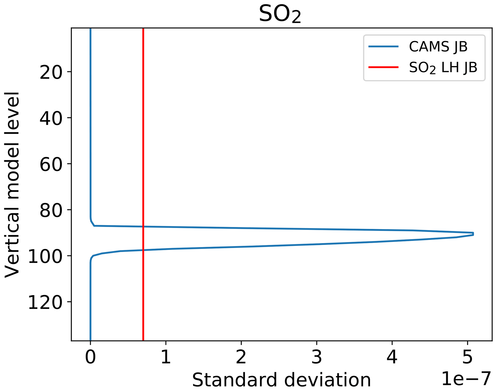
Figure 1Vertical profile of SO2 background error standard deviation (in kg kg−1) used in the operational CAMS configuration (blue) and for the main LH experiment (red, LHexp). The y axis shows model levels. Level 1 is the top of the atmosphere, and level 137 is the surface.
The SO2 wavelet file in the NRT CAMS configuration (also called baseline configuration in this paper) is formed of diagonal vertical wavenumber correlation matrices, with the value on the diagonal controlled by a horizontal Gaussian correlation function with a standard deviation of 250 km and a globally constant vertical standard deviation profile. The values of the elements on the diagonal of the vertical correlation matrix are the same at every level but vary for each wavenumber. If TCSO2 data are assimilated, the largest correction to the model's background will be applied where the background errors are largest, i.e. in the mid-troposphere around 550 hPa. The CAMS SO2 analysis is univariate, meaning that there are no cross correlations between SO2 background errors and the other atmospheric composition control variables.
3.2.2 Data assimilation configuration for TCSO2 LH data
If information about the altitude of the volcanic SO2 layer is known in NRT, a different approach can be followed. In this case, we use a background error standard deviation profile that is constant in height (e.g. the red line in Fig. 1) and calculate the SO2 column not between the surface and the top of the atmosphere but instead between the pressure values that correspond to the bottom and the top of the retrieved volcanic SO2 layer. The depth of this layer is currently set in the FP_ILM product as 2 km, which corresponds to the uncertainty of the retrieved layer height. This approach mimics the procedure of using TROPOMI SO2 averaging kernels, which are box profiles, but for the retrieved layer and not an assumed hypothetical volcanic SO2 profile (see TROPOMI SO2 ATBD, http://www.tropomi.eu/documents/, last access: 28 January 2022). One limitation of this method is that the SO2 LH product gives the plume altitude with an accuracy of 2 km but does not give a value for the lower vertical boundary of the SO2 plume, and for a thick part of the SO2 plume loading could be missed in the calculation of the model equivalent. However, as the model's background SO2 concentrations in the free troposphere are low, this should not be a big issue in the column calculation. In addition, some vertical variation of the SO2 loading will result from assimilating observations with varying plume altitudes for larger volcanic plumes that are not uniform in height everywhere, and Fig. 3 below shows that this is indeed the case for the Raikoke eruption. Results from sensitivity studies regarding the choice of the constant background error standard deviation value are given below in Sect. 4.2.
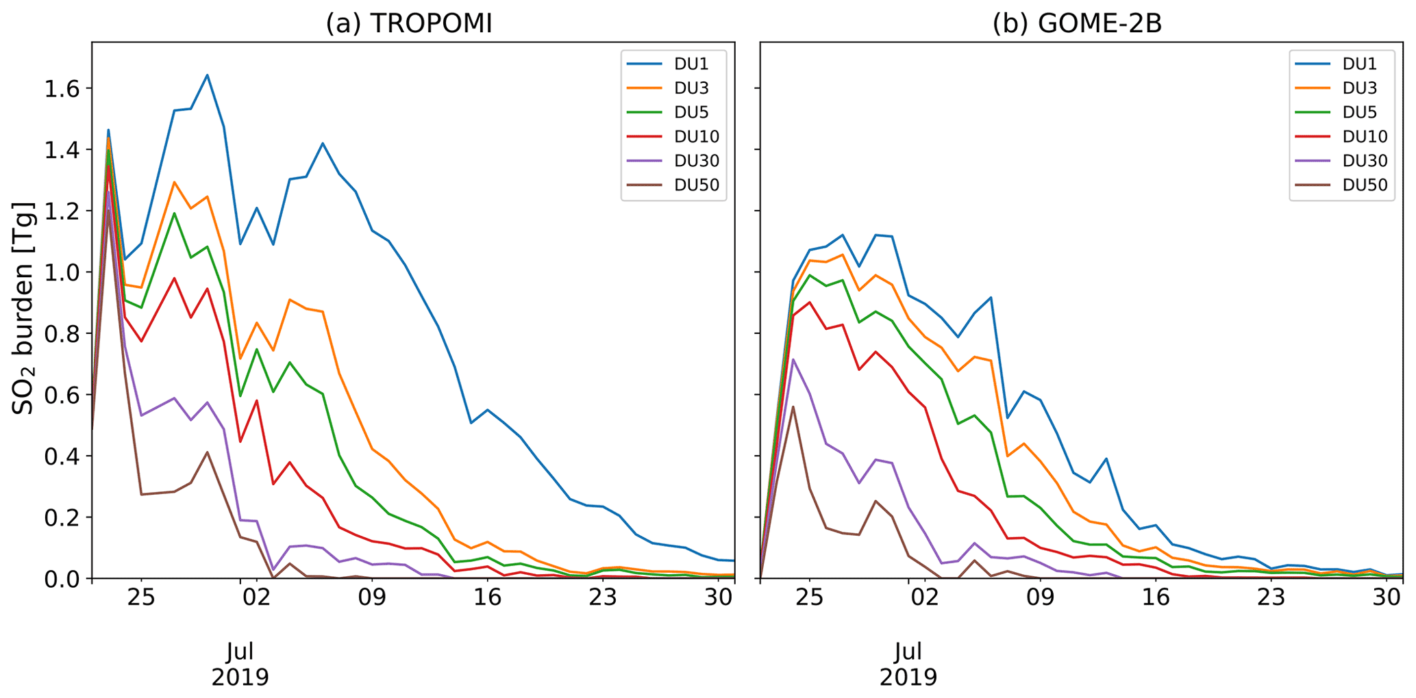
Figure 2SO2 burden (in Tg) from TROPOMI (a) and GOME-2B (b) from 22 June to 31 July 2019. The values are calculated by gridding the data on a 1∘ × 1∘ grid and selecting the grid cells with TCSO2 values greater than thresholds of 1, 3, 5, 10, 30, and 50 DU in the area 30–90∘ N.
4.1 Raikoke eruption June 2019
The Raikoke volcano, located on the Kuril Islands south of the Kamchatka Peninsula, erupted around 18:00 UTC on 21 June 2019 and emitted SO2 and ash in a series of explosive events until about 06:00 UTC on 22 July. The SO2 and ash plume rose to around 8–18 km (Muser et al., 2020; Grebennikov et al., 2020) meaning a considerable amount of the SO2 reached the stratosphere. The volcanic cloud was transported around much of the Northern Hemisphere, was observed by TROPOMI and GOME-2 for about a month and was also observed with ground-based measurements (Vaughan et al., 2021; Grebennikov et al., 2020) and other satellites (Muser et al., 2020). Figure 2 shows the TCSO2 burden from the Raikoke eruption as calculated from NRT TROPOMI and GOME-2B data. All the TCSO2 satellite data available during a 12 h assimilation window were gridded onto a 1∘ × 1∘ degree grid and the area of all grid cells with SO2 values greater than the listed threshold values was calculated. For a threshold of 1 DU, the SO2 burdens from TROPOMI and GOME-2B were around 1.5 and 1.1 Tg, respectively. These values agree with findings by de Leeuw et al. (2021) and make the eruption the largest since the eruption of the Nabro volcano in 2011 (de Leeuw et al., 2021; Goitom et al., 2015; Clarisse et al., 2014). The “dip” in the TROPOMI SO2 burden after the initial peak is an artefact that results from missing observations in the TROPOMI NRT data on 25 June 2019 in the area of highest SO2 values (also visible in Fig. 9c2 below).
Figure 3 shows a time series of the SO2 LH information from the TROPOMI LH product for the Raikoke plume. It shows that volcanic SO2 can be detected and the SO2 LH information retrieved for about 3 weeks after the eruption. The bulk of the SO2 was located above 300 hPa, (about 9 km), with a considerable amount above 200 hPa (about 12 km). This is considerably higher than the 550 hPa that is assumed as the plume location in the CAMS operational (baseline) configuration. Large TCSO2 values (> 100 DU) were observed in the first days after the eruption.
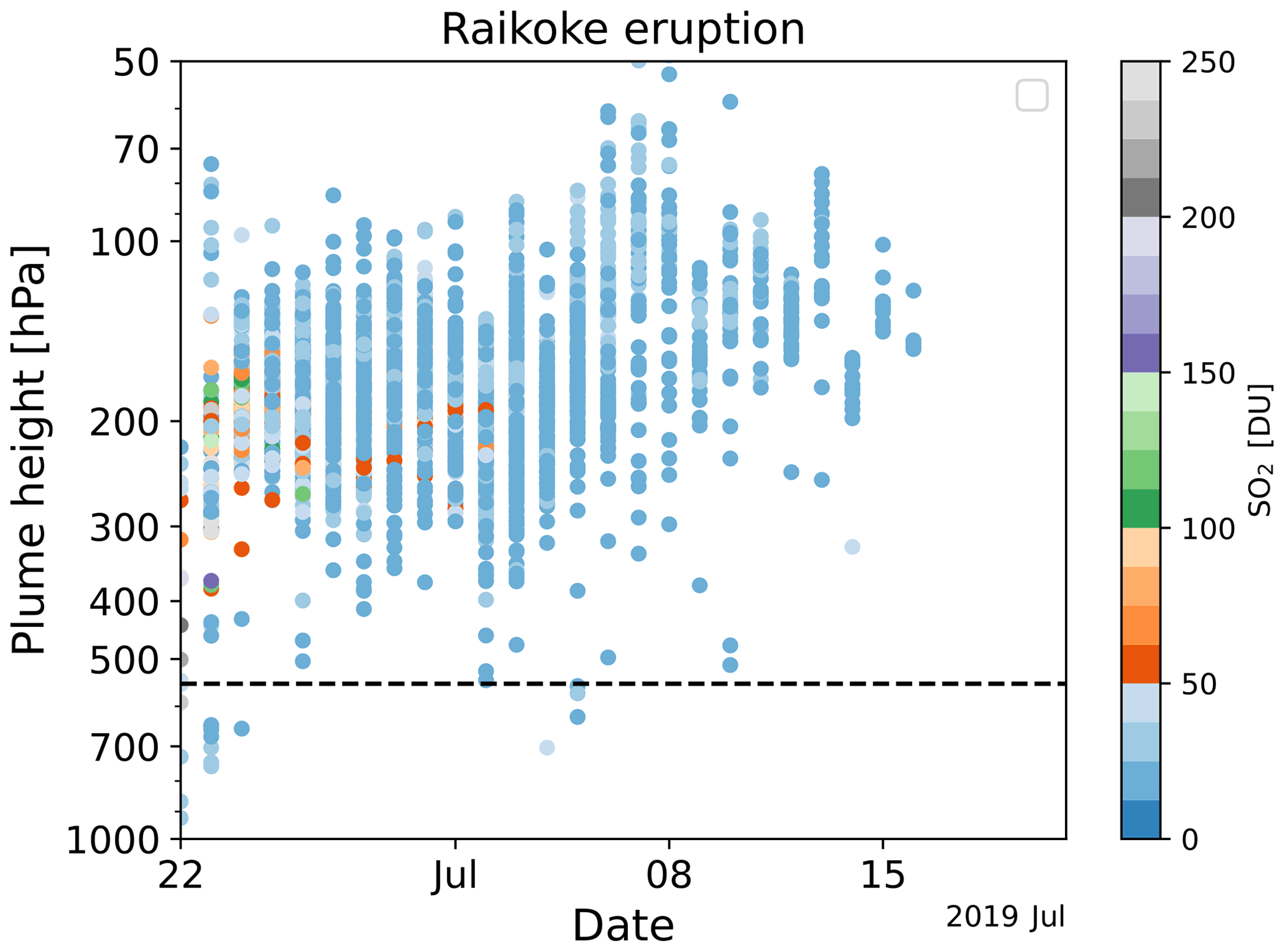
Figure 3Time series of the height of the Raikoke volcanic plume (averaged over 30–90∘ N) in hPa from TROPOMI SO2 LH data from 22 June to 21 July 2019. The colours show the corresponding TCSO2 values in DU. The dashed horizontal line at 550 hPa shows the altitude where the CAMS baseline configuration places the maximum SO2 increment.
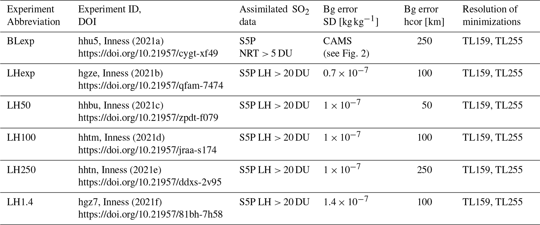
Table 3List of SO2 assimilation experiments used in this paper. The main experiments discussed in Sect. 4 are the baseline experiment (BLexp) and the layer height experiment (LHexp). The additional experiments are used in the sensitivity studies in Sect. 4.2. Bg error denotes background error, SD denotes standard deviation and hcor denotes horizontal correlation length scale.
4.2 Sensitivity studies for assimilation of TCSO2 data
Several data assimilation experiments were run for the period 22 June to 21 July 2019 to test the assimilation of the SO2 LH data and to compare the results with the CAMS baseline configuration listed in Table 3. The baseline experiment (BLexp), which assimilated NRT TROPOMI TCSO2 data with the operational CAMS configuration, and the layer height experiment (LHexp), which uses the FP_ILM S5P LH data with a horizontal background error correlation length of 100 km and background error standard deviation values of 0.7 × 10⁻⁷ kg kg−1, are the main experiments used in this paper (Sect. 4.3 below) to assess if the assimilation of the SO2 LH data using a more realistic height rather than the default 5 km improves the CAMS SO2 analyses and forecasts. The other LH experiments assess the impact of using different horizontal SO2 background error correlation length scales and various SO2 background error standard deviation values. In all of these experiments GOME-2 SO2 data were not assimilated, and GOME-2B is used as a fully independent dataset for the validation.
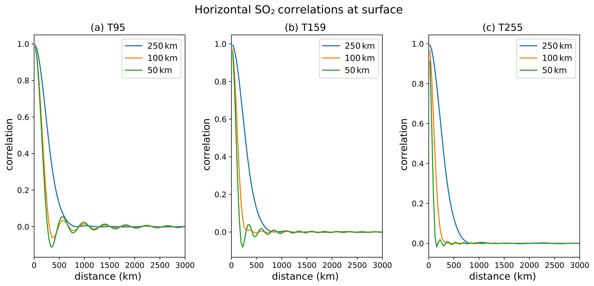
Figure 4SO2 background error horizontal surface correlations at different truncations, i.e. (a) TL95, (b) TL159 and (c) TL255, where the horizontal length scales are specified as Gaussian correlation function with length scales of 250 km (blue), 100 km (orange) and 50 km (green), respectively.
The low resolution of the minimization (TL95 and TL159 in the CAMS system operational in 2021) is a factor that limits the ability of the SO2 analysis to reproduce small-scale SO2 features seen in the observations because it gives a lower limit for the length scale of the horizontal background error correlations that can be used, i.e. for the operational CAMS configuration only wavenumbers up to 95 and 159 (for TL95 and TL159, respectively) can be represented. The smallest wavelength (λmin) that can be represented by two grid points on a linear grid is
where R is the radius of the Earth and nmax the maximum wavenumber of the truncation (95 or 159 for the inner loops in the operational CAMS configuration), i.e. twice the size of a grid box. This means that the minimum wavelengths that can be represented with two grid points for TL95, TL159 and TL255 are about 420, 250 and 160 km, respectively, and smaller-scale horizontal structures cannot be represented in the background error wavelet formulation. Figure 4 illustrates this and shows horizontal SO2 correlations at the surface for horizontal background error length scales of 50, 100 and 250 km for truncations of TL95, TL159 and TL255. The “wriggles” seen in the TL95 (and to a lesser extent in the TL159) plots show that the shorter background error correlations length scales cannot be properly resolved at these truncations. Even at TL255 some minor oscillations are still visible for horizontal correlation length scales of 50 km. Therefore, to properly resolve smaller-scale plumes the resolutions of the inner loops would need to be even higher than TL255. Figure 4 also illustrates how far an increment from a single SO2 observation would be spread out in the horizontal and therefore affect grid points away from the observation.
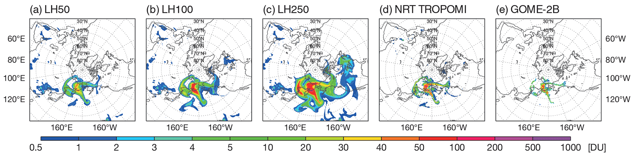
Figure 5TCSO2 analyses on 27 June 2019 at 00:00 UTC obtained by assimilating SO2 LH data using a background standard deviation profile of 10−7 kg kg−1 and background errors with horizontal correlations of (a) 50 km, (b) 100 km and (c) 250 km. Also shown are (d) NRT TROPOMI and (e) GOME-2B TCSO2 values.
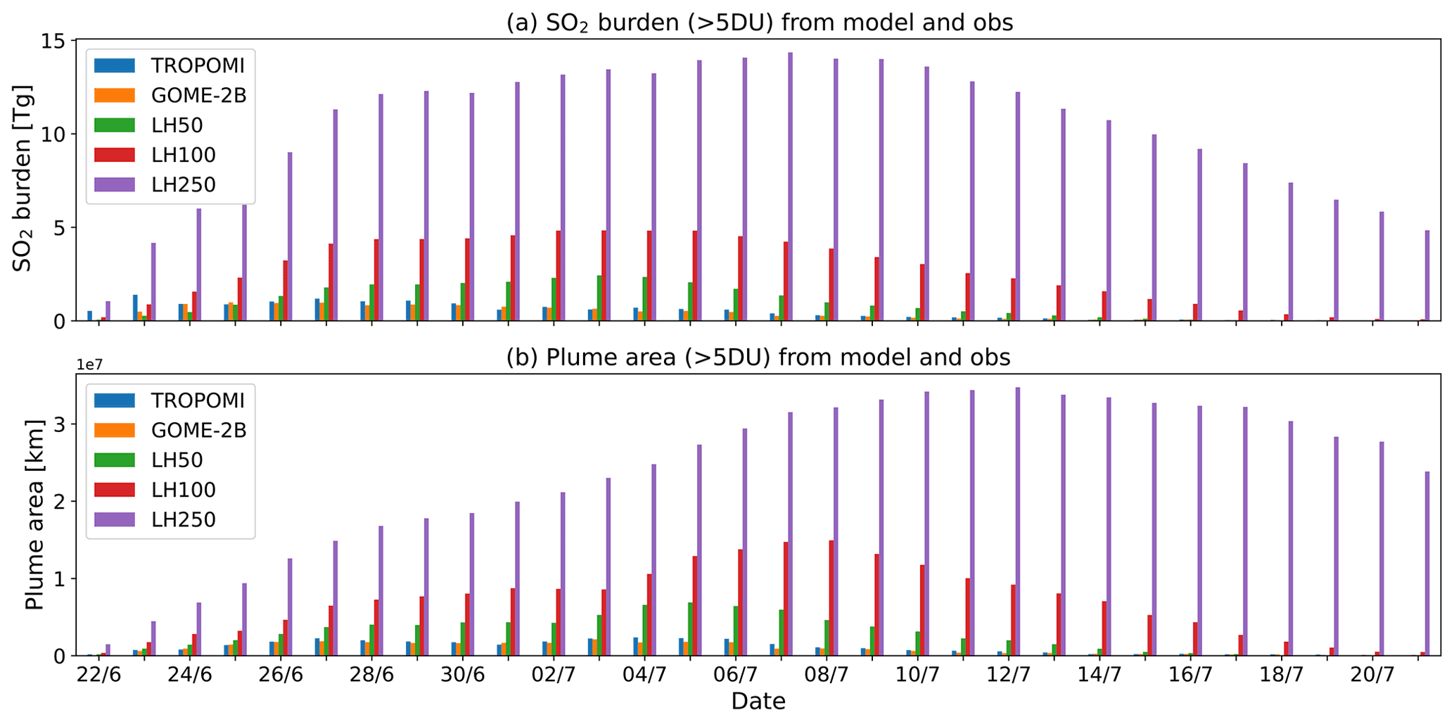
Figure 6(a) SO2 burden (in Tg) and (b) plume area (in 1 × 10⁷ km2) from TROPOMI, GOME-2B and three SO2 LH experiments at 00:00 UTC with horizontal background error length scales of 50 km (LH50), 100 km (LH100) and 250 km (LH250) for the Raikoke eruption (22 June to 21 July 2019). The values are calculated by gridding the data on a 1∘ × 1∘ grid and selecting the grid cells with TCSO2 values greater than 5 DU in the area 30–90∘ N.
The operational NRT CAMS configuration uses minimizations at TL95 and TL159 and a length scale of 250 km for the horizontal SO2 background error correlations. For the data assimilation experiments shown in this paper we use inner loops of TL159 and TL255 to allow us to use a Gaussian correlation function with a length scale of 100 km and therefore resolve slightly smaller-scale features than in the operational NRT CAMS system. The computational cost of one analysis cycle increases by about 20 %–30 % when the spectral resolution of the minimization is increased in this way, with the largest increase coming from the second minimization, which is about 50 % computationally more expensive than at lower resolution. Figure 5 shows the CAMS TCSO2 analysis fields on 27 June 2019 resulting from the assimilation of the TROPOMI SO2 LH data when horizontal background error correlation length scales of 50, 100 and 250 km were used (experiments LH50, LH100, LH250), while using the same background error standard deviation profile of 1 × 10⁻⁷ kg kg−1 in all cases. Also shown are the NRT TROPOMI and GOME-2B TCSO2 data for that day. The figure illustrates the large impact of the horizontal background error correlation length scale on the SO2 analysis, as the SO2 plume is considerably more spread out in the CAMS analysis when longer horizontal correlations are used, and shows that better agreement with the features seen in the observations is found for shorter horizontal correlations. Figure 6 shows time series of SO2 burden and plume area for a threshold of 5 DU from TROPOMI, GOME-2B and the three SO2 LH experiments to further assess the impact on the SO2 analysis of changing the horizontal correlation length scale. We see that the SO2 burden and plume area calculated from the observations are overestimated by all three CAMS TCSO2 analyses. This overestimation is a well-known feature usually seen in the operational NRT CAMS volcanic SO2 assimilation. Figure 6 illustrates that a major factor causing this overestimation is the choice of the horizontal background error correlation length scale and that by choosing a length scale of 250 km the SO2 burden and plume area are about 6 times larger than for a length scale of 50 km. This implies that a limiting factor for correctly reproducing the SO2 burden and plume area in the CAMS analysis is the resolution of the inner loops, as it limits the horizontal correlation length scale that can be chosen for the background errors. A coarser inner loop resolution requires a longer horizontal length scale because shorter wavelengths cannot be resolved properly. If the aim is to reproduce finer-scale volcanic plumes with the CAMS data assimilation system, the horizontal resolution of the inner loops will have to be increased. For the main LH experiment used in this paper we decided to use a horizontal correlation length scale of 100 km, which can be represented properly if the resolutions of the inner loops are TL159 and TL255.
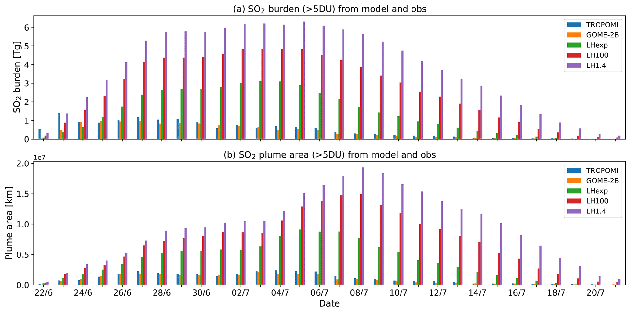
Figure 7(a) SO2 burden (in Tg) and (b) plume area (in 1 × 10⁷ km2) from TROPOMI, GOME-2B and three SO2 LH experiments at 00:00 UTC with background error standard deviation values of 0.7 × 10⁷ (LHexp), 1 × 10⁻⁷ (LH100) and 1.4 × 10⁻⁷ kg kg−1 (LH1.4) for the Raikoke eruption (22 June to 21 July 2019). The values are calculated by gridding the data on a 1∘ × 1∘ grid and selecting the grid cells with TCSO2 values greater than 5 DU in the area 30–90∘ N.
Another factor that influences the results of the SO2 analysis is the value of the background error standard deviation profile. This is illustrated in Fig. 7, which shows time series of SO2 burden and plume area from TROPOMI, GOME-2B and three SO2 LH experiments with varying background error standard deviation values (0.7 × 10⁻⁷, 1.0 × 10⁻⁷ and 1.4 × 10⁻⁷ kg kg−1). All experiments used a horizontal background error correlation length scale of 100 km. The larger the background error standard deviation, the larger the correction that is made by the SO2 analysis and the larger the SO2 burden and plume area become. However, the impact of changing the background error standard deviation is not as big as changing the horizontal background error correlation length scale, and increasing the standard deviation value from 0.7 × 10⁻⁷ to 1.4 × 10⁻⁷ kg kg−1 doubles the SO2 burden and plume area.
For the remainder of this paper, the LH experiment that uses a value of 0.7 × 10⁻⁷ kg kg−1 for the background error standard deviation and a horizontal background error correlation length scale of 100 km is used (abbreviated as LHexp).
4.3 Results of TCSO2 assimilation tests for the Raikoke 2019 eruption
The SO2 analysis fields and 5 d forecasts for the Raikoke eruption from the SO2 layer height experiment (LHexp) and the baseline experiment with the CAMS configuration (BLexp) are now assessed in more detail. This assessment includes (i) a visual inspection of the SO2 analysis, (ii) the assessment of the vertical location of the analysis SO2 plume by comparison with independent IASI/MetOp plume height observations, and (iii) the assessment of the quality of the 5 d SO2 forecasts that are started from the LHexp and BLexp SO2 analyses.
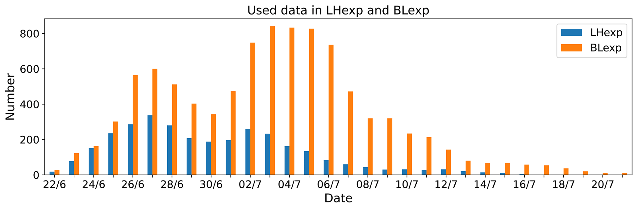
Figure 8Time series of the number of active TROPOMI SO2 observations assimilated in LHexp (blue) and BLexp (orange) gridded on a 1∘ × 1∘ grid (22 June to 21 July 2019).
We evaluate the SO2 analyses and forecasts against GOME-2B and TROPOMI NRT TCSO2 data. GOME-2B TCSO2 data are fully independent because they are not used in our SO2 assimilation experiments, and TROPOMI NRT TCSO2 products are useful to demonstrate how well the analyses manage to reproduce the TROPOMI TCSO2 values. It has to be kept in mind that the version of the SO2 LH product used in this study (v3.1) attains its optimal accuracy of 2 km for SO2 columns greater than 20 DU, and hence in LHexp no TCSO2 observations below 20 DU are assimilated. For the evaluation, the SO2 analyses and forecasts, as well as the satellite data, are gridded onto a 1∘ × 1∘ grid. Figure 8 shows a time series of the number of observations that are actively assimilated in both experiments, i.e. the number of 1∘ × 1∘ grid points with active observations, and illustrates that there are more active data in BLexp where NRT TROPOMI SO2 data with values greater than 5 DU are assimilated (i.e. as done in the operational CAMS system) than in LHexp where only data with LH TCSO2 greater than 20 DU are assimilated.
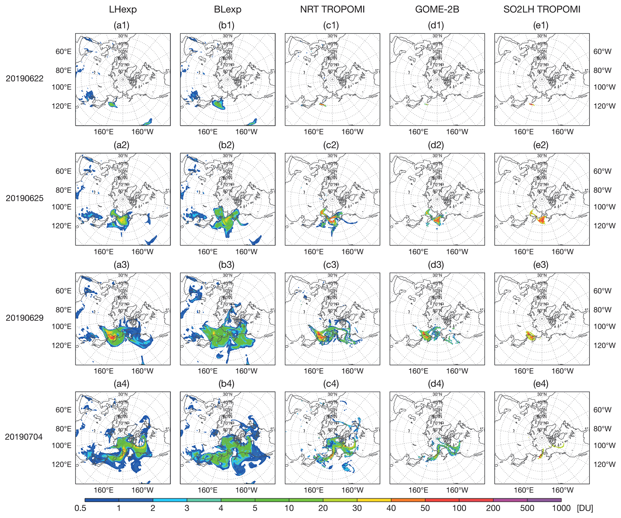
Figure 9TCSO2 analysis fields at 00:00 UTC from LHexp (a), BLexp (b), NRT TROPOMI (c), NRT GOME-2B (d) and TROPOMI SO2LH (e) on 22 June (row 1), 25 June (row 2), 29 June (row 3) and 4 July (row 4) in DU. In column (c–e) all available observations are shown, illustrating that the SO2 LH product only picks up those parts of the plume that are associated with the highest SO2 load.
4.3.1 Evaluation of TCSO2 analyses
Figure 9 shows TCSO2 maps from LHexp and BLexp, as well as maps of TCSO2 from NRT TROPOMI, GOME-2B and FP_ILM TROPOMI SO2LH data, for 4 d: 22, 25, 29 June and 4 July 2019. The maps on 22 June capture the beginning of the eruption and show that the TCSO2 values from the first analysis cycle in both experiments are lower than the observations. It also illustrates that even at this initial time the extent of the SO2 plume is overestimated in both experiments. By 25 and 29 June the SO2 plume already covers a big part of the North Pacific, and by 4 July SO2 from the eruption is detected in half the Northern Hemisphere. LHexp captures the structures of the SO2 plumes seen in the observations better than BLexp, but overall both experiments capture the horizontal extent of the plume reasonably well. Figure 9 also illustrates that GOME-2B and NRT TROPOMI TCSO2 show the same features of the plume; however, the TROPOMI NRT lower detection limit facilitates the retrieval of smaller TCSO2 values around the edges of the plumes. The FP_ILM SO2LH product (v3.1) does not provide reliable information for TCSO2 < 20 DU and therefore only picks up those parts of the plume that are associated with the highest SO2 load. This also explains the lower number of active observations seen in Fig. 8. Parts of the plume are missed by the SO2 LH product, especially during the later stages of the eruption. Nevertheless, when assimilating the FP_ILM SO2 LH data we find good agreement with the NRT TROPOMI data and the GOME-2B data in LHexp (Fig. 9, column 1) when the CAMS analysis reports SO2 values <20 DU.
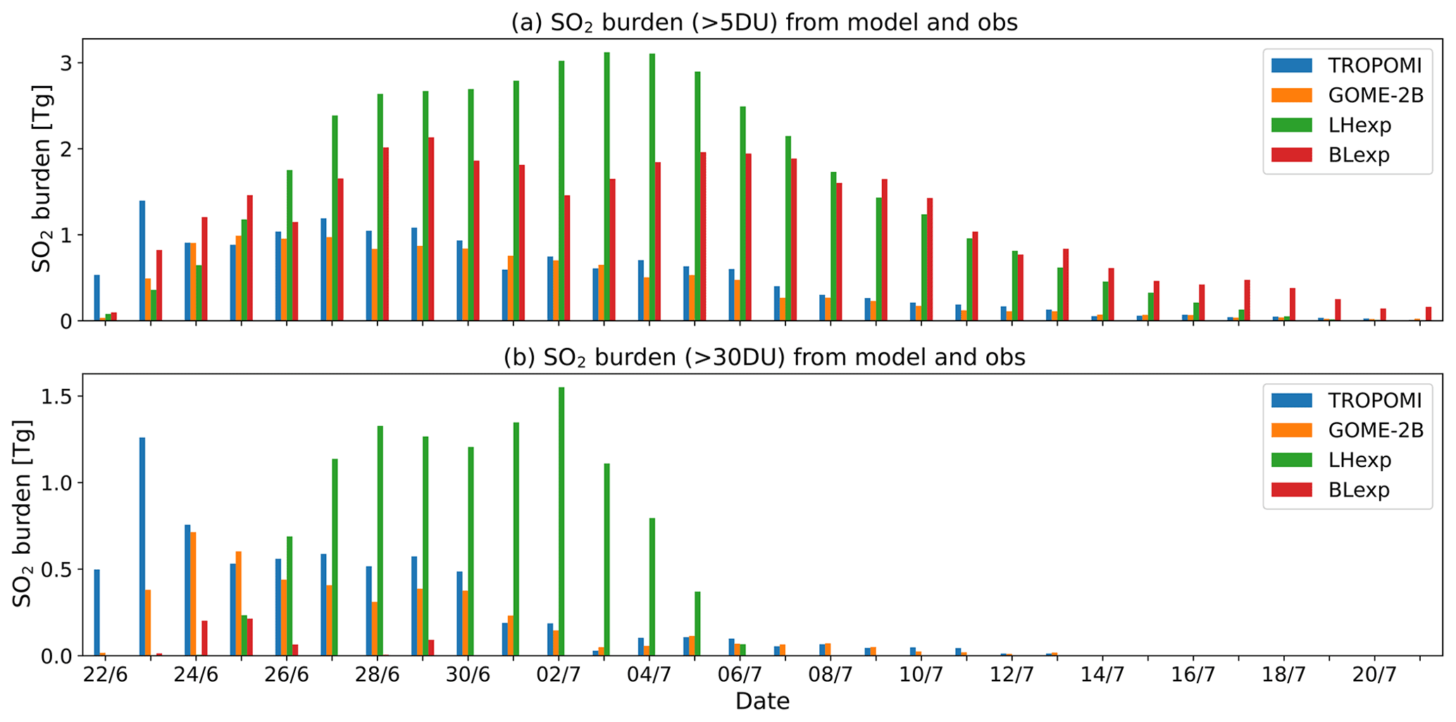
Figure 10SO2 burden (in Tg) from TROPOMI, GOME-2B, LHexp and BLexp TCSO2 analysis at 00:00 UTC for the Raikoke eruption (22 June to 21 July 2019). The values are calculated by gridding the data on a 1∘ × 1∘ grid and selecting the grid cells with TCSO2 values greater than (a) 5 DU and (b) 30 DU in the area 30–90∘ N.
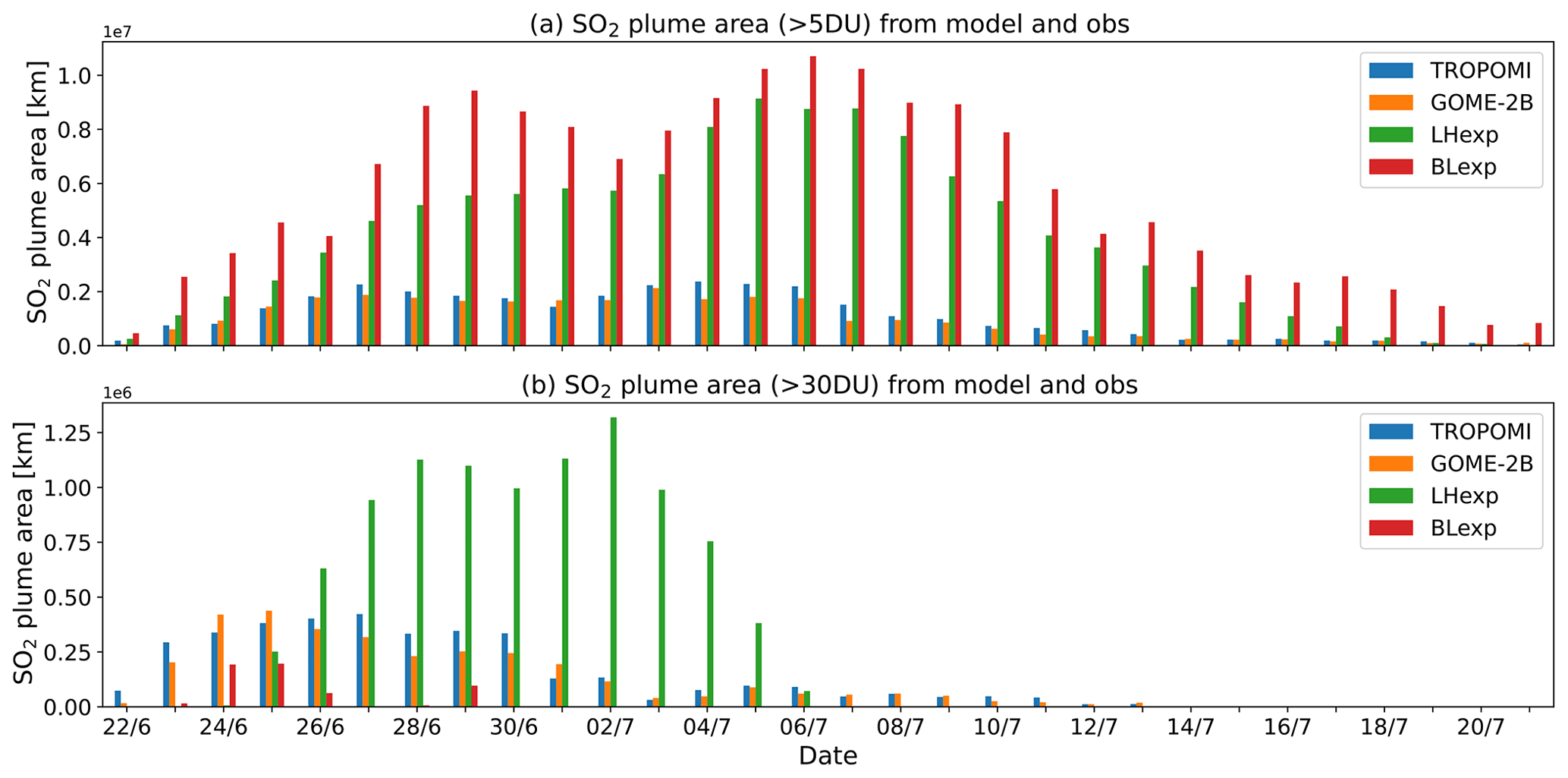
Figure 11SO2 plume area (in 1×10⁶ km2) from TROPOMI, GOME-2B, LHexp and BLexp TCSO2 analysis at 00:00 UTC for the Raikoke eruption (22 June to 21 July 2019). The values are calculated by gridding the data on a 1∘ × 1∘ grid and selecting the grid cells with TCSO2 values greater than (a) 5 DU and (b) 30 DU in the area 30–90∘ N.
Figure 10 shows the time series of the SO2 burden from NRT TROPOMI, GOME-2B and the two experiments calculated for threshold values of 5 DU and 30 DU, and Fig. 11 shows the corresponding time series of the plume areas. For the lower threshold of 5 DU, both the SO2 burden and the plume area are overestimated in LHexp and BLexp. This confirms what was already seen in Figs. 6 to 8, namely that the plumes are more spatially dispersed in the analysis than in the observations. The overestimation of the SO2 burden is larger in LHexp than in BLexp, with maximum values of 3 and 2 Tg, respectively, compared to 1.5 and 1.2 Tg for NRT TROPOMI and GOME-2B, respectively. However, the plume area is larger in BLexp, with a maximum extent of about 1 × 10⁷ km2, compared to 0.8 × 10⁷ km2 in LHexp and 0.2 × 10⁷ km2 calculated from the observations. The larger overestimation of the SO2 burden in LHexp is the result of differences in the background error standard deviation values used in the experiments and the fact that lower SO2 columns, which could correct an overestimation in parts of the plume, are not assimilated. BLexp fails to capture the higher SO2 column values, leading to an underestimation of plume area and SO2 burden for a threshold of 30 DU, while LHexp does have TCSO2 values > 30 DU but overestimates both plume area and SO2 burden.
To quantify the realism of the SO2 analyses and the quality of the SO2 forecasts, appropriate error measures need to be defined and used in addition to the visual inspection of the SO2 plumes. Statistical measures such as bias and root-mean-square error are not well suited because of the specific event character of the SO2 plumes. In addition to looking at the plume area and SO2 burden, we use threshold-based measures based on the number of hits (grid boxes where both model and observations detect the plume), misses (grid boxes where there is a plume in the observations but not in the model) or false alarms (grid boxes where the model has volcanic SO2 that is not seen in the observations) to quantify the error in the plume position. Flemming and Inness (2013) used hits and plume area measures for various thresholds. In this paper we combine the information about hits and misses and use as score the probability of detection (POD)
which lies between 0 and 1, with a value of 1 indicating a perfect score. We also us the critical success index (CSI), defined as
which additionally considers the number of false alarms and again has values between 0 and 1 with 1 indicating a perfect score (Nurmi, 2003). These are point-based comparisons and might score badly for features that are close but slightly misplaced between observations and model.
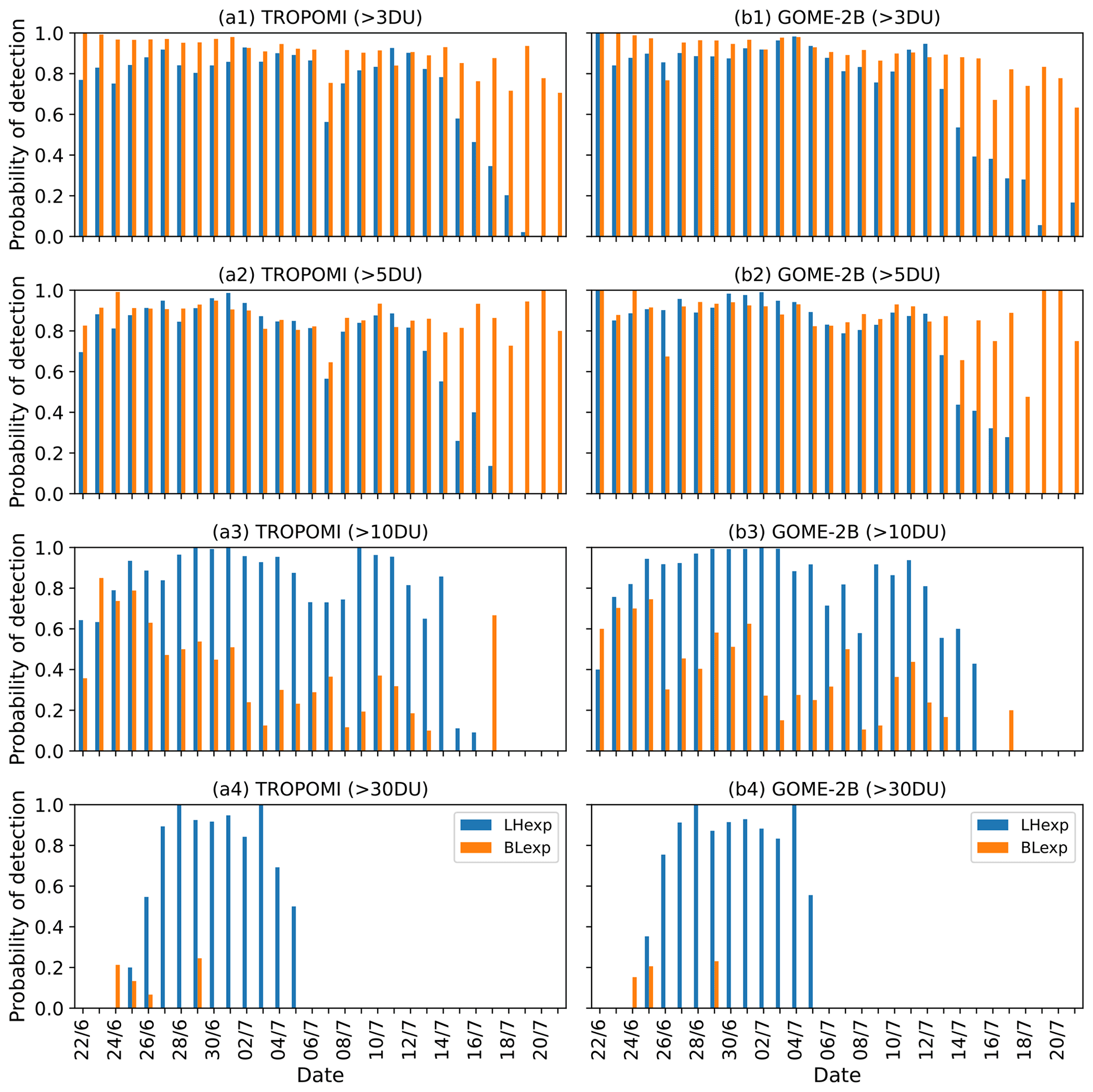
Figure 12Time series of POD for TCSO2 analysis fields (at 00:00 UTC) against (a) NRT TROPOMI and (b) GOME-2B for TCSO2 thresholds of (1) 3 DU, (2) 5 DU, (3) 10 DU and (4) 30 DU (22 June to 21 July 2019). Values for LHexp are shown in blue, and values for BLexp are shown in orange.
Figure 12 shows the POD from LHexp and BLexp for various TCSO2 analysis thresholds (3, 5, 10, 30 DU) scored against NRT TROPOMI and GOME-2B data. The results are very similar for both satellites. The parts of the plume with lower TCSO2 values are captured well by both experiments, with POD values above 0.9 for BLexp for most of the period and POD values above 0.8 for LHexp. The POD in LHexp decreases towards the end of the depicted period because the number of assimilated data drops strongly (see Fig. 8), while more observations are assimilated in BLexp at the later stage of the episode. BLexp, however, does not capture the higher values observed by NRT TROPOMI and GOME-2B well, while LHexp has a much higher POD for those parts of the plume. No values above 30 DU are detected after 5 July 2019.
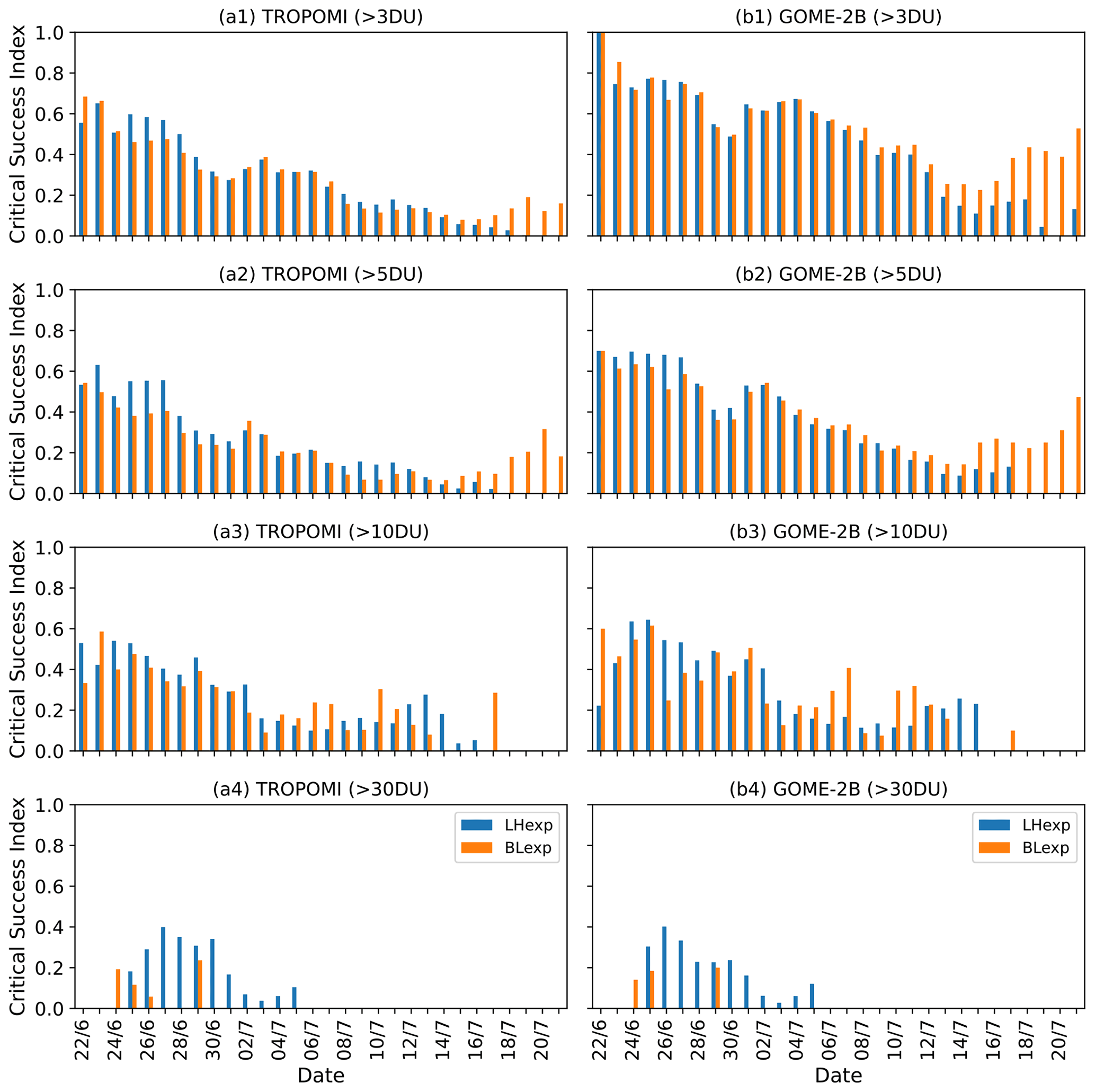
Figure 13Time series of CSI for TCSO2 analysis fields (at 00:00 UTC) against (a) NRT TROPOMI and (b) GOME-2B for TCSO2 thresholds of (1) 3 DU, (2) 5 DU, (3) 10 DU and (4) 30 DU (22 June to 21 July 2019). Values for LHexp are shown in blue, and values for BLexp are shown in orange.
Figure 13 shows the CSI from LHexp and BLexp, the measure that also penalizes the false alarms. As expected, these values are considerably lower than the POD (with maximum values around 0.6) because plume area and SO2 burden are overestimated in both experiments (see Fig. 9), leading to numerous false alarms. Both experiments behave similarly for the lower thresholds but TCSO2 values greater than 30 DU are again captured better in LHexp.
In summary, as far as the TCSO2 analysis fields are concerned, the performance of LHexp and BLexp is similar for TCSO2 columns below 10 DU, but BLexp does not capture the higher SO2 values as well as LHexp. Both experiments overestimate the SO2 burden and the plume area compared to the TROPOMI NRT and GOME-2B observations.

Figure 14Vertical cross sections along 60∘ N between 120 and 300∘ E showing the SO2 analysis field (in ppb) from (a) LHexp and (b) BLexp on 29 June 2019 at 00:00 UTC.
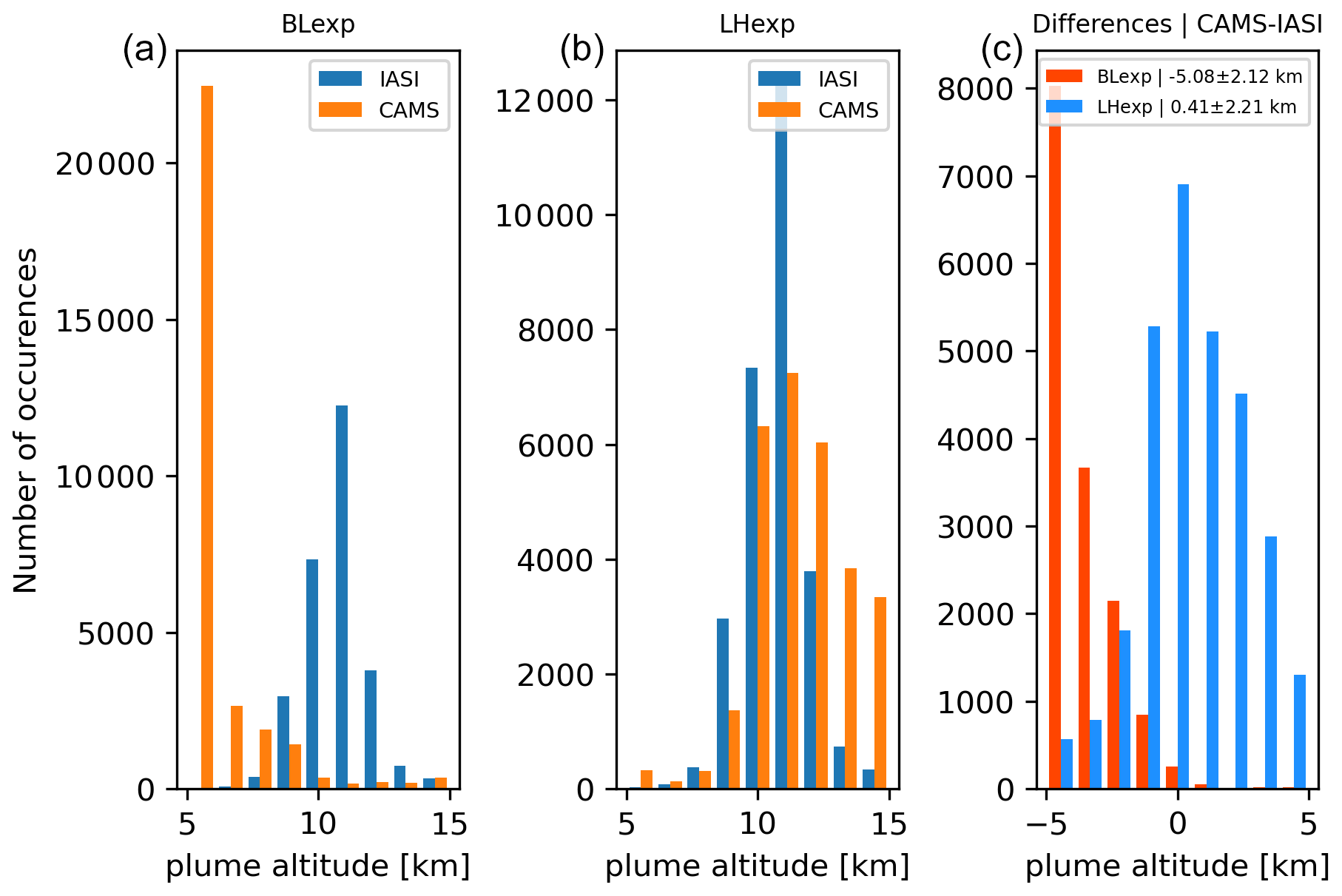
Figure 15Comparison of plume altitude from IASI ULB (Université libre de Bruxelles) LATMOS (Laboratoire Atmosphères, Observations Spatiales) data with the altitude of maximum SO2 concentration from LHexp (b) and BLexp (a) for the period 22–29 June 2019. Panel (c) shows a histogram of the differences in the plume altitudes (CAMS minus IASI) for LHexp (blue) and BLexp (red).
4.3.2 Vertical location of the SO2 plume
While the TCSO2 analyses from LHexp and BLexp score similarly in the detection of the TCSO2 plume observations by GOME-2B and NRT TROPOMI, at least for values less than 10 DU, the vertical distributions of the SO2 plumes from the experiments differ considerably. Figure 14 shows vertical cross sections along 60∘ N between 120–300∘ E through the SO2 plume on 29 June 2019 from LHexp and BLexp. The figure illustrates that the bulk of the SO2 plume is located between 200 and 100 hPa in LHexp, while it is located much lower, between 600 and 400 hPa, in BLexp. To assess which vertical distribution is more realistic, in Fig. 15 we compare the plume heights from the experiments with SO2 altitudes derived from IASI LATMOS ULB data (Clarisse et al., 2012) for the period 22 to 29 June 2019. The CAMS plume altitude was calculated as the altitude where the highest SO2 value was found in the CAMS SO2 profiles. The figure shows that the plume height in LHexp agrees well with the independent IASI plume altitude with a mean bias of 0.4 ± 2.2 km, while BLexp underestimates the plume altitude with a mean bias of −5.1 ± 2.1 km. Figure 15 illustrates that the altitude of the Raikoke SO2 plume in the CAMS analysis is considerably improved if SO2LH data are used rather than using the baseline configuration.
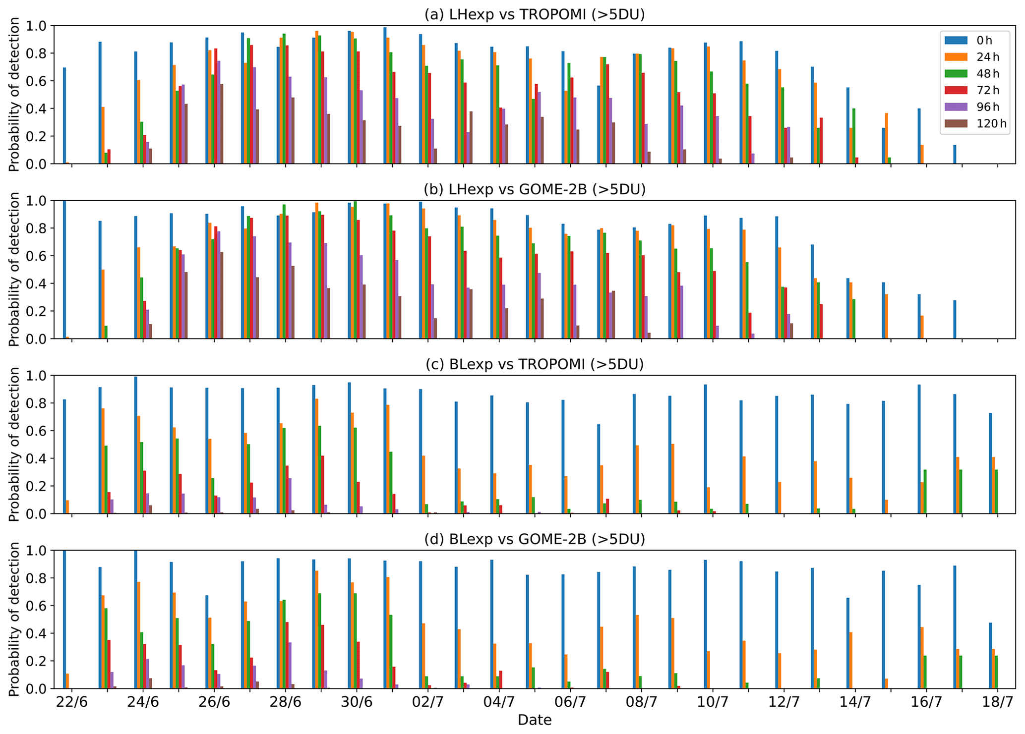
Figure 16Probability of detection of LHexp against (a) NRT TROPOMI and (b) GOME-2B and BLexp against (c) NRT TROPOMI and (d) GOME-2B for the period 22 June to 18 July 2021 for analysis at 00:00 UTC (blue), of a 24 h forecast (orange), of a 48 h forecast (green), of a 72 h forecast (red), of a 96 h forecast (purple) and of a 120 h forecast (brown).
4.3.3 Quality of the 5 d TCSO2 forecasts
Next, we assess the quality of the 5 d TCSO2 forecasts started from the LHexp and BLexp SO2 analyses. Figure 16 shows a time series of POD for a TCSO2 threshold of 5 DU from LHexp and BLexp for NRT TROPOMI and GOME-2B for the initial SO2 analysis and forecasts valid on the same day at different lead times (24 to 120 h). Figure 16 shows that the skill decreases with increasing forecast lead time in both experiments but that the degradation of skill with forecast lead time is considerably large in BLexp. For the 72 h forecasts LHexp has POD values between 0.6 and 0.8 and even the 96 h forecast still has values of 0.4. In contrast, BLexp only has POD values between 0.2 and 0.4 for the 72 h forecasts during June while values drop considerably during July when even the short 24 h forecasts from BLexp only have POD values between 0.2 and 0.4. In other words, in BLexp the skill of forecasting the location of the SO2 plumes seen by GOME-2B and the NRT TROPOMI 1 d in advance is similar to the skill of forecasting the SO2 plumes 4 d in advance in LHexp. The main reason for the lower forecast quality in BLexp is the fact that the SO2 plumes are located at the wrong altitude (see Fig. 15), and thus the prevailing winds will not transport the SO2 in the correct direction.
To further assess the forecast skill, we use the fractional skill score (FSS), which is a spatial comparison. It was originally used to assess the quality of precipitation forecasts (Roberts and Lean, 2008) but has more recently also been used to assess the skill of dispersion models to capture volcanic plumes (de Leeuw et al., 2021; Dacre et al., 2016; Harvey and Dacre, 2016). The FSS is calculated using the ratio of the modelled and observed fractional coverage of the SO2 plume at each location for various horizontal scales (neighbourhoods) and thresholds, and it assesses how the skill of the forecast varies depending on those parameters. To calculate it we grid the model TCSO2 analyses and forecasts at various lead times and the NRT TROPOMI and GOME-2B TCSO2 observations on a 1∘ × 1∘ grid and create binary fields for the chosen thresholds (in our case for TCSO2 > 1, 3, 5, 10, 20, 30 and 50 DU). Following this, for each grid point the fraction of surrounding grid points that exceed the threshold is calculated from the model field and the observations. To establish at which horizontal scale the SO2 analysis or forecast is useful we repeat this exercise with neighbourhoods of varying scales (i.e. 1, 3, 5∘, corresponding to neighbourhoods of 1, 9 and 25 grid boxes, respectively). An FSS of 1 means perfect alignment of the features in the observations and the model and an FSS of 0 a total mismatch. We use values of FSS greater than 0.5 to define a simulation that has some skill. This value was also used by de Leeuw et al. (2021) and Harvey and Dacre (2016). The FSS for a neighbourhood of length n is calculated following Roberts and Lean (2008) as
where MSE is the mean square error and MSE(n)=0 is a perfect forecast of a neighbourhood with length n. The reference MSE for each neighbourhood length n is given by
where i=1, Nx with Nx being the number of columns in the domain and j=1, Ny with Ny being the number of rows. M(n)i,j is the field of model fractions obtained from the model binary field for a square of length n, and O(n)i,j is the corresponding field of observed fractions. MSE(n)ref can be interpreted as the largest possible MSE that can be obtained from the model and observed fractions.
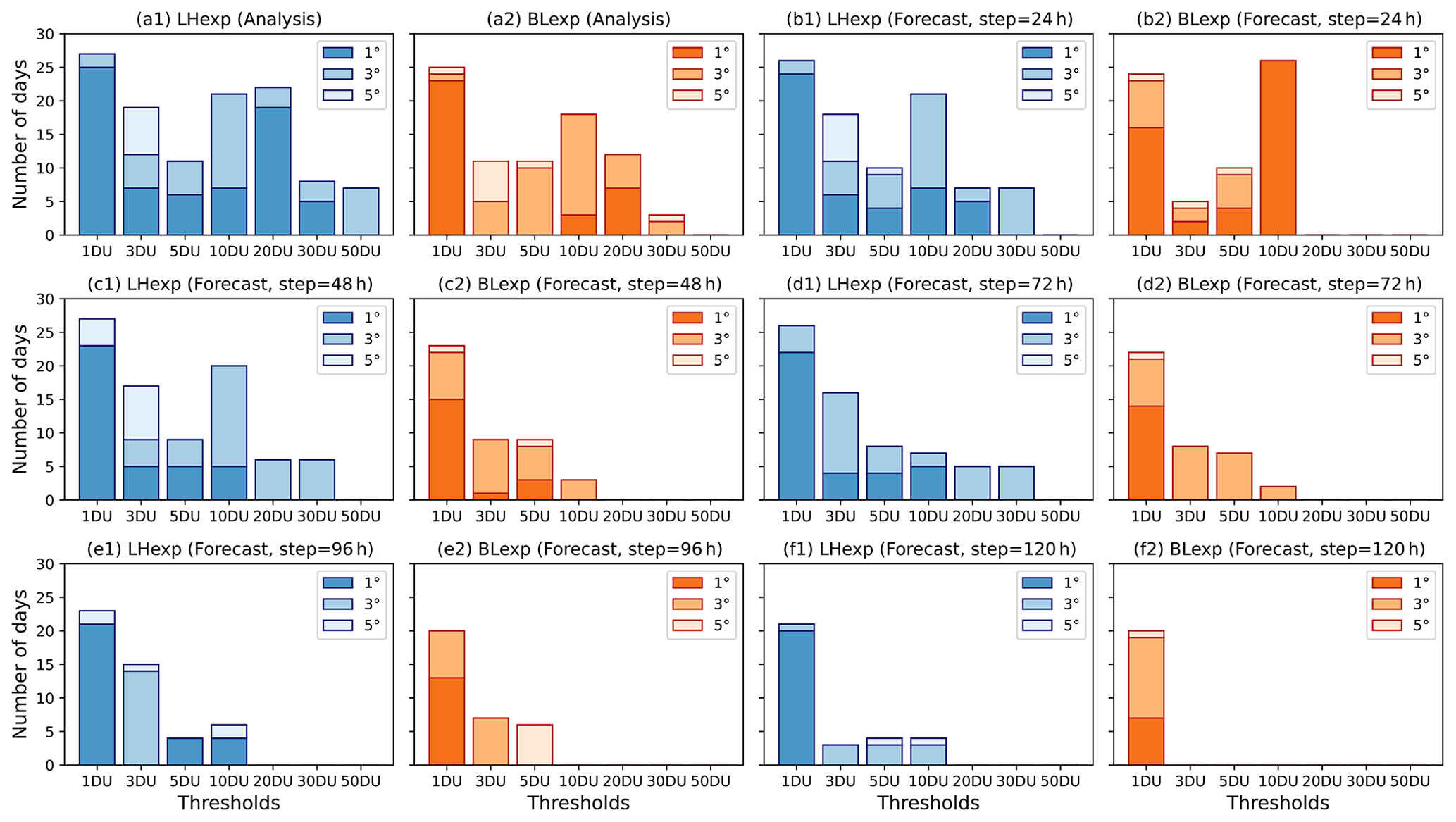
Figure 17Number of days since the eruption on 22 June 2019 that the LHexp (blue) and BLexp (orange) (a) analyses and forecasts at steps (b) 24, (c) 48, (d) 72, (e) 96 and (f) 120 h have some skill (FSS > 0.5) compared to NRT TROPOMI TCSO2 data for neighbourhood sizes of 1∘, 3∘ and 5∘ and thresholds of 1, 3, 5, 10, 20, 30 and 50 DU.
Figure 17 shows the number of days after the eruption that have FSS > 0.5 when comparing LHexp and BLexp with NRT TROPOMI data for the various thresholds to give some indication of a skill timescale, i.e. how long the analyses and the forecasts started from them can be considered as useful after the initial eruption. Also shown (in the lighter shadings) are the additional useful forecast days that are gained when the neighbourhood size is increased to 3∘ or 5∘. The main findings of the figure are that (1) the skill timescale is longer for the smaller thresholds, i.e. the overall shape of the plume is easier to reproduce than smaller-scale filaments with higher TCSO2 values, (2) the skill timescale drops with lead time, (3) the skill timescale increases if the neighbourhood size is increased, with a larger increase for higher thresholds, pointing to errors in the location of structures with higher TCSO2, which are reduced with a larger grid, and (4) the skill timescale is greater in LHexp than in BLexp, leading to better forecasts of the plume longer in advance, as already seen in Fig. 16.
We now look at the individual panels in more detail. Figure 17a shows the skill timescales of the TCSO2 analyses from LHexp and BLexp against NRT TROPOMI and illustrates that these give similarly useful TCSO2 fields (especially for the lower thresholds), as already seen in Sect. 4.3.1, but that the number of useful days is slightly larger in LHexp and that BLexp fails to capture the highest TCSO2 values. It is interesting to see the large number of days with FSS > 0.5 for the threshold of 20 DU in LHexp because this is the value below which no TCSO2 data are assimilated in LHexp. Figure 17b shows that the 24 h forecasts in LHexp have similar skill to the analysis, a skill timescale of 24 d for the 1 DU threshold and a neighbourhood size of 1∘, illustrating that the 24 h from the LHexp analysis can predict the overall location of the SO2 plume very well. For higher thresholds (> 30 DU) this drops to about 5 d after the eruption, and there is no skill for a threshold of 50 DU. The skill of the 48 and 72 h forecasts (Fig. 17c and d) are similar to that of the 24 h one for the thresholds up to 10 DU, but at a neighbourhood size of 1∘ the higher values (> 20 DU) have no skill anymore. As there is still skill on a 5 d timescale for these forecasts for a neighbourhood size of 3∘, this suggests that it is the location of the filaments with high TCSO2 values that is not correct rather than the forecast not maintaining any of the higher TCSO2 values. Even the 96 and 120 h forecasts (Fig. 17e and f) in LHexp have a skill timescale of slightly more than 20 d for the 1 DU threshold at 1∘, but the skill drops markedly for the higher thresholds, and for the 120 h forecasts skill is only found for thresholds up to 10 DU at 3∘ for up to 3 d after the eruption. Nevertheless, Fig. 17 shows that by assimilating SO2 LH data the CAMS system can predict the overall location of the SO2 plume up to 5 d in advance for about 20 d after the initial eruption. This corresponds to the time when the SO2 LH product does not detect volcanic SO2 anymore (see Fig. 8). Leeuw et al. (2021), using the Met Office's Numerical Atmospheric-dispersion Modelling Environment (NAME) dispersion model, found skill timescales of 12–17 d for low-density (> 1 DU) parts of the Raikoke SO2 cloud and shorter skill timescales of 2–4 d for the denser parts of the cloud (> 20 DU). It is interesting to see skill timescales of similar magnitudes to the ones obtained in our study even though their method is different. Leeuw et al. (2021) initialized the NAME dispersion model with eruption source parameters and then followed the evolution of the SO2 cloud, while we use data assimilation to update the location of the plume daily and provide daily forecasts with a maximum length of 5 d.
Figure 17 shows that the BLexp analysis has skill timescales similar to LHexp, confirming what was already seen in Figs. 12 and 13. Despite placing the SO2 cloud at the wrong altitude, the overall shape of the SO2 plume is still captured by the SO2 analysis. However, for higher thresholds the number of useful days after the eruption is smaller in BLexp, and the forecast skill drops more steeply with forecast lead time than in LHexp. There is no skill for the 24 h forecast at 1∘ for thresholds greater than 20 DU, and for the 48 h forecasts the skill timescale for a 1 DU threshold at 1∘ is 15 d, compared to 23 d in LHexp. The skill timescale remains around 14 d in BLexp for the 72 and 96 h forecasts for a 1 DU threshold at 1∘ and then drops to 6 d at 120 h. For the 72 to 120 h forecasts there is no skill for the higher thresholds for a neighbourhood size of 1∘, pointing to a worse misplacement of the smaller-scale features of the plume with higher TCSO2 values than in LHexp.
For GOME-2B (not shown) the number of useful forecast days is generally slightly lower, especially for a threshold of 1 DU, which might just be an artefact because GOME-2B does not detect so many volcanic pixels with low values. For thresholds of 3–30 DU the GOME-2 results for a neighbourhood size of 1∘ or 3∘ are very similar to the TROPOMI results for all the forecast ranges, with skill timescales of about 10 d for forecast lead times up to 72 h and around 5 d for the 96 h forecasts. Again, the performance of BLexp is worse than of LHexp and for the 48 h forecasts there is almost no skill in BLexp for the 1∘ neighbourhoods.
In this paper we document the procedure used to assimilate near real-time TCSO2 data from the TROPOMI and GOME-2 instruments in the operational CAMS NRT data assimilation system and explore the use of TROPOMI SO2 layer height data provided by the ESA-funded Sentinel-5P Innovation–SO2 Layer Height Project and produced with the Full-Physics Inverse Learning Machine algorithm (v3.1) developed by DLR. The assimilation of the FP_ILM SO2 LH data was tested for the 2019 Raikoke eruption and compared with results obtained when assimilating NRT TROPOMI TCSO2 data with the operational CAMS configuration.
While the operational CAMS approach of placing the SO2 increment in the mid-troposphere around 550 hPa gives surprisingly good results for the TCSO2 analyses and short-range forecasts in a lot of situations (including this case), the vertical distribution of SO2 in the baseline analysis is clearly wrong for the Raikoke eruption, which injected a copious amount of SO2 into the stratosphere. By using the FP_ILM TROPOMI SO2 LH data this can be much improved as the comparison with the independent SO2 plume heights retrieved from IASI shows. While the LH experiment agrees well with the IASI LATMOS ULB plume altitude products, with a mean bias of 0.4 ± 2.2 km, the baseline experiment underestimates the plume altitude with a mean bias of −5.1 ± 2.1 km. Consequently, the assimilation of the FP_ILM LH data leads to much improved SO2 forecasts and should improve the usefulness of the CAMS SO2 forecasts for users and also for the aviation industry.
In the baseline experiment the forecast skill drops much more for longer forecast lead times than in the LH experiment, which is seen when comparing point skill scores such as probability of detection and critical success index and when using the fractional skill score that also assesses spatial skill. Time series of the probability of detection score show that in the baseline experiment, the skill of forecasting the location of the Raikoke SO2 plume seen by GOME-2B and the NRT TROPOMI 1 d in advance is similar to the skill of forecasting the SO2 plume 4 d in advance in LHexp. The FSS shows that compared to NRT TROPOMI, even the 120 h forecasts of the LH experiment have a significant skill up to 20 d after the initial eruption for the prediction of TCSO2 for a 1 DU threshold and a neighbourhood size of 1∘, suggesting that the overall location of the SO2 plume is well reproduced. The skill is smaller for higher TCSO2 thresholds (about 5 d for forecast ranges up to 96 h on a 1∘ grid), illustrating that it is more difficult to accurately predict the location of areas with higher SO2 columns, which usually have smaller spatial scales. The skill timescale is shorter for the baseline experiment, with values around 15 d after the initial eruption for the 1 DU threshold for forecast ranges up to 96 h and 5 d for the 120 h forecasts, but there is no skill for any of the higher thresholds at a neighbourhood size of 1∘ from 72 h forecasts onwards. By assimilating FP_ILM SO2 LH data the CAMS system can predict the overall location of the Raikoke SO2 plume up to 5 d in advance for about 20 d after the initial eruption.
Our study also documents some issues of the CAMS TCSO2 assimilation approach, namely the overestimation of the SO2 burden and plume area by the data assimilation system, both in the operational configuration and when using the FP_ILM SO2 LH data. The main reason for this overestimation is the coarse horizontal resolution used in the minimizations (currently TL95 and TL159 in the operational CAMS system), which limits the wavenumbers that can be resolved in the wavelet formulation of the SO2 background errors. This in turn limits the horizontal correlation length scale that can be used for the SO2 background errors and that determines how far the increments from individual observations are spread out in the horizontal. In this paper we used TL159 and TL255 as the resolutions for the minimizations, but to properly resolve small-scale structures the resolutions of the minimizations would have to be even higher. Obviously, this would increase the numerical cost of running the minimization.
Other reasons that can contribute to an overestimation of the SO2 burden or plume area in the CAMS SO2 analysis could be the use of anthropogenic SO2 emissions in the CAMS model as the satellite data used for the comparisons are only the volcanic pixels. However, tests run without the anthropogenic emissions (not shown in this paper) did not show large differences compared to the experiments presented here, suggesting that this is not a big effect for the Raikoke eruption. Another possibility could be the fact that the satellite might miss a plume or part of a plume but that whole plume is present in the model. Finally, for the FP_ILM LH product the data are limited to TCSO2 > 20 DU (in v3.1), and lower values that might correct an overestimation from the previous analysis cycle are not used. In future we hope to also test the assimilation of IASI SO2 data with plume height information that would add extra information in the CAMS system.
One limitation in using the TROPOMI SO2 LH data is that the version used in this study (v3.1) only produces reliable information for TCSO2 > 20 DU, and thus most of the smaller volcanic eruptions that happen on a more regular basis than big explosive eruptions would be missed if only the FP_ILM TROPOMI SO2 LH data were assimilated in the CAMS NRT system. Improvements to the TROPOMI SO2 LH product are ongoing, and thus it should be possible to lower this limit in the future.
This study was based on the IFS model cycle 47R1. The ECWMF IFS code is only available subject to a licence agreement with ECMWF. ECMWF member state weather services and their approved partners will get granted access. The IFS code without modules for assimilation can be obtained for educational and academic purposes as part of the openIFS project (https://confluence.ecmwf.int/display/OIFS, ECMWF, 2022). A software licensing agreement with ECMWF is required to access the OpenIFS source distribution: despite the name it is not provided under any form of open-source software license. License agreements are free, limited to non-commercial use, forbid any real-time forecasting, and must be signed by research or educational organizations. Personal licenses are not provided. OpenIFS cannot be used to produce or disseminate real-time forecast products. ECMWF has limited resources to provide support and thus may temporarily cease issuing new licenses if it is deemed too difficult to provide a satisfactory level of support. Provision of an OpenIFS software license does not include access to ECMWF computers or data archives other than public datasets. A detailed documentation of the IFS code is available from https://www.ecmwf.int/en/publications/ifs-documentation (last access: 26 October 2021). The output from the assimilation experiments used in this study is available from https://apps.ecmwf.int/research-experiments/expver/ (last access: 26 October 2021) using the following DOIs for the six experiments:
-
hhu5 (Inness, 2021a): https://doi.org/10.21957/cygt-xf49;
-
hgze (Inness, 2021b): https://doi.org/10.21957/qfam-7474;
-
hhbu (Inness, 2021c): https://doi.org/10.21957/zpdt-f079;
-
hhtm (Inness, 2021d): https://doi.org/10.21957/jraa-s174;
-
hhtn (Inness, 2021e): https://doi.org/10.21957/ddxs-2v95;
-
hgz7 (Inness, 2021f): https://doi.org/10.21957/81bh-7h58.
The TROPOMI V3.1 SO2 LH data are available from https://doi.org/10.5281/zenodo.5602935 (Hedelt, 2021). The operational TROPOMI SO2 data are from the Copernicus Open Access Hub (https://scihub.copernicus.eu/, Copernicus Open Access Hub, 2022), and the IASI SO2 plume height data are from https://en.aeris-data.fr/ (AERIS, 2022).
AI prepared the code to assimilate the SO2 LH data, ran the analysis experiments, carried out most of the validation and wrote the paper. MA helped with the construction of the background error matrices. JF provided help with the modelling framework, and RR wrote the converter software to transfer the SO2 LH data from their native netcdf format to the BUFR format used in the ECMWF data assimilation system. MEK and DB performed the validation against the IASI/MetOp SO2 plume altitude data and provided Fig. 15. PH provided the SO2 LH data and developed the FP_ILM algorithm. DE and DL also contributed to the FP_ILM developments. All co-authors provided useful feedback on the paper.
The contact author has declared that neither they nor their co-authors have any competing interests.
Publisher's note: Copernicus Publications remains neutral with regard to jurisdictional claims in published maps and institutional affiliations.
The Copernicus Atmosphere Monitoring Service is operated by the European Centre for Medium-Range Weather Forecasts on behalf of the European Commission as part of the Copernicus Programme (http://copernicus.eu, last access: 30 January 2022), and CAMS data are freely available from https://atmosphere.copernicus.eu/data (last access: 30 January 2022). The SO2 analysis and forecast experiments used in this paper are available from https://apps.ecmwf.int/research-experiments/expver/ (last access: 30 January 2022) (see DOIs in Table 3). The FP_ILM TROPOMI SO2 LH product was developed in the framework of the ESA Sentinel-5p Innovation project. Maria-Elissavet Koukouli would like to acknowledge the use of the Aristotle University of Thessaloniki (AUTh) high-performance computing infrastructure and resources and the help of the AUTh IT Center. Maria-Elissavet Koukouli further acknowledges the use of the Atmospheric Toolbox®. IASI is a joint mission of EUMETSAT and the Centre National d'Etudes Spatiales (CNES, France). The authors acknowledge AERIS (https://en.aeris-data.fr/, last access: 30 January 2022) for providing access to the IASI SO2 plume height data used in this study and ULB-LATMOS for the development of the retrieval algorithms. Thanks to Anabel Bowen for improving Figs. 5 and 9.
This paper was edited by Graham Mann and reviewed by Nina Iren Kristiansen and one anonymous referee.
AERIS: IASI SO2 plume height data, https://en.aeris-data.fr/, last access: 30 January 2022.
Albert, M. F. M. A., Anguelova, M. D., Manders, A. M. M., Schaap, M., and de Leeuw, G.: Parameterization of oceanic whitecap fraction based on satellite observations, Atmos. Chem. Phys., 16, 13725–13751, https://doi.org/10.5194/acp-16-13725-2016, 2016.
Brenot, H., Theys, N., Clarisse, L., van Geffen, J., van Gent, J., Van Roozendael, M., van der A, R., Hurtmans, D., Coheur, P.-F., Clerbaux, C., Valks, P., Hedelt, P., Prata, F., Rasson, O., Sievers, K., and Zehner, C.: Support to Aviation Control Service (SACS): an online service for near-real-time satellite monitoring of volcanic plumes, Nat. Hazards Earth Syst. Sci., 14, 1099–1123, https://doi.org/10.5194/nhess-14-1099-2014, 2014.
Brenot, H., Theys, N., Clarisse, L., van Gent, J., Hurtmans, D. R., Vandenbussche, S., Papagiannopoulos, N., Mona, L., Virtanen, T., Uppstu, A., Sofiev, M., Bugliaro, L., Vázquez-Navarro, M., Hedelt, P., Parks, M. M., Barsotti, S., Coltelli, M., Moreland, W., Scollo, S., Salerno, G., Arnold-Arias, D., Hirtl, M., Peltonen, T., Lahtinen, J., Sievers, K., Lipok, F., Rüfenacht, R., Haefele, A., Hervo, M., Wagenaar, S., Som de Cerff, W., de Laat, J., Apituley, A., Stammes, P., Laffineur, Q., Delcloo, A., Lennart, R., Rokitansky, C.-H., Vargas, A., Kerschbaum, M., Resch, C., Zopp, R., Plu, M., Peuch, V.-H., Van Roozendael, M., and Wotawa, G.: EUNADICS-AV early warning system dedicated to supporting aviation in the case of a crisis from natural airborne hazards and radionuclide clouds, Nat. Hazards Earth Syst. Sci., 21, 3367–3405, https://doi.org/10.5194/nhess-21-3367-2021, 2021.
Carn, S. A., Clarisse, L., and Prata, A. J.: Multi-decadal Satellite Measurements of Global Volcanic Degassing, J. Volcanol. Geoth. Res., 311, 99–134. https://doi.org/10.1016/j.jvolgeores.2016.01.002, 2016.
Clarisse, L., Hurtmans, D., Clerbaux, C., Hadji-Lazaro, J., Ngadi, Y., and Coheur, P.-F.: Retrieval of sulphur dioxide from the infrared atmospheric sounding interferometer (IASI), Atmos. Meas. Tech., 5, 581–594, https://doi.org/10.5194/amt-5-581-2012, 2012.
Clarisse, L., Coheur, P.-F., Theys, N., Hurtmans, D., and Clerbaux, C.: The 2011 Nabro eruption, a SO2 plume height analysis using IASI measurements, Atmos. Chem. Phys., 14, 3095–3111, https://doi.org/10.5194/acp-14-3095-2014, 2014.
Clerbaux, C., Hadji-Lazaro, J., Turquety, S., George, M., Boynard, A., Pommier, M., Safieddine, S., Coheur, P.-F., Hurtmans, D., Clarisse, L., and M. Van Damme: Tracking pollutants from space: Eight years of IASI satellite observation, C. R. Geosci., 347, 134–144, https://doi.org/10.1016/j.crte.2015.06.001, 2015.
Copernicus Open Access Hub: TROPOMI, https://scihub.copernicus.eu/, last access: 30 January 2022.
Courtier, P., Thépaut, J.-N., and Hollingsworth, A.: A strategy for operational implementation of 4D-Var, using an incremental approach, Q. J. Roy. Meteor. Soc., 120, 1367–1388, 1994.
Dacre, H. F., Grant, A. L. M., Hogan, R. J. , Belcher, S. E., Thomson, D. J., Devenish, B. J., Marenco, F., Hort, M. C., Haywood, J. M., Ansmann, A., Mattis, I., and Clarisse, L.: Evaluating the structure and magnitude of the ash plume during the initial phase of the 2010 Eyjafjallajokull eruption using lidar observations and NAME simulations, J. Geophys. Res., 116, D00U03, https://doi.org/10.1029/2011JD015608, 2011.
Dacre, H. F., Harvey, N. J., Webley, P. W., and Morton, D.: How accurate are volcanic ash simulations of the 2010 Eyjafjallajökul eruption?, J. Geophys. Res. Atmos., 121, 3534–3547, https://doi.org/10.1002/2015JD024265, 2016.
de Leeuw, J., Schmidt, A., Witham, C. S., Theys, N., Taylor, I. A., Grainger, R. G., Pope, R. J., Haywood, J., Osborne, M., and Kristiansen, N. I.: The 2019 Raikoke volcanic eruption – Part 1: Dispersion model simulations and satellite retrievals of volcanic sulfur dioxide, Atmos. Chem. Phys., 21, 10851–10879, https://doi.org/10.5194/acp-21-10851-2021, 2021.
Diamantakis, M. and Flemming, J.: Global mass fixer algorithms for conservative tracer transport in the ECMWF model, Geosci. Model Dev., 7, 965–979, https://doi.org/10.5194/gmd-7-965-2014, 2014.
ECMWF: openIFS project, https://confluence.ecmwf.int/display/OIFS, last access: 30 January 2022.
Efremenko, D. S., Loyola R., D. G., Hedelt, P., and Spurr, R. J. D.: Volcanic SO2 plume height retrieval from UV sensors using a full-physics inverse learning machine algorithm, Int. J. Remote Sens., 38, 1–27, https://doi.org/10.1080/01431161.2017.1348644, 2017.
Fedkin, N. M., Li, C., Krotkov, N. A., Hedelt, P., Loyola, D. G., Dickerson, R. R., and Spurr, R.: Volcanic SO2 effective layer height retrieval for the Ozone Monitoring Instrument (OMI) using a machine-learning approach, Atmos. Meas. Tech., 14, 3673–3691, https://doi.org/10.5194/amt-14-3673-2021, 2021.
Fisher, M.: Generalized frames on the sphere with application to background error covariance modelling, Seminar on resent developments in numerical methods for atmospheric and ocean modelling, 6–10 September 2004, Proceedings, ECMWF, pp. 87–101, available from ECMWF, Shinfield Park, Reading, Berkshire, RG2 9AX, UK, 2004.
Fisher, M.: Wavelet Jb – A new way to model the statistics of back-ground errors, ECMWF Newsletter, 106, 23–28, available from ECMWF, Shinfield Park, Reading, Berkshire, RG2 9AX, UK, 2006.
Fisher, M. and Andersson, E.: Developments in 4D-Var and Kalman Filtering, ECMWF Technical Memorandum 347, available from ECMWF, Shinfield Park, Reading, Berkshire, RG2 9AX, UK, https://www.ecmwf.int/sites/default/files/elibrary/2001/9409-developments-4d-var-and-kalman-filtering.pdf (last access: 30 January 2022), 2001.
Flemming, J., and Inness, A.: Volcanic sulfur dioxide plume forecasts based on UV satellite retrievals for the 2011 Grímsvötn and the 2010 Eyjafjallajökull eruption, J. Geophys. Res.-Atmos., 118, 10172–10189, https://doi.org/10.1002/jgrd.50753, 2013.
Flemming, J., Huijnen, V., Arteta, J., Bechtold, P., Beljaars, A., Blechschmidt, A.-M., Diamantakis, M., Engelen, R. J., Gaudel, A., Inness, A., Jones, L., Josse, B., Katragkou, E., Marecal, V., Peuch, V.-H., Richter, A., Schultz, M. G., Stein, O., and Tsikerdekis, A.: Tropospheric chemistry in the Integrated Forecasting System of ECMWF, Geosci. Model Dev., 8, 975–1003, https://doi.org/10.5194/gmd-8-975-2015, 2015.
Flemming, J., Benedetti, A., Inness, A., Engelen, R. J., Jones, L., Huijnen, V., Remy, S., Parrington, M., Suttie, M., Bozzo, A., Peuch, V.-H., Akritidis, D., and Katragkou, E.: The CAMS interim Reanalysis of Carbon Monoxide, Ozone and Aerosol for 2003–2015, Atmos. Chem. Phys., 17, 1945–1983, https://doi.org/10.5194/acp-17-1945-2017, 2017.
Goitom, B., Oppenheimer, C., Hammond, J. O. S., Grandin, R., Barnie, T., Donovan, A., Ogubazghi, G., Yohannes, E., Kibrom, G., Kendall, J.-M., Carn, S. A, Fee, D., Sealing, C., Keir, D., Ayele, A., Blundy, J., Hamlyn, J., Wright, T., and Berhe, S.: First recorded eruption of Nabro volcano, Eritrea, 2011, B. Volcanol., 77, 85, https://doi.org/10.1007/s00445-015-0966-3, 2015.
Granier, C., Darras, S., Denier van der Gon, H., Doubalova, J., Elguindi, N., Galle, B., Gauss, M., Guevara, M., Jalkanen, J.-P., Kuenen, J., Liousse, C., Quack, B., Simpson, D., and Sindelarova, K.: The Copernicus Atmosphere Monitoring Service global and regional emissions (April 2019 version), Copernicus Atmosphere Monitoring Service (CAMS) report, https://doi.org/10.24380/d0bn-kx16, 2019.
Grebennikov, V. S., Zubachev, D. S., Korshunov, V. A., Sakhibgareev, D. G., and Chernikh, I. A.: Observations of Stratospheric Aerosol at Rosgidromet Lidar Stations after the Eruption of the Raikoke Volcano in June 2019, Atmos. Ocean. Opt., 33, 519–523, https://doi.org/10.1134/S1024856020050097, 2020.
Harvey, N. J. and Dacre, H. F.: Spatial evaluation of volcanic ash forecasts using satellite observations, Atmos. Chem. Phys., 16, 861–872, https://doi.org/10.5194/acp-16-861-2016, 2016.
Hedelt, P.: Sentinel-5p/TROPOMI SO2 Layer Height dataset covering the Raikoke volcanic eruption 2019 (3.1), Zenodo [data set], https://doi.org/10.5281/zenodo.5602935, 2021.
Hedelt, P., Efremenko, D. S., Loyola, D. G., Spurr, R., and Clarisse, L.: Sulfur dioxide layer height retrieval from Sentinel-5 Precursor/TROPOMI using FP_ILM, Atmos. Meas. Tech., 12, 5503–5517, https://doi.org/10.5194/amt-12-5503-2019, 2019.
Huijnen, V., Williams, J., van Weele, M., van Noije, T., Krol, M., Dentener, F., Segers, A., Houweling, S., Peters, W., de Laat, J., Boersma, F., Bergamaschi, P., van Velthoven, P., Le Sager, P., Eskes, H., Alkemade, F., Scheele, R., Nédélec, P., and Pätz, H.-W.: The global chemistry transport model TM5: description and evaluation of the tropospheric chemistry version 3.0, Geosci. Model Dev., 3, 445–473, https://doi.org/10.5194/gmd-3-445-2010, 2010.
Huijnen, V., Pozzer, A., Arteta, J., Brasseur, G., Bouarar, I., Chabrillat, S., Christophe, Y., Doumbia, T., Flemming, J., Guth, J., Josse, B., Karydis, V. A., Marécal, V., and Pelletier, S.: Quantifying uncertainties due to chemistry modelling – evaluation of tropospheric composition simulations in the CAMS model (cycle 43R1), Geosci. Model Dev., 12, 1725–1752, https://doi.org/10.5194/gmd-12-1725-2019, 2019.
Inness, A.: Model data exp=hhu5 for research article “Evaluating the assimilation of S5P/TROPOMI near real-time SO2 columns and layer height data into the CAMS integrated forecasting system (CY47R1), based on a case study of the 2019 Raikoke eruption”, ECMWF [data set], https://doi.org/10.21957/cygt-xf49, 2021a.
Inness, A.: Model data exp=hgze for research article “Evaluating the assimilation of S5P/TROPOMI near real-time SO2 columns and layer height data into the CAMS integrated forecasting system (CY47R1), based on a case study of the 2019 Raikoke eruption”, ECMWF [data set], https://doi.org/10.21957/qfam-7474, 2021b.
Inness, A.: Model data exp=hhbu for research article “Evaluating the assimilation of S5P/TROPOMI near real-time SO2 columns and layer height data into the CAMS integrated forecasting system (CY47R1), based on a case study of the 2019 Raikoke eruption”, ECMWF [data set], https://doi.org/10.21957/zpdt-f079, 2021c.
Inness, A.: Model data exp=hhtm for research article “Evaluating the assimilation of S5P/TROPOMI near real-time SO2 columns and layer height data into the CAMS integrated forecasting system (CY47R1), based on a case study of the 2019 Raikoke eruption”, ECMWF [data set], https://doi.org/10.21957/jraa-s174 , 2021d.
Inness, A.: Model data exp=hhtn for research article “Evaluating the assimilation of S5P/TROPOMI near real-time SO2 columns and layer height data into the CAMS integrated forecasting system (CY47R1), based on a case study of the 2019 Raikoke eruption”, ECMWF [data set], https://doi.org/10.21957/ddxs-2v95, 2021e.
Inness, A.: Model data exp=hgz7 for research article “Evaluating the assimilation of S5P/TROPOMI near real-time SO2 columns and layer height data into the CAMS integrated forecasting system (CY47R1), based on a case study of the 2019 Raikoke eruption”, ECMWF [data set], https://doi.org/10.21957/81bh-7h58, 2021f.
Inness, A., Blechschmidt, A.-M., Bouarar, I., Chabrillat, S., Crepulja, M., Engelen, R. J., Eskes, H., Flemming, J., Gaudel, A., Hendrick, F., Huijnen, V., Jones, L., Kapsomenakis, J., Katragkou, E., Keppens, A., Langerock, B., de Mazière, M., Melas, D., Parrington, M., Peuch, V. H., Razinger, M., Richter, A., Schultz, M. G., Suttie, M., Thouret, V., Vrekoussis, M., Wagner, A., and Zerefos, C.: Data assimilation of satellite-retrieved ozone, carbon monoxide and nitrogen dioxide with ECMWF's Composition-IFS, Atmos. Chem. Phys., 15, 5275–5303, https://doi.org/10.5194/acp-15-5275-2015, 2015.
Inness, A., Ades, M., Agustí-Panareda, A., Barré, J., Benedictow, A., Blechschmidt, A.-M., Dominguez, J. J., Engelen, R., Eskes, H., Flemming, J., Huijnen, V., Jones, L., Kipling, Z., Massart, S., Parrington, M., Peuch, V.-H., Razinger, M., Remy, S., Schulz, M., and Suttie, M.: The CAMS reanalysis of atmospheric composition, Atmos. Chem. Phys., 19, 3515–3556, https://doi.org/10.5194/acp-19-3515-2019, 2019.
Koukouli, M.-E., Michailidis, K., Hedelt, P., Taylor, I. A., Inness, A., Clarisse, L., Balis, D., Efremenko, D., Loyola, D., Grainger, R. G., and Retscher, C.: Volcanic SO2 Layer Height by TROPOMI/S5P; validation against IASI/MetOp and CALIOP/CALIPSO observations, Atmos. Chem. Phys. Discuss. [preprint], https://doi.org/10.5194/acp-2021-936, in review, 2021.
Laloyaux, P., Bonavita, M., Chrust, M., and Gürol, S.: Exploring the potential and limitations of weak-constraint 4D-Var, Q. J. Roy. Meteor. Soc., 146, 4067–4082, https://doi.org/10.1002/qj.3891, 2020.
Loyola, D. G., Xu, J., Heue, K.-P., and Zimmer, W.: Applying FP_ILM to the retrieval of geometry-dependent effective Lambertian equivalent reflectivity (GE_LER) daily maps from UVN satellite measurements, Atmos. Meas. Tech., 13, 985–999, https://doi.org/10.5194/amt-13-985-2020, 2020.
Moxnes, E. D., Kristiansen, N. I., Stohl, A., Clarisse, L., Durant, A., Weber, K., and Vogel, A.: Separation of ash and sulfur dioxide during the 2011 Grímsvötn eruption, J. Geophys. Res.-Atmos., 119, 7477–7501, https://doi.org/10.1002/2013JD021129, 2014.
Munro, R., Lang, R., Klaes, D., Poli, G., Retscher, C., Lindstrot, R., Huckle, R., Lacan, A., Grzegorski, M., Holdak, A., Kokhanovsky, A., Livschitz, J., and Eisinger, M.: The GOME-2 instrument on the Metop series of satellites: instrument design, calibration, and level 1 data processing – an overview, Atmos. Meas. Tech., 9, 1279–1301, https://doi.org/10.5194/amt-9-1279-2016, 2016.
Muser, L. O., Hoshyaripour, G. A., Bruckert, J., Horváth, Á., Malinina, E., Wallis, S., Prata, F. J., Rozanov, A., von Savigny, C., Vogel, H., and Vogel, B.: Particle aging and aerosol–radiation interaction affect volcanic plume dispersion: evidence from the Raikoke 2019 eruption, Atmos. Chem. Phys., 20, 15015–15036, https://doi.org/10.5194/acp-20-15015-2020, 2020.
Nurmi, P.: Recommendations on the verification of local weather forecasts, ECMWF Techical Memorandum, no. 430, https://www.ecmwf.int/node/11401 (last access: 30 January 2022), 2003.
Parrish, D. F. and Derber, J. C.: The National Meteorological Center's spectral statistical-interpolation analysis scheme, Mon. Weather Rev., 120, 1747–1763, 1992.
Platt, U.: Air Monitoring by Differential Optical Absorption Spectroscopy, in: Encyclopedia of Analytical Chemistry, edited by: Meyers, R. A., Wiley Online Library, https://doi.org/10.1002/9780470027318.a0706.pub2, 2017.
Platt, U. and Stutz, J.: Differential Optical Absorption Spectroscopy (DOAS): Principle and Applications, Springer, Berlin, 2008.
Prata, A. T., Dacre, H. F., Irvine, E. A., Mathieu, E, Shine, K. P., and Clarkson, R. J.: Calculating and communicating ensemble-based volcanic ash dosage and concentration risk for aviation, Meteorol. Appl., 26, 253–266, https://doi.org/10.1002/met.1759, 2019.
Prata, F., Woodhouse, M., Huppert, H. E., Prata, A., Thordarson, T., and Carn, S.: Atmospheric processes affecting the separation of volcanic ash and SO2 in volcanic eruptions: inferences from the May 2011 Grímsvötn eruption, Atmos. Chem. Phys., 17, 10709–10732, https://doi.org/10.5194/acp-17-10709-2017, 2017.
Puķīte, J., Kühl, S., Deutschmann, T., Platt, U., and Wagner, T.: Extending differential optical absorption spectroscopy for limb measurements in the UV, Atmos. Meas. Tech., 3, 631–653, https://doi.org/10.5194/amt-3-631-2010, 2010.
Rémy, S., Kipling, Z., Flemming, J., Boucher, O., Nabat, P., Michou, M., Bozzo, A., Ades, M., Huijnen, V., Benedetti, A., Engelen, R., Peuch, V.-H., and Morcrette, J.-J.: Description and evaluation of the tropospheric aerosol scheme in the European Centre for Medium-Range Weather Forecasts (ECMWF) Integrated Forecasting System (IFS-AER, cycle 45R1), Geosci. Model Dev., 12, 4627–4659, https://doi.org/10.5194/gmd-12-4627-2019, 2019.
Rix, M., Valks, P., Hao, N., Loyola, D., Schlager, H., Huntrieser, H., Flemming, J., Koehler, U., Schumann, U., and Inness, A.: Volcanic SO2, BrO and plume height estimations using GOME-2 satellite measurements during the eruption of Eyjafjallajökull in May 2010, J. Geophys. Res.-Atmos., 117, D00U19, https://doi.org/10.1029/2011JD016718, 2012.
Schmidt, A., Roberts, N. M., and Lean, H. W.: Assessing hazards to aviation from sulfur dioxide emitted by explosive Icelandic eruptions, J. Geophys. Res.-Atmos., 119, 14180–14196, https://doi.org/10.1002/2014JD022070, 2014.
Stohl, A., Prata, A. J., Eckhardt, S., Clarisse, L., Durant, A., Henne, S., Kristiansen, N. I., Minikin, A., Schumann, U., Seibert, P., Stebel, K., Thomas, H. E., Thorsteinsson, T., Tørseth, K., and Weinzierl, B.: Determination of time- and height-resolved volcanic ash emissions and their use for quantitative ash dispersion modeling: the 2010 Eyjafjallajökull eruption, Atmos. Chem. Phys., 11, 4333–4351, https://doi.org/10.5194/acp-11-4333-2011, 2011.
Theys, N., De Smedt, I., Yu, H., Danckaert, T., van Gent, J., Hörmann, C., Wagner, T., Hedelt, P., Bauer, H., Romahn, F., Pedergnana, M., Loyola, D., and Van Roozendael, M.: Sulfur dioxide retrievals from TROPOMI onboard Sentinel-5 Precursor: algorithm theoretical basis, Atmos. Meas. Tech., 10, 119–153, https://doi.org/10.5194/amt-10-119-2017, 2017.
Thomas, H. E. and Prata, A. J.: Sulphur dioxide as a volcanic ash proxy during the April–May 2010 eruption of Eyjafjallajökull Volcano, Iceland, Atmos. Chem. Phys., 11, 6871–6880, https://doi.org/10.5194/acp-11-6871-2011, 2011.
Tournigand, P.-Y., Cigala, V., Lasota, E., Hammouti, M., Clarisse, L., Brenot, H., Prata, F., Kirchengast, G., Steiner, A. K., and Biondi, R.: A multi-sensor satellite-based archive of the largest SO2 volcanic eruptions since 2006, Earth Syst. Sci. Data, 12, 3139–3159, https://doi.org/10.5194/essd-12-3139-2020, 2020.
Vaughan, G., Wareing, D., and Ricketts, H.: Measurement Report: Lidar measurements of stratospheric aerosol following the 2019 Raikoke and Ulawun volcanic eruptions, Atmos. Chem. Phys., 21, 5597–5604, https://doi.org/10.5194/acp-21-5597-2021, 2021.
Xu, J., Schüssler, O., Loyola Rodriguez, D. G., Romahn, F., and Doicu, A.: A novel ozone profile shape retrieval using Full-Physics Inverse Learning Machine (FP-ILM), IEEE J. Sel. Topics Appl. Earth Observ. Remote Sens., 10, 5442–5457, https://doi.org/10.1109/JSTARS.2017.2740168, 2017.
Yarwood, G., Rao, S., Yocke, M., and Whitten, G.: Updates to the carbon bond chemical mechanism: CB05, Final report to the US EPA, EPA Report Number: RT-0400675, CAMx, http://www.camx.com (last access: 30 January 2022), 2005.
Zhu, Y., Toon, O. B., Jensen, E. J., Bardeen, C. G., Mills, M. J., Tolbert, M. A., Yu, P., and Woods, S.: Persisting volcanic ash particles impact stratospheric SO2 lifetime and aerosol optical properties, Nat. Commun., 11, 4526, https://doi.org/10.1038/s41467-020-18352-5, 2020.