Temperature forecasting by deep learning methods

Numerical weather prediction (NWP) models solve a system of partial differential equations based on physical laws to forecast the future state of the atmosphere. These models are deployed operationally, but they are computationally very expensive. Recently, the potential of deep neural networks to generate bespoke weather forecasts has been explored in a couple of scientific studies inspired by the success of video frame prediction models in computer vision. In this study, a simple recurrent neural network with convolutional filters, called ConvLSTM, and an advanced generative network, the Stochastic Adversarial Video Prediction (SAVP) model, are applied to create hourly forecasts of the 2 m temperature for the next 12 h over Europe. We make use of 13 years of data from the ERA5 reanalysis, of which 11 years are utilized for training and 1 year each is used for validating and testing. We choose the 2 m temperature, total cloud cover, and the 850 hPa temperature as predictors and show that both models attain predictive skill by outperforming persistence forecasts. SAVP is superior to ConvLSTM in terms of several evaluation metrics, confirming previous results from computer vision that larger, more complex networks are better suited to learn complex features and to generate better predictions. The 12 h forecasts of SAVP attain a mean squared error (MSE) of about 2.3 K², an anomaly correlation coefficient (ACC) larger than 0.85, a structural similarity index (SSIM) of around 0.72, and a gradient ratio (r_G) of about 0.82. The ConvLSTM yields a higher MSE (3.6 K²), a smaller ACC (0.80) and SSIM (0.65), and a slightly larger r_G (0.84). The superior performance of SAVP in terms of MSE, ACC, and SSIM can be largely attributed to the generator. A sensitivity study shows that a larger weight of the generative adversarial network (GAN) component in the SAVP loss leads to even better preservation of spatial variability at the cost of a somewhat increased MSE (2.5 K²). Including the 850 hPa temperature as an additional predictor enhances the forecast quality, and the model also benefits from a larger spatial domain. By contrast, adding the total cloud cover as predictor or reducing the amount of training data to 8 years has only small effects. Although the temperature forecasts obtained in this way are still less powerful than contemporary NWP models, this study demonstrates that sophisticated deep neural networks may achieve considerable forecast quality beyond the nowcasting range in a purely data-driven way.

1 Introduction

Accurate predictions of weather are important for many aspects of modern society. They are of high relevance in economy and industry, e.g. for agriculture, for the (renewable) electric power industry, or for prevention against natural hazards. Since the early 1960s, numerical weather prediction (NWP) models are run operationally at meteorological centres all over the world. These models are nowadays capable of simulating the dynamics of the global atmosphere down to the kilometre scale (Bauer et al., 2015). While their predictions have reached a remarkable degree of reliability, the required computational resources are enormous (Zaengl et al., 2015).

Over recent years, deep learning (DL) has been successfully applied in computer vision applications, such as self-driving cars (Rao and Frtunikj, 2018), human action prediction (Kong and Fu, 2018), and anomaly detection (Liu et al., 2018). These show that deep neural networks have the ability to recognize complex patterns and uncover highly non-linear relations in a data-driven way. Thus, hopes are raised that deep learning can be used for weather prediction and Earth system science (Schultz et al., 2021), which have to deal with many complex, multi-scale, and non-linear coupled processes (Orlanski, 1975). The weather and climate communities are beginning to investigate the use of these advanced machine learning (ML) methods in the context of weather (McGovern et al., 2017) and climate forecasting (Reichstein et al., 2019), such as data assimilation (e.g. Hatfield et al., 2021), emulation of physical parameterization (e.g. Han et al., 2020), and detection of extreme weather events in climate datasets (e.g. Racah et al., 2016).

As discussed in Schultz et al. (2021), there are many potential applications of DL in the field of weather forecasting. DL methods can be integrated in each step of the NWP workflow, which comprises preprocessing of observational data, assimilation of these data into the modelled real atmospheric state, forecasting with a numerical model, and post-processing on the raw model outputs (see Fig. 1 in Schultz et al., 2021). Here, we provide a proof-of-concept study on replacing the NWP model with data-driven video prediction methods to forecast the evolution of the atmospheric state, particularly the 2 m temperature, up to 12 h ahead. This is considerably longer than the typical range of nowcasting applications with a lead time of 3 h or less (Wilson et al., 2010) but shorter than medium-range forecasts targeted in other studies (cf. Scher, 2018; Rasp and Lerch, 2018; Weyn et al., 2020). Together with an hourly temporal resolution of the video prediction model which aligns with the temporal resolution of operational NWP model output, our application focuses on predicting the diurnal cycle of 2 m temperature. This approach comprises two potential challenges for deep neural networks: a quick error accumulation in an autoregressive forecast task (see, e.g. Rasp et al., 2020; Scher and Messori, 2019) and the prediction of quasi-periodic processes for which deep neural networks are known to struggle with (Ziyin et al., 2020).

Weather forecasting shares some similarities with video prediction by deep learning. Both explore spatio-temporal patterns from previously observed data to generate a plausible future state of the system. Nevertheless, there are at least two main differences. First, video prediction is mostly used for human pose, physical object, and trajectory forecasting, where individual objects are often clearly separable from the background and do not interact with each other on several spatio-temporal scales. Temporal patterns are learned from the movement of objects to then generate a series of frames anticipating how a scene might evolve during the next few seconds. In contrast, weather data do not contain clearly separable objects and the physical laws governing the evolution of weather patterns over time are much more complex due to multi-scale interactions (see, e.g., Orlanski, 1975). For instance, a convective system is driven by large-scale flow patterns (e.g. embedded in a synoptic-scale low) and is subject to turbulence processes in the planetary boundary layer (e.g. convection triggering). Vice versa, the convection itself vents the planetary boundary layer and also modifies the large-scale atmospheric state. Due to the multi-scale interactions, the degree of inherent uncertainty in weather predictions is enormous (e.g. Lorenz, 1969). Second, video predictions mostly aim for perceptually realistic looking scenes. Several evaluation metrics such as the peak signal-to-noise ratio (Mathieu et al., 2015) or the structural similarity index (Wang et al., 2004) are applied for this purpose in the computer vision domain. However, the degree of physical realism is barely obtainable from a graphical display of weather, for example in weather charts. Due to this difference, meteorologists have developed a broad range of evaluation metrics with careful consideration of their statistical properties (see, e.g., Wilks, 2011) and deep learning must eventually show that it can compete with numerical models according to the same evaluation standards (e.g. Rasp and Lerch, 2018; Leinonen et al., 2020).

The application of deep neural networks in weather and climate science is still in its infant stage. While some studies experimented with emulators of physical parameterizations within atmospheric models (Brenowitz et al., 2020; Chantry et al., 2021) or processed direct model output for improved forecast products (e.g. Sha et al., 2020; Grönquist et al., 2021), others directly explored video prediction approaches for weather forecasting. So far, relatively simple architectures such as fully convolutional u-shaped encoder–decoder networks (U-Net) or convolutional layers coupled with long short-term memory (LSTM) cells (so called ConvLSTM) are commonly used in the weather forecast domain (e.g. Kim et al., 2017; Weyn et al., 2019; Y. Wang et al., 2021). In parallel, the performance of deep learning models for computer vision tasks has continuously improved with increased complexity and more refined concepts of the neural network architectures. Since the breakthrough of AlexNet (Krizhevsky et al., 2012) in the ImageNet challenge (Deng et al., 2009), convolutional neural networks and their variants have seen rapid development (e.g. Xingjian et al., 2015; Canziani et al., 2016). Recently, generative adversarial networks (GANs; Goodfellow et al., 2014), variational autoencoders (VAEs; Kingma and Welling, 2013), and vision transformer networks (Dosovitskiy et al., 2020; Caron et al., 2021) have become increasing popular and are nowadays combined with previous approaches to further improve on machine learning benchmark datasets (see Oprea et al., 2020, for a review).

While data-driven neural networks are continuously improved in computer vision, there is recent growing interest in applying physics-informed neural networks (PINNs). PINNs aim to leverage the power of neural networks as universal function approximators by explicitly encoding the underlying physical laws expressed in partial differential equations (Raissi et al., 2019) and therefore constitute a promising framework for atmospheric dynamics described by the Navier–Stokes equations, the continuity equation for moist air, and the first law of thermodynamics. However, PINNs have only been applied to highly simplified versions of the Navier–Stokes equation so far (e.g. Rao et al., 2020; Jin et al., 2021) and furthermore may suffer from severe convergence and accuracy problems for processes on multiple spatio-temporal scales (Fuks and Tchelepi, 2020; Raissi et al., 2020; S. Wang et al., 2021) such as the real atmosphere.

Due to the existing fundamental challenges in applying PINNs to real-world meteorological problems, we focus on data-driven neural networks in this paper. Particularly, we explore to what extent such more advanced deep learning models with the capability of capturing non-linear relations in the data provide opportunities to enhance the predictive skills of machine learning in Earth science applications. Accordingly, we have applied a state-of-the-art DL architecture, namely the stochastic adversarial video prediction (SAVP) model, which combines ConvLSTM, GAN, and VAE architecture components (Lee et al., 2018), to a simplified meteorological forecast problem and compare its results with those from a ConvLSTM model. For convenience, we make use of data from the ERA5 reanalysis system (Hersbach et al., 2020) provided by the European Center for Medium-Range Weather Forecasts (ECMWF). These data have the big advantage of providing a comprehensive estimate of the atmospheric state without suffering from sparse observational data with varying biases due to different measurement techniques (e.g. station sites, radiosondes, and satellite observations). Besides, the gridded dataset allows for straightforward applications of convolutional operators. Ultimately, a DL forecast system should work directly with the observational data.

Within the scope of this study, we seek to answer the following research questions: (1) How well do video prediction models perform in predicting the diurnal cycle of 2 m temperature? (2) Is there a clear advantage of using more sophisticated DL architectures? (3) How do different components in composite model architectures such as SAVP affect the forecast quality? (4) How sensitive is the model performance with respect to external parameters (spatial domain, additional predictors, and training dataset size)?

The paper is organized as follows: Sect. 2 will give a thorough review of the state-of-the-art deep learning models for video prediction and also presents some related work on weather forecasting. Section 3 introduces the meteorological dataset and describes the video prediction models that are deployed in this study. In Sect. 4, a detailed analysis of the model results is presented based on standard evaluation metrics from the domain of computer vision and from the meteorological community. The effect of the different components in SAVP models are analysed through the sensitivity analysis for the scaling factors on L1 loss. We also present the results of sensitivity analysis to evaluate the impacts of input variable selection, the size of the spatial domain, and the length of the training dataset. Finally, Sect. 6 summarizes the findings and provides an outlook on the future avenue of weather forecasting with video prediction methods.

2 State-of-the-art video prediction models

2.1 Deep learning for video prediction

Common machine learning techniques for video prediction can be categorized as recurrent neural networks (RNNs) (Oliu et al., 2018; Wang et al., 2018), adversarial learning (Goodfellow et al., 2014; Mathieu et al., 2015), and VAE (Patraucean et al., 2015). While different recurrent network architectures have been developed over the last years, LSTM cells combined with convolutional layers as proposed by Xingjian et al. (2015) have been widely applied for video prediction as a baseline model to compare with other state-of-the-art methods (Villegas et al., 2017; Guen and Thome, 2020). The combination of convolution with LSTM enables the DL model to capture spatio-temporal dependencies and thus make predictions about the temporal evolution of spatial patterns, which is the core task of video prediction.

Despite the early success of ConvLSTM models, they are prone to generate blurry images, which do not look very realistic (Denton and Fergus, 2018; Ebert et al., 2017). The reason for this can be attributed to the loss function used in ConvLSTM models where the L1 and L2 loss constitute common choices. These losses measure the point- or pixel-wise distance between prediction and ground truth and rely on the assumption that the data follow a Gaussian distribution. However, L1 and L2 losses perform poorly when the data are drawn from multi-modal distributions or from non-Gaussian distributions. The problem gets worse with growing uncertainty in the future state (Mathieu et al., 2015). This is because the model tends to converge towards the average of all the possible future states on a point-wise level even if the average values themselves have low probability. This failure in capturing and reflecting the statistical nature of the underlying data leads to a rather quick degradation of forecast accuracy with increasing lead times as noted by Mathieu et al. (2015) and Sun et al. (2019).

As an alternative, GAN-based architectures have been developed, which use adversarial loss to learn the underlying data statistics among multiple equally probable modes and therefore mitigate blurriness. GANs constitute a composite model architecture which consists of a generator and a discriminator model. The discriminator is trained to distinguish between real and artificially generated video sequences. Conversely, the generator gets optimized to fool the discriminator; i.e. it aims to produce video sequences that cannot be differentiated from real ones by the discriminator. By training both models adversarially, the generator must learn the statistical properties of the underlying data and thereby becomes capable of generating perceptually realistic images (Oprea et al., 2020).

However, GAN models also have their shortcomings. It is well known that these models may lack diversity in the predicted video sequences which is commonly referred as mode collapse in the computer vision community (Isola et al., 2017; Lee et al., 2018). Approaches to overcome model collapse are either to optimize models on the Earth Mover distance (Wasserstein GANs) instead of the cross-entropy loss (Gulrajani et al., 2017) or to embed a VAE framework (Kingma and Welling, 2013). VAEs, like other likelihood-based models, can play a complementary role to the GANs and generate more dispersed samples, better learn the data distribution, and avoid mode collapse.

To leverage the advantages of different architectures, Lee et al. (2018) proposed a model architecture that tries to overcome the aforementioned shortcomings by combining three different model architectures. Their SAVP approach incorporates VAE and GAN components together with ConvLSTM cells. Since SAVP leverages the advantages of both, this model demonstrates very good forecasting capability when applied to common ML benchmark datasets such as Moving-MNIST, BAIR Push, and KTH (Franceschi et al., 2020; Jin et al., 2020).

2.2 Video prediction in weather forecasts

Precipitation nowcasting with a lead time of up to 3 h is one of the most common applications of video prediction models. Lagrangian persistence approaches with optical flow (Reyniers, 2008; Ayzel et al., 2019) are well established and already outperform NWP models. The limited performance of NWP models for such short-term forecasts is related to spin-up effects after initialization and to the data assimilation procedure, which is challenged by quickly varying atmospheric processes with non-Gaussian statistical properties such as cloud formation and precipitation. However, optical flow methods fail to capture any developments in the precipitation patterns, and, thus, advanced deep neural network architectures have been recently applied to attain further improvements. Corner stones in the history of precipitation nowcasting are the study by Xingjian et al. (2015) and the development of PredRNN (Wang et al., 2017), who both applied ConvLSTM models for this task. Recently, different model architectures with increasing complexity have been tested such as attention models (e.g. Sønderby et al., 2020) and deep U-Nets (e.g. Ayzel et al., 2020). Recently, GAN-based models have been becoming popular for precipitation nowcasting since they succeed in preserving the underlying statistical distribution and thereby improve in forecasting stronger precipitation events (Liu and Lee, 2020; Ravuri et al., 2021).

For longer lead times, NWP models still constitute the state of the art (Bauer et al., 2015; Schultz et al., 2021), but there have been a few experimental studies which examine the applicability of deep neural networks to generate tailor-made meteorological predictions in the short, medium, and seasonal forecast range (more than 6 h, up to 2 weeks, and beyond).

Weyn et al. (2019) developed weather prediction models using deep convolutional neural networks (CNNs) to predict the 500 hPa geopotential height at a lead time of 14 d. Rasp and Thuerey (2021) proposed a deep residual convolutional neural network (ResNet) to predict global geopotential, temperature, and precipitation at 5.625^∘ resolution up to 5 d ahead based on the WeatherBench dataset (Rasp et al., 2020). The study from Weyn et al. (2020) explored a CNN-based model to predict surface temperature patterns. These results and other studies such as Scher (2018) and Chattopadhyay et al. (2020) show that basic meteorological features (e.g. evolving Rossby waves) can be predicted from DL models and that a realistic seasonal cycle with prescribed variations in top-of-atmosphere solar forcing can be produced. Even though the DL models still cannot compete with operational NWP models on high spatial resolution, these first results are promising. One aspect which makes DL models particularly attractive is that they are computationally cheap once the neural network has been trained.

However, despite these initial successes, we observe that DL models for weather forecasting optimized on the L1 and L2 loss also suffer from a similar issue to generating “blurry images” in computer vision tasks. Distinct meteorological features such as precipitation patterns or weather fronts often get smoothed, and, thus, the predicted meteorological fields exhibit statistical properties that do not match the observed ones.

To improve handling of the inherent uncertainty and to preserve the high spatio-temporal variability in meteorological forecast products, Bihlo (2020) trained conditional GAN (cGAN) models based on the pix2pix architecture (Isola et al., 2017) with a U-Net deployed for the generator. With this architecture, he predicted the 500 hPa geopotential height, the 2 m temperature, and total precipitation for a maximum lead time of 24 h and obtained encouraging results for the two previous quantities. Similar to our study, they used ERA5 reanalysis data sliced to a region over Europe and obtained promising results on a coarsened 0.5^∘ grid.

Our study builds on these recent works by employing the SAVP model architecture to weather forecasts over 12 h. As described above, SAVP combines the advantages of GANs with those from VAE, and we can thus hope to obtain accurate predictions with sharp features. We compare the SAVP results to a simple ConvLSTM model to probe the sensitivity of the forecast quality on the complexity of the model architecture. Furthermore, we examine the impact of the target domain size, the number of selected predictors, and the size of the training dataset.

3 Data and models

3.1 Dataset

The ERA5 reanalysis dataset provided by the ECMWF is used as the data source in this study (Hersbach et al., 2020). Reanalysis data combine a numerical weather prediction (NWP) model, in this case the Integrated Forecast System (IFS) Cy41r2, with sophisticated data assimilation to retrieve an optimized estimate on the atmospheric state. Global atmospheric reanalysis datasets such as the ERA5 play a substantial role in climate monitoring and are also used over a wide range of other applications in Earth science, e.g. for hydrological studies (e.g. Tarek et al., 2020) or to track progress in numerical modelling (e.g. Haiden et al., 2021).

The original ERA5 reanalysis data are defined on a reduced N320 Gaussian grid with an approximate horizontal grid spacing of 0.2825^∘ (Δx≈ 30 km). Since such highly resolved data fields with 640 grid points in the latitude direction and about 1280 grid points in the longitude direction near the Equator would consume too much memory for the video prediction task, we limit our forecasting task to the region of central Europe (see Fig. 1) and subset the data accordingly.

Figure 1 Topographic height of the surface from the ERA5 reanalysis dataset remapped onto a regular, spherical grid with Δx = 0.3^∘. The grid boxes of the target domain are highlighted by opaque colours. The dashed and solid lines bound the subdomains in the sensitivity study. The domains comprise 92 × 56, 80 × 48 and 72 × 44 grid points in the zonal and meridional direction, respectively.

The deep learning task of our study is to generate hourly forecasts of the 2 m temperature over the next 12 h based on the ERA5 reanalysis fields of the previous 12 h. The two neural networks used are described in Sect. 3.3.

In the ERA5 dataset, the 2 m temperature is not a prognostic variable of the underlying IFS model. Instead, it is diagnosed by an empirical interpolation scheme based on the skin temperature and the temperature at the lowest model layer placed 10 m above the ground (Owens and Hewson, 2018). Both quantities are subject to complex interactions between the surface, the planetary boundary layer, and the free troposphere. Over land, the skin temperature is driven by radiation fluxes which undergo a diurnal and seasonal cycle and which are strongly modulated by clouds (Liu et al., 2008). Clouds impact the incoming solar (short-wave) radiation and control the long-wave radiation budget, which also depends on the temperature of the atmospheric column aloft. Turbulence in the planetary boundary layer further couples the near-surface temperature with the temperature at higher levels in the atmosphere (Garratt, 1994).

While there is a great variety of different variables which drive the underlying processes, we use the 850 hPa temperature (T_850 hPa) and the total cloud cover (TCC) as additional informative predictors. T_850 hPa corresponds to the air temperature at a height of approximately 1500 m above sea level and is commonly used to characterize air masses (Huth, 2002, 2004). This variable has been used in previous 2 m temperature forecasting studies for statistical post-processing of surface air temperatures by machine learning methods (Casaioli et al., 2003; Eccel et al., 2007). The TCC distils key information on the optical properties of the atmosphere, which modulates the incoming solar and the outgoing long-wave radiation (Sun et al., 2000; Liu et al., 2008). Thus, both variables are assumed to encode relevant drivers of the 2 m temperature.

A more systematic variable selection process is not conducted in this study. However, we note that further drivers of the 2 m temperature can be encoded in a data-driven way from the input data sequence as discussed below.

3.2 Preprocessing

To allow the application of convolutional operations on the data, the data were interpolated onto a regular spherical grid with a spacing of 0.3^∘ via the Meteorological Archival and Retrieval System (MARS) in this study. On this grid, the target domain over Europe consists of 92 × 56 grid points in the zonal and meridional direction, respectively. Finally, we restrict the time period to the years 2007–2019 (13 years). In this way, no large climate change signals are involved in the temperature field. The data are originally recorded hourly and further processed as samples to train the deep learning network. Each sample consists of 24 time steps, of which 12 are used as input for the next 12 h forecasts. While this results in about 8400 samples per year, this choice on the total sequence length allows the models to infer the daytime in a data-driven way. Based on one half of the diurnal cycle of 2 m temperature as part of the input data, the models have to predict the second half, which implies an implicit but complete encoding of the daytime into the forecasting task. Thus, no explicit information on the daytime is provided to the models. We furthermore note that no explicit information on the season of the data sequence is provided but argue that the relevant information can be inferred from the dynamical input data (e.g. temperature of the air mass).

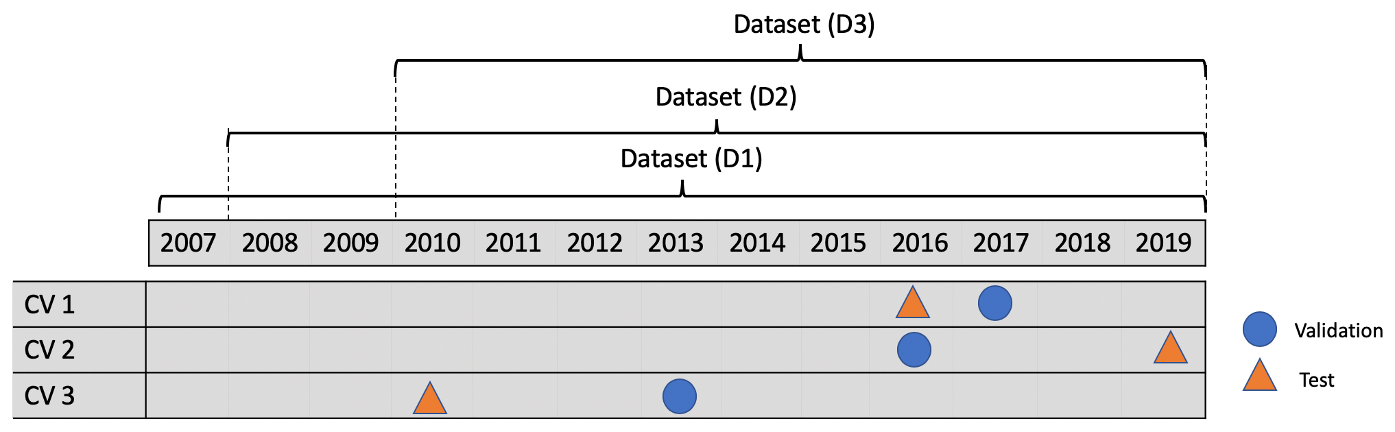
Figure 2 The three cross-validation datasets (CV 1, CV 2, and CV 3) consist of different training, validation, and testing samples from the 13 years ERA5 reanalysis data between 2007 and 2019. Each row represents one data partition. The three datasets (D1, D2, and D3) consist of samples from 2007 to 2019, from 2008 to 2019, and from 2010 to 2019, respectively.

We constructed three cross-validation experiments by selecting different non-overlapping data splits for training, validation, and testing (see Fig. 2). Thereby, we make use of 11 years of data for training, while 2 years are deployed for validation and testing with minimized auto-correlation following the discussion in Schultz et al. (2021). The cross-validation is applied to check the robustness of the trained models over a broad temperature range. By selecting 2010 (CV 3), 2016 (CV 1), and 2019 (CV 2) for the testing dataset, we ensure that our trained models are tested on years with relatively cool, on-average, and warm temperatures, respectively, within the chosen data period. During training, the validation loss (for tuning the model parameters) operates on data from 2013 (average), 2017 (warm), and 2016 (average).

To check how the model performance depends on the spatial domain size and on the provided information of the atmospheric state, we vary the spatial extent of the domain and the number of involved predictors. For the former, smaller target regions are tested; see Fig. 1. The latter is realized by removing TCC from the list of predictors in a first experiment and just inputting T_2 m in a second experiment. Additionally, we vary the number of training samples by cropping the training dataset and also check the sensitivity on the input sequence length, which was discussed to be relevant to encode the daytime in a data-driven way (see above). A comprehensive overview of the sensitivity experiments is provided in Table A1 of the Appendix.

Our approach shares some similarities with the study of Bihlo (2020) as we use the same dataset, a similar study region, and also focus on short-range predictions. However, besides the use of a different neural network architecture (SAVP in our case, cGAN in Bihlo, 2020), there are some distinct differences which make our application potentially more challenging. First, we approximately retain the spatial resolution of the ERA5 reanalysis data on a regular 0.3^∘ grid (compared to 0.5^∘). Besides, the temporal resolution is also considerably higher since we set the time step to 1 h compared to 3 h. By doing so, our models must learn to represent smaller features of the near-surface temperature field, and they must better capture the underlying diurnal cycle. By conditioning the model on its own predictions, errors are expected to accumulate quicker with an hourly time step.

3.3 Model architectures

In the following, we briefly introduce the three video prediction models probed in this study: a simple fully convolutional neural network (CNN), the convolutional LSTM (ConvLSTM) model, and the Stochastic Adversarial Video Prediction (SAVP) model. While a summary of the architectures is provided, more detailed descriptions can be obtained from the original studies by Rasp et al. (2020) on CNN, Xingjian et al. (2015) on ConvLSTM networks, and Lee et al. (2018) for SAVP. The current version of models and code are available and can be accessed from the project website (https://gitlab.jsc.fz-juelich.de/esde/machine-learning/ambs/-/tree/Gong2022_temperature_forecasts, last access: 1 July 2022).

3.3.1 A simple convolutional neural network (CNN)

Following up the study by Rasp et al. (2020), we deploy a simple CNN as one of the baseline models. The CNN consists of five layers, and each layer has 64 channels with a kernel size of 5. In contrast to the global forecasts with a spatial resolution of 5.625^∘ provided in Rasp et al. (2020), the target domain in our task is restricted to central Europe, and thus we did not apply periodic convolutions. The mean square error is optimized on the variables of interest (2 m temperature, temperature at 850 hPa, and total cloud cover) for 1 preceding hour. The model was trained for 20 epochs using the Adam optimizer with a learning rate of 0.0001 and batch size of 4. During forecasting, we use the previous model output as input for the next step, which allows us to obtain forecasts up to 12 h ahead (iterative forecasting).

Figure 3 Sketch of ConvLSTM architecture (based on arguments in Xingjian et al., 2015).

3.3.2 The convolutional LSTM (ConvLSTM) model

The ConvLSTM model employs convolutional operations which encode the spatial properties of the input data into a hidden state. Temporal coherence is preserved with the help of a gated LSTM, so that an encoded state from all input data is achieved at the end of the input sequence (the encoded atmospheric state over the previous 12 h in our case). The forecasting network then unfolds this state by conveying both the LSTM cells' states (cell and hidden state) and the predictions fed in sequentially to come up with a forecast over the next 12 h. Here, we employ a one-layer ConvLSTM network, i.e. one ConvLSTM layer followed by a 1 × 1 convolutional layer. A sketch of the model architecture is provided in Fig. 3. We used a batch size of 4 and epochs of 10. The model was trained using mean squared error as the loss function and Adam optimizer (Kingma and Ba, 2014) with a learning rate of l_r = 0.001.

3.3.3 The Stochastic Adversarial Video Prediction (SAVP) model

SAVP constitutes a combination of the GAN and the VAE architectures. The model is therefore best described by summarizing both components separately in the following subsections before we explain how these components are coupled together. The explanations are furthermore complemented by a sketch of the SAVP architecture provided in Fig. 4.

Variational autoencoder

The VAE part of SAVP consists of an encoder and a generator. The deep encoder E compresses the information from adjacent time steps into a low-dimensional latent vector Z_t−1 = $E({\stackrel{\mathrm{̃}}{\mathit{X}}}_t,{\stackrel{\mathrm{̃}}{\mathit{X}}}_{t-\mathrm{1}})$ where $\stackrel{\mathrm{̃}}{\mathit{X}}$ represents either ground data from the input sequence or previously predicted data (i.e. ${\stackrel{\mathrm{̃}}{\mathit{X}}}_t\in \mathit{\{}{X}_t,{\widehat{\mathit{X}}}_t\mathit{\}}$). Thus, E encodes the transition between the states at time steps t−1 and t into the latent representation Z_t−1, which is then fed to the deep generator G for reconstructing the state ${\widehat{\mathit{X}}}_t$. To control the latent space and to allow random sampling, the learned posterior distribution $q({\mathit{Z}}_{t-\mathrm{1}}\mid {\stackrel{\mathrm{̃}}{\mathit{X}}}_{t-\mathrm{1}:t})$ is kept close to a prior distribution p(Z_t−1). Thus, the loss component of the VAE part consists of the L₁ error constituting the reconstruction loss (first term in Eq. 1) and the Kullback–Leibler divergence $D_{\text{KL}}\left(q\right({\mathit{Z}}_{t-\mathrm{1}}\mid {\stackrel{\mathrm{̃}}{\mathit{X}}}_{t-\mathrm{1}:t})\parallel p({\mathit{Z}}_{t-\mathrm{1}}\left)\right)$, which acts to regularize the posterior distribution of the latent space onto the prior distribution (second term in Eq. 1). The latter constitutes a standard Gaussian distribution whose parameters are optimized with the help of the re-parametrization trick (Kingma and Welling, 2013).

Figure 4 Illustration of the SAVP architecture (based on discussion in Lee et al., 2018).

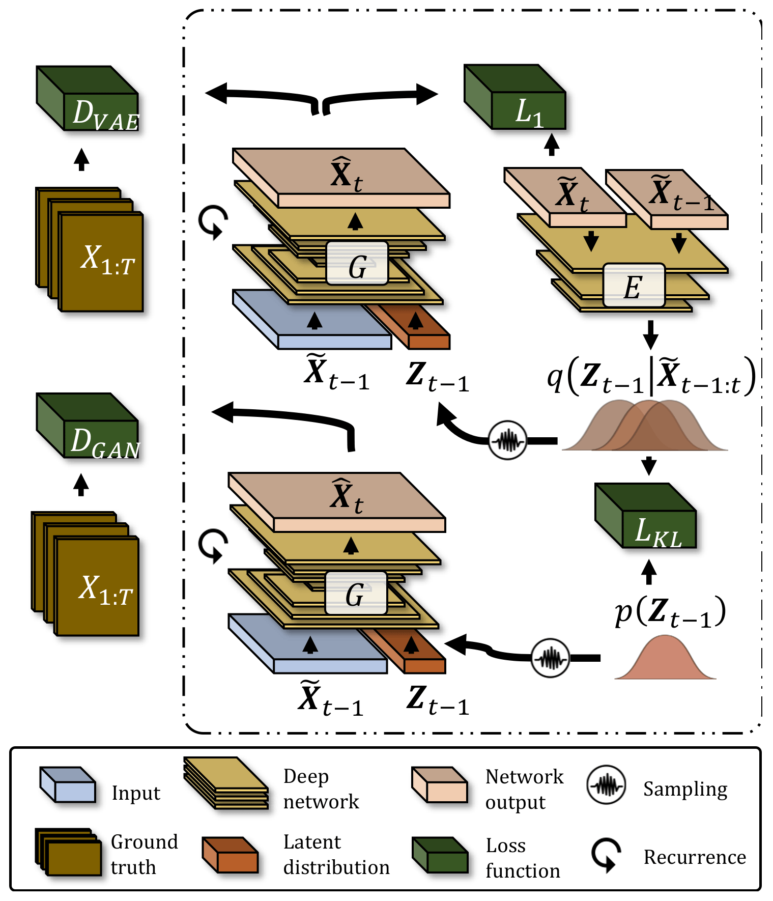
Generative adversarial network

The generator G in SAVP inputs the data from the previous time step ${\stackrel{\mathrm{̃}}{\mathit{X}}}_{t-\mathrm{1}}$, i.e. either ground truth or previously generated data, to reconstruct the data at time step t. Additionally, the generator is also conditioned on the latent space Z_t−1 via sampling. In GAN-based networks the generator G is thereby encouraged to learn the statistical properties of the underlying data. This is achieved by optimizing G to fool a deep discriminator D, which is itself optimized to distinguish between real data (i.e. the ground truth) and generated data. The loss function of the GAN ℒ_GAN in SAVP applies the binary cross-entropy loss for an adversarial minimax optimization. While the generator tries to minimize ℒ_GAN, the discriminator aims to maximize ℒ_GAN.

Combining VAE and GAN

For the SAVP architecture, one generator G is set up, which is shared between the VAE and GAN parts. However, two separate discriminators are used which are equivalent in terms of the architecture but differ in their trainable model parameters. The latter difference arises from the latent embedding that is fed to the shared generator G. For the discriminator related to the VAE part D^VAE, Z_t−1 is sampled from the posterior distribution $q({\mathit{Z}}_{t-\mathrm{1}}\mid {\stackrel{\mathrm{̃}}{\mathit{X}}}_{t-\mathrm{1}:t})$, whereas sampling from the prior distribution p(Z_t−1) is performed for the discriminator of the GAN part. Consequently, two GAN loss terms become part of SAVP's objective function (see Eq. 1), whose third and fourth terms are related to the GAN and VAE component, respectively. The total SAVP loss is calculated as

$$\begin{array}{}\text{(1)}& \begin{array}{rl}{G}^{\ast },E^{\ast }=& \text{arg}\underset{G,E}{min}\underset{D,D^{\text{VAE}}}{max}{\mathit{\lambda }}_{\mathrm{1}}{\mathcal{L}}_{\mathrm{1}}(G,E)+{\mathit{\lambda }}_{\text{KL}}{\mathcal{L}}_{\text{KL}}\left(E\right)\\ & +{\mathcal{L}}_{\text{GAN}}(G,D)+{\mathcal{L}}_{\text{GAN}}^{\text{VAE}}(G,E,D^{\text{VAE}}).\end{array}\end{array}$$

The discriminator architecture used by SAVP involves several convolutional layers that operate on the complete data sequence, followed by a fully connected layer. Three-dimensional convolutions are applied to handle the spatial and the temporal dimensions simultaneously. The shared generator G involves several ConvLSTM-layers with internal skip connections. These are followed by two convolutional layers to predict the state at the next time step. A separate composite mask is used to identify features from the data that are displaced between the time steps (e.g. a cold front in our meteorological application). In total, the number of trainable model parameters sums up to about 14 M. More details on the architecture are provided in Lee et al. (2018).

The default hyperparameters and training schedule in this study have been modified from the original description in Lee et al. (2018). During training, the initial learning rate used with the Adam optimizer is set to l_r = 2 × 10⁻⁴. The training applies linear learning rate decay to l_r = 2 × 10⁻⁸ between the iteration steps 3000 to 9000. With a batch size of 32, this roughly corresponds to the start of the second epoch and the end of the third epoch, respectively. Overall, the model is optimized on four epochs. For the scaling factors of the different loss components, we choose λ₁ = 10 000 and λ_KL = 0.01. Note that variations in λ₁ receive special attention in our sensitivity analysis below. The scaling factor for the distance in features space is set up to 0.001. Furthermore, the reconstruction loss only accounts for T_2 m, which differs from common computer vision applications where all channels enter this loss term.

3.4 Evaluation metrics

For evaluating the video frame prediction models introduced above, we make use of metrics that are commonly applied in the meteorological domain as suggested by Rasp and Thuerey (2021). In particular, we calculate the mean square error (MSE) and the anomaly correlation coefficient (ACC) for the predicted T_2 m fields (cf. Appendix Eqs. B1 and B2). While the MSE measures the mean squared distance between the predicted and the analysed (ground truth) temperature field, the ACC quantifies the agreement in the spatial patterns of departures from the climatological mean. Thus, the ACC is a positively oriented score with a perfect value of 1, whereas the MSE is negatively oriented with a perfect value of 0. In this study, we make use of the uncentred ACC (see Eq. B2) and calculate the climatological mean based on 30 years of data (1991–2020) provided by the ERA5 dataset. The climatological mean is computed for each month of the year and each hour of the day separately. This ensures that the seasonal and diurnal cycle of the near-surface temperature is incorporated.

In addition to the meteorological evaluation metrics, we also choose the structural similarity index (SSIM) which is commonly applied in video prediction to access the perceptual similarity between images (Wang et al., 2004). Transferring to this application, the SSIM quantifies and compares the mean as well as the spatial variability in the predicted 2 m temperature field against the ground truth and also accounts for covariances (cf. Eq. B7). Although being an evaluation metric from computer vision, it is considered to provide useful information on the forecast quality. Like the ACC, the SSIM is a positively oriented score with a perfect value of 1.

To evaluate the truthfulness of the predicted spatial variability, we also compute the domain-averaged amplitude of the horizontal T_2 m gradient. Similar to Sha et al. (2020), we then calculate the ratio r_G of the gradient amplitude from the predictions and the respective ground truth (see Eq. B10). For $r_{\mathrm{G}}(X,\widehat{X})=\mathrm{1}$, the predictions share the same local spatial variability as the ERA5 reanalysis data, while $r_{\mathrm{G}}(X,\widehat{X})<\mathrm{1}$ ($r_{\mathrm{G}}(X,\widehat{X})>\mathrm{1}$) indicates that the local spatial variability is underestimated (overestimated) in the predictions. This metric is similar to the sharpness measure introduced in Mathieu et al. (2015) but takes the Earth's curvature into account and does not scale to the maximal gradient amplitude.

While further details on all evaluation metrics are provided in Appendix C, we verify our models against the persistence forecast in terms of skill scores for convenience. This allows a direct comparison with a reference model which attains a value of S_ref for the respective score S. As a reference model, we use a simple persistence model which is based on the assumption that today's weather is the same as yesterday's; i.e. the temperature field from the last day is simply copied. Together with the perfect score value S_per, the skill score SS_S reads

$$\begin{array}{}\text{(2)}& {\displaystyle }{\text{SS}}_{\mathrm{S}}={\displaystyle \frac{S_{\mathrm{m}}-S_{\text{ref}}}{S_{\text{per}}-S_{\text{ref}}}},\end{array}$$

where S_m denotes the score value of the considered model forecast.

4 Results

In the following, we evaluate the predictive skill of the SAVP and ConvLSTM models for 2 m temperature predictions up to a lead time of 12 h. For the presented model results, our default hyperparameters of both models have been tuned to yield the best results in terms of the MSE. However, we also provide an ablation study on the L1 loss component in the SAVP model and also probe the sensitivity with respect to input variables, regions, and the size of the training dataset.

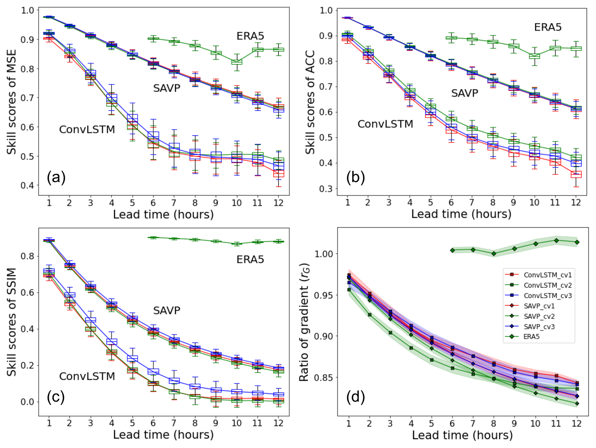
Figure 5 Averaged skill scores of (a) MSE, (b) ACC, and (c) SSIM across lead time (x axis) for the SAVP and the ConvLSTM models as well as ERA5 short-range forecasts. Both video prediction models are trained with the three cross-validation datasets (with CV 1–3 in D1) displayed in Fig. 2. The testing period of the ERA5 short-range forecasts covers the year 2019, which corresponds to CV 2. The persistence serves as the reference forecast. Sampling uncertainty estimated via block bootstrapping is illustrated by box-and-whisker plot showing the inter-quartile and inter-decile ranges of the skill score values. Panel (d) shows the ratio of the spatially averaged 2 m temperature gradient for the same video prediction models and ERA5 short-range forecasts. The persistence forecasts (not shown) attain a constant value of r_G=1 since local spatial variability is retained.

4.1 Model performance analysis

The skill scores in terms of the MSE (Fig. 5a), the ACC (Fig. 5b), and the SSIM (Fig. 5c) are displayed in Fig. 5. The uncertainty estimates depicted by the boxes and whiskers are derived through block bootstrapping with a block length of 7 d (Efron and Tibshirani, 1994). It is seen that all video prediction models outperform the persistence forecast significantly over the complete prediction period. The constant MSE of the persistence forecast (MSE(Persistence)≃ 7 K²) is reduced by about 50 % for ConvLSTM and by about 70 % for the SAVP model over the prediction period. Likewise, both models also clearly provide better forecasts of local temperature anomalies from the climatological mean (ACC(Persistence)≃ 0.67) as seen from Fig. 5. Only with respect to the SSIM (SSIM(Persistence)≃ 0.66) does the ConvLSTM model lose its forecast skill after a lead time of 7 h (Fig. 5c). In many aspects, the SAVP model also clearly performs better than the ConvLSTM model: the MSE skill score degrades linearly and at a much smaller rate, especially over the first 6 h. After 12 h, the MSE of SAVP tracks at about 2.3 K², while the ConvLSTM model shows up with an MSE slightly above 3.6 K² (absolute score values are displayed in Fig. C2 of the Appendix). Similarly, the ACC and the SSIM remain closer to 1 for the SAVP model (ACC(SAVP)≃ 0.87 > ACC(ConvLSTM)≃ 0.80 and SSIM(SAVP)≃ 0.73 > SSIM(ConvLSTM)≃ 0.67). Thus, as expected, the more complex SAVP model can learn a better representation of the atmospheric state and therefore produces a better prediction of the diurnal cycle of the 2 m temperature compared to ConvLSTM.

However, even though the global variability as expressed by the SSIM is better captured with SAVP, the local spatial variability is scarcely better than in the ConvLSTM model. In terms of the horizontal gradient ratio, the forecasts of both models degrade continuously with increasing lead time, yielding a noticeably underestimation by the end of the forecast period (see Fig. 5d). Thus, the predicted 2 m temperature fields of both video prediction models become too smooth indicating that small-scale variations due to the underlying topography (mountain ranges) and surface type (costal regions) get blurred.

Furthermore, we compare the performance of the video prediction models against the short-range forecasts provided with the ERA5 dataset. These forecasts are initiated at 06:00 and 18:00 UTC with a maximum lead time of 18 h. Since the changes in the assimilation window at 09:00 and 21:00 UTC introduce a systematic shift with respect to the reference reanalysis data, the presented scores are limited to lead times between forecast hour 6 and 12. It is seen that there is still a significant gap between the data-driven approaches and the contemporary NWP models which are driven by the fundamental laws of physics. The skill scores of the ERA5 short-range forecasts in terms of the proposed evaluation metrics are higher than the video prediction model and closer to the best score of 1.

In addition, we evaluate the performance of the CNN with iterative forecasting from Rasp et al. (2020). The results reveal that the iterative CNN forecasts can only beat the persistence forecasts up to 4 h lead time. After that, the model error accumulates quickly and even becomes highly unstable after forecast hour 10, when the MSE starts to exceed 100 K² (not shown). Thus, it is evident that the CNN performs considerably worse than the simple ConvLSTM model which shows that pure CNN models fail to capture the temporal dependency of the data and to obtain skilful forecasts for longer lead times. Recurrent layers are required to transit temporal information, which in turn is highly relevant to stabilize the model's long-term forecasting performance.

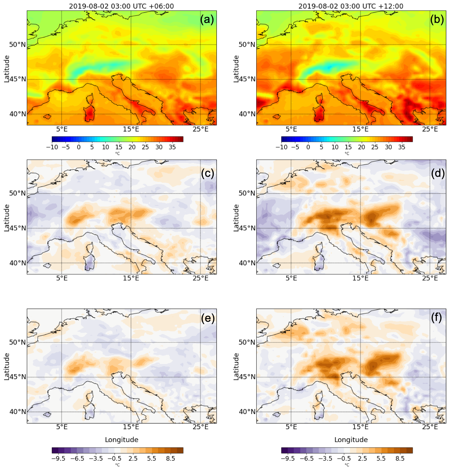
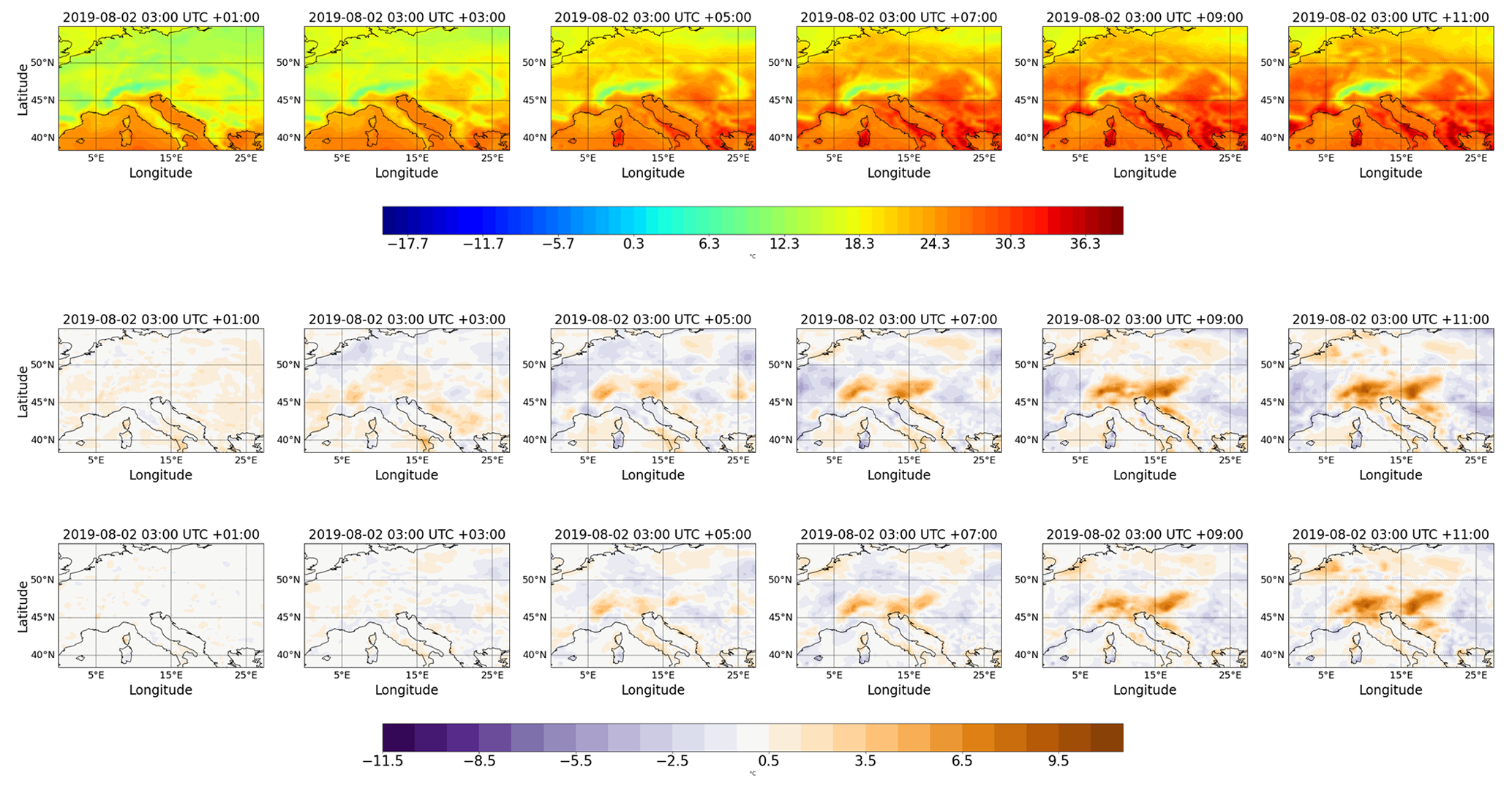
Figure 6 Example forecast for the 2 m temperature with a lead time of 6 (panels a, c, and e) and 12 h (panels b, d, and f). (a, b) The ground truth from the ERA5 reanalysis dataset. (c, f) The difference between the forecasts generated by the ConvLSTM (c, d) and SAVP (e, f), where positive (negative) values represent a warm (cold) bias in the forecasts. The initial time for both model forecasts is 2 August 2019, 03:00 UTC. Further time steps of the 12 h predictions are provided in Appendix C6.

To illustrate concretely our statistical findings, we show a representative case study of ConvLSTM and SAVP forecasts starting on 2 August 2019, 03:00 UTC. The first row in Fig. 6 shows the 2 m temperature field from the ERA5 reanalysis (ground truth) for a lead time of 6 and 12 h. The differences in the respective ConvLSTM and SAVP model forecasts are presented in the second and third row, respectively, with positive values corresponding to a warm bias.

Apart from growing differences to the ground truth with increasing lead time where SAVP exhibits smaller errors on average, both models forecast strong warming over continental areas. Thus, aspects of the diurnal cycle are captured by the video prediction models. However, it is also noted that the forecast accuracy especially deteriorates around the Alpine region, indicating that both models have problems in predicting the temperature evolution in this area. Besides, differences appear to be bounded by the coastal line with dipole structures visible in the Mediterranean region. This indicates that strong spatial gradients in 2 m temperature tend to be blurred in accordance with the findings in Fig. 5d.

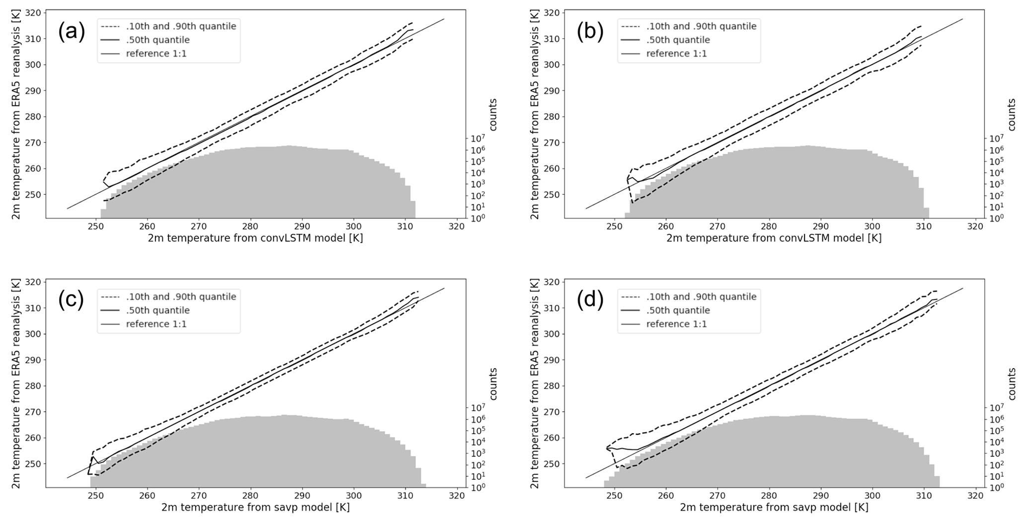
Figure 7 Conditional quantile plots in terms of the calibration-refinement factorization for 2 m temperature forecasts with a lead time of 6 h (a, c) and 12 h (b, d). Panels (a, b) show the factorization of ConvLSTM forecasts, while (c, d) correspond to the SAVP model. The solid straight line denotes the 1:1 reference line of a hypothetical perfect model. The dashed lines represent the 10th and 90th quantiles, and the bold solid line represent the median of the ground truth data conditioned on the forecasts, respectively. The marginal distribution of the model forecasts is presented as log histogram (right axis, light grey bars).

Further insight into the statistical properties of the forecast with respect to the ERA5 reanalysis (the ground truth) can be obtained from conditional quantile plots. These plots visualize important aspects of the joint distribution of forecast and reference data for continuous variables by factorizing it into a conditional and a marginal distribution (Murphy and Winkler, 1987; Wilks, 2011). Figure 7 shows the full joint distribution in terms of the calibration-refinement factorization for lead times of 6 and 12 h. The median as well as the inter-decile ranges of the ground truth conditioned on the forecasts are displayed by the solid and dashed lines, respectively. The histogram at log scale illustrates the marginal distribution of the respective model forecast.

The central parts of the temperature range are well calibrated in both models, but the ConvLSTM model shows a broader inter-decile range in accordance with the larger MSE. Larger deviations from the 1:1 line are obtained near the tails of the conditional distributions in all four panels. Thus, both models have problems issuing calibrated forecasts when the 2 m temperature is very high (around 310 K) or very low (around 250 K). It is noteworthy that the marginal distribution of the ConvLSTM model results becomes narrower for longer lead times since no temperatures below 252 K (10 out of 8471 samples) are predicted. By contrast, the SAVP model predicts up to 4 K colder temperatures even for forecast hour 12, although the forecasts are not well calibrated at the lower tail of the conditional distribution. A similar result, but with a smaller amplitude, can also be deduced at the upper tail of the conditional distributions. Thus, the SAVP forecasts exhibit a slightly higher degree of refinement, also termed sharpness in statistics (Wilks, 2011), compared to ConvLSTM.

4.2 Trade-off between sharpness and accuracy

The term “sharpness” has different meanings in the computer vision and meteorological domains. Sharpness in meteorology characterizes the unconditional distribution of the forecasts. A sharp forecast means that the forecasts are frequently enough distinctly different from the climatological value of the predictand. By contrast, sharpness describes the image contrast at the object edges in the computer vision domain. In the following, we discuss sharpness in this latter sense and analyse the local spatial variability of the 2 m temperature fields in terms of the gradient ratio.

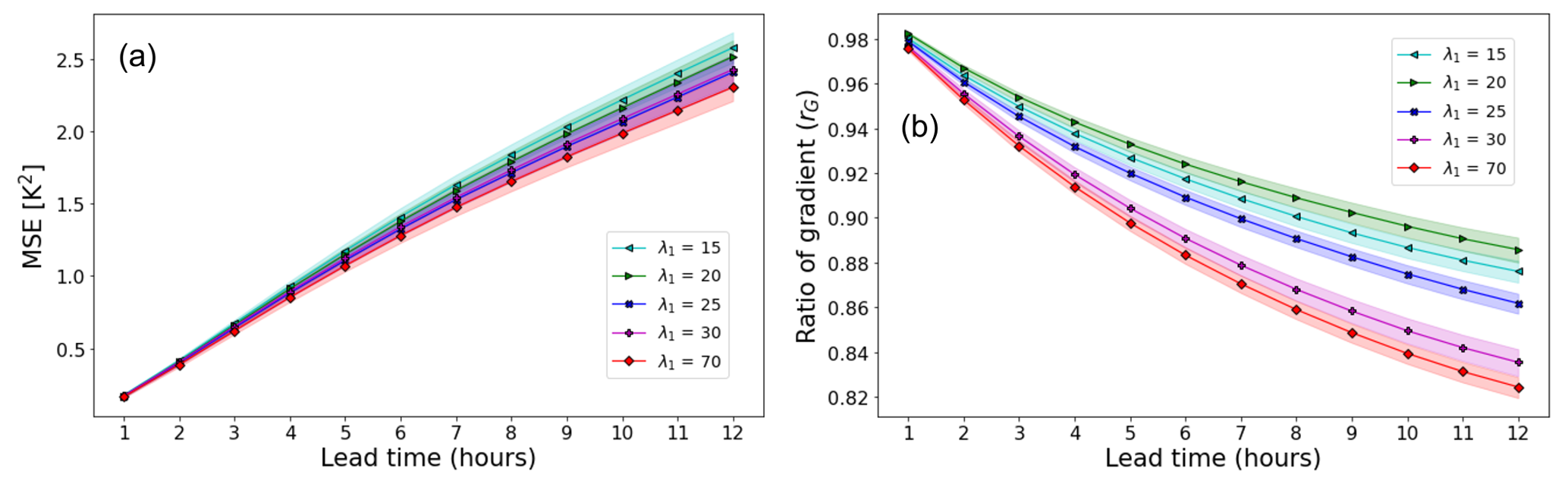
Figure 8 Performance of the SAVP model in terms of (a) MSE and (b) the gradient ratio r_G with variations in the scaling factor for the L1 loss λ₁. Note that the results for λ₁=70 only differ marginally from using λ₁ = =10 000.

Sensitivity tests were performed by varying the L1 loss scaling factor λ₁ in Eq. (1). While the results are rather insensitive for λ₁ > 100 (not shown), we notice a stronger dependency of the model performance for smaller values of λ₁. The image sharpness is improved particularly for longer predictions for smaller scaling factors of the L1 loss, while the MSE is slightly increased (see Fig. 8). This implies that the GAN component in SAVP is largely responsible for maintaining the feature contours. By reducing the strong weight of reconstruction loss, the SAVP model is encouraged to produce temperature fields with a higher local variability, although the errors at grid-point level become larger then.

Note that such a trade-off between sharpness in terms of the gradient ratio and accuracy in terms of MSE is observed in weather forecast applications as in other computer vision applications (Lee et al., 2018).

This sensitivity study also explains why the SAVP in its original configuration does not outperform the ConvLSTM model in terms of the gradient ratio (Fig. 5). Due to the very large value of the L1 scaling factor (λ₁ = 10 000), the model is encouraged to optimize for the pixel-wise loss over other losses (e.g. the adversarial loss). Thus, the outperformance in terms of MSE, ACC, and SSIM can be attributed to the more sophisticated generator architecture in SAVP alone rather than the adversarial optimization.

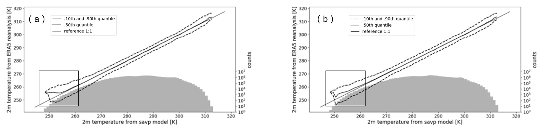
Figure 9 Conditional quantile plots in terms of the calibration-refinement factorization for 2 m temperature forecasts with a lead time of 12 h of the SAVP model with (a) λ₁ = 10 000 and (b) λ₁ = 15.

In order to gain additional insight into the performance of the GAN component in SAVP on the tails of the 2 m temperature distribution, two conditional quantile plots generated with λ₁ = 10 000 and λ₁ = 15 are provided in Fig. 9. While there are no significant differences for large parts of the conditional distribution, we observe that the median gets closer to the 1:1 reference line at the lower tail of the PDF for λ₁ = 15. Thus, lowering λ₁ also yields better-calibrated model forecasts for very cold temperatures. Note that the lowest temperatures occur in the Alpine region for our target region where grid points are located more than 2000 $\mathrm{m}\mathrm{a}.\mathrm{s}.\mathrm{l}.$ (see Fig. 1). Since the surface elevation varies quite strongly over the mountainous region, the preservation of large local temperature gradients due to the underlying topography is a necessary prerequisite for well-calibrated forecasts in this region.

4.3 Sensitivity analysis

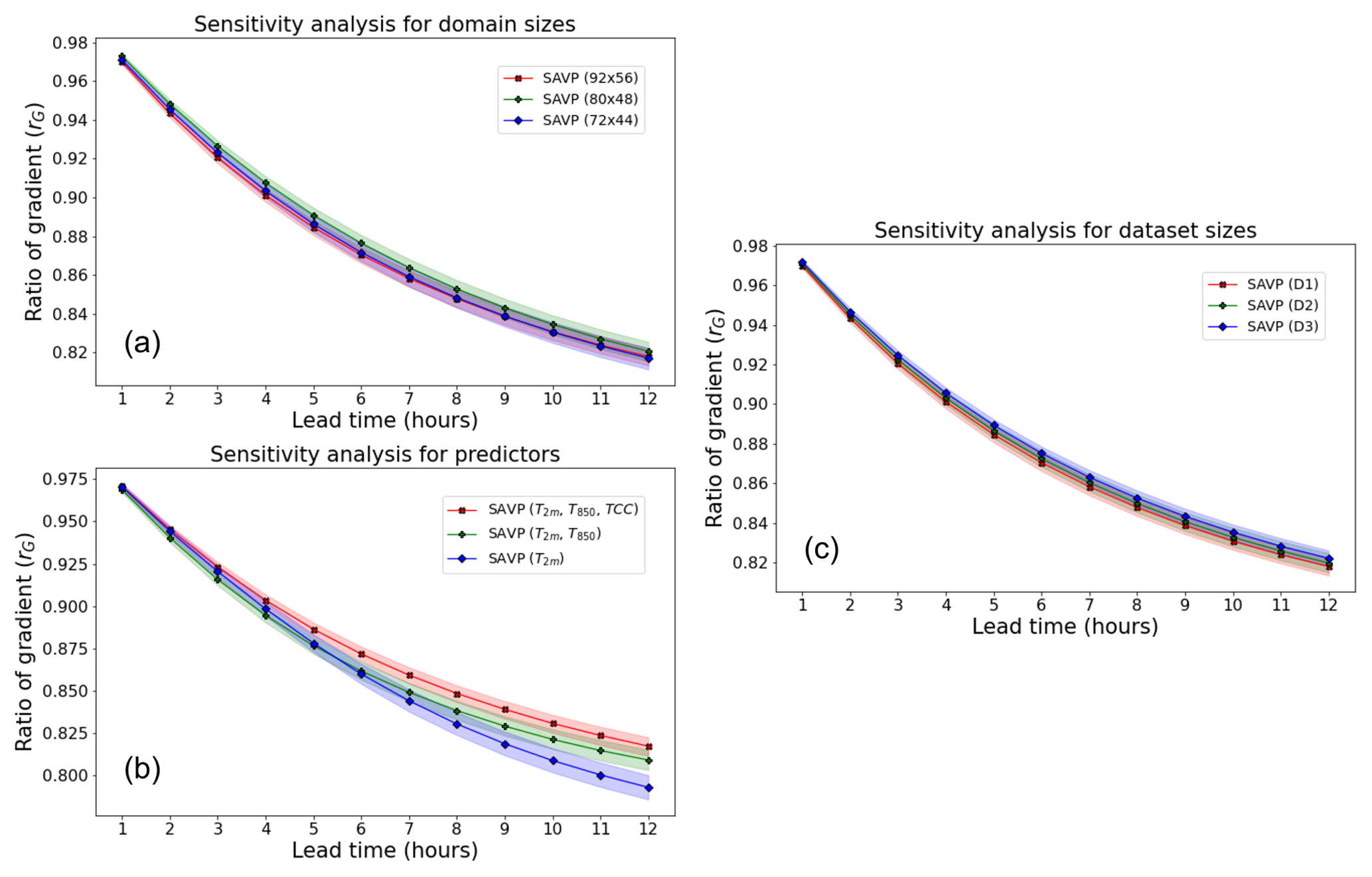
In the following, we describe further sensitivity tests on the domain size, the selected predictor variables, and the amount of training data of the SAVP model (Experiments 2, 3, and 4; cf. Table A2 in the Appendix). The analysis thereby focuses on evaluating the model performance in terms of the MSE. However, the results of the other evaluation metrics are also briefly presented and the corresponding plots are attached to Appendix C.

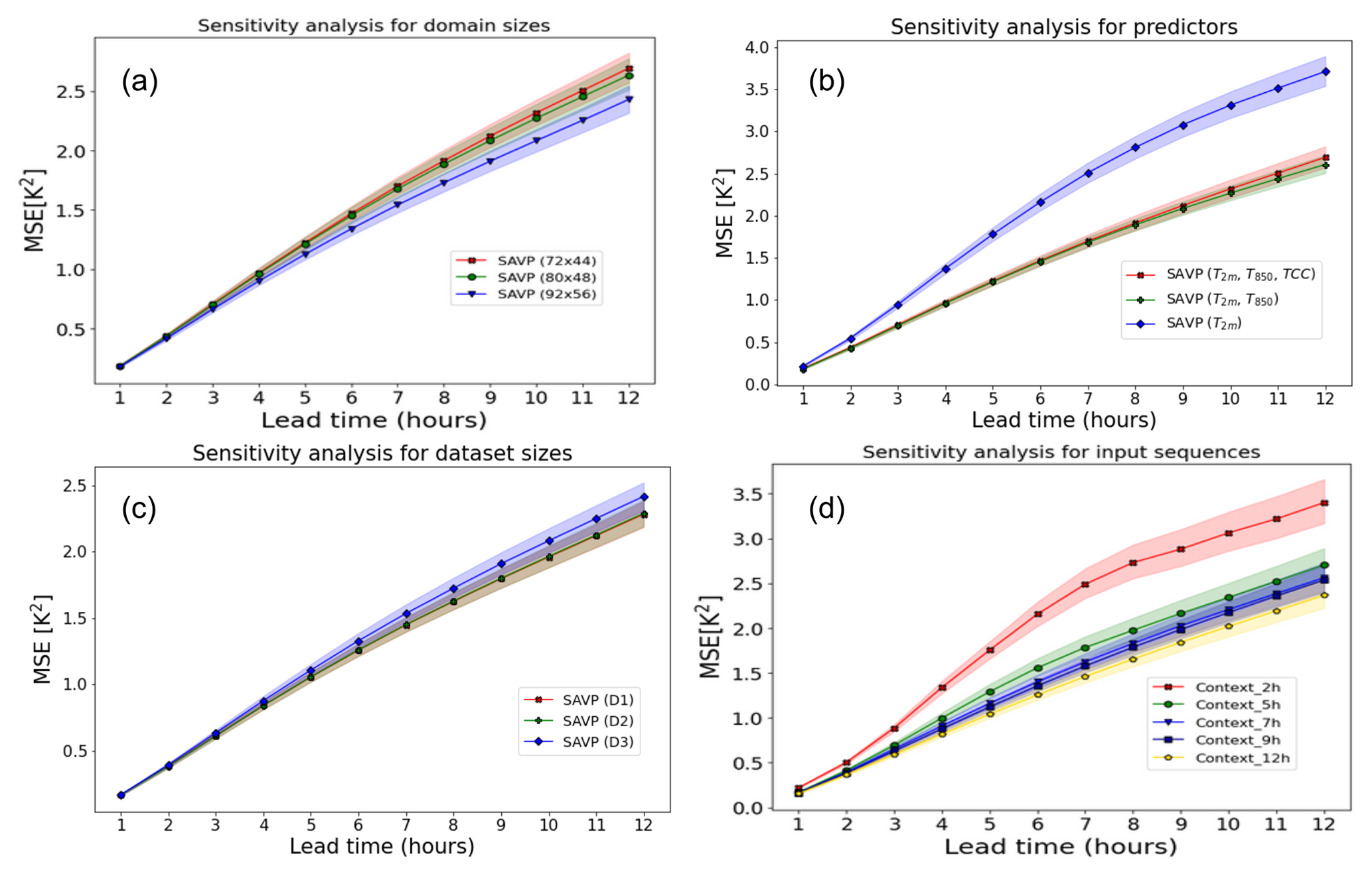
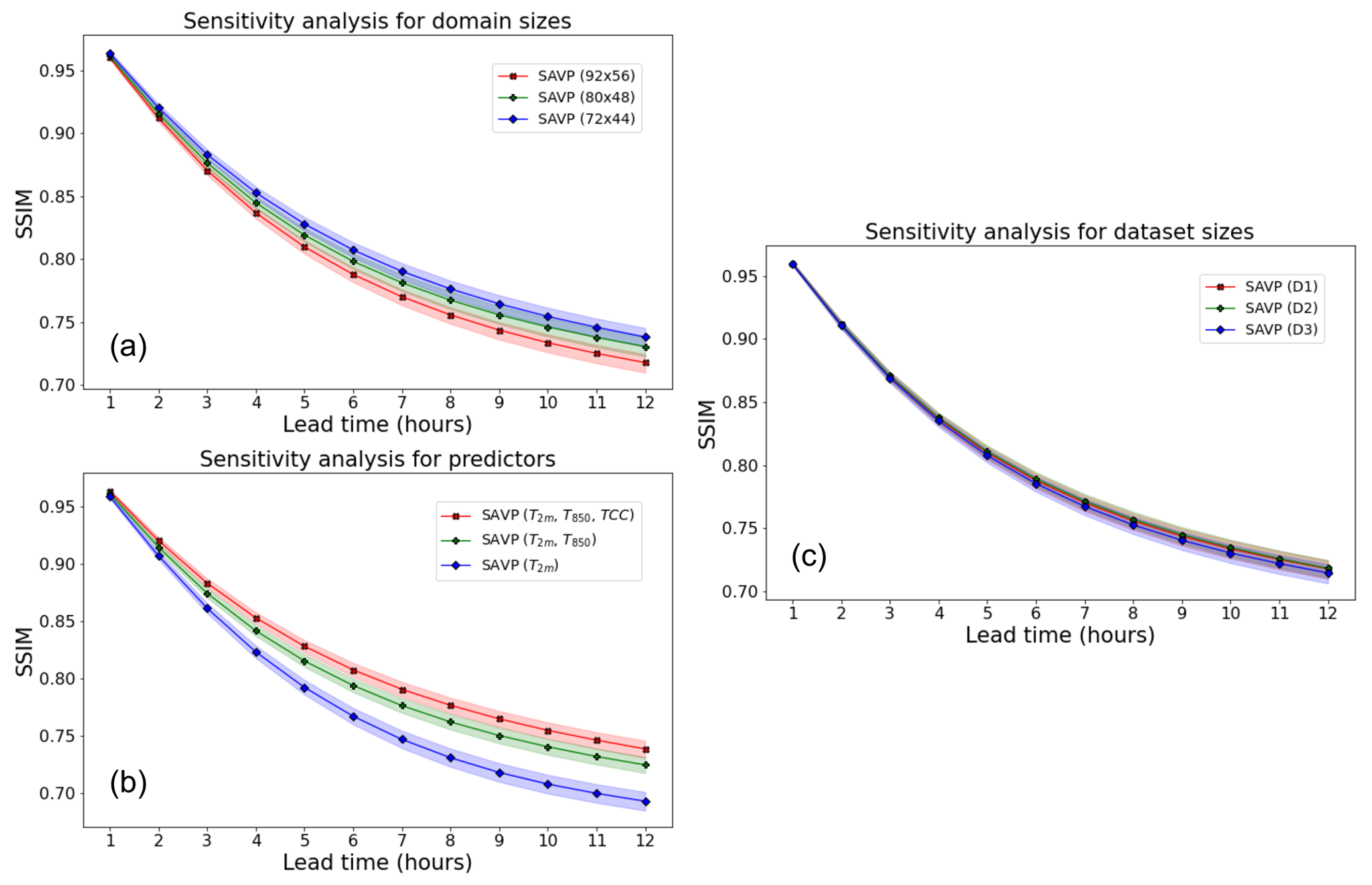
Figure 10 Averaged MSE of 2 m temperature forecasts with the SAVP model for different sensitivity experiments using (a) different domain sizes (red – 92 × 56; green – 80 × 48; blue – 72 × 44), (b) different predictors (red – T_2 m, T_850 hPa, and TCC; green – T_2 m, T_850 hPa; blue – T_2 m), (c) different sizes of the training dataset (red – 11 years; green – 10 years; blue – 8 years), and (d) different input sequence lengths. The sampling uncertainty estimated via block bootstrapping is denoted by colour shading.

The models in Experiment 2 are trained on data from all 11 years, but the domain size is reduced from 92 × 56 to 80 × 48 and 72 × 44. Note that the evaluation for this experiment is conducted on the inner 72 × 44 domain to allow for direct comparison. It is seen that the performance in terms of the MSE slightly deteriorates when the target domain becomes smaller (Fig. 10a). Interestingly, the reduction in MSE is most pronounced when enlarging the target domain from 80 × 48 to 92 × 56 (reduction in MSE by about 0.2 K²). Similar results are obtained in terms of the ACC. However, in terms of the SSIM and the gradient ratio r_G only minor changes due to variations in the domain size are observed.

In Experiment 3, the set of predictor variables is reduced gradually from three (T_2 m, T_850 hPa, TCC) to two (T_2 m, T_850 hPa) and further to one (T_2 m). Note that this experiment is conducted on the smaller target domain with 80 × 48 grid points, on which the average MSE tracks about 0.2 K² higher than on the largest domain with 92 × 56 grid points. While the MSE is fairly insensitive with respect to the inclusion of the TCC, a significant increase is observed when T_850 hPa is dropped from the list of predictors. For the former case, the MSE is just increased by about 0.1 K², whereas the latter results in an MSE of 3.7 K² after a lead time of 12 h. Thus, the temperature of the air mass is more relevant than the total cloud cover for predicting the diurnal cycle of 2 m temperature in our study. In terms of the other evaluation metrics (ACC, SSIM, and r_G), similar results are obtained.

To evaluate the impact of the number of training samples on the forecasting performance, the size of the training dataset is reduced from 11 years in D1 to 10 years in D2 and 8 years in D3 (see Fig. 2). For the sake of a fair comparison, we fixed the validation dataset to 2016 and the testing dataset to 2019, respectively. Removing a single year from the training dataset does not affect the model performance in terms of the MSE (Fig. 10c). When 3 years of data are dropped from the training dataset, we notice a slight deterioration (MSE increases to about 2.45 K² from 2.3 K²). In terms of the ACC, the SSIM, and r_G, the model performance is also rather insensitive to the variations in the size of the dataset probed in this study.

To identify whether the models could infer the daytime without providing explicit daytime information, we design Experiment 5, where the length of the input sequence is varied. We notice that providing one half of the diurnal cycle (12 preceding hours) as input yields the best model performance in terms of the MSE (see Fig. 10d). Reducing the length of the input sequence from 12 h to 5 h results into a successive degradation of model performance. Although the increase in MSE is only about 0.3–0.4 K² for a lead time of 12 h, its impact is stronger than removing 3 years of training data or than removing TCC from the list of predictors.

A further significant degradation of model skill takes place when the input sequence is restricted to the 2 preceding hours. The MSE then becomes similar to the experiment where the 2 m temperature itself was input as the predictor. In terms of the ACC and the SSIM, the sensitivity of the results is similar; however for the gradient ratio, we do not observe a significant impact of input sequence length.

5 Discussion

The results presented in the previous section demonstrate that video frame prediction models from computer vision attain some predictive skill in forecasting the diurnal cycle of 2 m temperature. We showed that the SAVP model performs significantly better than a simple ConvLSTM model in terms of several evaluation metrics (MSE, ACC, and SSIM). This confirms our expectation that more advanced DL can better extract spatio-temporal features from the input sequence to predict the future state, which in turn is beneficial for meteorological applications, even though these models are originally developed for applications in computer vision.

However, the local spatial variability as measured in terms of the gradient ratio is not necessarily improved in our experiments with the SAVP model. Experiments with varied scaling factors of the L1 loss component λ₁ reveal that the strong weight on the pixel-wise reconstruction loss in our basic hyperparameter setting (cf. Sect. 3.3.3) is responsible for this behaviour. With λ₁ = 10 000, the adversarial part of the SAVP architecture is effectively neglected. Thus, the improvement seen in the evaluation metrics can be attributed to a more advanced generator which incorporates ConvLSTM cells, several convolutional layers along with skip connections and conditioning information on latent code. Reducing λ₁, the accuracy of the model in terms of the MSE slightly decreases, but the local spatial variability becomes much more similar to the ground truth data. In other words, the adversarial training with the GAN components encourages the model to preserve local features in the 2 m temperature field which can be attributed to spatial variability due to varying characteristics of the Earth's surface. Note that the latter characteristics (e.g. land–sea contrast and surface elevation) have not been explicitly fed to the models, so that their impact needed to be learnt in a data-driven way. Additionally, the forecasts tend to be better calibrated for very cold conditions. Since very cold conditions constitute the tail of the marginal distribution of 2 m temperature, it is hypothesized that the GAN component in SAVP may help to forecast extreme temperature events.

Further sensitivity experiments reveal that the prediction of the diurnal cycle of 2 m temperature can significantly benefit from incorporating additional predictors. In particular, the temperature at 850 hPa provides additional information on the air mass characteristics, which in turn yield a strong reduction in the MSE by at least 30 %. However, adding the total cloud cover surprisingly barely contributed although clouds drive the energy fluxes at the surface, which in turn drive the diurnal cycle of near-surface temperature and the planetary boundary layer in general (e.g. von Engeln and Teixeira, 2013; Chepfer et al., 2019). One reason for this result might be that the model has problems in predicting the future cloud cover since the underlying microphysical processes are highly complex (see, e.g., Khain et al., 2015) and that we only optimize the model on the 2 m temperature. While this turned out to be beneficial in our study (not shown), meaningful feature abstraction from quickly varying predictors becomes challenging.

Furthermore, the model performance is slightly improved upon enlarging the target domain. On the one hand, this might be attributed to an improved feature abstraction of the large-scale atmospheric conditions (e.g. the advection of air masses). On the other hand, the synoptic-scale features have limited relevance at sub-daily timescales since the time and spatial scales of atmospheric processes are correlated (see, e.g. Orlanski, 1975). Besides, the largest domain of 92 × 56 grid points includes the largest fraction of marine pixels. Since the 2 m temperature exhibits much smaller diurnal variations over the sea surface (Ginzburg et al., 2007), the prediction becomes simpler for these regions, which in turn translate to smaller prediction errors (see also Fig. 6).

In addition, the MSE of the SAVP model trained with 11 years of data is slightly decreased, but compared to the additional amount of data included (37.5 % compared to the 8-year dataset), the effect is judged to be minor. We argue that the dataset should probably not include fewer data than probed here, but, contrarily, including more data from the ERA5 reanalysis database is not expected to provide substantial benefits. It could even be that stronger climate change signals may outweigh the added value of including more data to the training dataset.

It is worth mentioning that using one half of the diurnal cycle of 2 m temperature as input is beneficial to model's forecasting capability. Limiting the input sequence to only 2 h yields a strong increase in the MSE by about 1.5 K², which is equivalent to removing all informative predictors besides the 2 m temperature itself. Since the performance already deteriorates for smaller changes to the input sequence, we conclude that the model can infer the daytime from the input sequence in a data-driven way provided that it covers at least one half of the day.

Our study shares some similarities with the study of Bihlo (2020), which also presents short-range forecasts of the 2 m temperature over Europe with a GAN-based model. While his predictions attain a fairly low RMSE of about 0.53 K for 12 h forecasts, which is considerably smaller than the model performance with our SAVP model (RMSE(SAVP) = $\sqrt{\text{MSE}\left(\text{SAVP}\right)}\simeq$ 1.5 K), direct comparison is limited due to relevant changes in the target of the forecast product. First, the spatial resolution of the target product is higher with 0.3^∘ compared to 0.5^∘, and, thus, local spatial variability must be captured more precisely in our case study. Second, we choose an hourly forecast product to focus explicitly on the predictability on the diurnal cycle. Thus, 12 consecutive forecasts are required to generate a 12 h forecast with our SAVP, which is considerably more than four time steps in Bihlo (2020). Thus, the increased temporal resolution of our forecasts come at the price of a stronger error accumulation, since the forecasts are conditioned on the previous hour.

Furthermore, we notice that the gap between data-driven neural networks for meteorological forecasts and contemporary NWP models is still considerable. While an RMSE of 1.5 K for a 12 h forecast is attained with our SAVP model, contemporary global NWP models show up with an RMSE of about 0.4 K.¹ Meanwhile, they also provide a higher spatial solution of around 0.1^∘ ≃ 10 km. However, in light of the long development history of NWP models for several decades (Bauer et al., 2015), the results with data-driven neural networks are already encouraging. Thus, further research, as presented in the following section, may further close the gap between deep neural networks and classical NWP models.

6 Conclusion

In this study, we have explored the application of video prediction models, originally developed for computer vision applications, to forecast the sub-daily temperature evolution over Europe. While the results show that more sophisticated model architectures such as the SAVP model and the inclusion of informative predictors such as the 850 hPa temperature can significantly improve the model performance, we also shed further light on the orchestration of different loss components in the composite SAVP architecture. Tuning the model on the L1 loss optimizes for the MSE but also leads to a strongly underestimated local spatial variability. Conversely, choosing a smaller weight on the L1 loss leads to a slight increase in MSE, but the spatial variability is better preserved due to a relatively stronger contribution of the GAN component in SAVP.

The findings in our study and the persisting large gap to NWP models motivate future work which aims to improve the performance of the underlying deep neural networks. First, one may consider testing further state-of-the-art video prediction models from computer vision which continue to develop at a quick pace. Further advanced GAN-based models (e.g. Brock et al., 2019; Clark et al., 2019; Qi et al., 2020) or the recent success in vision transformers (e.g. Caron et al., 2021; Yan et al., 2021) are appealing candidates which may help to reduce the above-mentioned gap. Apart from improving the model architecture, our results also suggest that deep neural networks can benefit greatly from adding further predictors beside the target variable to further improve the forecast skill. In our case, the 850 hPa temperature proved to be beneficial for the model performance, and it is likely that other dynamic predictors such as surface fluxes or near-surface wind can contribute to the model performance as well. Also static fields such as surface elevation and the land–sea mask should be considered (Sha et al., 2020; Lezama Valdes et al., 2021). Thus, a more systematic predictor selection is an appealing candidate to further improve the forecast skill.

Another way would be to exploit explicitly physical knowledge. This could be realized during preprocessing via feature engineering or during training by formulating physical constraints (de Bézenac et al., 2019; Karniadakis et al., 2021). In some cases, even simple physical constraints can be beneficial and can furthermore increase the realism when predictions beyond the training data space need to be issued (Karpatne et al., 2017). Additionally, enlarging the forecast domain is considered to be helpful, especially when the lead time is extended. For medium-range forecasts, even a processing of the global atmospheric state helps, but it is mentioned that this would result into enormous memory requirements on the operating GPU used for training, at least when a highly resolved forecast product is demanded (cf. Dueben and Bauer, 2018).

Due to the multi-scale, non-linear interactions in atmospheric processes, the uncertainty in weather prediction tends to be large (see, e.g., Lorenz, 1969), and quantifying this uncertainty is considered to be crucial in meteorology (Vannitsem et al., 2021). The demand for a probabilistic framework further increases when other meteorological quantities such as precipitation are targeted, which involve a high degree of inherent uncertainty due to the chaotic dynamics of small-scale processes. The SAVP model can also be used for probabilistic forecasting by adding white noise to the generator or via sampling from the latent space of the VAE component. The VAE component encodes the input into the latent representation that returns a distribution instead of a single point. The decoder synthesizes the frames by sampling random latent code from this distribution. This approach proved to be effective in generating more diverse samples on machine learning benchmark datasets in computer vision (Lee et al., 2018), but it has to be checked if this also applies to meteorological forecasting tasks.

Precipitation is a typical example for such a meteorological quantity since it is subject to complex interacting microphysical and dynamical processes on small spatio-temporal scales (Sun et al., 2014). While precipitation nowcasting is already gaining momentum in the meteorological community (Prudden et al., 2020), video prediction models may also be helpful to extend the forecast range beyond a few hours. This is motivated by the fact that even contemporary NWP models still have problems in predicting precipitation events, while first DL-based applications are already starting to compete successfully with these models (see, e.g., Espeholt et al., 2021; Ravuri et al., 2021).

Appendix A: Experimental setup

As shown in Table A2, we conducted four experiments with different settings, i.e. varying input variables, regions, and number of training samples, to explore the feasibility and robustness capability by DL for 2 m temperature forecasting. We finally obtain eight datasets as listed in Table A1, which will be adapted for different experiments in Table A2.

Table A1 Overview of the datasets used in this study.

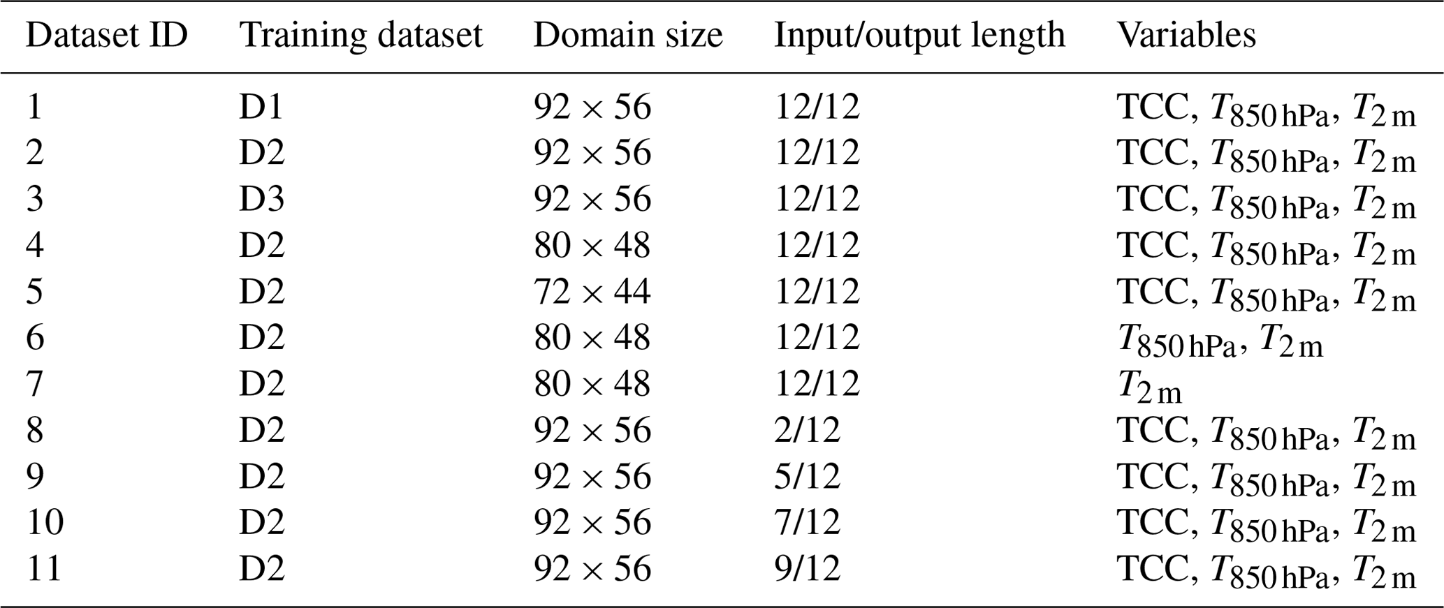
Note: D1, D2, and D3 correspond to the three datasets where the number of years in the training dataset is varied (11, 10, and 8 years, respectively) as illustrated in Fig. 2.

Table A2 Overview of the experiments in this study.

Appendix B: Evaluation metrics

In this section, we provide some mathematical details on the evaluation metrics used in this study that are the mean squared error (MSE), the anomaly correlation coefficient (ACC), the structural similarity index (SSIM), and the gradient ratio r_G.

B1 Mean squared error (MSE)

The MSE measures the squared difference between the model data and the ground truth data. Let x_ij and ${\widehat{x}}_{ij}$ constitute data on discrete grid points of the ground truth and the forecasts, respectively, where the grid consists of I and J cell centre positions in the zonal and meridional direction (or the width and height in pixels for images), respectively. With $N=I\times J$, the MSE reads

$$\begin{array}{}\text{(B1)}& \text{MSE}={\displaystyle \frac{\mathrm{1}}{N}}\sum _{i=\mathrm{1}}^I\sum _{j=\mathrm{1}}^J{\left[{\widehat{x}}_{ij}-x_{ij}\right]}^{\mathrm{2}}.\end{array}$$

B2 Anomaly correlation coefficient (ACC)

The ACC quantifies how well the spatial position of anomalies matches between the predicted and the ground truth data (i.e. the ERA5 reanalysis data in our case). The uncentred ACC is given by

$$\begin{array}{}\text{(B2)}& \begin{array}{rl}& \text{ACC}=\\ & {\displaystyle \frac{{\sum }_{i=\mathrm{1}}^I{\sum }_{j=\mathrm{1}}^J\left[{\widehat{x}}_{ij}-x_{ij}^c\right]\left[x_{ij}-x_{ij}^c\right]}{{\left\{{\sum }_{i=\mathrm{1}}^I{\sum }_{j=\mathrm{1}}^J{\left[{\widehat{x}}_{ij}-x_{ij}^c\right]}^{\mathrm{2}}{\sum }_{i=\mathrm{1}}^I{\sum }_{j=\mathrm{1}}^J{\left[x_{ij}-x_{ij}^c\right]}^{\mathrm{2}}\right\}}^{\mathrm{1}/\mathrm{2}}}}.\end{array}\end{array}$$

Here, $x_{ij}^c$ represents the climatological mean which is inferred at each grid point from the ERA5 reanalysis data between 1990 and 2019 in this study. Since the 2 m temperature involves a seasonal and a diurnal cycle, the climatology is calculated separately for each month of the year and each hour of the day, respectively.

B3 Structural similarity index (SSIM)

The SSIM constitutes a score metric typically applied in computer vision to measure the similarity between two images (Wang et al., 2004). It measures and compares the structural information between the ground truth and prediction images. The similarity is thereby quantified in terms of luminance, contrast variance, and structure. In the case of images with multiple channels (i.e. RGB images), the calculations are done separately for each channel and averaged afterwards.

• Luminance: the luminance is measured by averaging the pixels' brightness of the images. Letting μ_X and ${\mathit{\mu }}_{\widehat{X}}$ denote the averaged brightness of the pixels from the ground truth and the generated image, the respective component l of SSIM is given by

  $$\begin{array}{}\text{(B3)}& {\displaystyle }l={\displaystyle \frac{\mathrm{2}{\mathit{\mu }}_X{\mathit{\mu }}_{\widehat{X}}+C_{\mathrm{1}}}{{\mathit{\mu }}_X^{\mathrm{2}}+{\mathit{\mu }}_{\widehat{X}}^{\mathrm{2}}+C_{\mathrm{1}}}},\end{array}$$

  where C₁ is a constant to avoid divisions by 0 or very small numbers. Specifically, we choose C₁=(K₁L)², where K₁=0.01 and L is the dynamic range of input values. In the case of the average brightness of the two images matching, l=1 is obtained.

• Contrast: the contrast is measured by calculating separately the standard deviation of the pixel brightness of each image. Let σ_X and ${\mathit{\sigma }}_{\widehat{X}}$ denote the standard deviation of the ground truth and the generated image with

  $$\begin{array}{}\text{(B4)}& {\mathit{\sigma }}_X={\left[{\displaystyle \frac{\mathrm{1}}{N-\mathrm{1}}}\sum _{i=\mathrm{1}}^I\sum _{j=\mathrm{1}}^J(x_{ij}-{\mathit{\mu }}_X{)}^{\mathrm{2}}\right]}^{\mathrm{1}/\mathrm{2}}.\end{array}$$

  The contrast score component c then reads

  $$\begin{array}{}\text{(B5)}& {\displaystyle }c={\displaystyle \frac{\mathrm{2}{\mathit{\sigma }}_X{\mathit{\sigma }}_{\widehat{X}}+C_{\mathrm{2}}}{{\mathit{\sigma }}_X^{\mathrm{2}}+{\mathit{\sigma }}_{\widehat{X}}^{\mathrm{2}}+C_{\mathrm{2}}}}.\end{array}$$

  C₂ is added in analogy to C₁ but for the contrast score component. Here, C₂=(K₂L)² and K₁=0.03.

• Structure: the structure is computed with the help of the covariance in pixel space between the ground truth and the generated image and therefore measures the coherence between the two images in terms of variations around their average brightness. With ${\mathit{\sigma }}_{X\widehat{X}}$ denoting the covariance and using the standard deviations of the ground truth and generated image, that is σ_X and ${\mathit{\sigma }}_{\widehat{X}}$, the structural component s of SSIM is defined by

  $$\begin{array}{}\text{(B6)}& {\displaystyle }s={\displaystyle \frac{{\mathit{\sigma }}_{X\widehat{X}}+C_{\mathrm{3}}}{{\mathit{\sigma }}_X{\mathit{\sigma }}_{\widehat{X}}+C_{\mathrm{3}}}},\end{array}$$

  where $C_{\mathrm{3}}=C_{\mathrm{2}}/\mathrm{2}$ serves as an additional constant, as proposed in the study by Wang et al. (2004).

Finally, the SSIM is obtained by merging the different components together with the help of

$$\begin{array}{}\text{(B7)}& {\displaystyle }\text{SSIM}=l^{\mathit{\alpha }}\cdot c^{\mathit{\beta }}\cdot s^{\mathit{\gamma }}.\end{array}$$

Here, α, β, and γ are disposal (positive) parameters which control the importance of each score component. Here, we use $\mathit{\alpha }=\mathit{\beta }={\mathit{\gamma }}_c=\mathrm{1}$. In our particular translation, the luminance corresponds to a measure which compares the domain-averaged 2 m temperature between prediction and the respective ERA5 reanalysis data. Contrast is equivalent to a comparison between the global variability of T_2 m per time step, while the structure simply compares the covariance between the predicted and the ground truth 2 m temperature fields.

B4 Gradient ratio

The SSIM does not account explicitly account for local variability in the data. Indeed, the l and c components only evaluate the overall average and the variability. Only s measures how the data vary on a grid point (pixel-wise) level. To further analyse the local spatial variability, we calculate the amplitude of the horizontal 2 m temperature gradient. Sha et al. (2020) follow a similar approach in their temperature downscaling application but deploy the Laplace operator rather than the gradient operator. Besides, their operator does not account for the curvature on the sphere.

In the geographical coordinate system, the horizontal gradient of the arbitrary quantity ψ reads

$$\begin{array}{}\text{(B8)}& {\mathrm{\nabla }}_{\mathrm{h}}\mathit{\psi }={\displaystyle \frac{\mathrm{1}}{r_{\mathrm{E}}\cos \left(\mathit{\phi }\right)}}{\displaystyle \frac{\partial \mathit{\psi }}{\partial \mathit{\lambda }}}{e}_{\mathit{\lambda }}+{\displaystyle \frac{\mathrm{1}}{r_{\mathrm{E}}}}{\displaystyle \frac{\partial \mathit{\psi }}{\partial \mathit{\phi }}}{e}_{\mathit{\phi }}.\end{array}$$

Here, λ and φ denote the longitude and latitude, while r_E is the (averaged) Earth radius.

On a geographical grid, the amplitude of the continuous gradient operator ∇_h can be discretized with finite differences:

$$\begin{array}{}\text{(B9)}& \begin{array}{rl}{G}_{\mathit{\psi }}& =\left|{\mathrm{\nabla }}_{\mathrm{h}}\mathit{\psi }\right(i,j\left)\right|\\ & \simeq {\displaystyle \frac{\mathrm{1}}{r_{\mathrm{E}}}}\sqrt{\begin{array}{c}\frac{\mathrm{1}}{{\cos }^{\mathrm{2}}\left(\mathit{\phi }\right(j\left)\right)}{\left(\frac{\mathit{\psi }(i+\mathrm{1},j)-\mathit{\psi }(i-\mathrm{1},j)}{\mathrm{2}\mathrm{\Delta }\mathit{\lambda }}\right)}^{\mathrm{2}}\\ +{\left(\frac{\mathit{\psi }(i,j+\mathrm{1})-\mathit{\psi }(i,j-\mathrm{1})}{\mathrm{2}\mathrm{\Delta }\mathit{\phi }}\right)}^{\mathrm{2}}\end{array}},\end{array}\end{array}$$

where Δλ and Δφ denote the grid spacing of the underlying grid. i and j correspond to indices on the grid in the zonal and meridional direction, respectively. This yields a second-order accurate discretization on a regular grid (constant spacing in horizontal directions).

Now, let G_X and $G_{\widehat{X}}$ denote the average of the absolute horizontal gradient of our target quantity over all grid points on the domain (apart from the lateral boundaries) for the ground truth and the predicted data, respectively. The ratio

$$\begin{array}{}\text{(B10)}& r_{\mathrm{G}}={\displaystyle \frac{G_{\widehat{X}}}{G_X}}\end{array}$$

then measures the averaged local spatial variability amplitude in the predicted field compared to the reference data. For r_G=1, the amplitude of the horizontal gradient is on average the same in the prediction and in the ground truth. For r_G<1 (r_G>1), the horizontal gradient is on average underestimated (overestimated) by the model, indicating that the field is visually too blurry (too sharp) following the discussion in Sect. 3.

Appendix C: Supplementary figures

Figure C1 MSE over 9 h forecast for 2 m temperature with inter-decile bootstrap confidence intervals (shading area) using WeatherBench convolutional neural network and persistence forecasting.

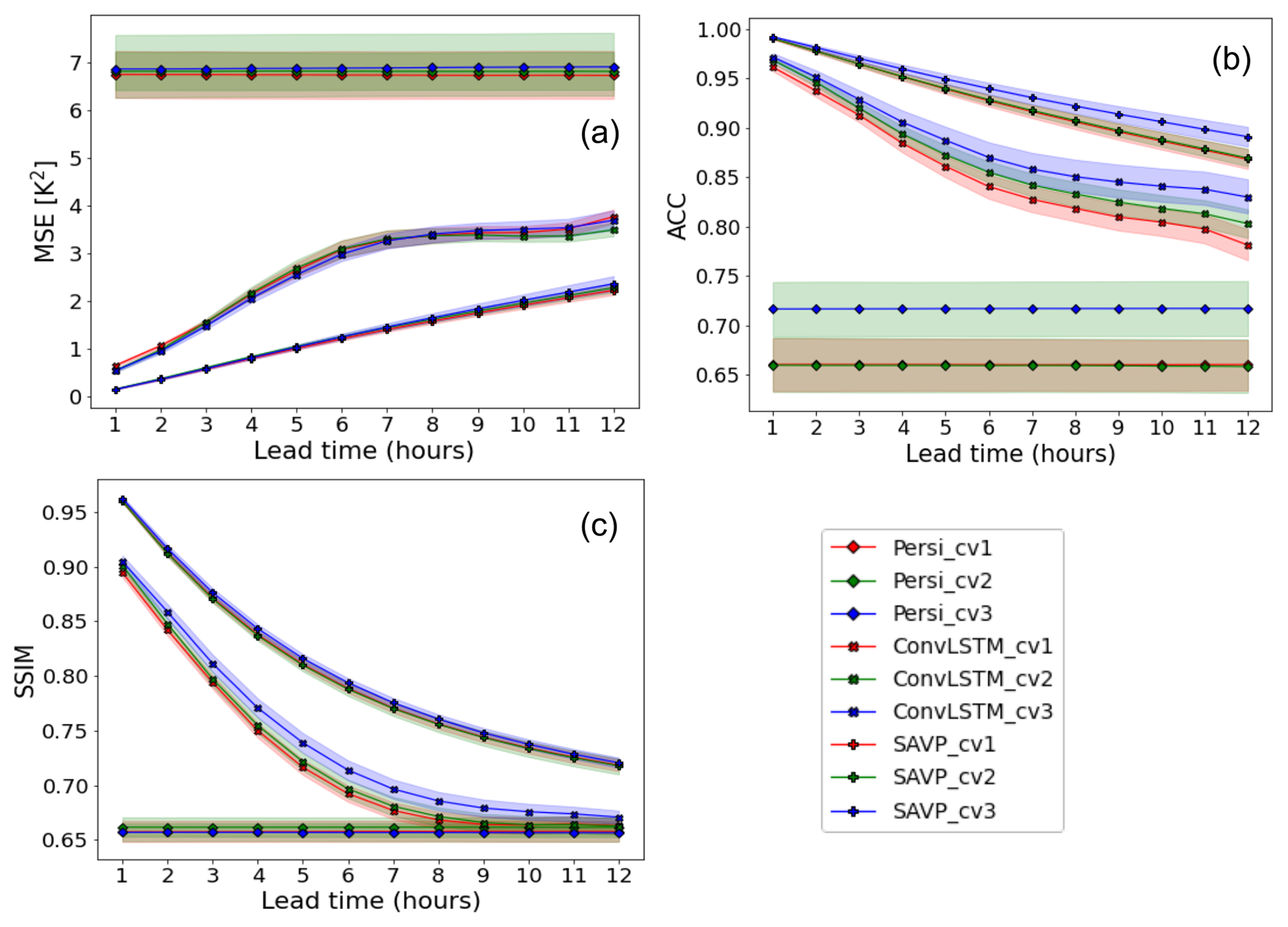
Figure C2 Averaged (a) MSE, (b) ACC, and (c) SSIM across lead time (x axis) for the SAVP, the ConvLSTM, and the persistence forecasts from Experiment 1 in Table A2. Like in Fig. 2, sampling uncertainty is estimated via block bootstrapping. However, the inter-decile confidence range is now colour shaded for the three cross-validation datasets using different models.

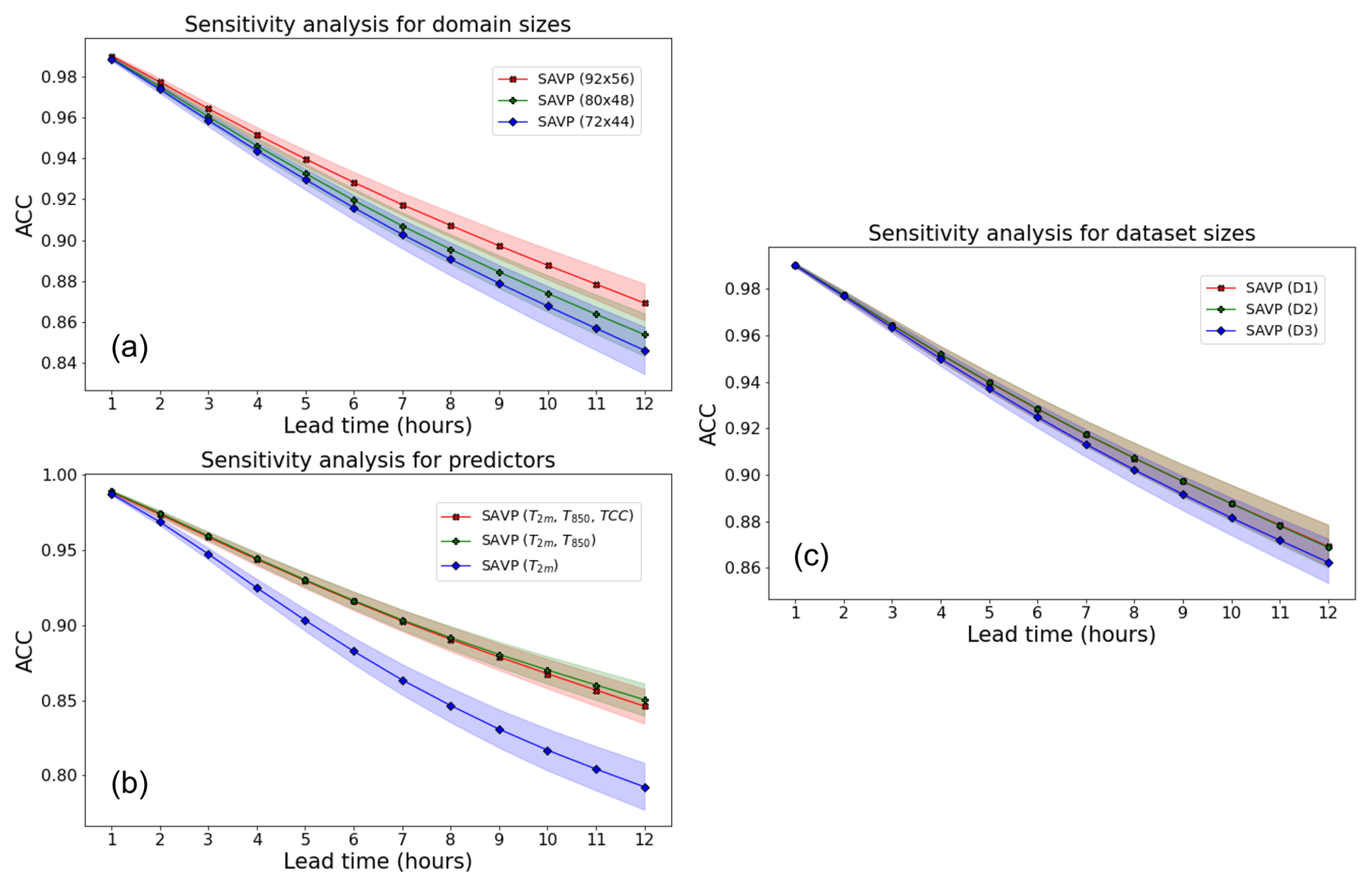
Figure C3 Averaged ACC over the forecast period for 2 m temperature with the SAVP model for different sensitivity experiments using (a) different domain sizes (red – 92 × 56; green – 80 × 48; blue – 72 × 44), (b) different predictors (red – T_2 m, T_850 hPa, and TCC; green – T_2 m, T_850 hPa; blue – T_2 m), and (c) different sizes of the training dataset (red – 11 years; green – 10 years; blue – 8 years). The inter-decile confidence range (colour shaded) is estimated via block bootstrapping.

Figure C4 Like Fig. C3 but for SSIM.

Figure C5 Like Fig. C3 but for the gradient ratio r_G.

Figure C6 Analogous to Fig. 6 but for additional lead times (1, 3, 5, 7, 9, and 11 h).